Submitted:
05 February 2026
Posted:
06 February 2026
You are already at the latest version
Abstract
Understanding the microstructure of brain tumours without invasive methods remains a major challenge in neuro-oncology. The VERDICT MRI technique provides biologically meaningful metrics, such as cellular and vascular fractions, that help distinguish tumour grades and align closely with histological findings [1,2]. Yet, traditional non-linear fitting approaches are both computationally heavy and prone to errors, which restricts their use in clinical practice. Deep learning presents a promising solution by enabling faster and more reliable diffusion analysis [3]. Still, there is limited evidence on which specific neural network designs are best suited for accurate VERDICT parameter mapping. We present the first head-to-head benchmark of eight neural network families for predicting VERDICT parameters: multilayer perceptron (MLP), residual MLP, Long short-term memory (LSTM)/Recurrent Neural Network (RNN), Transformer, 1D-Convolutional Neural Networks (CNN), variational autoencoder (VAE), Mixture of Experts (MoE), and TabNet. All models were trained and evaluated under a unified protocol with standardized preprocessing, matched optimization settings, and common metrics (coefficient of determination R2, RMSE), supplemented with bootstrap-based uncertainty and pairwise significance testing. Across targets, simple feedforward baselines performed competitively with more complex sequence and attention-based models, indicating that architectural complexity does not uniformly translate into superior accuracy for VERDICT regression on tabular features. Compared to traditional fitting, learned predictors enable fast inference and streamlined deployment, suggesting a practical path toward near-real-time VERDICT mapping. By establishing performance baselines and a reproducible evaluation protocol, this benchmark provides actionable guidance for model selection and lays the groundwork for clinically viable, learning-based microstructure imaging in neuro-oncology.
Keywords:
diffusion modeling
; microstructure
; deep learning
; brain tumor
; model fitting
1. Introduction and Background
1.1. Introduction
Quantitative assessment of tissue microstructure is fundamental to modern medical imaging, particularly in oncology, where understanding tumour composition directly influences diagnosis, treatment planning, and monitoring therapeutic response [4]. Conventional structural magnetic resonance imaging (MRI) techniques, such as T1-weighted, T2-weighted, and FLAIR sequences, are widely used in clinical practice and provide excellent anatomical detail. However, these methods lack the specificity required to characterize tissue microstructure non-invasively [1,4].
To address this limitation, diffusion MRI has become an essential tool in clinical neuroimaging and oncology. Standard approaches such as diffusion tensor imaging (DTI) and the apparent diffusion coefficient (ADC) model are already routinely employed to assess tissue integrity and detect abnormalities. While these techniques offer quantitative biomarkers related to tissue microstructure, for example, DWI (and derived ADC) is widely used across cancer types to distinguish lesion types, grade tumours, predict treatment response, and detect recurrence [5]. Complex heterogeneity of tumour tissue-despite ADC correlates inversely with cellularity, and it cannot fully capture microstructural complexity [6].
In response, advanced diffusion models have been proposed to achieve greater specificity. Among them, VERDICT (Vascular, Extracellular, and Restricted Diffusion for Cytometry in Tumours) MRI stands out as a promising technique for quantitative microstructural analysis of tumours [1]. VERDICT employs multi-compartment diffusion modelling to estimate parameters such as vascular volume fraction, extracellular-extravascular space fraction, and restricted intracellular diffusion characteristics that reflect cellular density and size. Importantly, the VERDICT model for brain tumours is more elaborate than the simplified versions often applied in body tumours, as it incorporates additional anisotropic extracellular compartments and orientation parameters. While this complexity offers richer biological interpretability, it also increases the computational burden and makes robust parameter estimation more challenging.
Despite these advantages, the computational complexity of VERDICT parameter estimation presents a barrier to clinical translation. Traditional fitting approaches rely on iterative optimization, which is computationally expensive, prone to local minima, and sensitive to noise, limiting their practicality in routine workflows [7].
The emergence of deep learning has transformed medical image analysis [8]. Neural networks can learn complex mappings from diffusion MRI signals to microstructural parameters, offering the potential for faster and more robust estimation [9]. However, the medical imaging community still lacks comprehensive benchmarking frameworks to systematically evaluate different neural network architectures for VERDICT parameter prediction.
This work addresses this gap by presenting a comprehensive benchmark suite specifically designed for evaluating deep learning approaches to VERDICT parameter prediction. Our benchmark encompasses diverse neural network architectures: from simple multilayer perceptrons to advanced Transformer and provides rigorous statistical evaluation protocols to ensure fair and meaningful comparisons. The framework is designed to support reproducible research and facilitate the identification of optimal architectures for medical parameter prediction tasks. In particular, we focus on the brain tumour VERDICT model, which is more complex than its body tumour counterparts and therefore represents a more challenging and clinically significant use case.
1.2. VERDICT MRI: Overview and Clinical Applications
Overview.
The Vascular, Extracellular and Restricted Diffusion for Cytometry in Tumours (VERDICT) model was introduced as a multi-compartment framework that explicitly accounts for distinct water pools in tumour tissue [1]. Figure 1 illustrates this concept: the MRI signal is modelled as a combination of contributions from intracellular space, the extravascular extracellular space (EES), the micro vasculature, and a free-water compartment, each corresponding to a specific microstructural component of the tumour [10,11]. By fitting this model to advanced diffusion-weighted data, one can estimate biologically meaningful parameters, including cell size, intracellular volume fraction, extracellular (stromal) volume fraction, and a pseudo-diffusion coefficient for capillary flow - thereby performing an in vivo ’cytometry’ of the tumour [2].
Panagiotaki et al. (2014) demonstrated that VERDICT-derived metrics (e.g. cell size and volume fractions) agree well with histological measurements and that the model captures tumour microstructure more accurately than standard diffusion models (ADC or IVIM) [1]. Subsequent studies have reinforced the clinical relevance of this approach: for example, Johnston et al. (2019) showed that the VERDICT-derived intracellular volume fraction is highly repeatable and better differentiates aggressive tumors from benign tissue than ADC measurements [12]. In brain tumours, VERDICT MRI has similarly proven valuable; Zaccagna et al. reported that VERDICT parameters in gliomas correlate with histopathological indices of cellularity and vascularity, revealing differences between high- and low-grade tumours that conventional diffusion MRI could not discern [2]. These findings underscore the biological rationale and clinical potential of the VERDICT model in brain tumour imaging, as it disentangles microstructural features into interpretable compartments and provides compartment-specific insights beyond the reach of traditional diffusion MRI.
Clinical relevance.
VERDICT parameters have direct biological interpretations. Elevated correlates with high cellularity and tumour grade; reflects angiogenesis and can inform response to anti-angiogenic therapies; extracellular metrics (, , , , ) capture tissue organization and edema/infiltration patterns [2,12,13,14]. In prostate cancer, VERDICT parametric maps—particularly —outperform conventional ADC for lesion detection and characterization, with reported AUC improvements of ∼0.15–0.20 [12,13]. Applications to bone metastases and brain tumours further support reproducibility and utility across diseases [2,14,15]. In brain tumours, high-grade lesions (e.g., glioblastomas, metastases) often exhibit elevated (∼0.2–0.4), while low-grade gliomas show lower values (∼0.1). Peritumoral vasogenic edema around metastases typically presents higher and lower anisotropy than the more anisotropic, infiltrative margins of gliomas [14].
Acquisition and practical considerations.
1.3. Computational Challenges in VERDICT Parameter Estimation
Classical estimation (non-linear least squares or maximum likelihood) must navigate a high-dimensional, non convex landscape under biophysical constraints, leading to:
- 1.
- Computational complexity: expensive iterative solvers with costly forward models/Jacobians [16].
- 2.
- 3.
- Local minima and initialization sensitivity: non convexity yields inconsistent fits across starting points.
- 4.
- Noise sensitivity: high-b acquisitions are SNR-limited, degrading stability and biasing estimates [7].
- 5.
- Clinical feasibility: per-slice runtimes on the order of minutes hinder real-time mapping and workflow integration.
These limitations motivate learning-based surrogates that amortize inference by replacing iterative optimization with a single forward pass.
1.4. Deep Learning for Medical Parameter Prediction
Deep neural networks approximate the inverse mapping from diffusion signals to microstructural parameters, offering: (i) computational efficiency via fast feed-forward predictions; (ii) noise robustness learned through augmentation and loss design; (iii) capacity for complex non-linear relationships; and (iv) end-to-end learning from raw or minimally processed inputs [3,9,17]. Early q-space deep learning showed accelerated microstructure mapping from undersampled data [9]; subsequent work matched or exceeded conventional fitting while providing substantial speed-ups and improved robustness under low-SNR or suboptimal protocols [3]. However, systematic, architecture-level evaluations and standardized protocols tailored to VERDICT remain limited.
1.5. Research Gap and Motivation
The literature reveals: (1) limited architectural exploration beyond single-model studies; (2) inconsistent evaluation protocols (datasets, metrics, validation); (3) lack of standardized benchmarks for reproducible comparison; (4) insufficient statistical rigour (significance testing, confidence intervals); and (5) limited clinical context (interpretability, uncertainty, runtime) [3,9,12,13]. These gaps motivate a comprehensive, reproducible benchmark for deep learning approaches to VERDICT parameter prediction.
1.6. Thesis Contributions and Objectives
This thesis introduces the first comprehensive benchmark of deep learning architectures for VERDICT parameter estimation:
- Comprehensive architecture evaluation: feedforward, convolutional, recurrent, Transformer-based, and advanced (Variational Auto-encoder, Mixture of Experts) models under a unified pipeline.
- Standardized evaluation: rigorous protocols with bootstrap confidence intervals and significance testing for fair, meaningful comparisons.
- Reproducible platform: open-source implementations, configurations, and scripts for community use and extension.
2. Data
2.1. Overview and Rationale
We generate a large-scale synthetic dataset of diffusion-weighted MR signals to train and validate signal-model–based inference for VERDICT applications in brain tumours. Unlike earlier approaches that relied on reference labels estimated from “real” data (e.g., parameter maps obtained by non-linear least squares (NLLS) fitting) [1,2], we follow the synthetic-signal paradigm, in which training/validation signals are simulated from a forward biophysical model and paired with their ground-truth microstructural parameters.1 For the fixed considered acquisition scheme (set of M diffusion encodings with b-values and gradient/b-tensor orientations ), we simulate parameter combinations where . These eight degrees of freedom correspond to the free parameters in the VERDICT model variant used for brain tumours. For completeness, the full parameterization includes the intracellular, extracellular, and vascular fractions , the intra-cellular diffusivity , the extracellular axial and radial diffusivities , the cell radius R, and the orientation angles . The vascular pseudo-diffusivity is also part of the model but fixed to a constant value in this implementation. Thus, although 10 quantities appear in the parameterization, only eight are free, since (i) is derived by , and (ii) is fixed.
Acquisition Scheme [14]
MRI was performed preoperatively with a 3.0T Ingenia CX scanner (Philips Healthcare, Best, The Netherlands) at the Neuroradiology Unit and CERMAC, IRCCS Ospedale San Raffaele (Milan, Italy) [14]. Conventional MRI including 3D-FLAIR images (TE/TI/TR = 285/2500/9000 ms, isotropic resolution 0.7 mm) and post-contrast 3D T1-weighted images (TE/TR = 5.27/11.12 ms, flip angle 8 degrees, isotropic resolution 0.5 mm) were acquired [14].
dMRI scans were acquired using the parameters summarised in Table 1 and with an isotropic voxel size of 2 mm. Nineteen of the patients also had perfusion MRI, including dynamic contrast-enhanced (DCE) 3D spoiled gradient echo sequences (TE/TR = 1.8/3.9 ms, flip angle 15 degrees, in-plane resolution 2 x 2 , slice thickness 2.5 mm, 70 repetitions) and dynamic susceptibility contrast (DSC) fast field echo EPI sequences (TE/TR = 31/1500 ms, flip angle 75 degrees, in-plane resolution 2 x 2 , slice thickness 5 mm, 80 repetitions). [14]
Model parameterization and constraints.
To maintain biophysical plausibility and improve numerical conditioning, VERDICT parameters are reparameterized with smooth, bounded transforms that facilitate gradient-based optimization [1,7,16]. The extracellular anisotropic compartment is commonly modelled as an axially symmetric Gaussian (“Zeppelin”) for brain tumours (though not typically in most body applications of VERDICT), whose principal axis is defined by spherical angles [19].
- Intracellular volume fraction (): with , enforcing ; a noninvasive surrogate for cellularity [1].
- Vascular volume fraction (): , indexing the fraction of signal arising from the vascular space.
- Intracellular diffusivity (): , reflecting apparent intracellular diffusion.
- Cell radius (R): , sensitive to cell size distribution/morphology [1].
- Extracellular axial diffusivity (): along the Zeppelin axis.
- Extracellular radial diffusivity (): in the deep learning implementation, this is obtained indirectly by predicting a multiplier , such that . This constrains by construction.
- Orientation angles: and define the Zeppelin axis [19].
- Vascular pseudo-diffusivity (): fixed to in this implementation (as in [14]), but still a parameter of the vascular compartment.
This construction (i) guarantees non-negative fractions that sum to unity, (ii) respects diffusivity ordering in the anisotropic compartment, (iii) explicitly accounts for vascular pseudo-diffusion as a fixed parameter, and (iv) yields smooth objectives that are better conditioned for optimization [1,7,16].
2.2. Acquisition Model and Units
For single diffusion encoding (Stejskal–Tanner PGSE), the diffusion-weighting is quantified by
where is the gyromagnetic ratio, g is gradient amplitude, and are the gradient pulse duration and separation, respectively [20]. In all simulations, model diffusivities are expressed in and b-values in ; measured b-values in are converted by .
2.3. VERDICT Signal Model
The voxel signal is a convex mixture of three canonical compartments (restricted intra-cellular spheres, hindered extra-cellular/extravascular “zeppelin”, and vascular “astrosticks”):
with , . Here R is the cell-radius, the intra-cellular diffusivity, the parallel/perpendicular diffusivities of the zeppelin, its principal axis, and the vascular pseudo-diffusivity. is the non-diffusion-weighted signal.
Restricted spheres (intra-cellular).
is the normalized PGSE signal for impermeable spheres of radius R and diffusivity at finite . We evaluate it numerically using the standard eigenmode-series solution employed in VERDICT modelling (as in [1]), which accounts for finite gradient timing.
Hindered zeppelin (extra-cellular/extravascular).
Assuming a Gaussian anisotropic compartment with axis and diffusion tensor , the single-encoding signal under a unit direction is
i.e., the standard anisotropic Gaussian attenuation [21].
Astrosticks (vascular).
For a stick compartment with diffusion only along its axis and an isotropic orientation distribution under linear tensor encoding, we are assuming that the sticks are physically oriented in all directions but we keep the directional acquisitions separate. The attenuation admits the closed form
where is the error function [22]. Following prior VERDICT work in tumours, we fix unless stated otherwise [14].
2.4. Signal Synthesis for One Acquisition Scheme
For a particular acquisition which is specific for our simulation , the continuous parameters are sampled within the ranges shown in Table 2 and one synthetic example is generated as follows:
- 1.
- Sample a parameter tuple .
- 2.
Repeating the above for i.i.d. draws of yields a matrix of synthetic signals with paired ground truth parameters .
2.5. Context Within VERDICT Literature
The compartment choice and constraints in (2) follow the VERDICT framework introduced for tumour microstructure imaging [1] and subsequently adapted to brain tumours, where fixing the vascular pseudo-diffusivity can improve robustness [14]. Our use of synthetic signals directly from the forward model avoids propagating bias from noisy NLLS estimates (e.g., as used in earlier real-data–based training) and aligns with the synthetic-signal training concept in diffusion MRI [18]. For completeness, the zeppelin Gaussian attenuation (3) is consistent with the DTI formulation [21], and the powder-averaged stick closed form (4) under linear tensor encoding is standard in axisymmetric b-tensor analyses [22].
3. Models and Methodology
3.1. Experimental Framework
We evaluate eight neural network architectures for VERDICT MRI parameter prediction, spanning from feedforward networks to attention-based models. Implementations use PyTorch [23]. Each sample is a 153-dimensional feature vector which is number of acquired volumes in the acquisition scheme that we are considering; the networks predict eight output parameters (p1 to p8) which are used to calculate the actual eight VERDICT microstructural parameters: fractional intracellular volume , fractional extracellular volume , intracellular diffusivity , restriction radius R, parallel diffusivity , transverse diffusivity , and angular parameters . These targets originate from the VERDICT biophysical framework for tumour microstructure characterization [1].
3.2. Benchmark Neural Network Architectures
3.2.1. Multi-Layer Perceptron (MLP)
A baseline fully connected MLP with three hidden layers (150 units each) and ReLU activations serves as our tabular regression benchmark [17].
The MLP regressor is a feedforward network that maps a -dimensional feature vector to target parameters via a stack of fully connected layers and point-wise nonlinearities [17]. Let the hidden-layer widths be with H hidden layers. The network computes
where is a configurable activation (e.g., ReLU/GELU), , and . The output layer is purely linear to preserve regression fidelity.
Implementation.
There is a clear pattern to the implementation:
- Construct a list of layer widths .
- For each hidden transition , append Linear(,) and the chosen activation .
- Append the final Linear(,) without activation.
In PyTorch, this corresponds to a nn.Sequential of repeated Linear + activation blocks, terminating with a linear head:
Capacity and complexity.
The total number of trainable parameters is
and the per-forward computational cost scales as . Model capacity is controlled by H and the widths ; deeper/wider settings increase expressivity at the expense of parameters and compute [17].
Instantiation in our benchmark.
Unless stated otherwise, we use (feature dimension), (VERDICT parameters), with , and . The model is trained with mean-squared error loss under the standardized training protocol described in Section 3.3, with regularization (weight decay) and early stopping to mitigate overfitting. No skip connections, batch normalization, or dropout are used in this baseline, making it a strong yet transparent reference for tabular regression.
3.2.2. ResNet
Motivation.
As depth increases, deep feedforward networks may experience degradation and vanishing gradients. Residual learning mitigates these issues by learning residual mappings with identity skip connections, which preserve gradient flow and ease optimization [17,24]. We adapt this idea to tabular regression by inserting residual blocks into an MLP backbone.
Architecture.
Let and denote input and output dimensions, and let the hidden width be d (kept constant across residual blocks). The network consists of:
- 1.
- An input stem ,
- 2.
- Bresidual blocks with identity skip connections,
- 3.
- A linear head .
Each residual block applies two affine layers with a pointwise nonlinearity after the first, and a final nonlinearity after the skip addition (post-activation form):
Here is a configurable activation (e.g., ReLU, GELU). The identity skip requires matching input/output dimensions of the block (i.e., ).
Implementation details.
The implementation follows:
- Stem: Linear(, d) followed by .
- Residual stack: B blocks, each with Linear(d, d)→→Linear(d, d), then skip-add and .
- Head: Linear(d, ) without activation.
In code, a ResidualBlock encapsulates the two affine layers and the skip connection; a ModuleList stacks B such blocks. The provided implementation constructs blocks using the entries of hidden_dims. In practice, to satisfy the identity skip without projections, all block widths must be equal (i.e., hidden_dims contains a repeated width). If varying widths are desired, one should insert either (i) transition layers between blocks or (ii) a projection skip (e.g., a Linear(, ) on the identity path) as in [24].
Capacity and compute.
With constant width d and B blocks, the parameter count is
The forward pass has cost , with negligible overhead for the elementwise skip-add.
Training considerations.
Residual connections generally improve optimization stability and allow deeper models without suffering the degradation observed in plain MLPs [24]. We use a linear output (no activation) to preserve regression fidelity, and the same loss, regularization, and scheduler as in Section 3.3. When depth increases, consider weight decay and (optionally) dropout/batch normalization for regularization; however, our baseline omits them to isolate the effect of residual learning.
Instantiation in our benchmark.
Unless noted, we set , , choose a constant hidden width , use residual blocks, and . This yields a transparent, high-capacity baseline that typically trains faster and more reliably than a depth-matched plain MLP.
3.2.3. RNN-Based Regressor
Motivation.
Recurrent architectures model ordered dependencies and long-range interactions by maintaining a latent state across time steps. Although our inputs are flat feature vectors, reshaping them into short sequences allows an RNN to learn structured relationships that plain MLPs may miss. We instantiate vanilla RNN, LSTM, or GRU cells, which differ in gating mechanisms and memory capacity [17,25,26].
Architecture.
Given an input , we select a sequence length L (“seq_len”) and set the per-step feature size so that is reshaped to a matrix (batch dimension suppressed). If is not divisible by L, a linear projection is applied to obtain a compatible tensor with step size equal to the hidden width H (“hidden_dim”). Concretely,
An N-layer RNN (RNN/LSTM/GRU) with hidden width H processes the sequence to produce hidden states :
where denotes the chosen recurrent cell (for LSTM/GRU, includes gates as in [25,26]). We use the last hidden state as a sequence summary, apply a pointwise activation , and project to the target dimension:
Dropout is applied between recurrent layers when .
Implementation details.
The implementation (PyTorch) infers a “reasonable” L by selecting a divisor of that is not too small (preferably ) to balance step length and per-step dimensionality; otherwise, it uses a learned input projection to a compatible size. We set batch_first=True so tensors are . The forward pass performs:
- 1.
- (Optional) linear projection if ,
- 2.
- reshape to ,
- 3.
- recurrent stack (RNN/LSTM/GRU, N layers, optional dropout),
- 4.
- last-timestep pooling, activation, and a final linear layer.
Example. With , the divisor heuristic picks and (no projection). The model thus learns temporal-style dependencies over 9 steps of 17 features each.
Capacity and complexity.
Per recurrent layer, the parameter count is
plus (if used) the input projection and the output head . The time complexity scales as per sample.
Training considerations.
We apply a linear output (no activation) for regression fidelity and use the standardized training protocol of Section 3.3. For stability with deep stacks or long L, gradient clipping and careful learning-rate scheduling are recommended [17]. While last-timestep pooling is simple and effective, alternatives (mean/attention pooling) can be substituted if earlier steps carry salient information.
Instantiation in our benchmark.
Unless otherwise specified, we use rnn_type=LSTM, , , dropout (between layers), and the heuristic L (e.g., for ). The activation after the last hidden state is ReLU. This configuration offers a strong sequential baseline while keeping compute moderate.
3.2.4. Transformer Regressor
Motivation.
Self-attention models capture global, content-dependent interactions without recurrence or convolution, making them attractive for modeling complex feature dependencies in tabular diffusion-derived inputs [27]. We employ a Transformer encoder-only stack as a flexible regressor with residual connections, layer normalization, and position-wise feed-forward sublayers.
Architecture.
Let denote the input feature vector and the embedding width. The model comprises:
- 1.
- Embedding (tokenization): a linear projection We treat the entire feature vector as a single token (sequence length ), so the encoder processes a tensor (batch dimension suppressed).
- 2.
- Encoder stack: N identical layers, each with (i) multi-head self-attention (MHSA) and (ii) a position-wise feed-forward network (FFN), both wrapped with residual connections and layer normalization:where with hidden width and activation (ReLU or GELU).
- 3.
- Pooling and head: mean pooling over the (single) token and a linear regressor:
With , self-attention reduces to a learned self-gating on the single token; the stack behaves like a deep residual bottleneck MLP with MHSA/FFN structure, while retaining the benefits of normalization, residuals, and flexible depth [27].
Implementation details.
We use nn.TransformerEncoderLayer with arguments d_model, nhead, dim_feedforward, dropout, and activation (ReLU/GELU), and stack N layers via nn.TransformerEncoder. Inputs are projected by Linear(, ), reshaped to (batch_first=True), passed through the encoder, mean-pooled across the (single) token, and mapped to by a final linear layer. No positional encodings are used since .
Complexity.
For a general sequence length L, a single encoder layer costs
In our design with , the attention term becomes negligible, and the cost is dominated by the FFN: per layer.
Instantiation in our benchmark.
Unless stated otherwise, we set , nhead, encoder layers, , dropout , activation , and a linear output head. The model is trained with mean-squared error under the standardized protocol of Section 3.3.
Notes on sequence construction.
While offers a strong, stable baseline, attention mechanisms are most beneficial when . In practice, one can increase L by chunking features into tokens or learning a feature tokenizer, and optionally adding positional encodings, to allow MHSA to model cross-token interactions [27].
3.2.5. Advanced 1D CNN Regressor with Multi-Scale Attention
Motivation.
Convolutional networks capture local patterns with shared filters and are effective for 1D signals or feature sequences [28]. We augment a 1D CNN backbone with (i) multi-scale convolutions to detect patterns at different receptive fields [29], (ii) channel and spatial attention to emphasize informative responses [30,31], and (iii) residual connections to improve optimization and enable depth [24]. Global pooling and a compact MLP head yield length-agnostic regression.
Architecture.
Given an input vector , we reshape to and apply:
- 1.
- Embedding stem: , where is the chosen activation.
- 2.
- Feature stages (): each stage stacks a MultiScaleConvBlock and (optionally) a ResidualBlock, followed (except the last stage) by adaptive downsampling:where and (doubling across stages).
- 3.
- Global aggregation: global average and max pooling on the final feature map :
- 4.
- Head: a two-layer MLP with batch normalization, activation, and dropout, followed by a linear regressor to :
Attention modules.
Channel attention (CA). For a feature map , we compute global descriptors by average and max pooling, pass them through a bottleneck MLP with reduction ratio r (default ), sum the outputs, and gate channels with a sigmoid [30,31]:
Spatial attention (SA). We pool across channels (avg and max), concatenate the two 1D maps, and apply a convolution (here ) plus sigmoid to gate salient temporal locations [30]:
Implementation notes.
The PyTorch implementation:
(i) embeds to by a stem;
(ii) repeats MultiScaleConvBlock (four kernels: 3/5/7/11) with BN+activation and CBAM-style attention, optionally followed by a ResidualBlock (Conv-BN--Conv-BN-skip-); (iii) uses AdaptiveAvgPool1d to halve length per stage (except the last); (iv) aggregates with global avg/max pooling and concatenation; and (v) predicts via an MLP head with BN, dropout, and a final linear layer. Weight initialization uses Kaiming (He) init for conv layers [32] and unit-gamma/zero-beta for batch norm [33], with small normal init for linear layers. The design is length-agnostic due to adaptive pooling and global pooling [34].
Complexity.
Per stage, the multi-scale branch cost is , followed by two residual convolutions . Downsampling reduces , so later stages are cheaper. The head is dominated by its first linear layer of size .
Instantiation in our benchmark.
We set , , base filters , number of stages , activation , dropout , and use_residual. This yields a strong CNN baseline that combines multi-scale pattern extraction, attention-driven emphasis, and residual learning while keeping parameter count and runtime moderate.
Training.
We use a linear output head for regression fidelity and the standardized training protocol in Section 3.3 (MSE objective, weight decay, cosine schedule). Optional regularizers (e.g., stronger dropout) can be enabled if overfitting is observed.
3.2.6. Variational Autoencoder (VAE) Regressor
Motivation.
Variational autoencoders learn a low-dimensional latent representation by maximizing a tractable evidence lower bound (ELBO) under a generative model with a simple prior [35]. For VERDICT regression, a VAE can act as a regularized feature extractor: the latent code is shaped by a Kullback-Leibler (KL) penalty toward a prior, which encourages smooth, information-efficient embeddings and can improve robustness to noise. We augment the latent space with a supervised head to predict VERDICT parameters directly, while retaining an autoencoding decoder for reconstruction-based regularization.
Architecture.
Let denote the input features and the target parameters. The encoder is an MLP producing the mean and (log) variance of a diagonal Gaussian posterior,
with standard normal prior . We draw a latent sample via the reparameterization trick,
pass it to a decoder that reconstructs , and to a regression head that predicts . Concretely, our implementation uses:
- Encoder: MLP with hidden widths specified by hidden_dims, activation (e.g., ReLU/GELU), and optional dropout; linear heads produce and of size .
- Decoder: mirrored MLP mapping back to .
- Regressor: small MLP mapping to .
Objective.
We combine a supervised regression loss with the VAE reconstruction and KL terms. Using mean-squared error (MSE) for both regression and reconstruction (Gaussian likelihood) [17,36], the per-batch objective is
with weighting coefficients . For a diagonal Gaussian posterior, the KL term admits the closed form
The hyperparameter controls the strength of latent regularization (cf. -VAE) and trades off reconstruction fidelity against disentanglement/capacity. The coefficient scales the auxiliary reconstruction term, which encourages the latent to retain signal structure helpful for prediction.
Implementation details.
The encoder/decoder are constructed from Linear+ (+ optional dropout) layers; the regression head is a lightweight MLP. During forward, we return so that (27) can be computed in the training loop. In code, the KL term is implemented as
We use a linear output (no activation) for to preserve regression fidelity.
Training considerations.
We adopt the standardized protocol of Section 3.3 (optimizer, schedule, early stopping). Practical tips include: (i) start with and tune upward if latent collapse is not observed; (ii) adjust to balance reconstruction and supervised terms (too large may overemphasize autoencoding); (iii) enable dropout in deeper encoders to reduce overfitting. At inference, only the regressor is needed; the decoder can be retained for qualitative checks (e.g., input consistency) or uncertainty probing via latent sampling.
Instantiation in our benchmark.
Unless stated otherwise, we set , , latent size , hidden_dims , , dropout , and . This configuration provides a compact latent bottleneck that regularizes learning while delivering competitive regression accuracy.
3.2.7. Mixture of Experts (MoE) Regressor
Motivation.
Heterogeneous input–output relations can be modeled effectively by partitioning the input space and assigning specialized predictors to different regions. Mixture-of-Experts (MoE) architectures implement this idea by combining multiple experts via a learned, input-dependent gating function [37]. Sparse/top-k gating further improves efficiency by activating only a few experts per input while retaining competitive accuracy [38].
Architecture.
Given , we first apply input normalization and a residual linear projection:
where is a pointwise nonlinearity (e.g., ReLU). The model comprises E experts (independent MLPs) and a gating network that outputs mixture weights. For dense MoE,
For sparse MoE with top-K selection, let be the indices of the K largest logits. We renormalize the selected weights and combine only those experts:
To promote load balancing during training, small Gaussian noise can be added to the gating logits before the softmax (disabled at evaluation). A final LayerNorm calibrates the output: .
Implementation details.
- Experts: each expert is a feedforward MLP with hidden widths expert_hidden_dims and dropout between hidden layers; the last layer is linear to preserve regression fidelity.
- Gating network: a shallow MLP (input →hidden→hidden/2→ E) with dropout outputs unnormalized logits; softmax yields mixture weights.
- Pre/post processing: input LayerNorm and a residual linear projection improve conditioning; output LayerNorm stabilizes training across experts.
- Sparsity: if top_k < num_experts, only the selected experts are evaluated/combined; otherwise, all experts contribute.
Capacity and compute.
Let E be the number of experts, each with parameter count , and for the gate. Dense MoE costs expert evaluations per example; sparse top-K reduces this to , with negligible overhead for selection and renormalization [38]. The representation capacity grows roughly linearly with E, while computation scales with K.
Training considerations.
We use mean-squared error for the regression objective under the standardized protocol (optimizer, scheduler, early stopping). Practical tips include: (i) enable small gating noise during training for better expert utilization; (ii) tune E and K jointly (e.g., and ); (iii) monitor mixture entropy and per-expert load to avoid collapse where a few experts dominate.
Instantiation in our benchmark.
Unless stated otherwise, we set , , experts with [128, 64] hidden widths, gating hidden size 64, activation , dropout , gating noise std , and top_k (dense) or 2 (sparse). We report both predictions and gating weights for interpretability and analysis of specialization.
3.2.8. TabNet Regressor with Ghost Batch Normalization
Motivation.
TabNet performs sequential feature selection with learned attention masks, enabling high accuracy on tabular data while providing intrinsic interpretability [39]. Each decision step selects a (sparse) subset of features to process via gated nonlinear units (GLUs), and the model aggregates step-wise decisions into the final prediction. To stabilize training on minibatches, we employ Ghost Batch Normalization (GBN), which applies batch norm over small virtual chunks of a larger batch [40].
Building blocks.
Ghost BatchNorm (GBN). Given a batch and a virtual size , GBN splits X along the batch dimension into chunks and applies BatchNorm1d independently to each, then concatenates the results. This preserves the regularizing effect of small-batch statistics while allowing large-batch training.
Gated Linear Unit (GLU). A GLU maps to
where are affine transforms and is the logistic sigmoid. In our implementation, a single linear layer produces followed by GBN and channel-wise split.
Feature Transformer (FT). Each FT block applies GLU layers shared across steps, followed by step-specific GLUs with residual scaling:
promoting stable deep gating while allowing step-specific specialization.
Attentive Transformer (AT) Given the step’s attention features and a prior mask that discourages repeated reuse, the AT produces a normalized mask over raw inputs:
where is a learned linear map. (TabNet originally employs sparsemax; we use softmax here for simplicity [39].)
End-to-end step-wise computation.
Let be the standardized input after an initial GBN. For decision steps :
Finally, a linear head maps the accumulated decision vector to the regression targets:
Interpretability.
The masks provide step-wise feature attributions. We expose both per-sample masks and their sum across steps as a feature-importance score; dataset-level importance is computed by averaging across samples.
Implementation details.
Our PyTorch module follows [39]: (1) an input GBN; (2) T pairs of (FeatureTransformer, AttentiveTransformer); (3) decision accumulation with ReLU on the decision part; (4) a final linear mapping. The AttentiveTransformer projects attention features ( ) back to the input dimensionality D and multiplies by the current prior before normalization. Virtual batch size for GBN defaults to 128, and the prior update uses .
Instantiation in our benchmark.
Unless stated otherwise, we use , , , , , , GBN virtual batch size , and momentum . This mirrors standard TabNet settings for tabular regression while preserving interpretability through attention masks.
3.3. Training Methodology
3.3.1. Hyperparameter Configuration
All models trained up to 400 epochs on a single NVIDIA GeForce RTX 4080 Laptop GPU with batch size 16, initial learning rate , and weight decay . We used an 80/20 train–validation split and early stopping (patience 40 epochs) on validation loss [41]. Random seeds were fixed for reproducibility.
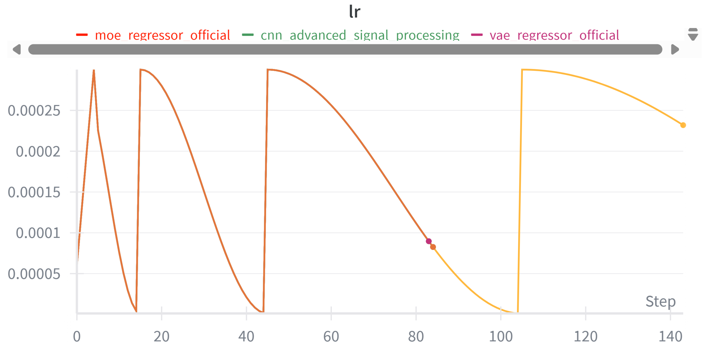
3.3.2. Learning Rate Scheduling
Cosine annealing with warm restarts (SGDR) [42] was used across models with , , , and 5 warmup epochs to improve convergence.
Figure 2.
Learning rate variation showing warmup and cosine annealing with scheduled restarts.
3.3.3. Data Preprocessing
Inputs were standardized (z-scored) using training-set statistics; scalers were saved and reused for validation/test. Targets were normalized to stabilize optimization across disparate ranges [36].
3.4. Evaluation Metrics
We evaluate model performance using the coefficient of determination (), root mean squared error (RMSE), and mean absolute error (MAE). Metrics are reported both in aggregate and for each parameter individually. Statistical significance is assessed using bootstrap confidence intervals and pairwise comparisons over resampled test sets [43].
Formally, given ground-truth values and predictions , the metrics are defined as:
where denotes the sample mean of the ground-truth values.
3.5. Implementation Details
4. Results and Analysis
This section presents aggregate and per-parameter results for all benchmark architectures: covering uncertainty, error profiles, learning dynamics, and accuracy-complexity trade-offs-and includes tumour-region parameter prediction on real patients.
4.1. Model Performance
Figure 3 summarizes test performance (primary metrics: , RMSE, MAE) across models. Bars are ordered consistently, enabling visual comparison of accuracy and error magnitude. We observe tight clustering among the top models, while several higher-capacity variants do not uniformly translate to lower error-consistent with our findings that architectural complexity alone is not a guaranteed predictor of performance on this tabular VERDICT task.
4.1.1. Uncertainty via Bootstrap Confidence Intervals
To quantify uncertainty, we compute 95% confidence intervals (CIs) for each metric using non-parametric bootstrap. Figure 4 shows CIs for , RMSE, and MAE, highlighting the best model per metric (gold). Overlapping CIs indicate statistically indistinguishable performance among the top contenders, whereas non-overlapping intervals suggest reliable differences.
4.1.2. Correlation Structure Across Parameters
Figure 5 reports the Pearson correlation between predictions and ground truth for each target (columns) and model (rows). Two patterns stand out.
(i) Easy parameters. Parameters fic and fee show consistently high agreement across all models ( to 0.97). Parameters R, Dpar, Dtra, theta, phi are moderate ( to 0.71), with small gaps between models.
(ii) Hard parameter. Parameters Dic is clearly more difficult: most models achieve only -0.60. The moe_regressor is particularly weak on these ( on Dic and slightly negative on Dpar), suggesting unstable expert specialization or a mismatch between features and these outputs. This finding is also consistent with the clinical insight that the intracellular diffusivity is known to be unstable.
Overall, the heatmap highlights heterogeneous task difficulty: global metrics mask per-target weaknesses. Practical next steps include re-weighting the multi-task loss (e.g., uncertainty weighting), adding parameter-specific heads, and targeted feature engineering/augmentation for Parameter Dic.
Moreover, it is important to acknowledge that parameters associated with compartments that occupy only a small fraction of the voxels are inherently difficult to estimate, as their influence on the overall signal is limited. At the same time, when the fraction of such compartments is negligible, these parameters are of limited practical relevance. For example, if the intracellular fraction () constitutes only 1% of the voxels, the precise estimates of cell size or intracellular diffusivity become inconsequential. In experimental data, this issue commonly arises when the intracellular fraction () is low (or the vascular fraction when vascular diffusivity is unconstrained; in the present case, the vascular compartment has no free parameter). In simulations, low extracellular fractions () may also occur. To mitigate such issues, it is common practice to threshold or weight parameter estimates according to the corresponding compartment fraction in the future implementation.
4.1.3. Error Behavior and Residual Diagnostics
Figure 6 shows residual histograms () for all models. Distributions are approximately symmetric and centered near zero-means lie within -indicating little systematic bias. The key difference is spread: moe_regressor and residual_mlp exhibit the smallest standard deviations (), followed closely by CNN/MLP/Transformer (). VAE is slightly wider (), while TabNet and RNN are widest ( and ), matching their higher RMSE/MAE. Tails are light to moderate with few outliers beyond . Overall, the models appear well-calibrated on average; further gains are more likely from reducing variance than correcting bias.
4.1.4. Learning Dynamics
Figure 7 and Figure 8 show the training and validation losses over epochs. The training loss drops rapidly at the start and then decreases more gradually, indicating stable optimization. The validation loss follows the same trend and plateaus after the initial descent, with only small stochastic fluctuations. The gap between the curves remains modest, suggesting limited overfitting.
We employ early stopping based on the best validation loss: once no improvement is observed for a fixed patience window, training halts and the checkpoint at the minimum validation loss is retained. In practice, this yields a model near the knee of the learning curve-avoiding unnecessary epochs while preserving generalization.
4.1.5. Complexity and Performance Trade-Off
Figure 9 relates model size (x–axis; estimated parameter count) to three metrics (y–axis). Overall, the relationship between complexity and performance is weak.
R2.
There is only a slight upward trend with size, and it is not decisive: the compact residual_mlp (∼500 params) attains the highest , while the much larger transformer (∼2k params) is not clearly better than smaller CNN/MLP variants.
RMSE and MAE.
Trend lines slope mildly downward, suggesting only marginal error reductions with more parameters. In practice, several small models (residual_mlp, moe_regressor, cnn, mlp) already achieve the lowest RMSE/MAE values, whereas rnn, tabnet_regressor, and vae_regressor underperform despite comparable or larger sizes.
Takeaway.
Increasing model size alone does not guarantee better outcomes. Compact architectures with appropriate inductive biases deliver competitive—often best—accuracy, offering a superior accuracy/complexity trade-off.
4.2. Rankings and Summary Table
We compares eight architectures on five criteria: , RMSE, MAE, MSE, and the mean Pearson correlation with the ground truth. Overall, the top four models are tightly clustered (differences in the third decimal place), while TabNet, VAE, and RNN trail across most metrics.
4.2.1. Overall Ranking Methodology
The overall ranking system provides a comprehensive assessment of model performance by combining multiple evaluation metrics into a single, interpretable score. This approach ensures that no single metric dominates the evaluation and provides a balanced view of each model’s capabilities.
Individual Metric Rankings
For each evaluation metric, models are ranked individually using the following criteria:
- Score Ranking: Models are ranked in descending order, where rank 1 corresponds to the highest score (best performance)
- RMSE Ranking: Models are ranked in ascending order, where rank 1 corresponds to the lowest RMSE (best performance)
- MAE Ranking: Models are ranked in ascending order, where rank 1 corresponds to the lowest MAE (best performance)
- MSE Ranking: Models are ranked in ascending order, where rank 1 corresponds to the lowest MSE (best performance)
- Mean Correlation Ranking: Models are ranked in descending order, where rank 1 corresponds to the highest mean correlation (best performance)
Overall Rank Calculation
The overall rank for each model i is computed as the arithmetic mean of its individual metric ranks:
mean correlation.
Final Position Assignment
After calculating the overall rank scores, models are sorted in ascending order of their overall rank values to determine the final position. The model with the lowest overall rank score receives position 1 (best overall performance), the second-lowest receives position 2, and so forth.
Advantages of This Approach
This ranking methodology offers several advantages:
- 1.
- Balanced Assessment: Equal weight is given to each metric, preventing any single measure from dominating the evaluation
- 2.
- Robustness: Models that perform consistently well across all metrics are favored over those that excel in only one area
- 3.
- Interpretability: The ranking system is transparent and easy to understand
- 4.
- Flexibility: The approach can easily accommodate additional metrics if needed
4.3. Results in Real Patients Data
The patients data comes from previous work [14].
While aggregate benchmark scores provide a global measure of performance, clinical translation ultimately depends on how well models capture patient-specific and spatially localized tumour characteristics. To this end, we examine patient-level parameter estimates and spatially resolved VERDICT maps. These analyses highlight intra- and inter-patient variability, demonstrate tumour-specific microstructural signatures, and enable direct comparison of model architectures in clinically realistic settings.
4.3.1. Multi-Patient Clinical Assessment
Table 3, Table 4 and Table 5 summarize quantitative VERDICT parameters across representative patients. The parameters include intracellular volume fraction (), extracellular-extravascular fraction (), intracellular diffusivity (), mean cell radius (R), and orientation metrics. These biologically grounded quantities provide a window into tumour microstructure beyond conventional imaging.
The results reveal marked intra-patient heterogeneity: for example, Patient 12 shows a sharp contrast in between two tumour regions ( vs ), reflecting localized differences in cellular density. Cross-patient comparisons further illustrate variability in tumour phenotype: Patient 08 exhibits the largest mean cell size (), while Patient 05 displays the greatest tumour burden ( voxels). Such findings emphasize that model-derived parameters can act as complementary biomarkers, capturing biological diversity that is invisible to standard diffusion metrics.
4.3.2. Patient Parameter Maps
Spatially resolved parameter maps (Figure 10) provide visual context to the tabulated metrics. Tumour regions are consistently marked by elevated and reduced , consistent with dense cellular packing. Patient 12 displays broad and diffuse heterogeneity in cell radius R, while Patient 05 exhibits sharply demarcated tumour boundaries across all parameters. These maps underscore the potential of model-based reconstructions to serve as non-invasive surrogates for histopathology, revealing microstructural patterns that may inform tumour grading and treatment planning.
4.3.3. Model-Specific Parameter Reconstructions
To compare architectures directly, we visualize parameter maps reconstructed by all benchmarked models for a single patient (Patient 05, slice 30; Figure 11 andFigure 12). Global tumour morphology is consistently captured, but subtle differences highlight each model’s strengths and limitations. CNN, ResNet, and Transformer architectures achieve sharper tumour delineation with strong parameter contrast, while RNN and TabNet yield smoother but less distinct reconstructions. To provide a general comparison with the traditional fitting method, an additional NLLS parameter map is included below each of Figure 11 andFigure 12. These results clearly show that the deep learning models yield smoother parameter predictions, whereas the traditional method tends to assign extreme parameter values to voxels whenever it encounters unexpected inputs. However, the results from the deep learning models and traditional fitting methods are highly consistent.
Interpretation.
Together, these patient- and model-level analyses bridge the gap between statistical accuracy and clinical interpretability. While metrics such as and RMSE quantify predictive fidelity, the clinical value lies in whether spatial parameter maps are accurate, anatomically plausible and allowing differentiating clinically-relevant conditions (e.g. different tumour types). Models such as CNN, Transformer, and Residual-MLP offer the most promising balance, coupling robust statistical performance with clear, interpretable maps that could support downstream applications such as tumour grading, treatment stratification, and longitudinal monitoring.
4.3.4. WHO Grade Comparison: Group Analysis
Methodology
The analysis compares (intracellular volume fraction) distributions across different WHO grades using eight distinct neural network architectures trained on VERDICT-MRI parameters. For each patient, tumor core regions (ROI 1) were extracted and processed through each model to generate voxel-wise predictions. The resulting distributions were visualized using violin plots [45] with overlaid strip plots to show both population density and individual data points.
Statistical Analysis
Statistical significance between WHO grades was assessed using the Mann-Whitney U test, a non-parametric test suitable for comparing two independent groups without assuming normal distribution, which is the main method for recent works [46,47]. For each model architecture, values from all voxels within the tumor core were compared between grade pairs:
- Grade 2 vs Grade 4: Direct comparison between low-grade and high-grade gliomas
- Grade 2 vs Grade 3: Comparison within the broader low-grade category
- Grade 3 vs Grade 4: Comparison within the malignant glioma spectrum
Significance levels were denoted as: *** (p < 0.001), ** (p < 0.01), * (p < 0.05), and ns (not significant, p >= 0.05).
Interpretation
The violin plots reveal the distribution shape and density of values for each WHO grade, while the overlaid points show individual voxel measurements (subsampled to 300 points per group for visualization clarity). Higher values typically indicate greater cellular density, which is expected to correlate with tumor aggressiveness.
Figure 13, Figure 14, and Figure 15 demonstrate varying degrees of separation between WHO grades depending on the neural network architecture employed. The consistent color scheme across all comparisons (Grade 2: red, Grade 3: green, Grade 4: blue) facilitates cross-comparison between different model architectures and grade pairs.
Clinical Relevance
These comparisons assess whether different neural network architectures can distinguish between WHO grades based on VERDICT-MRI derived values, potentially supporting non-invasive tumor grading. Models showing significant differences between grades may be more clinically relevant for diagnostic applications, with the Grade 2 vs Grade 4 comparison (Figure 13) being particularly important for distinguishing low-grade from high-grade tumors in clinical practice.
4.4. Effect Size Analysis
While statistical significance testing (e.g., Mann-Whitney U tests) indicates whether observed differences between WHO grade groups are unlikely to have occurred by chance, effect size analysis quantifies the magnitude of these differences, providing crucial information about their practical and clinical significance [48,49]. This section presents a comprehensive effect size analysis comparing distributions across WHO Grades 2, 3, and 4 for our eight deep-learning benchmarking architectures.
4.4.1. Effect Size Metrics
We employed three complementary effect size metrics to provide a robust assessment of between-group differences:
Cohen’s d
Cohen’s d represents the standardized mean difference between two groups, calculated as:
where and are the group means, and is the pooled standard deviation:
Cohen’s d is interpreted using established conventions: negligible (), small (), medium (), and large () effects [48].
Glass’s Delta
Glass’s delta () uses the control group’s standard deviation as the denominator, making it suitable when group variances differ:
In our analysis, we designate the lower WHO grade as the control group. Interpretation thresholds follow those of Cohen’s d.
Cliff’s Delta
Cliff’s delta () is a non-parametric measure quantifying the probability that a randomly selected observation from one group exceeds one from another:
with range . Interpretation thresholds: negligible (), small (), medium (), and large () [50].
4.4.2. Hierarchical Analysis Approach
Given the hierarchical structure of our data (voxels nested within patients), we conducted effect size analyses at two levels:
- 1.
- Voxel level: Direct comparison of all C values. This reflects overall distributional differences but may inflate effect sizes due to within-patient correlation.
- 2.
- Patient level: Comparison using patient-averaged values, accounting for clustering and yielding more conservative, clinically interpretable estimates.
This dual approach provides robust estimation while acknowledging the data’s structure [51].
4.4.3. Clinical Significance Framework
We combine statistical and practical significance:
- Statistical significance: (Mann-Whitney U).
- Practical significance: medium or large effect ( for Cohen’s d).
Only model/grade-pair results meeting both criteria are considered clinically significant [52].
4.4.4. Results Summary
4.4.4.1. Cross-architecture patterns (see Figure 16 and Figure 17).
Three robust trends emerge:
- Grade 2 vs 4 yields the largest across-the-board separations. Cohen’s d values span approximately (medium to large) across models, with Transformer, RNN, and MLP among the strongest.
- Grade 3 vs 4 generally shows small effects. Cohen’s d is near zero for most models, with RNN the only architecture showing a clear (small) separation (); Cliff’s mirrors this pattern with small magnitudes.
- Grade 2 vs 3 exhibits uniformly large effects across all models. Cohen’s d magnitudes range from about to , with the RNN showing the largest separation across all three metrics.
Model-specific observations.
- RNN consistently provides the largest Grade 2 vs 3 separation (all metrics) and the strongest, albeit still small, Grade 3 vs 4 effect among models.
- Transformer and CNN show reliable, consistent discrimination for the easier pairings (Grade 2 vs 3 and Grade 2 vs 4), indicating robustness across metrics.
- MLP and ResNet deliver intermediate-to-strong effects for Grade 2 vs 3 and Grade 2 vs 4, with limited separation for Grade 3 vs 4.
- Specialized architectures (TabNet, VAE, MoE) perform variably across pairs, but follow the same global ordering: Grade 2 vs 3 ≫ Grade 2 vs 4 > Grade 3 vs 4.
Clinical significance assessment.
Eight model-comparison pairs meet both statistical and practical significance. The Grade 2 vs 4 comparison shows the highest proportion of clinically significant results, consistent with the pronounced biological distinction between low-grade and high-grade gliomas.
4.4.5. Implications for Model Selection
- 1.
- Discrimination capability. Models with consistently large effects (e.g., RNN, Transformer, CNN) are preferable when clear grade differentiation is critical.
- 2.
- Sensitivity vs. robustness. Large effects should be balanced with generalizability; models that are consistently strong across metrics and grade pairs (e.g., Transformer, CNN) may offer greater reliability.
- 3.
- Grade-specific performance. Some models (e.g., RNN) excel at Grade 2 vs 3 and provide the best (though still small) separation for Grade 3 vs 4; selection may be tailored to the clinically relevant decision boundary.
5. Discussion
5.1. Benchmark Performance Across Architectures
The comparative evaluation of eight deep learning models revealed clear differences in predictive accuracy and consistency. Overall, the simplest architectures proved surprisingly competitive with, and in some cases superior to, more complex designs. In particular, the residual MLP emerged as the top performer, achieving the highest (approximately 0.532) and lowest MAE (around 0.144) of all models. This model, essentially a feed-forward network with skip connections, provided a well-balanced profile of high variance-explained and low error across the board. The 1D CNN was a close second, attaining nearly the same ( 0.530) and in fact the strongest Pearson correlation with ground truth (about 0.72). Standard feed-forward MLP and the Transformer model followed closely; their performance metrics ( in the 0.524-0.527 range, RMSE ) were statistically similar to the leaders, differing only in the third decimal place. These top four models form a tight cluster, indicating that beyond a certain point, increasing architectural sophistication did not yield dramatic gains under the given training regime.
5.1.1. Advanced Architectures Underperformed
In contrast, several advanced architectures underperformed relative to the simpler baselines. The recurrent model (an LSTM-based regressor) delivered the lowest overall (around 0.48) and the highest error rates (e.g. RMSE , MAE ), marking it as the weakest of the group. The TabNet (attention-based tabular data network) and the variational autoencoder (VAE) regressor also trailed, with notably larger errors (e.g. TabNet MAE , VAE MAE ) and reduced in the 0.46-0.49 range. These findings suggest that the inductive biases of RNNs (suited for sequential dependencies) or TabNet (which relies on specialized feature masking and normalization) may not align optimally with the VERDICT prediction task, which is fundamentally a structured regression on a fixed-length feature vector. The mixture-of-experts (MoE) model exhibited a mixed outcome: it achieved the lowest RMSE of all models (slightly better than 0.304), indicating very fine average error minimization, but paradoxically it had one of the poorest scores (0.44) and the lowest correlation with ground truth. This combination implies the MoE was overly conservative, likely predicting values near the global mean (thus minimizing squared error) but failing to capture the true variance in the data - in other words, its predictions were often regressed toward the center of the distribution, yielding mediocre alignment with actual fluctuations. Such behavior could stem from unstable expert specialization or the gating network favoring safe predictions, underscoring a limitation of MoE in this application without further tuning.
5.1.2. Non-Monotonic Relationship Between Complexity and Performance
Crucially, the ranking of models by performance(Figure 9) did not simply increase with model complexity or size. Our results show that a compact residual MLP of only 500 parameters outperformed a Transformer with 2000 parameters, and a straightforward CNN surpassed more elaborate architectures. A plot of model complexity vs. performance confirmed only a weak, non-monotonic relationship: beyond a certain point, adding more parameters or layers yielded diminishing returns. This suggests that the information in the 153-dimensional VERDICT signal features can be effectively learned by relatively low-capacity models, and that overly complex models might overfit or struggle to find a better minimum in this regime. In practical terms, this is an encouraging finding - it implies that one need not deploy extremely deep or resource-intensive networks to achieve strong results for VERDICT MRI parameter estimation.
5.1.3. Performance Summary
In summary, the best overall architecture in our benchmark was the residual MLP, closely followed by the CNN, MLP, and Transformer, all of which provided accurate predictions (with -0.53) and low errors (RMSE ). The worst-performing model was the RNN, with VAE and TabNet also lagging behind. The MoE model, while excelling in RMSE, demonstrated an important caveat in using single metric optimization without regard to variance explained. These outcomes provide practical guidance: if one were to choose a single model for this task, the residual MLP would be a sensible default due to its balanced high accuracy. However, if a specific metric is paramount - for example, if minimizing large errors (MSE) is critical - the MoE could be considered, whereas for maximizing linear correlation (useful for rank-order fidelity) the CNN might be preferred. In general, though, the differences among the top four were small, so secondary factors (e.g. training speed, interpretability, or available expertise with a given model type) may justifiably influence the final choice.
5.2. Parameter-Wise Prediction Difficulty
Beyond aggregate performance, our analysis of per-parameter prediction accuracy uncovered substantial heterogeneity in task difficulty. A correlation heatmap Figure 5 was used to summarize the Pearson correlation () between predicted and true values for each of the eight VERDICT parameters, across all models. Two clear tiers of parameter difficulty emerged from this analysis: Easy Parameters and Hard Parameters.
5.2.1. Easy Parameters
The intracellular volume fraction () and extravascular/extracellular volume fraction () were predicted with high fidelity by all models. These two parameters (indexed as 1 and 2 in our outputs) consistently showed Pearson correlations on the order of between predictions and ground truth. In other words, nearly all models captured and extremely well, with very little performance gap between architectures. This makes intuitive sense: volume fractions have a first order influence on the diffusion signal - for instance, increasing (more cellular content) generally elevates signal attenuation at high b-values and reduces the free diffusion component, whereas has the opposite effect. These large-scale signal modulations are evidently easy for networks to learn. Moreover, and sum (with the vascular fraction) to unity by definition, providing a strong constraint on their values. The network likely finds it straightforward to infer these fractions from signal intensity trends, which may explain the near-ceiling performance on these parameters. Apart from the volume fractions, a few other parameters fell into a moderate difficulty category: the cell radius (R), the transverse diffusivity (), and the angle () each saw intermediate correlation values, typically - depending on the model.
These moderate correlations indicate that while our models could capture general trends for these parameters, there remained noticeable prediction errors and some model-to-model variability. For example, cell radius influences the restricted diffusion component of the signal (smaller cells cause an earlier signal attenuation roll-off at high b), and indeed our networks did learn to predict R with reasonable accuracy. However, R’s effect can be partly entangled with (intracellular diffusivity) - a smaller radius and a lower diffusivity can produce somewhat similar signal attenuation profiles. This entanglement likely made R harder to pin down exactly, hence the moderate values. Similarly, (the diffusivity perpendicular to fibers or pseudofibers) and the orientation angle showed moderate predictability. In the synthetic data, these parameters influence more subtle signal features (like diffusion anisotropy and orientation-dependent attenuation). Our results suggest that while the networks grasped some of these cues (achieving -0.7), certain fine details or ambiguities (e.g. symmetry between and for polar angle) limited the achievable accuracy. Importantly, the fact that all models performed relatively similarly on R, , and (with only small gaps between best and worst) indicates that the limitation is likely intrinsic to the data/model rather than a specific architecture. In other words, these parameters are inherently harder but still learnable to a moderate degree by any sufficiently trained model.
5.2.2. Hard Parameters
In stark contrast, one parameter stood out as the most challenging to predict: the intracellular diffusivity (). For these outputs, most models achieved only modest correlations, roughly - at best. In fact, the mixture-of-experts model almost completely failed to learn and (for MoE, was near 0 for and slightly negative for ), indicating it struggled to extract any meaningful signal for those parameters. Even the better models (residual MLP, CNN, etc.) showed significantly lower accuracy on than on the other parameters, confirming that these are indeed weak links in the inversion of the VERDICT model.
We hypothesize several factors for this difficulty. First, changes in (the intracellular water diffusion coefficient) might produce relatively subtle changes in the signal, especially if lies within a narrow physiologically plausible range. In many microstructure models, is assumed fixed (around to m2/s for tissue water) because it often cannot be reliably distinguished from other effects. It is also known to be unstable [9,53].
5.3. Implications for Clinical Application
The ultimate goal of this research is to facilitate clinical translation of VERDICT MRI by addressing prior bottlenecks in speed, reliability, and usability. Our findings carry several implications for real-world applications in neuro-oncology:
5.3.1. Computational Feasibility and Speed
A major advantage demonstrated by this study is the computational efficiency of the learned predictors. Traditional VERDICT model fitting via non-linear least squares (NLLS) [9] is notoriously time-consuming and computationally intensive, often requiring lengthy per-voxel optimization that can take hours for a full 3D volume. In contrast, our best deep learning model (residual MLP) has only on the order of parameters and executes a simple sequence of matrix multiplications - inference for one voxel is virtually instantaneous (on the order of milliseconds on a CPU, and microseconds on a GPU). Even when applied across tens of thousands of voxels in a whole brain scan, the network can generate complete parametric maps in seconds once the model has been trained. While the model’s training time varies significantly depending on the hardware used, it is a one-time cost. This represents several orders of magnitude speed-up over NLLS fitting, effectively enabling near-real-time VERDICT mapping. Such speed could allow parametric microstructure images to be available during the same clinical session, potentially guiding surgical planning or biopsy targeting immediately.
Fast inference opens the door to implementing these models on the scanner console or in PACS systems, integrating directly into existing workflows. The small model size also implies low memory footprint and the possibility of embedding the model in portable devices or edge computing near the MRI machine. This computational feasibility is a crucial step in moving VERDICT MRI from research to routine use. It is worth noting that this acceleration does not come at the cost of accuracy: our learned models match or exceed the fidelity of conventional fitting (as evidenced by strong correlations with ground truth and no systematic bias). This aligns with recent studies [11] [53] that showed deep-learning approaches can achieve comparable results to NLLS while drastically improving speed. In summary, our results underscore that speed and accuracy can coexist in VERDICT analysis via deep learning, which is highly promising for clinical deployment.
5.3.2. Robustness and Reliability
For a method to be clinically useful, it must produce reliable outputs across varying conditions. Our evaluation suggests that the deep learning models are inherently more stable and robust than non-linear fitting in certain respects. The error distributions of the models’ predictions were approximately normal shown in Figure 6, centered tightly around zero, with relatively narrow spread (standard deviations of residuals ) and only light outlier tails. This indicates the models generally do not produce wild aberrant predictions: an important safety consideration.
In practice, traditional fitting can sometimes yield nonphysical parameter estimates when the signal is noisy or the optimization converges to a spurious local minimum. By training on a wide range of synthetic examples, the networks learn to regularize their outputs and avoid implausible values. Indeed, we did not observe any grossly invalid parameter values in the predicted maps for patients (e.g., no negative fractions or unrealistic diffusivity), attesting to built-in robustness. Another aspect is the models’ generalization under noise: because our training data included realistic noise augmentation, the networks implicitly learned to handle measurement uncertainty. This can confer resilience to varying SNR in patient scans; a robust model might degrade gracefully in poorer imaging conditions, whereas NLLS might fail to converge at all in those cases. That said, true robustness across different scanners and clinical sites needs further verification, but the results so far are encouraging. We also emphasize the importance of model uncertainty estimation in clinical practice. While our current models did not output uncertainty, the consistent performance and tight error bars observed via bootstrapping suggest that ensemble or dropout-based uncertainty could be added to flag less confident voxels. In a clinical setting, one could imagine the model highlighting regions where its predictions are uncertain, prompting a fallback to slower but proven methods or careful human review in those spots. This kind of hybrid approach could marry the best of both worlds: speed where the model is confident, and caution where it is not.
5.4. Interpretability and Biophysical Plausibility
Unlike many machine learning applications where interpretability is a challenge, here the outputs of our models are intrinsically interpretable, as they directly correspond to biophysical parameters. Each parameter map produced by the network can be read just like a conventional VERDICT map. For instance, the map indicates cellular volume fraction, high values of which we observed in tumor regions consistent with hyper-cellularity.
This means clinicians and researchers can use these maps to draw the same kind of conclusions they would from standard model fitting, without needing to understand the inner workings of the neural network. The network essentially serves as a fast ’black-box optimizer’ to get those maps, but the maps themselves remain as transparent and meaningful as the underlying model allows. This is an important point: by design, we have not changed the model’s definition of parameters, only the method to estimate them. Thus, clinical interpretability is preserved. A radiologist familiar with VERDICT could take our output maps and immediately make assessments about tumor cellularity or necrosis, etc., just as they would with any diffusion model output.
5.5. Limitations
The main limitations of this study are:
- It was performed in a specific setting, using a particular implementation of the VERDICT model with a specific acquisition protocol. While justified, this may limit generalizability to other implementations or imaging conditions.
- The evaluation was conducted on a relatively small real dataset, without access to a reliable ground truth, which restricts the robustness of the conclusions.
5.6. Future Directions
Building on this benchmark, there are several promising future directions to enhance both the models and their clinical applicability:
5.6.1. Real-World Validation and Transfer Learning
The most immediate next step is to validate the models on a larger set of real patient data and possibly perform domain adaptation. This could involve collecting a substantial dataset of VERDICT MRI from brain tumor patients, applying our trained models, and comparing the predicted parameters against conventional fitting results and histopathology. Prior work with VERDICT in glioma emphasizes that larger studies are needed to fully validate model-derived parameters against histopathology, reinforcing the importance of this step [2]. Any systematic biases observed (e.g., if the network consistently underestimates in certain tumor types) could then be corrected via transfer learning, for example, fine-tuning the model on a small subset of labeled real data to adjust for those biases.
We also foresee the need to test the model’s robustness across different MRI scanners/vendors and imaging protocols, since deep learning models trained on one dataset often struggle to generalize to data from another scanner or protocol [54]. This might entail augmenting the training with synthetic data that mimics those variations or training a single model on multi-protocol data to achieve a degree of protocol invariance. In prostate MRI, for instance, an unsupervised domain adaptation approach has been shown to translate multi-site diffusion images to a common style (aligning them to a standard protocol) and improve downstream detection performance [54], highlighting a strategy to handle scanner/protocol differences. If successful, such efforts would address the generalizability limitation and move the technique closer to a deployable tool. Additionally, real-world validation should include an analysis of how using the DL-derived parametric maps influences clinical decisions or correlates with patient outcomes. For instance, one could correlate network-derived maps with cell density measured from biopsy samples: recent VERDICT studies in glioma have demonstrated that higher intracellular volume fractions do correspond to higher cellular density in more aggressive tumors, in line with histopathological findings [2]. A strong concordance between the model’s parametric maps and histology (e.g., correlating with cell density) would bolster clinical trust in the model’s outputs.
5.6.2. Advanced Multi-Task Learning and Clinical Integration
Beyond predicting just the VERDICT parameters, one could use a multi-task learning approach to jointly learn clinically relevant outputs. For instance, the training dataset labels could be augmented to include the tumor’s known histological grade or molecular subtype, and the network trained to predict those in addition to the VERDICT parameters. The rationale is that by doing so, the network might learn a representation of the diffusion signal that is not only good for parameter estimation but is also informative of tumor biology, thereby potentially improving the meaningfulness of the parameters it learns. This strategy can act as an implicit regularization: the network must explain the signal in a way that aligns with real pathological differences, which could lead to learned parameters that have a stronger correlation with clinical endpoints. In general, multitask deep learning has been shown to provide benefits like shared feature representations, improved generalization, and data efficiency when tackling multiple related tasks [55]. Applying this in our context might result in VERDICT-derived maps that not only fit the diffusion data but also reflect tumor grade or subtype, making them more clinically interpretable.
Another angle is to combine the network with the forward biophysical model in a hybrid learning scheme. For example, one could train the network to output parameters that, when plugged into the known forward model, reconstruct the diffusion signal - essentially enforcing a form of cycle consistency between the predicted parameters and the measured signals. In practice, this means using the forward model equation as a loss constraint during training. This is akin to how some self-supervised or physics-informed neural networks operate, and it can reduce overfitting to noise and improve physical plausibility of the learned parameters. Recent work on self-supervised VERDICT (ssVERDICT) has indeed shown the feasibility of training neural networks without direct parameter ground truth by using the forward model as a self-supervising loss, achieving parameter mapping accuracy that surpassed traditional fitting and even standard supervised learning [53]. Similarly, a physics-informed self-supervised framework called DIMOND demonstrated that optimizing a network by matching its synthesized diffusion signal to the acquired signal (using the model’s equations) yields accurate parameter maps and good generalizability across subjects and datasets [54]. Adopting such techniques in our pipeline could allow leveraging real patient data for training (or fine-tuning) without requiring known true parameter values - effectively bridging the gap between pure synthetic training and real-data application.
5.6.3. Extension to Other Microstructure Models and Data
Although our study focused on the VERDICT model in brain tumors, the general approach of benchmarking DL methods for parameter mapping can be extended to other models (e.g., NODDI, CHARMED, IVIM) and other organs. Many advanced diffusion microstructure models exist across neuroimaging and oncology, and recent AI-based fitting methods have started to tackle several of them (from diffusion tensor and kurtosis models to NODDI and beyond) [54]. Future research can replicate our systematic evaluation for, say, prostate VERDICT imaging or diffusion-relaxometry mapping in muscle, to see if the same conclusions hold about model architecture efficacy. It would be interesting to investigate if certain architectures consistently excel for certain kinds of parameter estimation. For example, treating the diffusion measurements as a sequence has led some researchers to employ recurrent neural networks (RNNs) or other sequence models (even attention-based transformers) for diffusion signal analysis [56]. Such sequential or attention mechanisms (inspired by natural language processing models) could, in theory, capture the relationship among multiple b-values and directions. Indeed, an RNN-based iterative inference approach (Recurrent Inference Machine for DTI) was shown to generalize well across different acquisition settings [54]. On the other hand, for very large and rich diffusion protocols, transformer-based networks might effectively handle the complex relationships in the data. By broadening the scope of our evaluations to diverse models and network types, one might discover model design principles that generalize across applications (for example, identifying if sequence models provide an advantage for certain multi-shell protocols, or if convolutional architectures suffice for others).
5.6.4. Clinical Deployment and User Studies
Finally, a crucial future direction is deployment in a clinical trial or user study. This involves not just technical validation but also assessing how clinicians interact with and benefit from these automatically generated maps. User studies could be conducted where radiologists are shown sets of images with and without the VERDICT-derived parameter maps (computed by our network) and asked to perform diagnostic tasks (e.g., tumor grading, assessment of treatment response). By measuring differences in diagnostic accuracy or confidence when the parametric maps are available, one can evaluate the clinical utility of the tool. For instance, in the context of prostate MRI, researchers have compared radiologists’ performance on reading exams with vs. without AI assistance [57] - such study designs can reveal whether the additional information improves reader agreement or detection rates. If the availability of our parametric maps significantly improves radiologists’ accuracy or confidence, that would be a strong argument for clinical adoption. Conversely, if no improvement is seen (as was the case in some AI-aided reading studies when tested on new data [57]), it highlights the need for further refinement or training on more diverse data (to avoid performance drops due to domain shift).
Additionally, feedback from these user studies could highlight what aspects of the model or output need improvement from a clinician’s perspective. For instance, radiologists might express a desire for uncertainty maps alongside the predicted parameters, to know how much trust to place in a given region’s value. Indeed, the importance of uncertainty quantification in AI-generated maps is increasingly recognized - it remains seldom implemented in current tools, despite being crucial for translating AI outputs into clinical decisions [58]. Clinicians might also report that they find one parameter (e.g., cell volume fraction) more actionable or reliable than another, guiding us to prioritize the accuracy of certain outputs. This kind of human-in-the-loop evaluation is often the final step in translating AI tools to healthcare: it ensures the technology not only performs well on metrics but also integrates seamlessly into clinical workflows and meets the end-users’ needs. Each iteration of deployment and feedback can then inform further model improvements, bringing the technique closer to a widely trusted and adopted clinical tool.
6. Conclusion
This thesis set out to determine whether deep learning can reliably estimate VERDICT MRI in a clinically feasible manner. The results of our comprehensive benchmarking strongly support an affirmative answer. Across extensive experiments, properly trained neural networks proved capable of predicting the full set of VERDICT parameters with high accuracy while operating orders of magnitude faster than conventional fitting. This demonstrates that deep learning offers a viable and efficient alternative for quantitative microstructure mapping, meeting key clinical constraints on speed and reliability.
Key Findings
The systematic evaluation of eight diverse model architectures yielded several notable insights:
- Model complexity vs. performance: Simple feed-forward networks (e.g., multilayer perceptrons) performed on par with – and occasionally outperformed – more complex architectures (such as recurrent or attention-based models). Increased architectural complexity did not consistently translate to better predictive accuracy for VERDICT parameter estimation.
- Parameter-wise difficulty: Prediction accuracy varied across the individual microstructural parameters. The intracellular and extracellular volume fractions were estimated with the highest fidelity, whereas certain parameters (notably some diffusivity and geometrical metrics) proved more challenging. For example, the model correlations for intracellular diffusivity and extravascular diffusion coefficients were significantly lower than for the volume fractions, indicating that these targets may require specialized training strategies or additional features.
- Speed and robustness: All deep learning models delivered near-instant inference and stable performance, in contrast to the slow, iterative, and noise-sensitive conventional fitting. The learned predictors effectively eliminate the minutes-per-slice computational burden of standard methods, enabling rapid and robust VERDICT mapping that is far more compatible with clinical workflow.
An important practical contribution of this work is the release of a reusable benchmarking pipeline. We implemented all experiments in a lightweight, open-source codebase (Appendix A), allowing researchers to reproduce our results and extend the framework to new data or models. This shared pipeline lowers the barrier for future development and ensures that the benchmark’s impact is sustainable beyond this thesis.
Future Directions
Building on these promising findings, several avenues for future work are recommended:
- 1.
- Real-data validation: Rigorously evaluate the trained models on in-vivo clinical VERDICT MRI datasets to confirm that their performance generalizes beyond the simulated training data.
- 2.
- Improving difficult parameters: Develop model and training improvements to better estimate the parameters that remain challenging (for instance, incorporating tailored loss weighting or architecture changes to capture intracellular diffusivity and anisotropic diffusion components more effectively).
- 3.
- Clinical translation: Conduct prospective clinical studies to integrate the deep-learning pipeline into real imaging workflows and assess its impact on diagnostic accuracy and patient outcomes in practice.
In summary, this thesis introduced a deployable deep-learning benchmark and provided a comprehensive comparative analysis of VERDICT parameter mapping. The findings confirm that fast, accurate VERDICT microstructure mapping with neural networks is indeed achievable, marking a significant step toward the clinical translation of learning-based microstructure imaging.
Acknowledgments
I would like to express my heartfelt thanks to my supervisors Matteo Figini and Laura Panagiotaki for their mentorship and unwavering support. Their thoughtful comments, timely guidance, and generosity with their time have been essential to the completion of this thesis and to my development as a researcher.
Appendix A. Source Code
Source code for all of the methods implemented in Section 3 for the project can be found in the GitHub repository:
References
- Panagiotaki, E.; Walker-Samuel, S.; Siow, B.; Johnson, S.P.; Rajkumar, V.; Pedley, R.B.; Lythgoe, M.F.; Alexander, D.C. Noninvasive Quantification of Solid Tumor Microstructure Using VERDICT MRI. Cancer Research 2014, 74, 1902–1912. [CrossRef]
- Zaccagna, F.; Riemer, F.; Priest, A.N.; McLean, M.A.; Allinson, K.; Grist, J.T.; Dragos, C.; Matys, T.; Gillard, J.H.; Watts, C.; et al. Non-invasive assessment of glioma microstructure using VERDICT MRI: correlation with histology. European Radiology 2019, 29, 5559–5566. [CrossRef]
- Grussu, F.; Battiston, M.; Palombo, M.; Schneider, T.; Gandini Wheeler-Kingshott, Claudia A. M.; Alexander, D.C. Deep Learning Model Fitting for Diffusion-Relaxometry: A Comparative Study. In Computational Diffusion MRI; Mathematics and Visualization, Springer International Publishing: Cham, Switzerland, 2021; pp. 159–172. [CrossRef]
- O’Connor, J.P.B.; Rose, C.J.; Waterton, J.C.; Carano, R.A.D.; Parker, G.J.M.; Jackson, A. Imaging intratumor heterogeneity: role in therapy response, resistance, and clinical outcome. Clinical Cancer Research 2015, 21, 249–257. [CrossRef]
- Messina, C.; Bignone, E.; Bruno, E.; Bruno, F.; Nazarian, E.; Reginelli, A.; Calandri, S.; Tagliafico, A.; Ulivieri, A.; Guglielmi, G.; et al. Diffusion Weighted Imaging in Oncology: An Update. Eur. Radiol. Exp. 2020, 4, 55. [CrossRef]
- Drake-Pérez, M.; Boto, J.; Fitsiori, F.; Lovblad, R.; Vargas, R.T. Clinical applications of diffusion weighted imaging in neuroradiology. Insights Imaging 2018, 9, 535–547. [CrossRef]
- Jelescu, I.O.; Budde, M.D. Design and validation of diffusion MRI microstructure models. NMR in Biomedicine 2017, 30, e3729. [CrossRef]
- Litjens, G.; Kooi, T.; Ehteshami Bejnordi, B.; Setio, A.A.A.; Ciompi, F.; et al. A survey on deep learning in medical image analysis: the era of big data and deep learning. Medical Image Analysis 2017, 42, 60–88. [CrossRef]
- Golkov, V.; Dosovitskiy, A.; Sperl, J.I.; Menzel, M.I.; Czisch, M.; Sämann, P.; Brox, T.; Cremers, D. q-Space Deep Learning: Twelve-Fold Shorter and Model-Free Diffusion MRI Scans. IEEE Transactions on Medical Imaging 2016, 35, 1344–1351. [CrossRef]
- Figini, M.; Palombo, M.; Bailo, M.; Alexander, D.C.; Cercignani, M.; Castellano, A.; Panagiotaki, E. Towards a clinical acquisition protocol for VERDICT MRI in brain tumours. In Proceedings of the Proceedings of the International Society for Magnetic Resonance in Medicine (ISMRM), 2025, Vol. 33, p. 4068.
- Figini, M.; Palombo, M.; Bailo, M.; Callea, M.; Mortini, P.; Falini, A.; Alexander, D.C.; Cercignani, M.; Castellano, A.; Panagiotaki, E. Accelerated Glioma characterization with VERDICT MRI: a comparison between deep learning and non-linear least squares fitting. In Proceedings of the Proceedings of the International Society for Magnetic Resonance in Medicine (ISMRM), 2024, Vol. 32, p. 3502.
- Johnston, E.W.; Bonet-Carne, E.; Ferizi, U.; Yvernault, B.; Pye, H.; Patel, D.; Clemente, J.; Piga, W.; Heavey, S.; Sidhu, H.S.; et al. VERDICT MRI for Prostate Cancer: Intracellular Volume Fraction versus Apparent Diffusion Coefficient. Radiology 2019, 291, 391–397. [CrossRef]
- Panagiotaki, E.; Chan, R.W.; Dikaios, N.; Ahmed, H.U.; O’Callaghan, J.; Freeman, A.; Atkinson, D.; Punwani, S.; Hawkes, D.J.; Alexander, D.C. Microstructural characterization of normal and malignant human prostate tissue with vascular, extracellular, and restricted diffusion for cytometry in tumours magnetic resonance imaging. Investigative Radiology 2015, 50, 218–227. [CrossRef]
- Figini, M.; Castellano, A.; Bailo, M.; Callea, M.; Cadioli, M.; Bouyagoub, S.; Palombo, M.; Pieri, V.; Mortini, P.; Falini, A.; et al. Comprehensive Brain Tumour Characterisation with VERDICT-MRI: Evaluation of Cellular and Vascular Measures Validated by Histology. Cancers 2023, 15, 2490. [CrossRef]
- Bailey, C.; Collins, D.J.; Tunariu, N.; Orton, M.R.; Morgan, V.A.; Feiweier, T.; Hawkes, D.J.; Leach, M.O.; Alexander, D.C.; Panagiotaki, E. Microstructure Characterization of Bone Metastases from Prostate Cancer with Diffusion MRI: Preliminary Findings. Frontiers in Oncology 2018, 8, 26. [CrossRef]
- Novikov, D.S.; Kiselev, V.G.; Jespersen, S.N. Quantifying brain microstructure with diffusion MRI: Theory and parameter estimation. NMR in Biomedicine 2019, 32, e3998. [CrossRef]
- Goodfellow, I.; Bengio, Y.; Courville, A. Deep Learning; MIT Press: Cambridge, MA, 2016.
- Ye, C.; Cui, Y.; Li, X. q-Space Learning with Synthesized Training Data. In Computational Diffusion MRI; Mathematics and Visualization, Springer: Cham, 2019; pp. 123–132. [CrossRef]
- Behrens, T.E.J.; Woolrich, M.W.; Jenkinson, M.; Johansen-Berg, H.; Nunes, R.G.; Clare, S.; Matthews, P.M.; Brady, M.; Smith, S.M. Characterization and propagation of uncertainty in diffusion-weighted MR imaging. Magnetic Resonance in Medicine 2003, 50, 1077–1088. [CrossRef]
- Stejskal, E.O.; Tanner, J.E. Spin Diffusion Measurements: Spin Echoes in the Presence of a Time-Dependent Field Gradient. Journal of Chemical Physics 1965, 42, 288–292. [CrossRef]
- Basser, P.J.; Mattiello, J.; LeBihan, D. MR Diffusion Tensor Spectroscopy and Imaging. Biophysical Journal 1994, 66, 259–267. [CrossRef]
- Afzali, M.; Aja-Fernández, S.; Jones, D.K. Direction-averaged Diffusion-weighted MRI Signal Using Different Axisymmetric B-tensor Encoding Schemes. Magnetic Resonance in Medicine 2020, 84, 1579–1591. [CrossRef]
- Paszke, A.; Gross, S.; Massa, F.; others. PyTorch: An Imperative Style, High-Performance Deep Learning Library. In Proceedings of the Advances in Neural Information Processing Systems (NeurIPS), 2019, Vol. 32, pp. 8024–8035.
- He, K.; Zhang, X.; Ren, S.; Sun, J. Deep Residual Learning for Image Recognition. In Proceedings of the Proceedings of the IEEE Conference on Computer Vision and Pattern Recognition (CVPR), 2016, pp. 770–778. [CrossRef]
- Hochreiter, S.; Schmidhuber, J. Long Short-Term Memory. Neural Computation 1997, 9, 1735–1780. [CrossRef]
- Cho, K.; van Merriënboer, B.; Gülçehre, Ç.; Bahdanau, D.; Bougares, F.; Schwenk, H.; Bengio, Y. Learning Phrase Representations using RNN Encoder–Decoder for Statistical Machine Translation. In Proceedings of the Proceedings of the 2014 Conference on Empirical Methods in Natural Language Processing (EMNLP), Doha, Qatar, 2014; pp. 1724–1734. [CrossRef]
- Vaswani, A.; Shazeer, N.; others. Attention Is All You Need. In Proceedings of the Proceedings of the 31st International Conference on Neural Information Processing Systems (NeurIPS), 2017, pp. 5998–6008.
- LeCun, Y.; Bottou, L.; Bengio, Y.; Haffner, P. Gradient-based learning applied to document recognition. Proceedings of the IEEE 1998, 86, 2278–2324. [CrossRef]
- Szegedy, C.; Liu, W.; Jia, Y.; Sermanet, P.; Reed, S.; Anguelov, D.; Erhan, D.; Vanhoucke, V.; Rabinovich, A. Going Deeper with Convolutions. In Proceedings of the Proceedings of the IEEE Conference on Computer Vision and Pattern Recognition (CVPR), 2015, pp. 1–9. [CrossRef]
- Woo, S.; Park, J.; Lee, J.Y.; Kweon, I.S. CBAM: Convolutional Block Attention Module. In Proceedings of the Proceedings of the European Conference on Computer Vision (ECCV), 2018, pp. 3–19. [CrossRef]
- Hu, J.; Shen, L.; Sun, G. Squeeze-and-Excitation Networks. In Proceedings of the Proceedings of the IEEE Conference on Computer Vision and Pattern Recognition (CVPR), 2018, pp. 7132–7141. [CrossRef]
- He, K.; Zhang, X.; Ren, S.; Sun, J. Delving Deep into Rectifiers: Surpassing Human-Level Performance on ImageNet Classification. In Proceedings of the Proceedings of the IEEE International Conference on Computer Vision (ICCV), 2015, pp. 1026–1034. [CrossRef]
- Ioffe, S.; Szegedy, C. Batch Normalization: Accelerating Deep Network Training by Reducing Internal Covariate Shift. In Proceedings of the Proceedings of the 32nd International Conference on Machine Learning (ICML), 2015, pp. 448–456.
- Lin, M.; Chen, Q.; Yan, S. Network in Network. In Proceedings of the International Conference on Learning Representations (ICLR), 2014, [1312.4400].
- Kingma, D.P.; Welling, M. Auto-Encoding Variational Bayes. In Proceedings of the International Conference on Learning Representations (ICLR), 2014, [1312.6114].
- Bishop, C.M. Pattern Recognition and Machine Learning; Information Science and Statistics, Springer: New York, 2006.
- Jacobs, R.A.; Jordan, M.I.; Nowlan, S.J.; Hinton, G.E. Adaptive Mixtures of Local Experts. Neural Computation 1991, 3, 79–87. [CrossRef]
- Shazeer, N.; Mirhoseini, A.; Maziarz, K.; Davis, A.; Le, Q.V.; Hinton, G.E.; Dean, J.; et al. Outrageously Large Neural Networks: The Sparsely-Gated Mixture-of-Experts Layer. arXiv preprint arXiv:1701.06538 2017, [arXiv:cs.LG/1701.06538].
- Arik, S.Ö.; Pfister, T. TabNet: Attentive Interpretable Tabular Learning. In Proceedings of the Proceedings of the AAAI Conference on Artificial Intelligence, 2021, Vol. 35, pp. 6679–6687.
- Hoffer, E.; Hubara, I.; Soudry, D. Train longer, generalize better: Closing the generalization gap in large batch training of neural networks. arXiv preprint arXiv:1705.08741 2017.
- Prechelt, L. Early Stopping—But When? In Neural Networks: Tricks of the Trade; Orr, G.B.; Müller, K.R., Eds.; Springer: Berlin, Heidelberg, 1998; Vol. 1524, Lecture Notes in Computer Science, pp. 55–69. [CrossRef]
- Loshchilov, I.; Hutter, F. SGDR: Stochastic Gradient Descent with Warm Restarts. In Proceedings of the International Conference on Learning Representations (ICLR), 2017, [1608.03983].
- Efron, B.; Tibshirani, R.J. An Introduction to the Bootstrap; CRC Press: Boca Raton, FL, 1994.
- Biewald, L. Experiment Tracking with Weights and Biases. https://www.wandb.com, 2020. Software available from wandb.com.
- Kenny, M.; Schoen, I. Violin SuperPlots: visualizing replicate heterogeneity in large data sets. Molecular Biology of the Cell 2021, 32, 1333–1334. [CrossRef]
- Phuttharak, W.; Thammaroj, J.; Wara-Asawapati, S.; Panpeng, K. Grading Gliomas Capability: Comparison between Visual Assessment and Apparent Diffusion Coefficient (ADC) Value Measurement on Diffusion-Weighted Imaging (DWI). Asian Pacific Journal of Cancer Prevention 2020, 21, 385–390. [CrossRef]
- Kang, X.; et al. Grading of Glioma: combined diagnostic value of amide proton transfer (APT), diffusion-weighted imaging (DWI) and arterial spin labeling (ASL). BMC Medical Imaging 2020. [CrossRef]
- Cohen, J. Statistical Power Analysis for the Behavioral Sciences, 2nd ed.; Lawrence Erlbaum Associates: Hillsdale, NJ, 1988.
- Fritz, C.O.; Morris, P.E.; Richler, J.J. Effect size estimates: Current use, calculations, and interpretation. Journal of Experimental Psychology: General 2012, 141, 2–18. [CrossRef]
- Cliff, N. Dominance statistics: Ordinal analyses to answer ordinal questions; Vol. 114, Psychological Bulletin, 1993; pp. 494–509. [CrossRef]
- Hedges, L.V. Effect sizes in cluster-randomized designs. In Statistical Methods for Meta-Analysis; Cooper, H.; Hedges, L.V.; Valentine, J.C., Eds.; American Psychological Association, 2007; pp. 279–294. [CrossRef]
- Kirk, R.E. Practical Significance: A Concept Whose Time Has Come; Vol. 56, Educational and Psychological Measurement, 1996; pp. 746–759. [CrossRef]
- Sen, S.; Singh, S.; Pye, H.; Moore, C.M.; Whitaker, H.C.; Punwani, S.; Atkinson, D.; Panagiotaki, E.; Slator, P.J. ssVERDICT: Self-supervised VERDICT-MRI for enhanced prostate tumor characterization. Magnetic Resonance in Medicine 2024, 92, 2181–2192. [CrossRef]
- Li, H.; Liu, H.; von Busch, H.; Grimm, R.; Huisman, H.; Tong, A.; Winkel, D.; Penzkofer, T.; Shabunin, I.; Choi, M.H.; et al. Deep Learning-based Unsupervised Domain Adaptation via a Unified Model for Prostate Lesion Detection Using Multisite Bi-parametric MRI Datasets. Radiology: Artificial Intelligence 2024. Published online Aug. 8, 2024 (preprint DOI available).
- Wu, X.; Zhang, S.; Zhang, Z.; He, Z.; Xu, Z.; Wang, W.; Jin, Z.; You, J.; Guo, Y.; Zhang, L.; et al. Biologically interpretable multi-task deep learning pipeline predicts molecular alterations, grade, and prognosis in glioma patients. npj Precision Oncology 2024, 8, 181. [CrossRef]
- Tan, e.a. Artificial Intelligence for Diffusion MRI-Based Tissue Microstructure Estimation: Architectures, Pitfalls, and Future Perspectives. Frontiers in Neurology 2023, 14, 1168833. [CrossRef]
- Arslan, A.; Alis, D.; Erdemli, S.; Şeker, M.E.; Zeybel, G.; Sirolu, S.; Kurtçan, S.; Karaarslan, E. Does Deep Learning Software Improve the Consistency and Performance of Radiologists with Various Levels of Experience in Assessing Bi-Parametric Prostate MRI? Insights into Imaging 2023, 14. [CrossRef]
- Faiyaz, A.; Doyley, M.M.; Schifitto, G.; Uddin, M.N. Artificial Intelligence for Diffusion MRI-Based Tissue Microstructure Estimation in the Human Brain: An Overview. Frontiers in Neurology 2023, 14, 1168833. [CrossRef]
| 1 | The idea of leveraging synthetic diffusion signals to enable learning or model-driven estimation when dense training acquisitions are unavailable was introduced in the dMRI literature in [18]. |
Figure 1.
VERDICT MRI in brain tumours [10].
Figure 1.
VERDICT MRI in brain tumours [10].
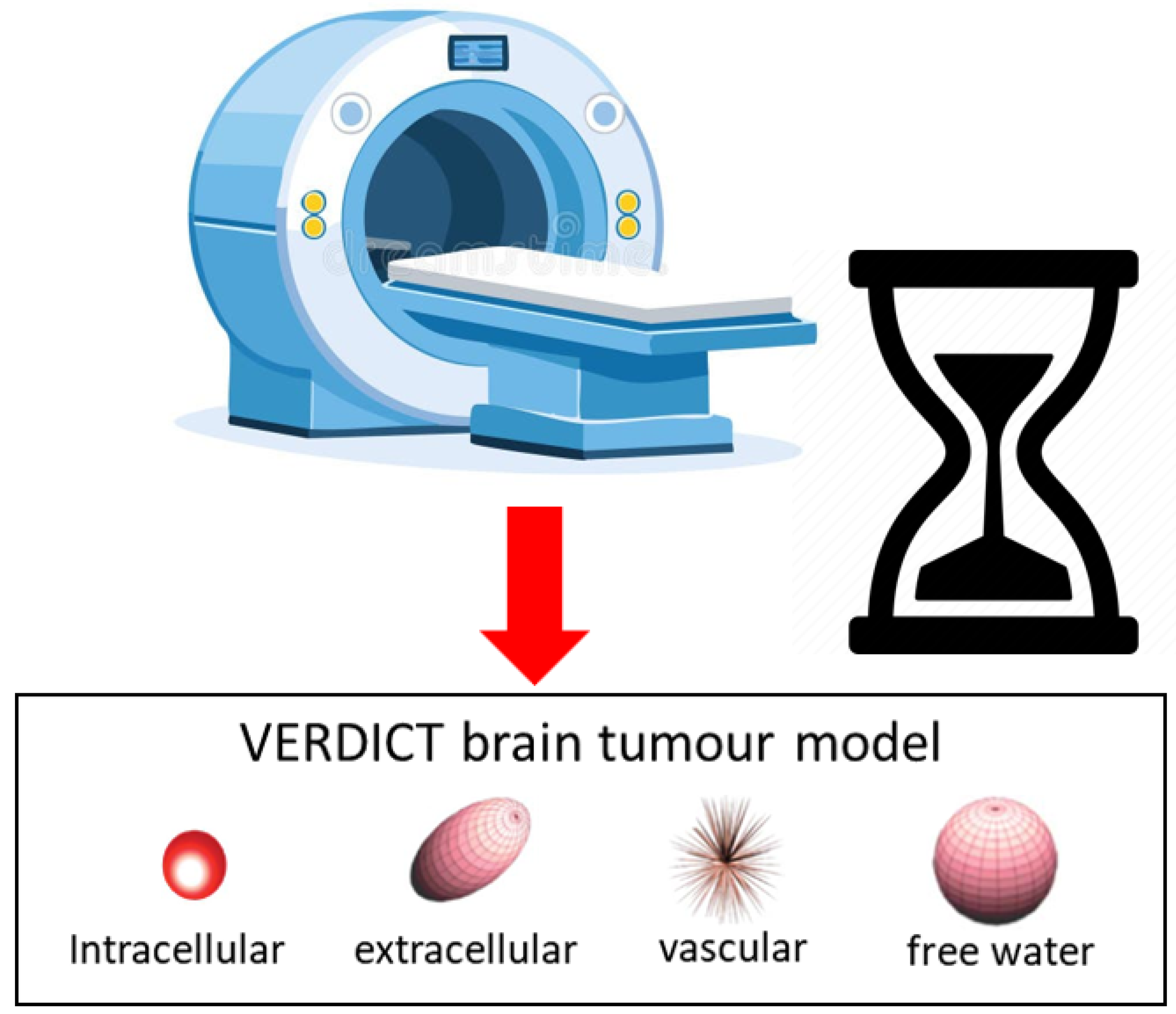
Figure 3.
Overall performance comparison across all architectures.
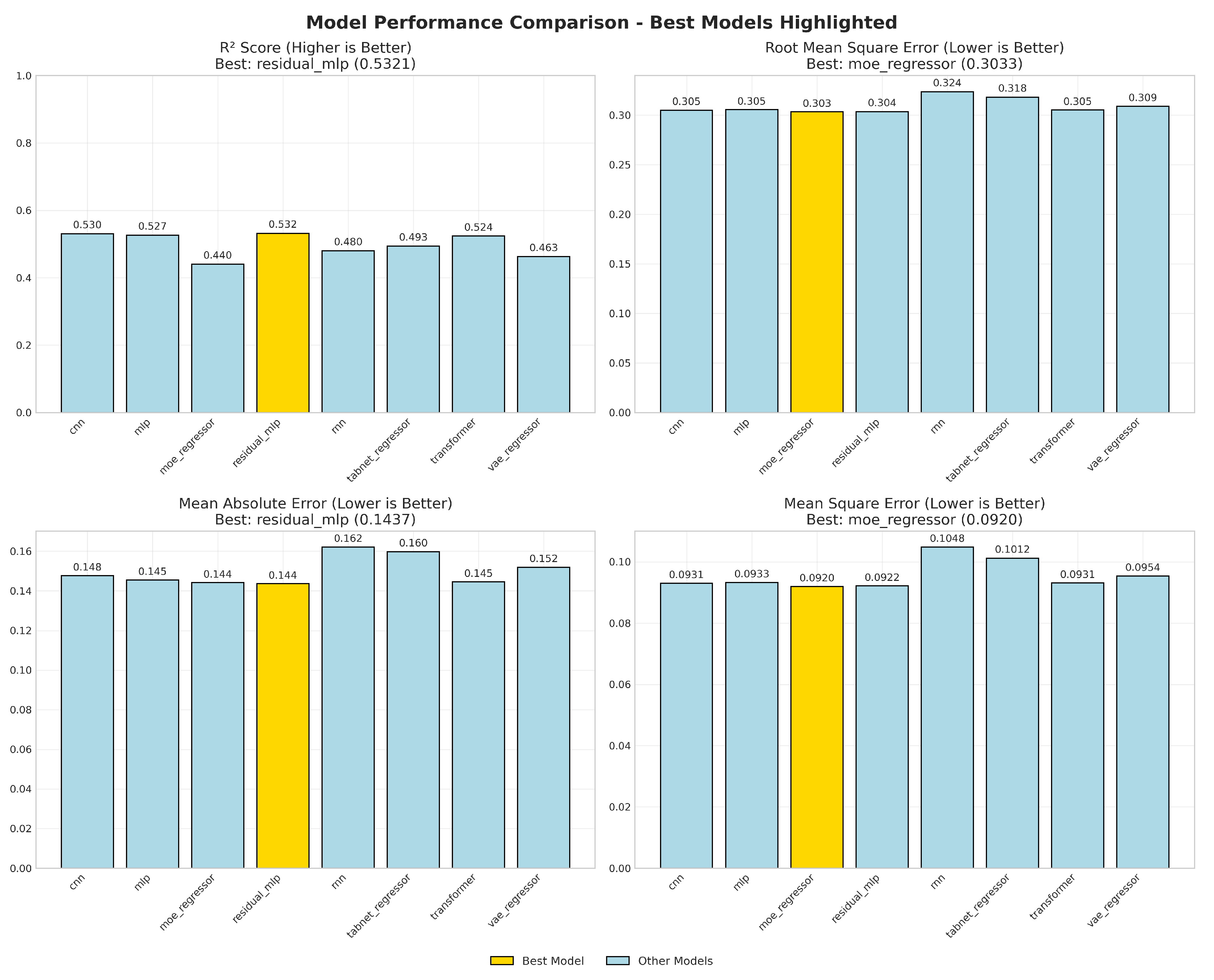
Figure 4.
95% bootstrap confidence intervals (1000 resamples) for primary metrics. The best model per metric is highlighted.
Figure 4.
95% bootstrap confidence intervals (1000 resamples) for primary metrics. The best model per metric is highlighted.
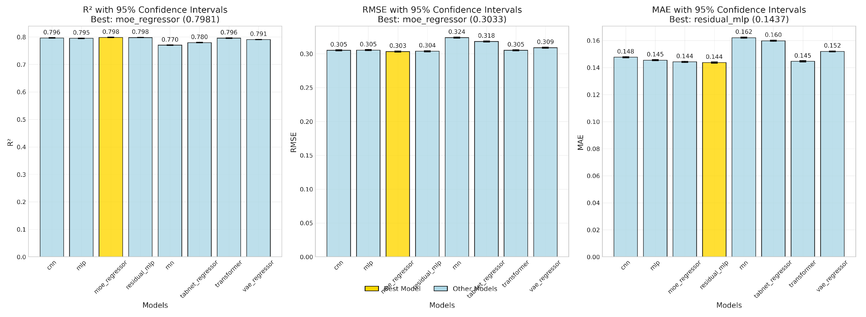
Figure 5.
Correlation heatmap summarizing parameter-wise relationships. Warmer colours denote stronger positive correlation.
Figure 5.
Correlation heatmap summarizing parameter-wise relationships. Warmer colours denote stronger positive correlation.
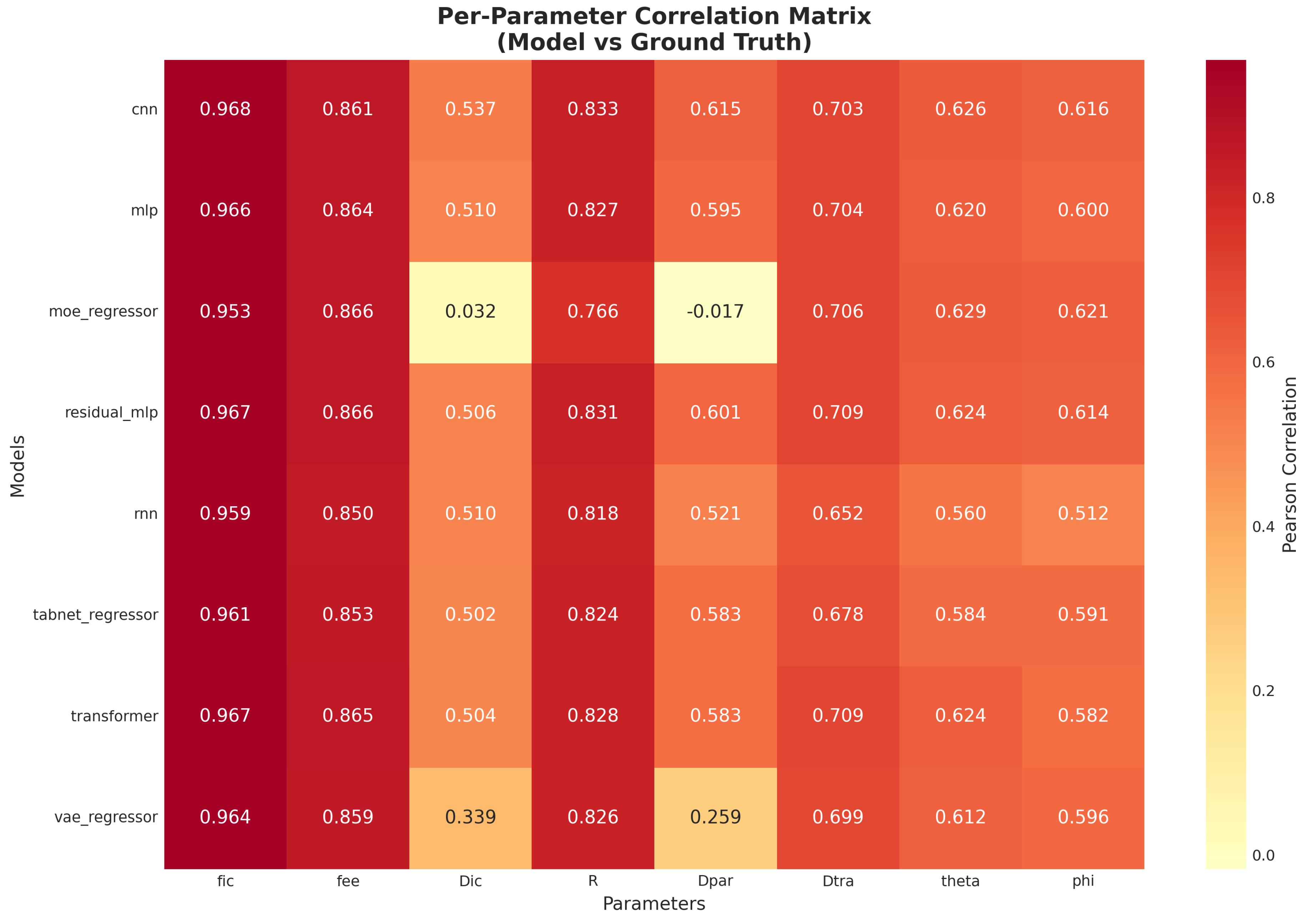
Figure 6.
Error distributions across parameters. Narrow, symmetric distributions centered at zero reflect stable estimators.
Figure 6.
Error distributions across parameters. Narrow, symmetric distributions centered at zero reflect stable estimators.
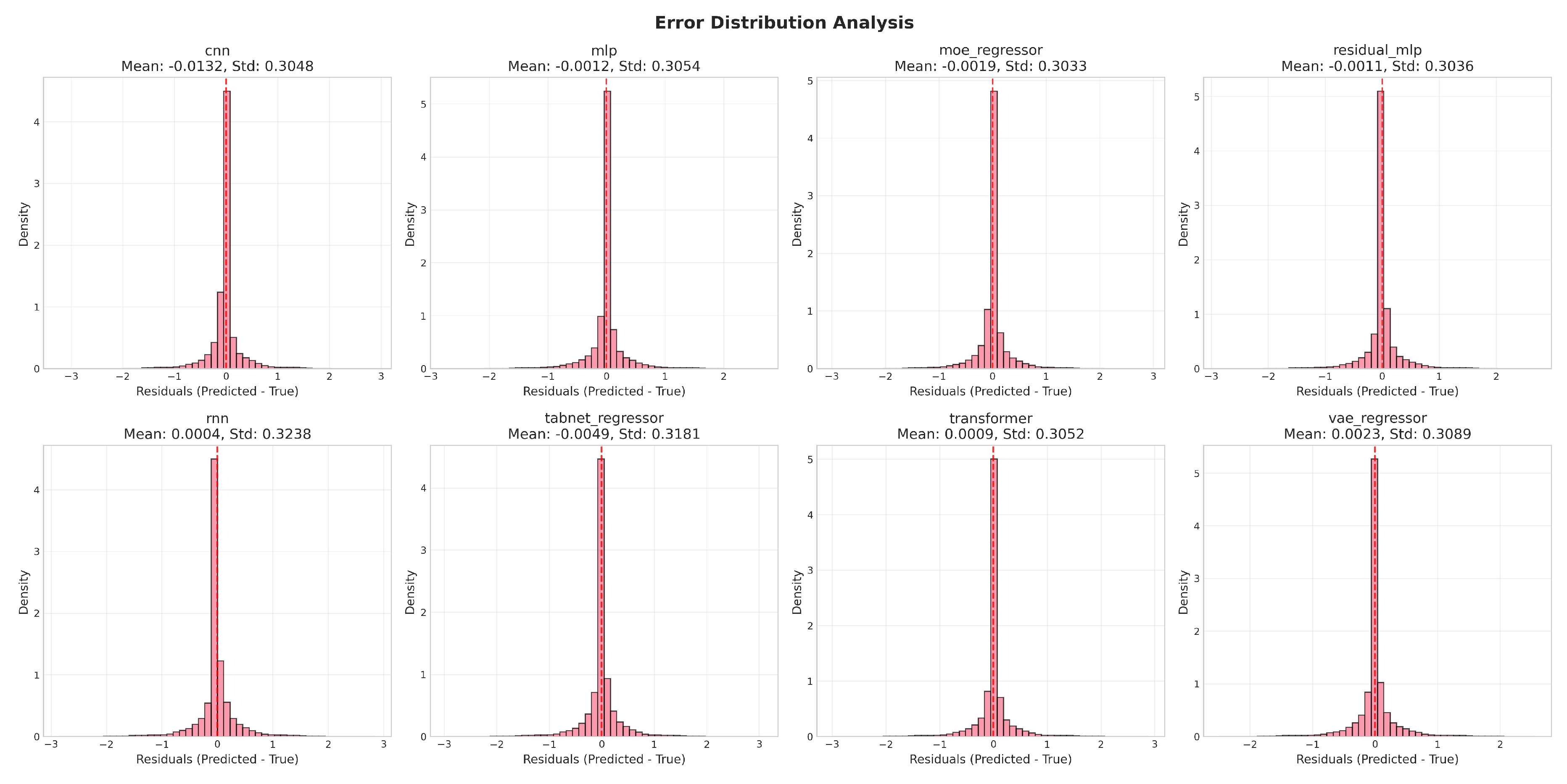
Figure 7.
Training loss. Early stopping prevents overfitting once validation loss ceases to improve.
Figure 7.
Training loss. Early stopping prevents overfitting once validation loss ceases to improve.
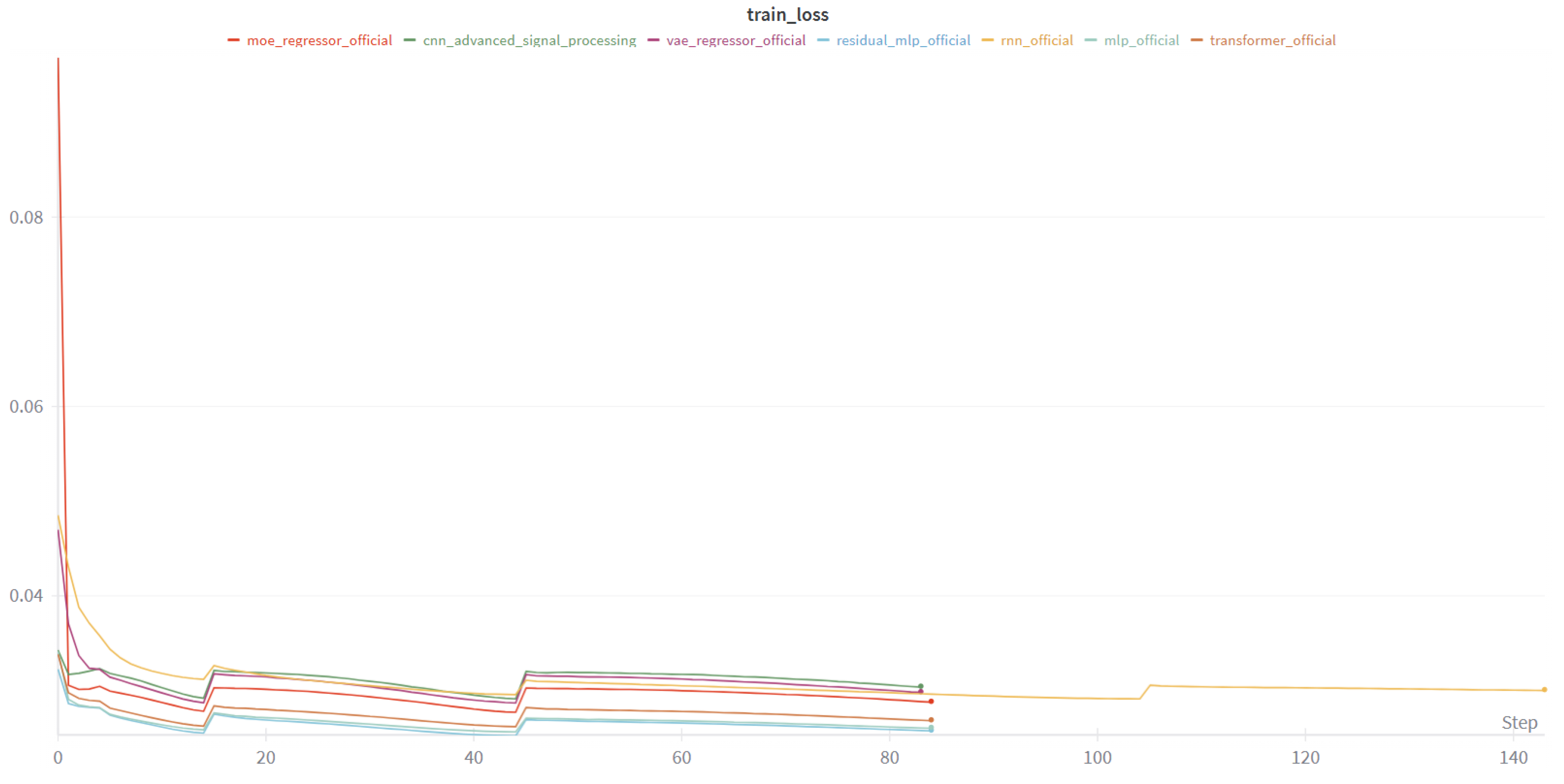
Figure 8.
Validation loss. Early stopping prevents overfitting once validation loss ceases to improve.
Figure 8.
Validation loss. Early stopping prevents overfitting once validation loss ceases to improve.
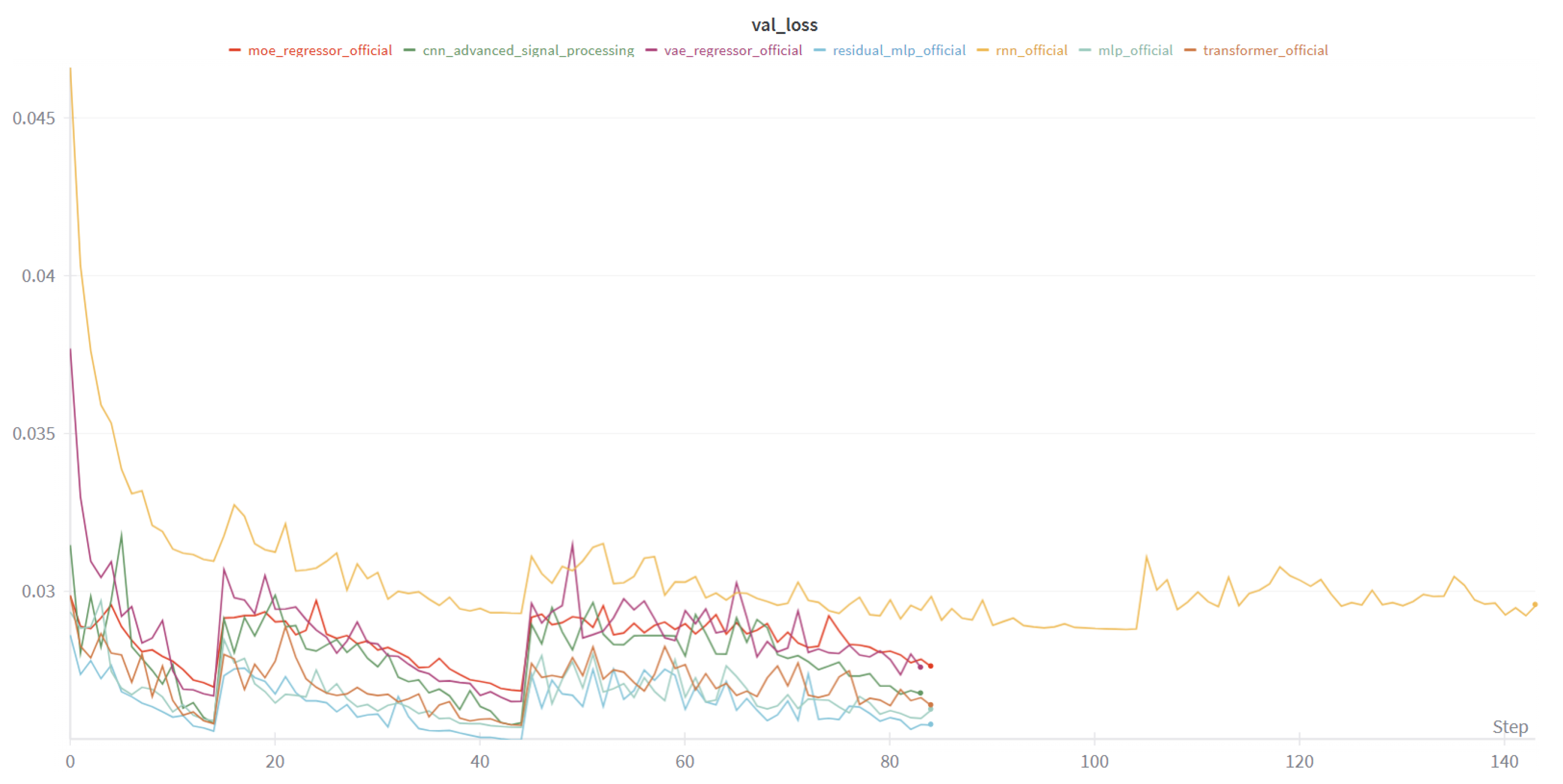
Figure 9.
Model complexity vs. performance. Trend lines fitted via simple least-squares.
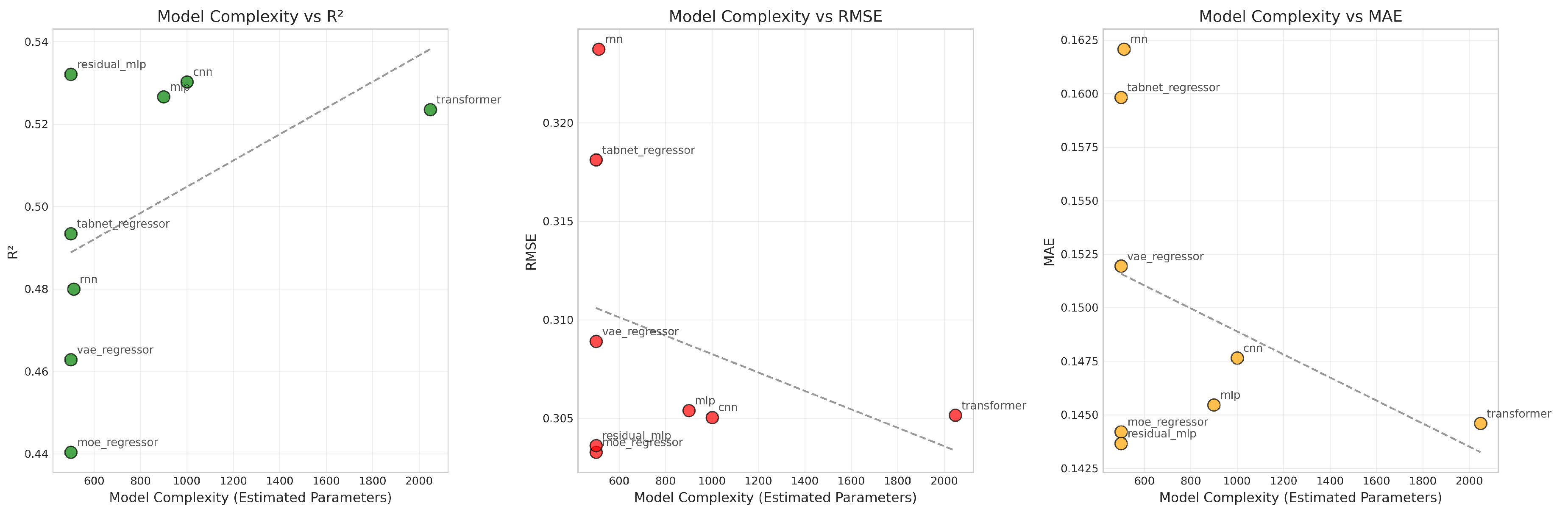
Figure 10.
Parameter maps () for three patients at central brain slices. Tumour regions (leftmost column) are highlighted and compared across VERDICT parameters.
Figure 10.
Parameter maps () for three patients at central brain slices. Tumour regions (leftmost column) are highlighted and compared across VERDICT parameters.
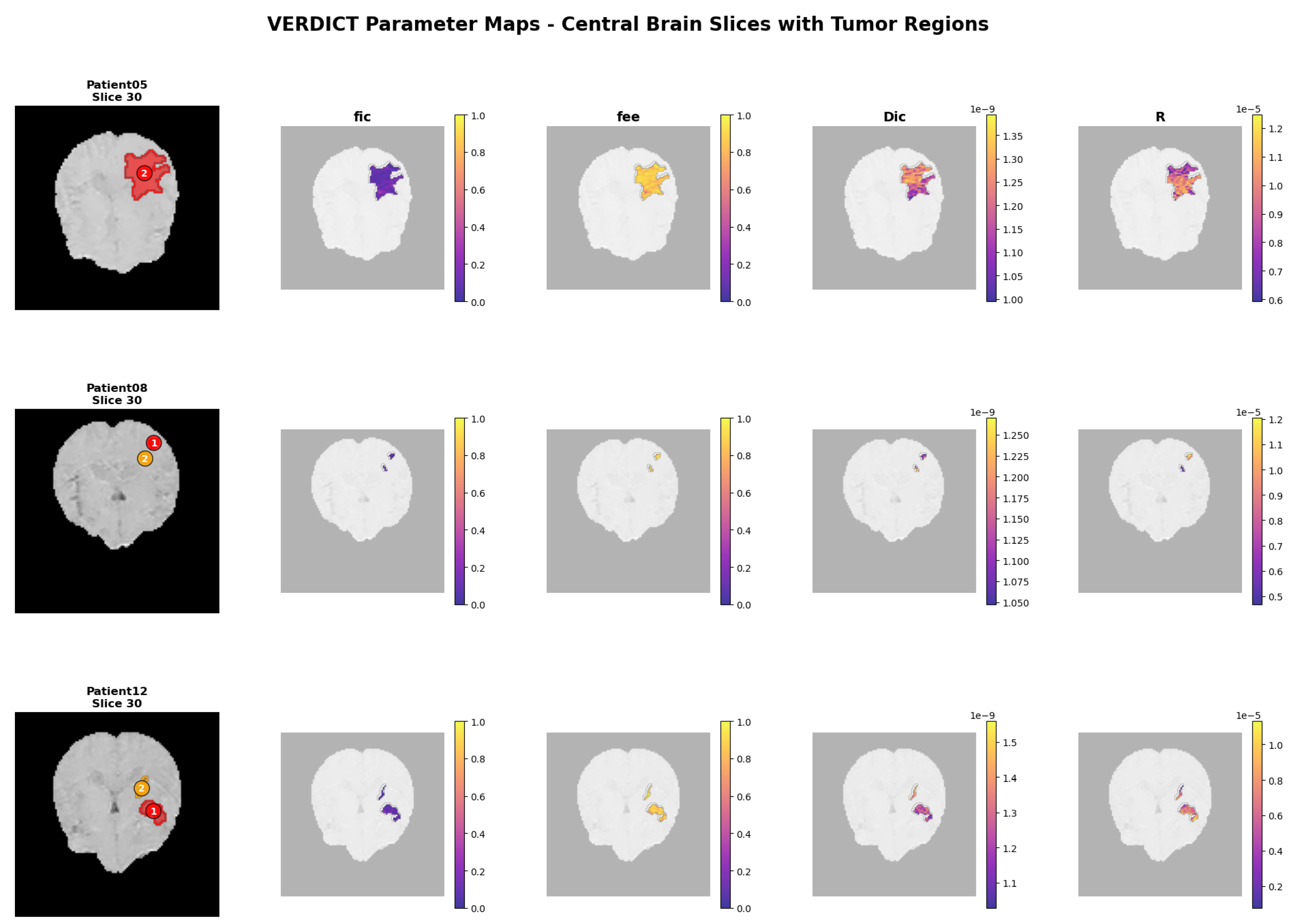
Figure 11.
Model-level VERDICT reconstructions (Part 1: CNN, MLP, ResNet, MoE).
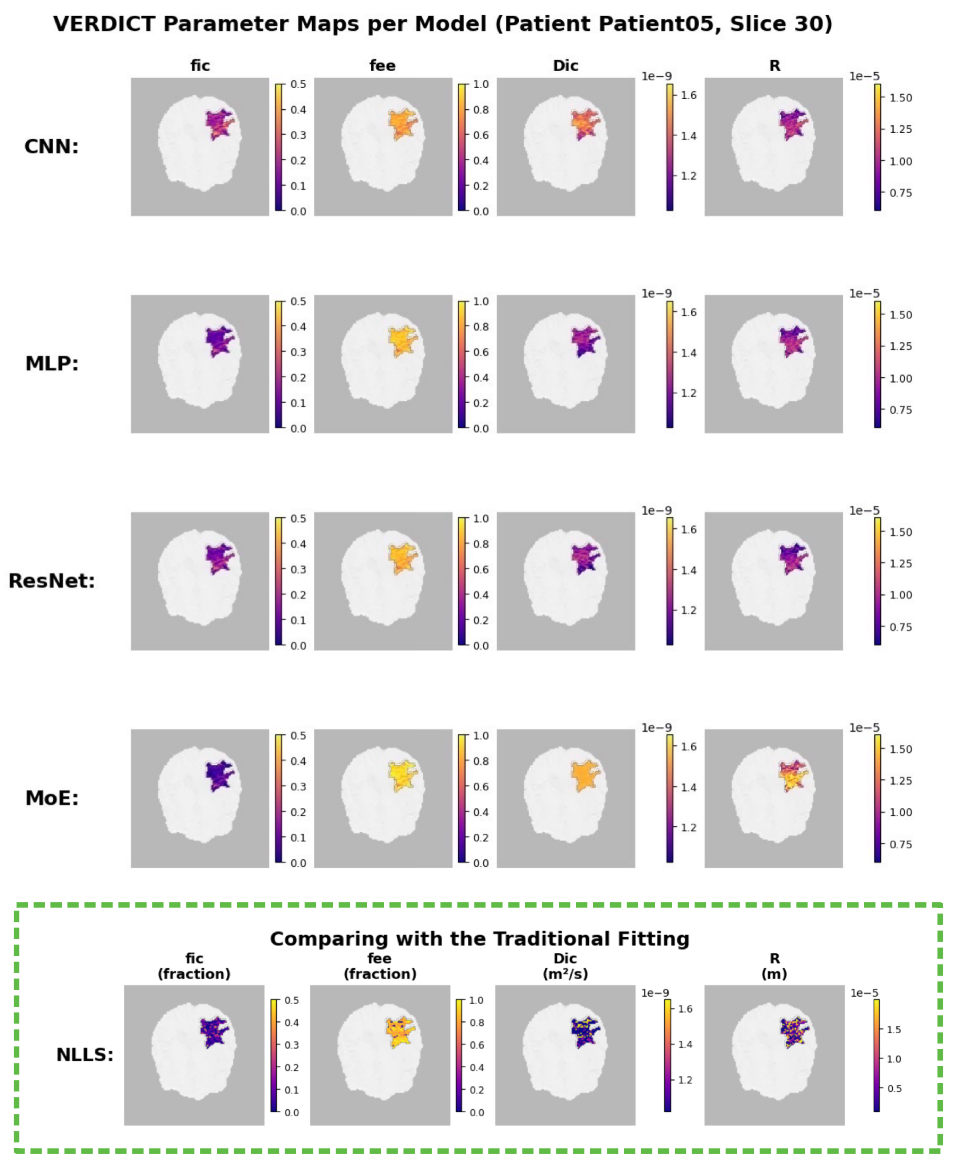
Figure 12.
Model-level VERDICT reconstructions (Part 2: RNN, TabNet, Transformer, VAE).
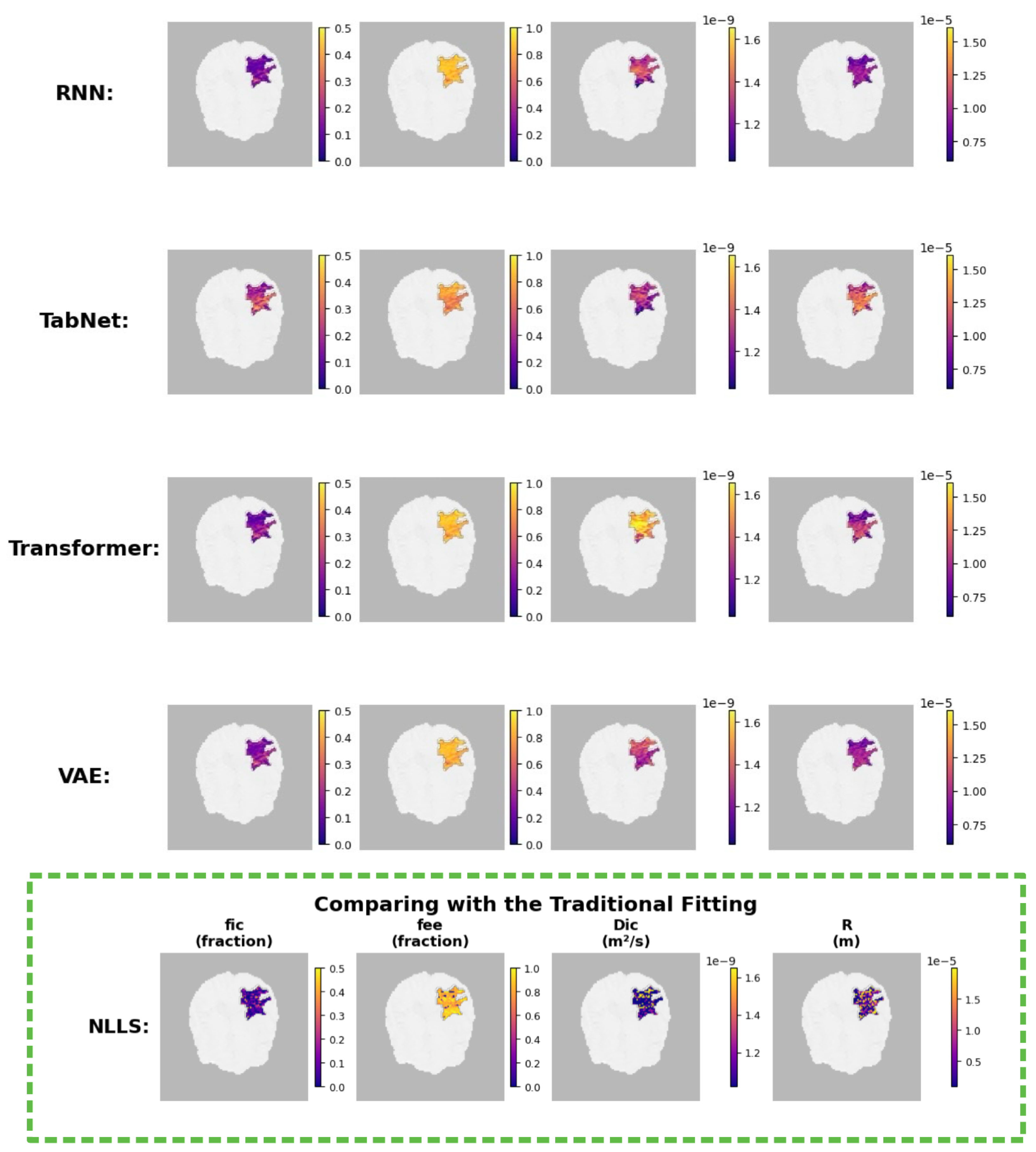
Figure 13.
distribution comparison between WHO Grade 2 (red) and Grade 4 (blue) across eight neural network architectures.
Figure 13.
distribution comparison between WHO Grade 2 (red) and Grade 4 (blue) across eight neural network architectures.
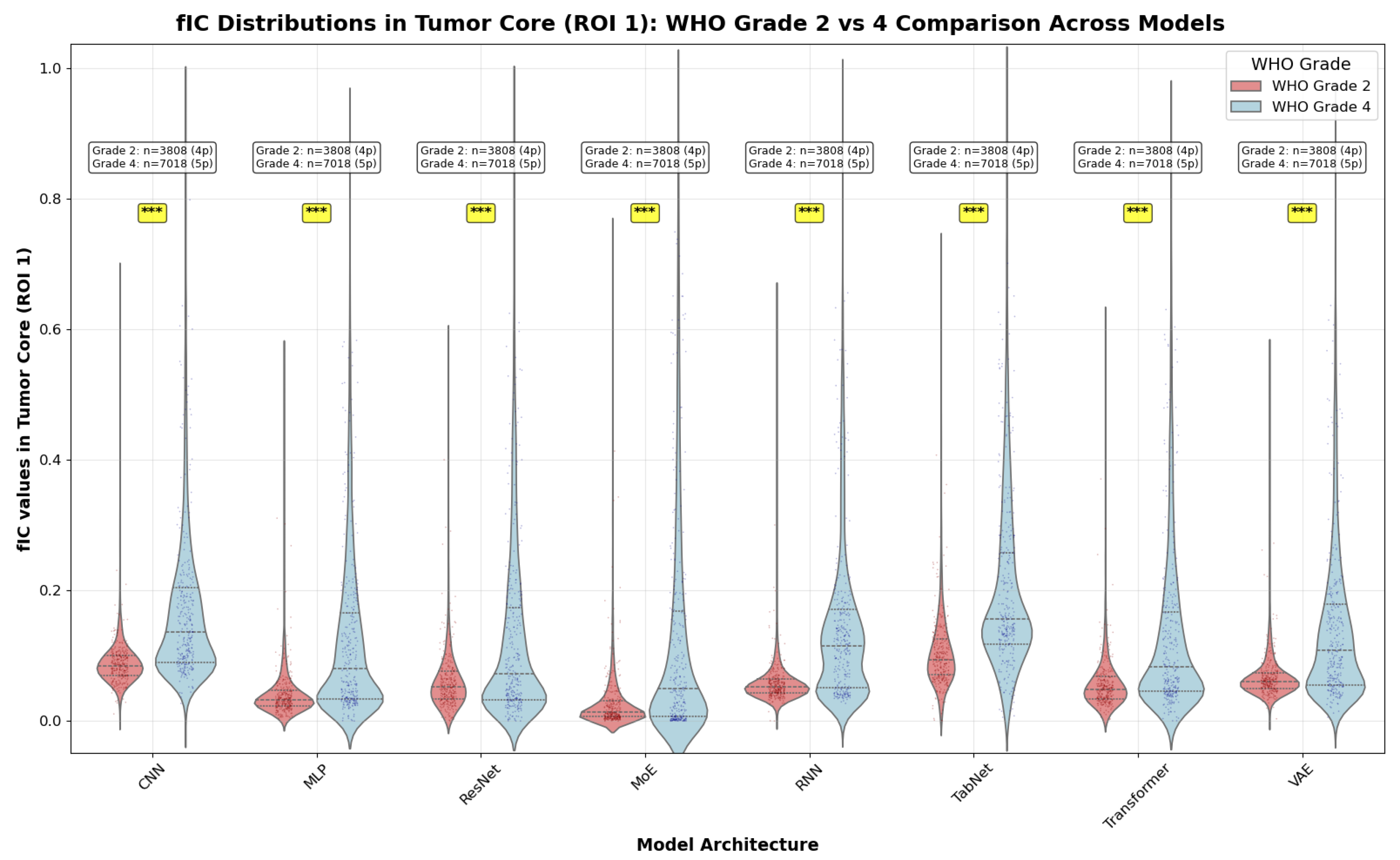
Figure 14.
distribution comparison between WHO Grade 2 (red) and Grade 3 (green) across eight neural network architectures.
Figure 14.
distribution comparison between WHO Grade 2 (red) and Grade 3 (green) across eight neural network architectures.
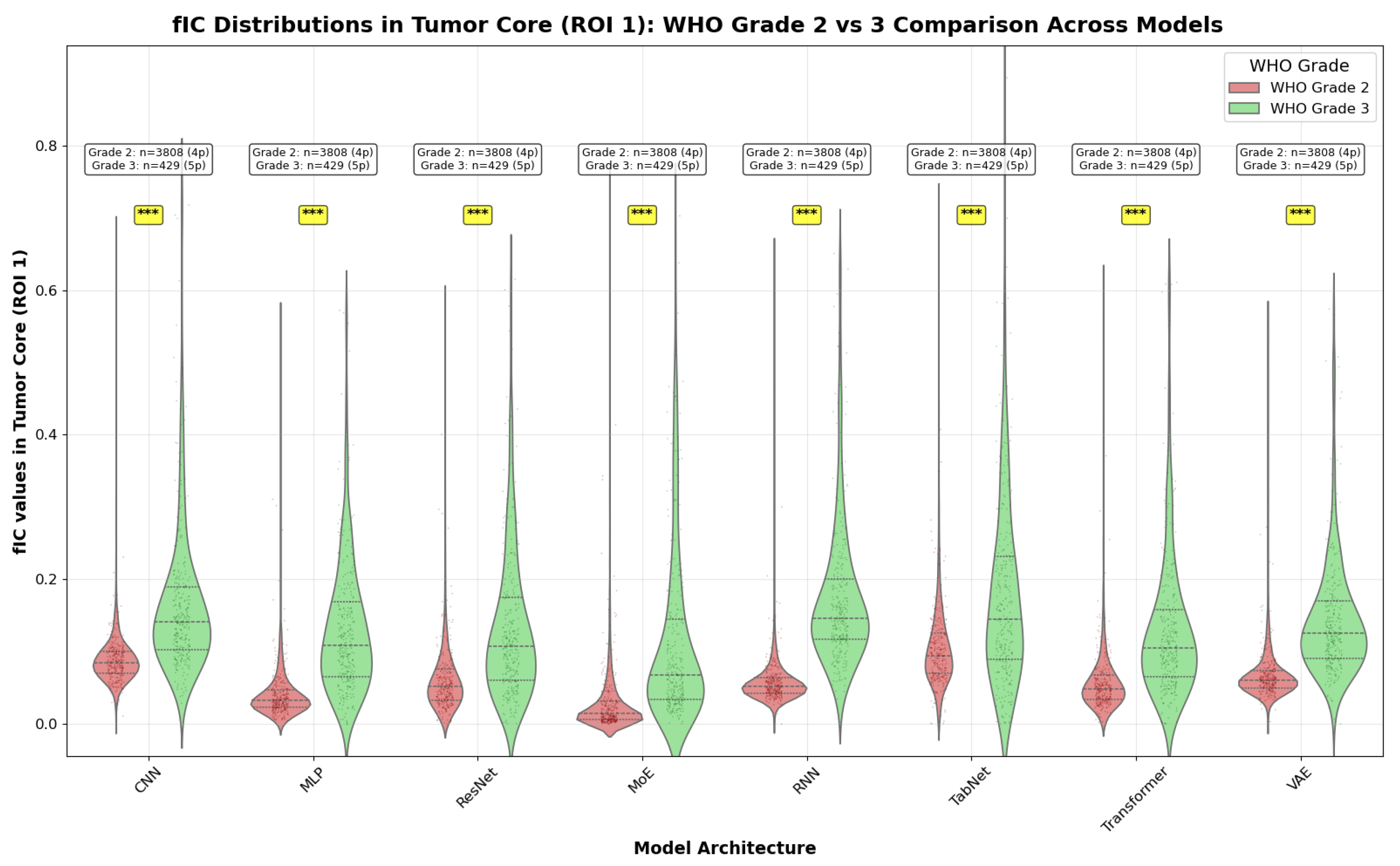
Figure 15.
distribution comparison between WHO Grade 3 (green) and Grade 4 (blue) across eight neural network architectures.
Figure 15.
distribution comparison between WHO Grade 3 (green) and Grade 4 (blue) across eight neural network architectures.
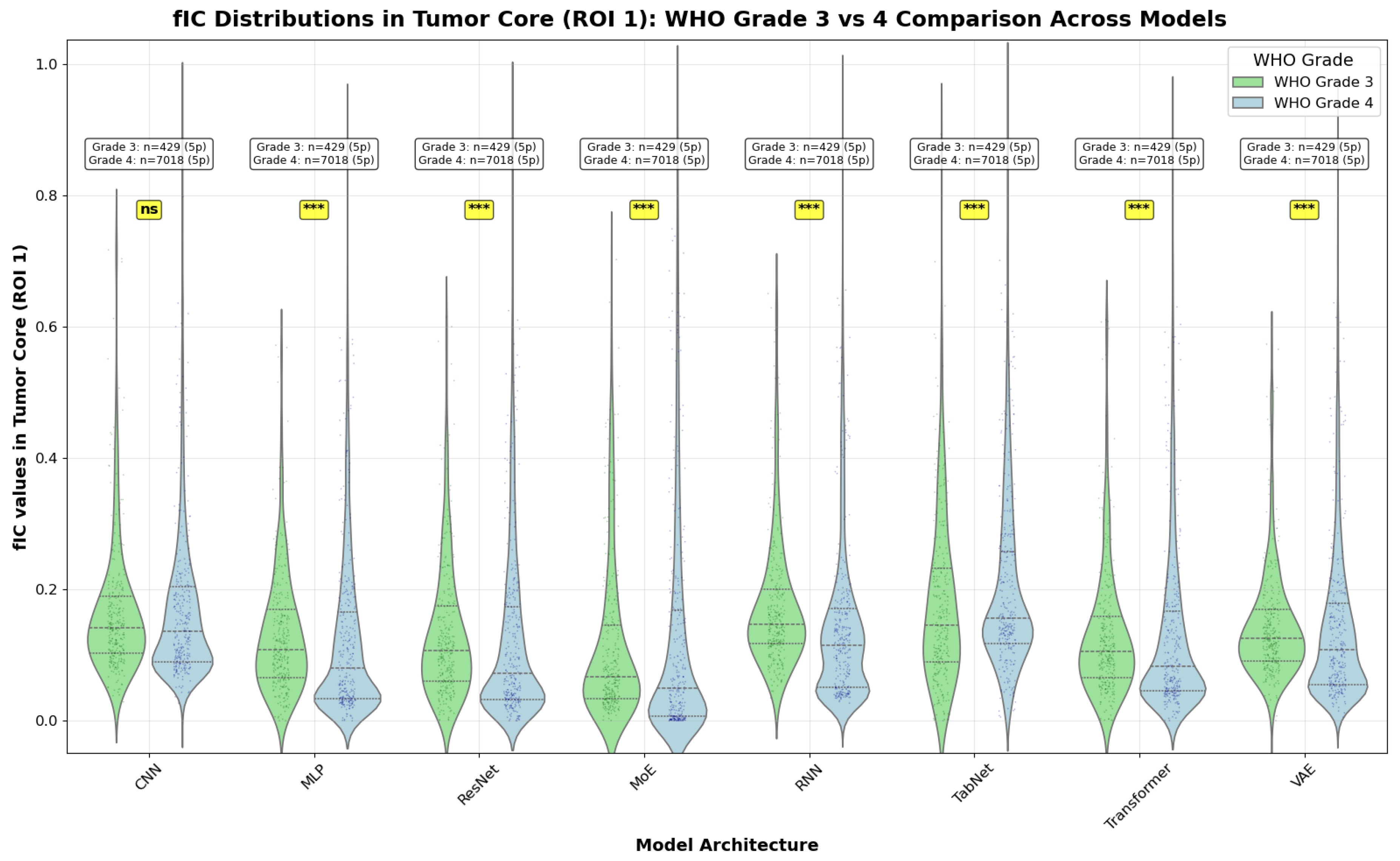
Figure 16.
Heatmap overview of three effect size metrics: Cohen’s d (left), Glass’s (middle), and Cliff’s (right): for each model architecture (rows) and WHO grade pair (columns). Darker hues indicate larger absolute effect sizes (stronger separation), with blue tones representing negative differences (e.g., higher in the higher-grade group) and orange tones representing positive differences. The RNN shows the largest |effect size| for Grade 2 vs 3 across all three metrics, Grade 2 vs 4 yields uniformly large effects across models, and Grade 3 vs 4 generally exhibits only low to moderate effects with variability across architectures.
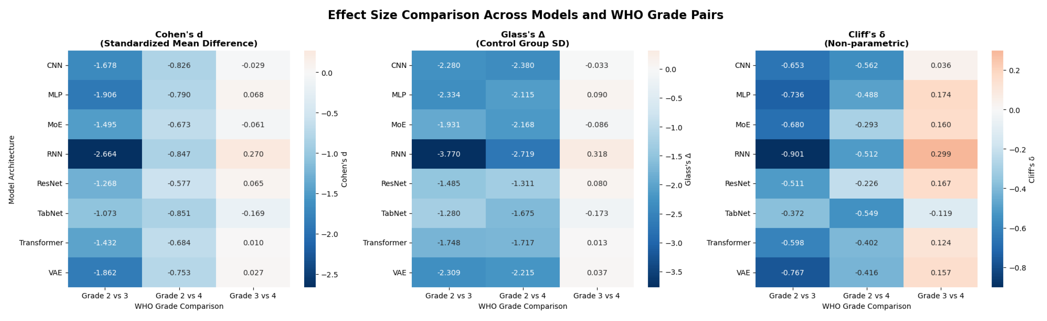
Figure 17.
Cohen’s d by model for Grade 2 vs 3 (blue), Grade 2 vs 4 (orange), and Grade 3 vs 4 (green). Dashed horizontal lines mark conventional thresholds for small (), medium (), and large () effects [48]. All models achieve large effects for Grade 2 vs 3 and medium-to-large effects for Grade 2 vs 4, while Grade 3 vs 4 is typically small. The RNN attains the largest for Grade 2 vs 3 and a small-but-clear effect for Grade 3 vs 4 relative to other models.
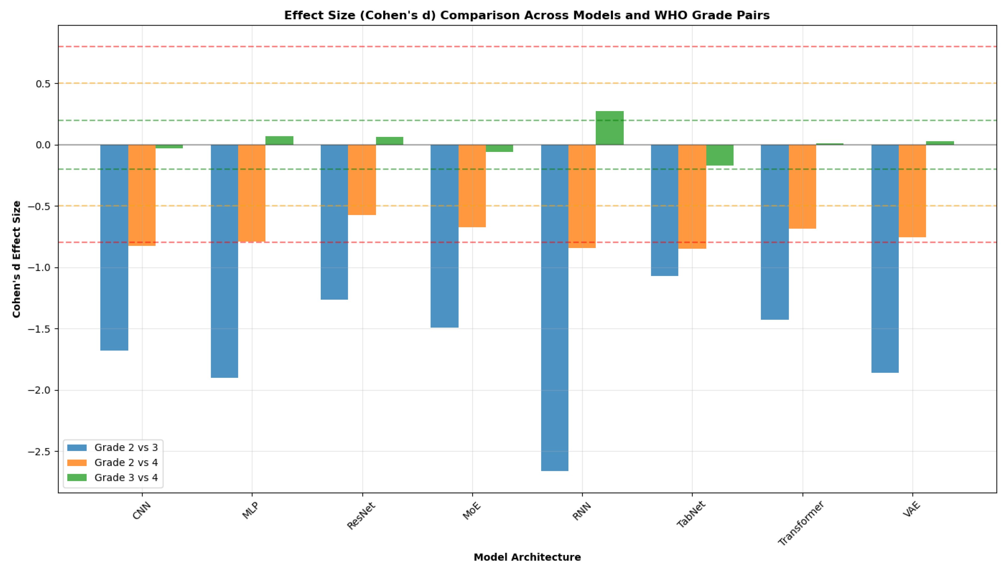

Table 1.
Acquisition parameters for the dMRI protocol. Abbreviations: b = b-value (degree of diffusion weighting), TE = echo time, = diffusion gradient duration, = diffusion gradient separation, Ndir = number of diffusion gradient directions.
Table 1.
Acquisition parameters for the dMRI protocol. Abbreviations: b = b-value (degree of diffusion weighting), TE = echo time, = diffusion gradient duration, = diffusion gradient separation, Ndir = number of diffusion gradient directions.
| b (s/mm2) | 50 | 70 | 90 | 110 | 350 | 1000 | 1500 | 2500 | 3000 | 3500 | 711 | 3000 |
| TE (ms) | 45 | 53 | 43 | 43 | 54 | 78 | 118 | 88 | 103 | 123 | 78 | 78 |
| (ms) | 5 | 5 | 5 | 5 | 10 | 10 | 10 | 20 | 15 | 15 | 20 | 20 |
| (ms) | 22 | 30 | 20 | 20 | 26 | 50 | 90 | 50 | 70 | 90 | 42 | 42 |
| Ndir | 3 | 3 | 3 | 3 | 3 | 3 | 3 | 3 | 3 | 3 | 38 | 63 |
Table 2.
Parameter ranges used to generate synthetic training/validation data (per acquisition scheme). Diffusivities are in ; R in meters.
Table 2.
Parameter ranges used to generate synthetic training/validation data (per acquisition scheme). Diffusivities are in ; R in meters.
| Parameter | min | max |
|---|---|---|
| 0 | ||
| 0 | ||
| R () | ||
| () | ||
| () | ||
| () | 0 | 1 |
| () | 0 | |
| () | 0 |
Table 3.
Patient05 VERDICT parameter summary (mean ± SD). Units: diffusivities in /ms; radius in m; angles in rad.
Table 3.
Patient05 VERDICT parameter summary (mean ± SD). Units: diffusivities in /ms; radius in m; angles in rad.
| Parameter | Tumour core (2 voxels) | Peritumoural area (6202 voxels) |
| Cell density | ||
| Extracellular | ||
| Cell diffusivity | ||
| Cell radius R | ||
| Parallel diffusivity | ||
| Transverse diffusivity | ||
| Polar angle | ||
| Azimuthal angle |
Clinical insights: Tumour core shows higher cellularity (: vs ); cell sizes R: Tumour core , Peritumoural area ( for Tumour core).
Table 4.
Patient 8 VERDICT parameter summary (mean ± SD). Units: diffusivities in /ms; radius in m; angles in rad.
Table 4.
Patient 8 VERDICT parameter summary (mean ± SD). Units: diffusivities in /ms; radius in m; angles in rad.
| Parameter | Tumour core (1040 voxels) | Peritumoural area (50 voxels) |
| Cell density | ||
| Extracellular | ||
| Cell diffusivity | ||
| Cell radius R | ||
| Parallel diffusivity | ||
| Transverse diffusivity | ||
| Polar angle | ||
| Azimuthal angle |
Clinical insights: Peritumoural area shows higher cellularity ( vs ); cell sizes R: Tumour core , Peritumoural area (Tumour core larger by ).
Table 5.
Patient 12 VERDICT parameter summary (mean ± SD). Units: diffusivities in /ms; radius in m; angles in rad.
Table 5.
Patient 12 VERDICT parameter summary (mean ± SD). Units: diffusivities in /ms; radius in m; angles in rad.
| Parameter | Tumour core (1230 voxels) | Peritumoural area (606 voxels) |
| Cell density | ||
| Extracellular | ||
| Cell diffusivity | ||
| Cell radius R | ||
| Parallel diffusivity | ||
| Transverse diffusivity | ||
| Polar angle | ||
| Azimuthal angle |
Clinical insights: Tumour core shows higher cellularity ( vs ); cell sizes R: Tumour core , Peritumoural area (Peritumoural area larger by ).
Disclaimer/Publisher’s Note: The statements, opinions and data contained in all publications are solely those of the individual author(s) and contributor(s) and not of MDPI and/or the editor(s). MDPI and/or the editor(s) disclaim responsibility for any injury to people or property resulting from any ideas, methods, instructions or products referred to in the content. |
© 2026 by the authors. Licensee MDPI, Basel, Switzerland. This article is an open access article distributed under the terms and conditions of the Creative Commons Attribution (CC BY) license (http://creativecommons.org/licenses/by/4.0/).
Copyright: This open access article is published under a Creative Commons CC BY 4.0 license, which permit the free download, distribution, and reuse, provided that the author and preprint are cited in any reuse.


