Submitted:
31 January 2026
Posted:
03 February 2026
You are already at the latest version
Abstract
The structure of the direct electrical current in a conductor is discussed neither in the educa-tional nor scientific literature. This problem is directly related to the boundary condition for thenormal component of current density. The generally accepted approach to this problem requiresmore careful consideration. The following article is devoted to the analysis of the direct current dis-tribution in a conductor. In this paper, we consider two mutually exclusive approaches to explainthe structure of direct current in a conductor.
Keywords:
surface charge distribution
; conductors
; electric current
; electrodynamics
1. Introduction
It is generally accepted in physics that normal current density component at the conductor boundary with a non-conductive medium is zero. An elementary proof of this assumption is based on the continuity equation (law of conservation of electric charge). Owing to the potentiality of the electric field and the proportionality of current density to electrostatic field intensity (for simplicity, we assume a cylindrical conductor), the generated homogeneous electric current is directed along the axis of the conductor.
The flaw in this proof is as follows. The generally accepted boundary condition, which is stated in [1], says that the charges are distributed over the surface of the conductor and create a field that leads to the directed movement of electrons.
Evidently the distribution of charges over the surface of the conductor should be heterogeneous. Field lines originate on positive charges and terminate on negative charges (Fig. 1). Under the generally accepted boundary condition, field lines bypass the charges that are the sources of the field. This does not support the generally accepted approach. Figure 1 depicts that is not equal zero.
2. Field Inside a Cylindrical Conductor
The normal component of the current density being equal to zero is possible only in the absence of near-surface current, the value of which decreases with approaching to the middle of cylindrical conductor. Surface charges that create the field are also moving, but the resultant surface current is negligible.
What is this near-surface current? The existence of a normal component of the current density near the surface of the conductor leads to the appearance of an uncompensated charged, which causes the appearance of a near-surface relaxation current.
The relaxation time constant, as stated in [2], is , where is conductivity. Toward the middle of the conductor, the surface current decreases and the volume current increases, reaching a maximum. To describe this process, we must use a more complicated boundary condition: instead of (where is the value of near-surface current, z is parallel to the axis of the cylinder coordinate, and a is the radius of the cylindrical conductor). Note that there is no such distribution in the surface charge density for the cylindrical conductor, which leads to the creation of a uniform field inside it.
Next, we obtain the potential of the electric field inside the cylindrical conductor at point created by charge located at point (Fig. 2).
The surface charge has an axisymmetric distribution:
where surface charge density is expressed using linear density :
After a series of simple transformations, Eq. (1) can be reduced to the following form:
where , , , and . The expression can be expanded into a series using the Legendre polynomials:
where , , . Integrating Eq. (3) over in the range from 0 to , we obtain
Assuming that and integrating over from to , we obtain
where .
Using Eq. (6), it is possible to obtain expressions for the longitudinal and transverse components of the electric field intensity in the conductor, as well as the approximate value of . In particular, away from the ends of the conductor,
where is the total current flowing through the conductor. The results obtained here suggest that the generally accepted boundary condition needs to be revised.
3. Field Inside a Conducting Ball
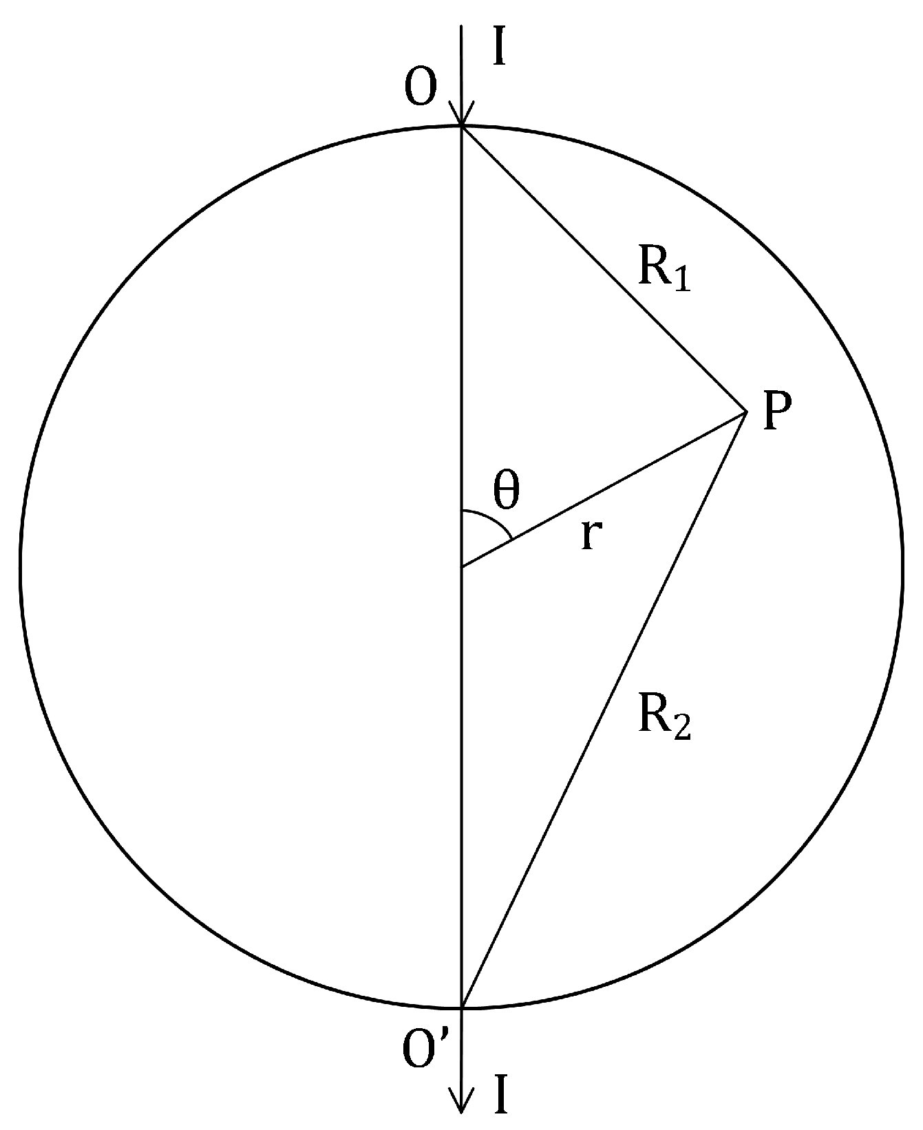
Let us determine the distribution of the potential of the electric field in a conducting ball. Current I enters through one pole (point O) and exits through the opposite pole (point ) (Fig. 3).
The solution to a similar problem is given in [3]. However, the boundary condition used to solve this problem was , where a is the radius of the ball. Surface current leads to the following boundary condition:
The use of this boundary condition significantly affects the determination of the electric potential, which at an arbitrary point P inside the ball can be represented as
Using the transformations associated with the expansion in Legendre polynomials, we obtain
Substituting Eq. (12) into Eq. (10), we obtain an expansion in terms of . If we equate the coefficients of to zero, we obtain a system of equations for calculating . In the third approximation, we obtain
and in the fifth approximation,
Furthermore,
which correspond to a uniform field inside the ball with intensity
It is easy to demonstrate that
Summarizing the results of the coefficient calculations, we get
and
for the values of the electric field intensity obtained in Eqs. (15) and (16).
It is interesting to note that the bulk current will be equal to
and the near-surface current will be
4. Conclusions
The inhomogeneous distribution of the surface charge leads to the conclusion that the normal component of the current density is nonzero. Near-surface and bulk currents appear in the conductor, changing their magnitude along the conductor axis. The near-surface current has a relaxing nature. In the case of a cylindrical conductor, an approximate calculation of the current density and electric field intensity (far from its ends and near its axis) has been done. An exact expression is obtained for the bulk and near-surface currents in a conducting ball. It is demonstrated that the electric field inside the ball is uniform.
References
- Papalexi, N. D. The Course of Physics (1942); Vol. 2.
- Panofsky, W. K. H.; Phillips, M. Classical Electricity and Magnetism, 2nd ed.; Addison-Wesley, 1962. [Google Scholar]
- Landau, L. D.; Lifshitz, E. M. Electrodynamics of Continuous Media, 2nd ed.; 1984. [Google Scholar]
Figure 1.
Field lines.
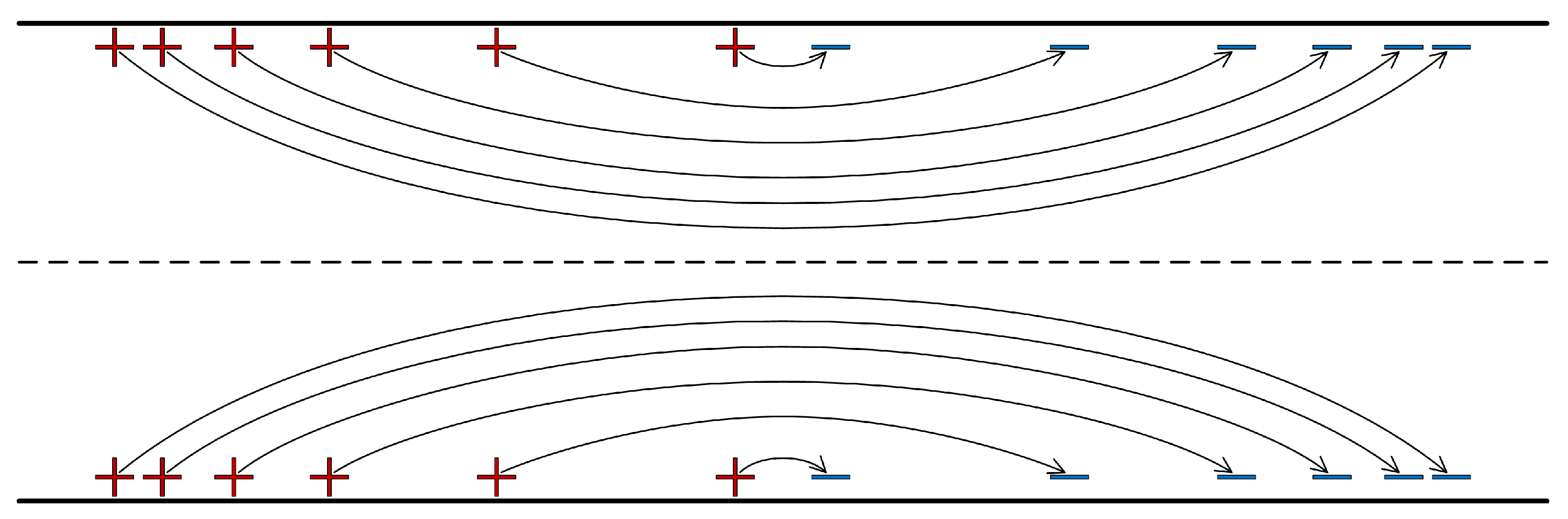
Figure 2.
Calculation of electric potential in a cylindrical conductor.
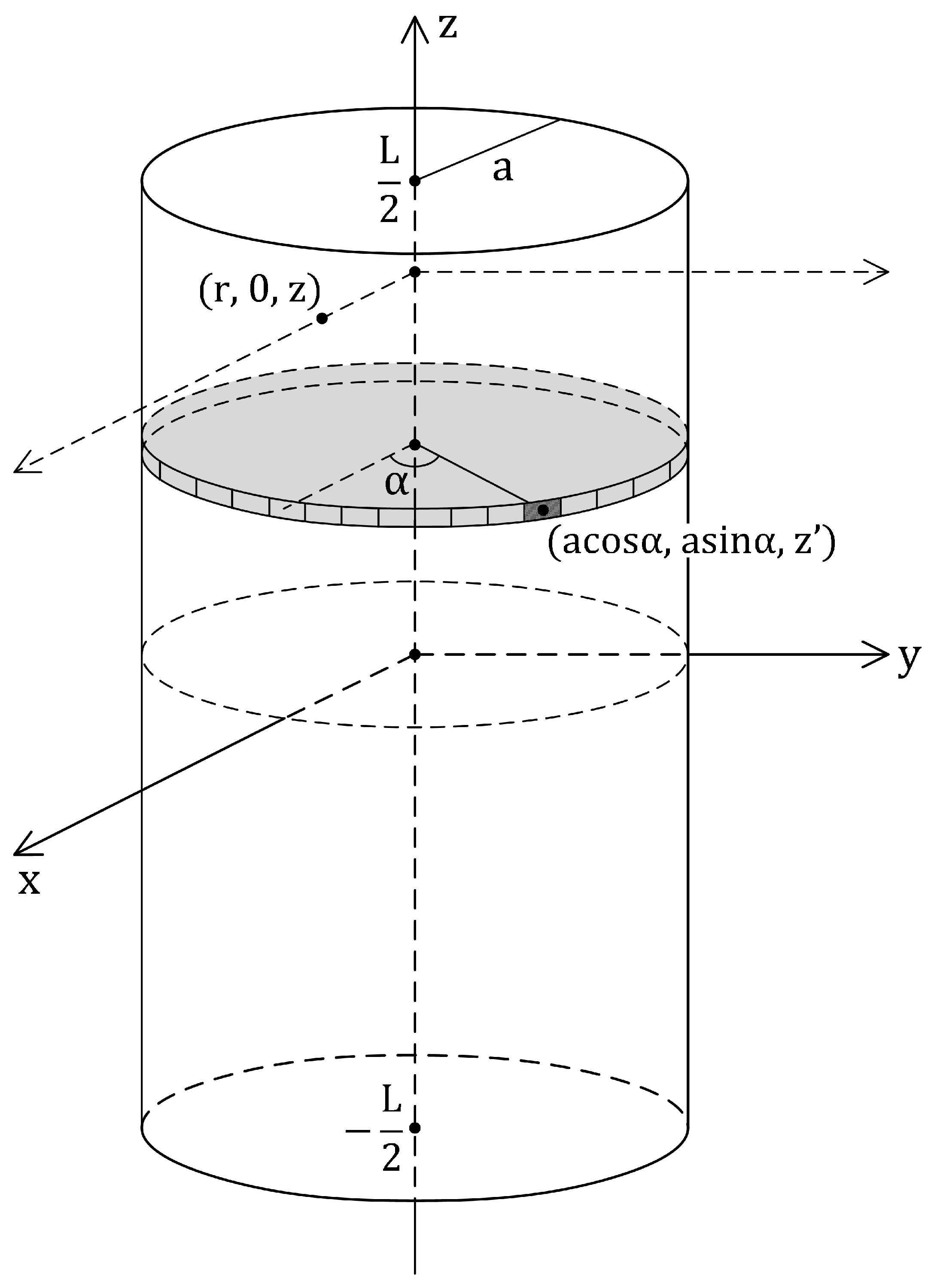
Figure 3.
Calculation of electric potential in a conducting ball.
Disclaimer/Publisher’s Note: The statements, opinions and data contained in all publications are solely those of the individual author(s) and contributor(s) and not of MDPI and/or the editor(s). MDPI and/or the editor(s) disclaim responsibility for any injury to people or property resulting from any ideas, methods, instructions or products referred to in the content. |
© 2026 by the authors. Licensee MDPI, Basel, Switzerland. This article is an open access article distributed under the terms and conditions of the Creative Commons Attribution (CC BY) license (http://creativecommons.org/licenses/by/4.0/).
Copyright: This open access article is published under a Creative Commons CC BY 4.0 license, which permit the free download, distribution, and reuse, provided that the author and preprint are cited in any reuse.


