
Submitted:
02 February 2026
Posted:
03 February 2026
You are already at the latest version
Abstract
Introduction: High Andean lagoons in southern Peru have critical hydrological and ecological functions; however, long-term time series integrating trophic, integral quality, and metal contamination metrics to support adaptive management are lacking. Methods: A total of 1,846 records (2015–2024) from four systems (3,100–4,600 m asl) were analyzed using seven indices (CTSI, TRIX, OWQI, WQIHA, CCME-WQI, HPI, and CD). Temporal trends were assessed by using Mann–Kendall and Theil–Sen slope; spatial heterogeneity using Kruskal–Wallis and Dunn–Bonferroni comparisons; controlling factors using distance-based redundancy analysis (999 permutations); and functional typology using Ward's hierarchical clustering on Z-standardized data. Results: 97% of the series lacked monotonic trends, demonstrating high interannual stability; spatial variance was marked (ε² = 0.73 in CCME-WQI). db-RDA explained 24.6% of the total variability by lake identity, year, and wet-dry period. Four functional archetypes emerged, including a metal-eutrophic hotspot (HPI ≈ 213; CD ≈ 25 µg L⁻¹) and recovering reservoirs with CCME-WQI ≈ 63. CTSI thresholds ≥ 60 combined with HPI ≥ 100 signaled the transition to cyanobacterial dominance. Conclusions: Systems show temporal resilience but strong spatial divergence induced by local pressures; The proposed typology and thresholds provide an operational basis for early warnings and prioritization of remediation actions in high-mountain ecosystems subject to increasing anthropogenic stress.
Keywords:
multivariate analysis
; heavy metal contamination
; trophic status
; adaptive management
; multimetric water quality indices
; high Andean lagoons
1. Introduction
Lakes and reservoirs store approximately 87% of the Earth's liquid fresh surface water and support critical functions—drinking, irrigation, climate regulation, and hydropower generation—for more than three billion people. However, a warming climate and increasing anthropogenic pressures are accelerating volume loss, cyanobacterial blooms, and water quality degradation on a global scale. These global trends are especially consequential in tropical high-altitude lakes (>3,000 m a.s.l.), where reduced atmospheric buffering and amplified hydroclimatic variability modulate water residence time and the stability of nitrogen and phosphorus, conditioning the expression of trophic signals captured by TRIX and CTSI/TSItsr; satellite and synthesis studies corroborate accelerating risks for water quality and storage [1,2].
From a limnological perspective, trophic status synthesizes the interaction of physical, chemical, and biological processes that control nutrient recycling and primary productivity.
Recent studies demonstrate that nitrogen and phosphorus stability critically depend on hydraulic residence time and seasonal pulses, determining the resilience of biogeochemical cycles to external perturbations [3]. Within this mechanistic frame, residence-time-driven fluctuations translate into predictable movements of multimetrics: increases in nutrients and chlorophyll elevate TRIX and CTSI/TSItsr, whereas stability in N and P yields inertial behaviour of these indices over decadal windows.
Eutrophication is defined as the progressive enrichment of nutrients that increases primary productivity; it can be natural, linked to limnological succession, or cultural, accelerated by anthropogenic inputs of nitrogen and phosphorus [4]. Multiple indices have been proposed to quantify it. The classic Carlson TSI (chlorophyll-a, total phosphorus, transparency) was developed for temperate lakes, while tropical adaptations such as the Toledo and Lamparelli indices adjust thresholds to systems with high inorganic turbidity. Comparative studies show significant divergences: in six Brazilian reservoirs, classifications varied up to two trophic classes depending on the index used [5]. Recent analyses reveal that TSIs derived from phosphorus and nitrogen over-/underestimate algal biomass in shallow tropical reservoirs [6]. These discrepancies highlight the need to validate and, where relevant, regionalize the indices before their application in high Andean ecosystems.
To operationalize these concepts, a set of standardized indices is available: Trophic State Index (CTSI/OECD), TRIX, TRIX-XGB, WQIHA, CCME-WQI, OWQI, as well as metrics for heavy metal contamination (HPI) and degree of contamination (CD. We selected these indices a priori using five criteria: (i) demonstrated sensitivity to eutrophication or metal(loid) exposure in tropical or high-UV settings; (ii) interpretability through categorical classes and management thresholds; (iii) robustness to non-normal data and moderate censoring after consistent LOD handling; (iv) implementability with routine monitoring; and (v) functional complementarity—TRIX/CTSI tracking nutrient–biomass coupling, OWQI/WQI-HA/CCME-WQI integrating physicochemical condition, and HPI/CD screening metal risk [7].
The 2020–2025 literature shows that the synergistic combination of trophic, quality, and pollution indices allows for the detection of ecological change thresholds and the differentiation of diffuse sources of pressure (agriculture, aquaculture) from point sources of discharge (mining, industry). A meta-analysis of 318 watersheds across three continents showed that CTSI–TRIX–WQI systems reduce diagnostic uncertainty by 37% compared to the use of each index alone [8].
High-Andean lacustrine systems are typically cold polymictic, receive intense solar/UV radiation, and occur within volcanic belts where silicic sequences and hydrothermal alteration supply geogenic arsenic and allied metalloid loads; superimposed land uses (irrigation return flows, aquaculture, legacy mining) modify nutrient–metal balances [9,10]. In the southern Andes of Peru (2800–4600 masl), Suches, Aricota, Jarumas, and Paucarani lagoons act as hydrological buffers that regulate the delivery of flows to irrigation, human consumption, and downstream hydroelectric plants; they also support wetlands and endemic species of high conservation value. A multitemporal analysis using Sentinel-2 images in 34 lakes >3300 m asl in Ecuador and Peru showed that 61% of the systems had average annual chlorophyll- a concentrations above 15 µg L⁻¹ (eutrophic threshold) and 28% exceeded 30 µg L⁻¹ (hypereutrophic) between 2016 and 2023, associated with agrochemicals and mining tailings [11]. At a continental scale, a recent meta-analysis for 127 high Andean lakes indicated that > 40% of them are already in a eutrophic state or worse [12], highlighting the urgency of rigorously characterizing their trophic dynamics and hydraulic regulation for energy generation (Lake Sibinacocha, Cusco) [13].
The few available field studies combine TRIX with NSF-WQI, CCME-WQI, or OWQI and report meso- to hypereutrophic states linked to tourism and livestock [14]; however, they lack long time series and do not incorporate metal contamination indices, which limits the comprehensive assessment of ecological and health risks. Here, we overcome those limitations by analysing a decadal record (2015–2024) from four lakes/reservoirs, integrating seven indices—including HPI and CD—together with effect-size inter-lake contrasts, db-RDA of drivers, and Ward clustering to define functional archetypes and precautionary joint thresholds.
Peru's National Water Authority (ANA) limits its monitoring to specific compliance with the Environmental Quality Standards for Water (ECA-Water) established in DS 004-2017-MINAM, omitting analyses of trophic status, comprehensive quality, and metal contamination. This regulatory approach is insufficient to anticipate nonlinear changes and formulate adaptive management measures in high Andean watersheds. Without multimetric synthesis, managers cannot (i) set early-warning triggers that jointly consider eutrophication and metals (e.g., CTSI ≥ 60 together with HPI ≥ 100), (ii) prioritise interventions according to archetype (conservation vs load abatement vs metal-source control), or (iii) compare heterogeneous lakes using common-year subsets for equitable resource allocation.
Consequently, the question remains as to whether available multimetric indices can detect subclinical declines before legislatively visible changes become apparent. Based on this, we hypothesize that integrating trophic, comprehensive, and metal metrics will reveal significant spatial divergences and hidden trends not captured by single-parameter assessments. Addressing this hypothesis will allow for establishing evidence-based management thresholds for high-mountain watersheds.
The main objective of this study was to comprehensively characterize the spatiotemporal variability of water quality in four high Andean lake ecosystems in southern Peru, to test whether a decadal, multimetric design can reveal robust temporal trajectories and inter-lake contrasts, apportion variance to lake identity, year and hydrological period, and delineate functional archetypes with explicit management implications; methodological details of trend detection, non-parametric contrasts, db-RDA and Ward clustering are provided in Materials and Methods. This approach allowed for the assessment of hydrological stability, spatial heterogeneity, the influence of anthropogenic pressures (aquaculture, agricultural use, mining), and the resilience of the systems, as well as the proposal of operational thresholds and typologies that serve as a reference for the adaptive management of lakes and reservoirs in high-mountain environments.
2. Materials and Methods
2.1. Study Area
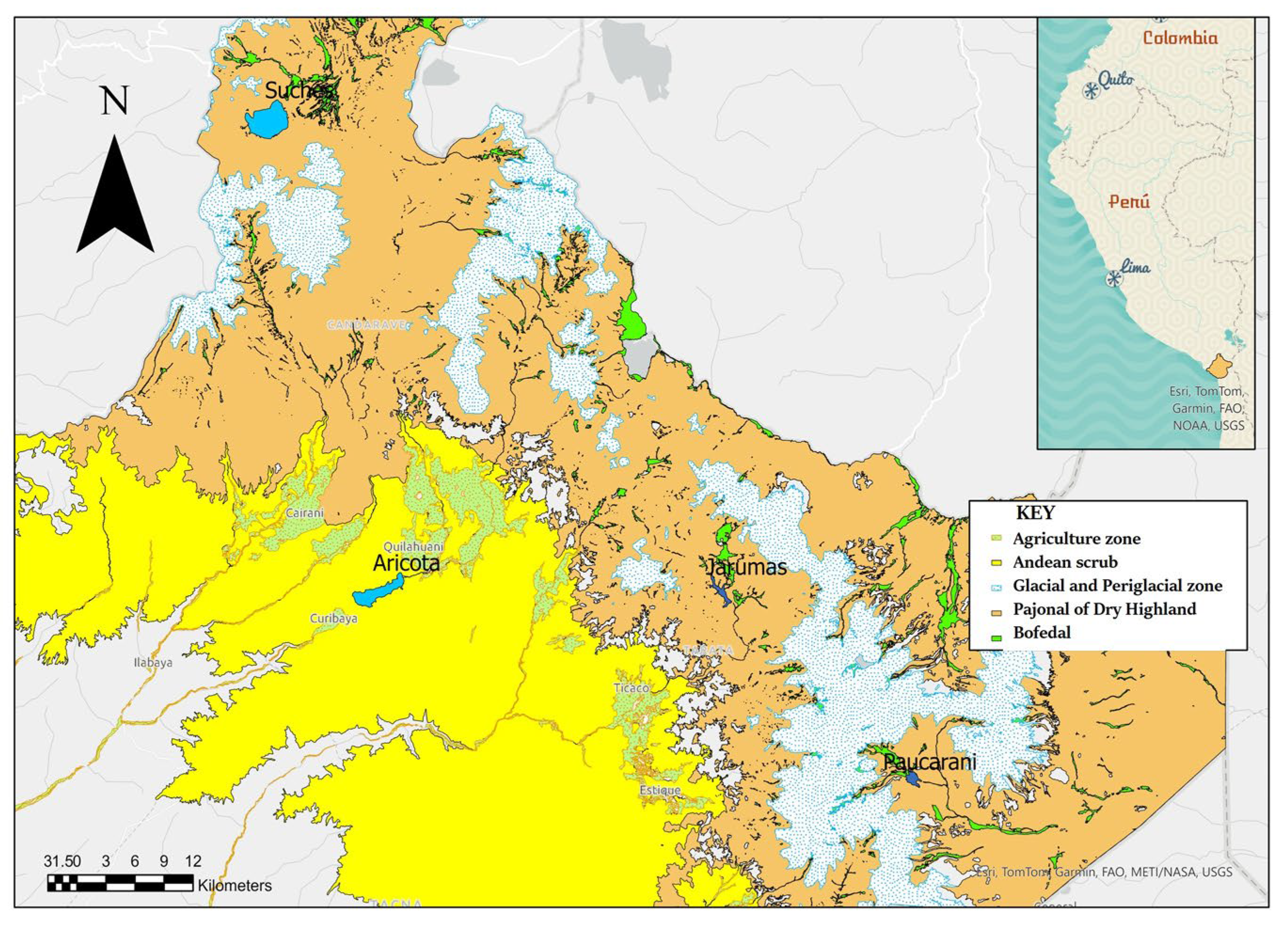
The assessed high Andean system comprises two natural lagoons—Suches (4,460 m asl) and Aricota (2,800 m asl)—and two regulated reservoirs—Jarumas (4,500 m asl) and Paucarani (4,560 m asl)—located on the western slope of the southern Peruvian Andes (Moquegua–Tacna regions). According to Chief Resolution No. 056-2018-ANA, the first three water bodies are classified as Category 4 E1 (aquatic environment conservation), while Paucarani corresponds to Category 1 A2 (supply for human consumption with conventional treatment).
Each lentic body contains fixed monitoring stations (Code: type-name-number) with vertical replication at two depths: surface (~0.3 m) and optical bottom, defined as the depth equal to the Secchi disk transparency value (range 1.2–5 m across systems).
The network includes: Suches (n = 2, cod. LSuch1 and LSuch2), Aricota (n = 3, LAric1, LAric2 and LAric3), Jarumas (n = 2, EJaru1, EJaru2; series 2015–2021 and 2024) and Paucarani (n = 2, EPauc1, EPauc2; series 2015–2017, 2021 and 2024). For spatial–statistical consistency, stations were treated as nested within each water body and all analyses downstream were conducted at the lake×stratum level; geographic coordinates and station metadata are reported in Table 1, and strata were defined a priori as surface (≈0.3 m) and optical bottom (depth=Secchi).
The four water bodies evaluated exhibit distinct anthropogenic pressures. Suches Lagoon, endorheic in nature, receives seasonal flows from small streams that drain wetlands occupied by camelids (alpacas and llamas); although these tributaries meet environmental quality standards (ECA-water, category 4E2), their flows are far below the demands of local mining activities. Furthermore, the lagoon houses aquaculture cages for Oncorhynchus mykiss (rainbow trout) and shows progressive deterioration of the surrounding wetlands. Aricota Lagoon is exploited for hydropower purposes and supports intensive trout production; it receives discharges from the Callazas y Salado River, whose total phosphorus and arsenic exceed the ECA-4E2 limits, generating a local source of contamination. The Jarumas Reservoir, used primarily for agricultural irrigation, also supports trout farming; its main tributary comes from well-preserved wetlands and meets ECA-4E2. The Paucarani Reservoir supplies water for irrigation and public consumption, but its tributary drains wetlands with high concentrations of heavy metals, posing a potential risk to human health. All systems receive their most significant hydrological input during the rainy season (January-March), when peak flow and nutrient loading occur.
Figure 1.
Location of the lagoons and reservoirs assessed on the western slope of southern Peru. The main uses and surrounding ecological units are indicated.
Figure 1.
Location of the lagoons and reservoirs assessed on the western slope of southern Peru. The main uses and surrounding ecological units are indicated.
2.2. Database
A total of 1,846 historical records (2015–2024) were downloaded from the Water Observatory module of the National Water Resources Information System (SNIRH) (https://snirh.ana.gob.pe/onrh/), exclusively selecting official surveys from the National Water Authority (ANA). The years with information were: 2015–2021 and 2024 for Suches, Aricota, and Jarumas I; and 2015, 2016, 2017, 2021, and 2024 for Paucarani. Each record contains the date, sampling depth (surface “S” or bottom “F”), and up to 52 physicochemical and microbiological variables analyzed on-site and in an ISO 17025-accredited laboratory. Data-availability matrices by lake×year guided inclusion criteria: a lake–year was retained when at least one complete campaign (surface and bottom) was available for the core set of variables required by the indices. Decadal analyses used annual means by lake and stratum for 2015–2024; inter-lake comparisons were restricted to years common to all four systems (2015, 2016, 2017, 2021), yielding n = 40 aggregated observations for the comparative tests. All inclusion/exclusion decisions are documented in Supplementary Table S1 and mirrored in the released scripts.
2.3. Pre-Processing and Calculation of Derived Variables
2.3.1. Data Standardization and Quality Control
Data processing was performed in R 4.3.2 [15] under Windows 11 Pro, primarily using the tidyverse, lubridate, janitor, openxlsx, and LakeMetabolizer packages. Full scripts are provided as Supplementary Material S1–S8. Header normalization. Data were transformed to snake_case with janitor::clean_names().
2.3.2. Unit Conversions
Unit conversions were performed selectively according to each index's original formulation. (1) Metals (As, Cd, Cu, Cr, Zn, Pb, Ni, Hg) were converted from mg L⁻¹ to µg L⁻¹ (×1,000) for three indices (HPI, CD, CCME-WQI) to match Peruvian water quality standards (DS 004-2017-MINAM Annex 3), while remaining in mg L⁻¹ for WQIHA following the original formulation [16]. (2) Chlorophyll-a, total phosphorus, and total inorganic nitrogen were converted to µg L⁻¹ for trophic indices (TRIX, TSItsr, OECD) as originally calibrated [17,18,19], but remained in mg L⁻¹ for WQIHA and OWQI. (3) Percent oxygen saturation was calculated using LakeMetabolizer::o2.at.sat.base() [20] for indices requiring saturation metrics. All other parameters retained their analytical units, ensuring consistency with published methodologies and regulatory standards This index-specific approach prevents systematic errors from inappropriate unit transformations and ensures compatibility with regulatory frameworks.
2.3.3. Derived Variables
Turbidity approximation. When direct turbidity measurements were unavailable, nephelometric turbidity (NTU) was approximated from total suspended solids (TSS, mg L⁻¹) using the linear relationship NTU = 1.5×TSS + 2.0 (Eq. 01). This approach is justified by: (1) well-established TSS-turbidity correlations (r = 0.77–0.96) across diverse aquatic systems [21]; with relationships particularly robust in semi-arid reservoirs and tropical systems [22]; (2) our TSS range (0.5–37 mg L⁻¹, n=145 measurements) is well below thresholds where approximations degrade (>800 mg/L; [23), yielding turbidity estimates (2.75–57.5 NTU) representing only 9.6% of the reliable measurement range (<600 NTU); and (3) turbidity's limited contribution (~2–4%) to the final WQIHA score ensures minimal impact on classifications (estimated uncertainty: ±0.5–1.0 WQIHA units vs. 20-unit category widths).
While TSS-turbidity relationships are inherently site-specific [24], the conservative concentration range, predominantly mineral particle composition typical of oligotrophic high-altitude systems, and constrained influence on final indices support the approximation's appropriateness. Future monitoring should include paired TSS-turbidity measurements for site-specific validation.
Total inorganic nitrogen (TN = [NH₄-N] + [NO₂-N] + [NO₃-N]) was calculated additively.
2.3.4. Record Filtering and Missing Data Handling
Record filtering. For each index, only samples with the minimum required parameters were retained; the absence of auxiliary variables was authorized as long as the algorithm did not alter the original index structure (e.g., TRIX without NO₂ if NO₃ and NH₄ were present).
Censored values. Values below detection limits (< LOD) were imputed as LOD/2 [17], applied only when censoring per variable was <10%, consistent with recent guidance for environmental datasets.
Weight renormalization. For indices calculated with incomplete parameter sets, weights were renormalized to sum to 1.0, maintaining original relative proportions. This approach is consistent with CCME [25) recommendations and allows index calculation with missing data while maintaining interpretability.
WQIHA parameter coverage. WQIHA was calculated with 17 of the 20 standard parameters, representing 85% coverage. Missing parameters (copper, total dissolved solids, oils and greases) were unavailable in the historical monitoring program. Sub-index weights were renormalized to sum to 1.0, maintaining original relative proportions among available parameters, a procedure validated in systems with limited data.
2.4. Water Quality Indices
Three complementary sets of indices characterized water quality from multiple perspectives: trophic state, integrated physicochemical condition, and metal contamination.
2.4.1. Trophic State Indices
Biological productivity was assessed using three complementary indices. The Trophic State Index for tropical/subtropical reservoirs (TSItsr) estimates trophic conditions from two core variables—chlorophyll-a and total phosphorus—using empirical equations specifically calibrated for warm-climate lentic systems (Equation 1). The Trophic Index (TRIX) integrates six parameters to provide a multidimensional assessment: chlorophyll-a, oxygen deficit (calculated as percent saturation deficit), dissolved inorganic nitrogen (DIN = NH₄-N + NO₃-N + NO₂-N), total phosphorus, temperature, and salinity (Equation 2). The OECD classification scheme assigns categorical trophic states—oligotrophic, mesotrophic, eutrophic, or hypereutrophic—based on annual means of three primary indicators: chlorophyll-a, total phosphorus, and Secchi depth transparency, complemented by additional metrics where available.
2.4.2. Integrated Water Quality Indices
Three multimetric indices provided comprehensive assessments by integrating multiple physicochemical parameters into single quality scores. The Water Quality Index for High Andean systems (WQIHA; [16] combines three sub-indices with original weights: physicochemical parameters (SIPC), heavy metals (SIHM), and organic matter indicators (SIOM). This region-specific formulation was developed for high-altitude Andean aquatic systems and employs weighted aggregation to produce a 0–100 scale (Equation 3). The Oregon Water Quality Index (OWQI; [26] calculates the geometric mean of six: temperature, dissolved oxygen, biochemical oxygen demand, pH, total solids, total phosphorus, nitrates, and ammonia (Equation 4). The Canadian Council of Ministers of the Environment Water Quality Index (CCME-WQI; [25] combines three factors: scope (F₁, proportion of variables failing to meet objectives), frequency (F₂, proportion of individual tests failing), and amplitude (F₃, degree by which failed tests deviate from objectives). This study employed Peruvian water quality standards for Category 4-E1 (DS 004-2017-MINAM) as reference objectives, adopting the "unbiased" calculation variant that equally weights the three factors (Equation 5).
2.4.3. Metal Contamination Indices
Two indices quantified heavy metal contamination using different conceptual approaches. The Heavy Metal Pollution Index (HPI; [27] employs inverse-standard weights (Wᵢ = 1/Sᵢ) to emphasize highly regulated metals, where Wᵢ is the weight for metal i and Sᵢ is the regulatory standard. This weighting scheme assigns greater importance to metals with stricter regulatory limits, producing a dimensionless pollution score (Equation 6). The Contamination Degree (CD; [28) calculates an additive pollution measure by summing individual contamination factors (CFᵢ = Cᵢ/Sᵢ) across all metals, where Cᵢ is the measured concentration and Sᵢ is the reference standard. This approach provides a cumulative assessment of multi-metal contamination (Equation 7). Both indices employed Peruvian water quality standards for Category 4-E1 (DS 004-2017-MINAM Annex 3) as reference values, with concentrations expressed in µg L⁻¹. Iron and manganese were excluded from calculations because these elements lack established regulatory limits in Category 4-E1, preventing standardization of their contamination factors.
Sample sizes varied by index based on parameter availability from a common pool of 145 water quality observations collected across all systems and sampling events. Three indices achieved complete coverage (n = 145): HPI and CD because all required metals were systematically measured, and OWQI because its six physicochemical parameters were consistently available. Indices requiring chlorophyll-a—a parameter measured in 63.4% of sampling events—exhibited reduced sample sizes: TSItsr (n = 92, requiring 2 parameters), CCME-WQI (n = 92, requiring 15 parameters with selective missing data), WQIHA (n = 86, requiring 17–20 parameters with weight renormalization), and TRIX (n = 80, requiring 6 simultaneously measured parameters). The OECD classification had the smallest sample size (n = 47) due to the additional requirement of Secchi depth transparency measurements, available in only 51% of events. These varying sample sizes reflect operational constraints inherent to multi-annual monitoring programs in remote high-altitude systems and do not compromise the validity of index-specific assessments, as each index was calculated using the maximum available data for its particular parameter requirements.
2.5. Statistical Analyses
After calculating all water quality indices, a comprehensive statistical framework was applied to characterize spatiotemporal patterns, identify environmental drivers, and classify lake typologies.
2.5.1. Data Aggregation and Reconciliation
For each index, annual means were calculated by lake and stratum (surface vs. bottom), with standard deviations computed to quantify within-year variability (Supplementary Code S1–S8). Uneven temporal coverage across lakes was reconciled through two strategies: (i) restricting inter-lake comparisons to years common to all systems (2015, 2016, 2017, 2021), yielding n = 40 aggregated observations; and (ii) for hierarchical clustering, retaining only lake×year×stratum cases with complete seven-index vectors to avoid bias from missing data. This pipeline—1,846 measurements → annual lake×stratum means → complete-case multimetric vectors—ensures comparability while maintaining statistical rigor.
2.5.2. Temporal Trend Analysis
Monotonic temporal trends were evaluated using the nonparametric Mann-Kendall test coupled with the Theil-Sen slope estimator (α = 0.05). This rank-based combination was preferred over ordinary least squares for three reasons: (i) several index series exhibited non-normal distributions (Shapiro-Wilk tests), violating OLS assumptions; (ii) outliers were present in HPI and CD indices, which disproportionately influence least-squares but not rank-based methods; and (iii) short time series (n ≈ 10 years) favor Mann-Kendall, which maintains adequate power while OLS suffers from limited degrees of freedom. The Theil-Sen estimator provides robust trend magnitude estimates insensitive to outliers [29].
2.5.3. Spatial Heterogeneity Assessment
Spatial differences among lake systems were assessed using Kruskal-Wallis tests, a nonparametric alternative to ANOVA that does not assume normality. When significant heterogeneity was detected (p < 0.05), pairwise comparisons used Dunn's post-hoc test with Bonferroni correction to control family-wise type I error rates below α = 0.05.
2.5.4. Multivariate Ordination
Environmental drivers were identified using distance-based redundancy analysis (db-RDA) implemented via vegan::capscale, fitting Euclidean distances on Z-standardized indices and constraining by lake (factor), year (numeric), and hydrological period (wet/dry). This approach allows direct ordination of multimetric matrices without assuming linear relationships between indices and predictors. Model significance was assessed through 999 Monte Carlo permutations (vegan::anova.cca), and variance partitioning used adjusted R² to provide unbiased estimates comparable across models. Due to limited chlorophyll-a availability prior to 2018, the db-RDA with complete seven-index datasets (n=28) was restricted to 2018-2024 dry-season samples. Hydrological period was consequently excluded from the model.
2.5.5. Hierarchical Clustering
Lake ecosystems were classified using Ward's agglomerative hierarchical clustering on Euclidean distances of Z-standardized indices, minimizing within-cluster variance to produce compact groups. The optimal number of clusters (k) was determined through triangulation of three criteria: (i) average silhouette width (values >0.5 indicate strong structure); (ii) elbow method on within-cluster sum of squares; and (iii) gap statistic with 500 bootstrap replicates. All three criteria converged on k = 4 (Supplementary Material Code S8–S12).
2.5.6. Index Intercorrelations
Relationships among seven continuous indices (TSItsr, TRIX, OWQI, WQIHA, CCME-WQI, HPI, CD) were quantified using Pearson correlations from annual lake×stratum means (2015–2024) with pairwise complete observations. The OECD trophic classification was excluded from correlation analysis due to its categorical nature (oligotrophic, mesotrophic, eutrophic, hypereutrophic), which is incompatible with parametric correlation methods designed for continuous variables. Distributional assumptions were verified via Shapiro-Wilk tests and Q-Q plots. Given 21 pairwise correlations, p-values were Bonferroni-adjusted (α_adjusted = 0.05/21 = 0.0024) to control family-wise error rates. Correlation patterns were interpreted considering both statistical significance and effect size. Tests used R 4.3.2 (stats::cor.test) with exact two-sided confidence intervals.
2.6. Computational Environment and Reproducibility
All analyses were executed in R 4.3.2 [30] on Windows 11 Pro. Key packages: tidyverse 2.0.0, lubridate 1.9.3, janitor 2.2.0, openxlsx 4.2.5.2, vegan 2.6-6, cluster 2.1.6, factoextra 1.0.7, and Kendall 2.2.1.
Reproducibility was ensured through three mechanisms: (i) seeding stochastic procedures with set.seed(12345) for identical results across runs; (ii) exporting complete session information via sessionInfo(); and (iii) fully scripting all transformations and quality controls (Supplementary Code S1–S8) with no manual manipulation.
Data and code availability. All R scripts, intermediate data, and outputs are publicly available in the Zenodo repository (DOI: 10.5281/zenodo.16401603), including annotated code, input data (.xlsx and .csv formats), and computed indices.
2.7. Artificial Intelligence Disclosure
During R code development, ChatGPT (GPT-o3, OpenAI, May 2025) assisted with refactoring non-vectorized code for efficiency and clarifying vegan and cluster syntax. All AI-generated suggestions were independently validated through package documentation, test cases, and comparison with published methods. All analytical decisions—statistical methods, significance thresholds, transformations, and interpretation—were author-driven and independent of AI assistance [31].
3. Results
3.1. Trophic State Classification
3.1.1. TSItsr-Based Assessment
TSItsr values across the four lake systems ranged from 48.3 to 57.8 (mean ± SD: 52.8 ± 3.4), indicating predominantly mesotrophic conditions during 2018–2024. Aricota exhibited the highest average TSItsr (55.4 ± 2.0), followed by Suches (52.8 ± 3.1) and Jarumas (50.9 ± 3.2), while Paucarani showed the lowest values (48.6 ± 0.5), approaching the mesotrophic–oligotrophic boundary (Table 1). Within-lake variability was moderate, with coefficients of variation ranging from 1% (Paucarani) to 6% (Jarumas), reflecting relatively stable trophic conditions over the study period despite interannual fluctuations in chlorophyll-a concentrations.
3.1.2. OECD Classification
According to OECD criteria based on chlorophyll-a and total phosphorus thresholds, three lakes were classified as mesotrophic (Aricota, Jarumas, Suches) and one as oligotrophic (Paucarani). No system reached eutrophic status (TSItsr > 59) during the monitoring period, though Aricota approached this threshold in 2018 (TSItsr = 57.8). The oligotrophic classification of Paucarani appears paradoxical given its elevated metal concentrations (Section 3.3), suggesting that geogenic contamination may suppress phytoplankton productivity despite nutrient availability—a pattern documented in other metal-impacted Andean lakes.

Table 2.
Trophic state classification of high Andean lakes based on TSItsr and OECD criteria (2018–2024, n = 28 complete cases).
Table 2.
Trophic state classification of high Andean lakes based on TSItsr and OECD criteria (2018–2024, n = 28 complete cases).
| Lake | TSItsr Range | Mean ± SD | OECD Class | n |
| Aricota | 52.0–57.8 | 55.4 ± 2.0 | Mesotrophic | 10 |
| Suches | 48.8–55.0 | 52.8 ± 3.1 | Mesotrophic | 6 |
| Jarumas | 48.3–55.8 | 50.9 ± 3.2 | Mesotrophic | 10 |
| Paucarani | 48.3–49.0 | 48.6 ± 0.5 | Oligotrophic | 2 |
| Overall | 48.3–57.8 | 52.8 ± 3.4 | — | 28 |
Note. TSItsr calculated using Carlson's modified index for surface waters. OECD classification: oligotrophic (TSItsr < 50), mesotrophic [50–59), eutrophic (> 59). n = number of complete lake-stratum-year observations with chlorophyll-a data (2018–2024).
3.2. Temporal Stability: Mann–Kendall and Theil–Sen
Having established baseline trophic conditions, we next examined whether systematic temporal changes occurred across water quality indices over the decade-long monitoring period.
3.2.1. General Summary of Significance
High Andean lakes exhibited remarkable temporal stability across water quality indices. Mann–Kendall tests on 56 lagoon–stratum × index combinations (8 configurations × 7 multimetric indices) revealed no significant monotonic trends in 96.4% of cases (54/56, p > 0.05), indicating persistent water quality conditions over 2015–2024 (Figure 2a). Only two exceptions showed statistically significant declines: CCME-WQI in both strata of Jarumas Reservoir (surface: τ = –2.35, p = 0.019; bottom: τ = –2.35, p = 0.019)
For transparency, effective sample sizes varied by system: Suches, Aricota, and Jarumas had 8 years each (2015–2021, 2024; n = 8), while Paucarani had 5 years (2015–2017, 2021, 2024; n = 5). Trend tests were run with the effective years available for each lagoon–stratum combination. The phrase "2015–2024 (10 nominal years)" is used only as a temporal reference window, acknowledging gaps in 2022–2023 due to pandemic-related sampling constraints.
Figure 2a.
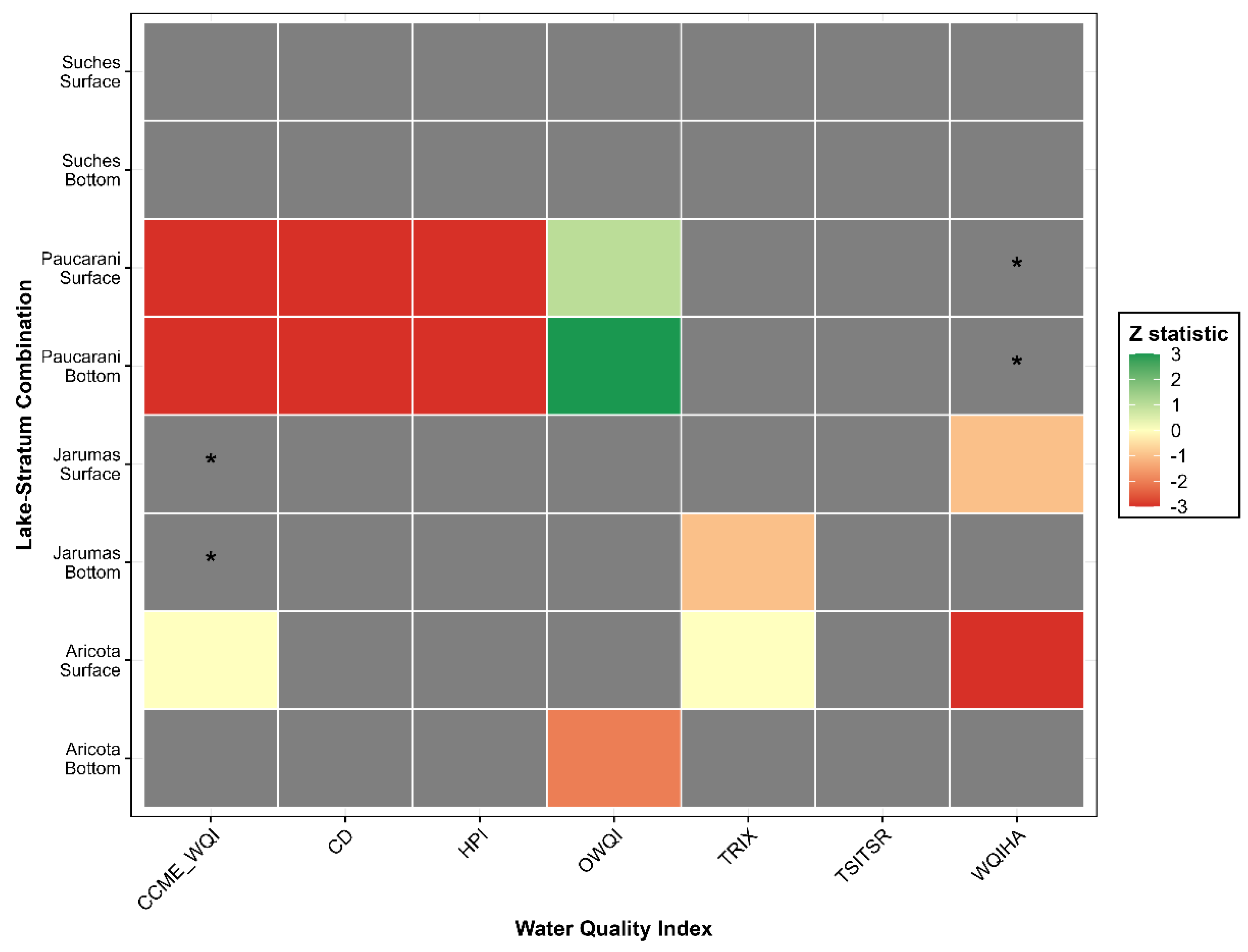
Mann-Kendall trend analysis of water quality indices across high Andean lakes (2015–2024). Heatmap shows Z statistics for 56 lagoon-stratum × index combinations. Green indicates positive trends, red indicates negative trends, yellow indicates near-zero trends. Asterisks (*) denote statistical significance at p < 0.05. Only 4 of 56 cases (7.1%) showed significant trends (Jarumas CCME-WQI and Paucarani WQIHA, both strata), indicating overall temporal stability across the study period. Note: Complete outputs (Kendall's S, Z statistic, p-value, and Theil–Sen slope) are available at Zenodo (DOI: 10.5281/zenodo.16401603).
Figure 2a.
Mann-Kendall trend analysis of water quality indices across high Andean lakes (2015–2024). Heatmap shows Z statistics for 56 lagoon-stratum × index combinations. Green indicates positive trends, red indicates negative trends, yellow indicates near-zero trends. Asterisks (*) denote statistical significance at p < 0.05. Only 4 of 56 cases (7.1%) showed significant trends (Jarumas CCME-WQI and Paucarani WQIHA, both strata), indicating overall temporal stability across the study period. Note: Complete outputs (Kendall's S, Z statistic, p-value, and Theil–Sen slope) are available at Zenodo (DOI: 10.5281/zenodo.16401603).
3.2.2. Directionality of Trend Signals
Although most trends were statistically non-significant, their directionality was not evenly distributed. Negative trends (τ < 0) dominated 71.4% of cases (40/56), concentrating in Jarumas and Aricota—particularly for TSItsr and WQIHA—suggesting subtle but widespread water quality deterioration pressures. In contrast, positive trends (τ > 0) comprised only 14.3% (8/56), with Suches exhibiting the strongest improvement signals (e.g., OWQI, Z = +1.36). The remaining 14.3% of series (8/56) showed near-zero trend statistics (|τ| ≤ 0.5), consistent with complete temporal stability. This asymmetry toward negative trends, though largely non-significant individually, may reflect cumulative anthropogenic pressures (mining legacy, agricultural runoff) that are not yet manifesting as statistically detectable changes at the decadal scale.
3.2.3. Magnitude of Change (Theil–Sen)
Theil–Sen slopes confirmed the slow rate of change across all indices. For indices expressed on 0–100 scales (CCME-WQI, OWQI), all slopes were < 1.5 units·year⁻¹, representing < 15% change per decade—well below operational thresholds for water quality reclassification. The steepest decline occurred in WQIHA at Paucarani (–16.0 units·year⁻¹ at surface, –14.6 at bottom), driven primarily by increasing turbidity and metal loadings from geogenic sources. Conversely, the strongest improvement was observed in OWQI at Suches (+1.8 units·year⁻¹), reflecting stable oligotrophic conditions and minimal anthropogenic impacts in this remote, endorheic system.
Decadal projections based on observed slopes indicate that even the largest absolute changes (e.g., CCME-WQI decline at Jarumas: –1.4 units·year⁻¹ × 10 years = –14 units) would not cross qualitative class boundaries. For instance, Jarumas CCME-WQI ranged 39–52 during 2015–2024; a 10-year extrapolation (2024 value: 42 → 2034 projection: 28) would remain within the "Marginal" category [20,21,22,23,24,25,26,27,28,29,30,31,32,33,34,35,36,37,38,39,40,41,42,43,44], avoiding reclassification to "Poor" (< 20). This robustness reflects the conservative design of multimetric indices, which buffer against short-term fluctuations while remaining sensitive to sustained, directional changes.
Table S3. Theil–Sen slopes (unit·year⁻¹) for all lagoon–stratum × index combinations. Available at Zenodo (DOI: 10.5281/zenodo.16401603).
3.3. Spatial Heterogeneity Among Lake Systems
In contrast to temporal stability, pronounced spatial differences emerged among the four lake systems, reflecting divergent environmental pressures and limnological characteristics.
3.3.1. Global Significance Tests
Kruskal–Wallis tests detected significant inter-lake differences for four of seven indices (n = 40 observations per index: 4 lakes × 2 strata × 5 common years). CCME-WQI (H₃ = 29.1, p < 0.001, ε² = 0.73) and CD (H₃ = 26.6, p < 0.001, ε² = 0.66)) showed the strongest spatial heterogeneity, with very large effect sizes indicating that lake identity explains > 70% of variance in these indices. HPI (H₃ = 18.1, p < 0.001, ε² = 0.42) and WQIHA (H₃ = 12.8, p = 0.005, ε² = 0.28) also differed significantly, though with moderate-to-large effects. In contrast, OWQI (H₃ = 5.6, p = 0.135), TSItsr (H₃ = 5.9, p = 0.116), and TRIX (H₃ = 4.6, p = 0.102) showed no significant differences, suggesting that trophic state metrics are more homogeneous across systems than contamination-sensitive indices.
Table S4. Global Kruskal–Wallis test statistics for inter-lake differences (2015–2024, n = 40). Effect size ε² = (H − k + 1)/(N − k), where k = 4 lakes and N = 40. Magnitude criteria: ε² < 0.08 = small, 0.08–0.26 = moderate, ≥ 0.26 = large. Available at Zenodo (DOI: 10.5281/zenodo.16401603).
3.3.2. Pairwise Contrasts (Dunn–Bonferroni)
Post-hoc Dunn–Bonferroni tests revealed consistent, significant differences for specific lake pairs (α = 0.05, Table S5):
- (1)
- Aricota vs. Suches: Differed in CCME-WQI (p < 0.001, Δmedian = –37 units), CD (p = 0.012, Δ = +2.2 μg L⁻¹), and WQIHA (p = 0.015, Δ = –14 units), with Aricota consistently exhibiting poorer water quality across multiple metrics.
- (2)
- Paucarani vs. Suches: Showed extreme differences in CD (p < 0.001, Δ = +23 μg L⁻¹) and HPI (p < 0.001, Δ = +179 units), reflecting Paucarani's geogenic metal contamination from volcanic-hydrothermal sources.
- (3)
- Jarumas vs. Paucarani: Differed in CD (p = 0.0002, Δ = –23 μg L⁻¹) and HPI (p = 0.0014, Δ = –176 units), underscoring the uniqueness of Paucarani's geochemical signature.
- (4)
- Aricota vs. Jarumas: Showed smaller but significant differences in CCME-WQI (p = 0.006, Δ = –19 units) and CD (p = 0.039, Δ = +2 μg L⁻¹).
- (5)
- Jarumas vs. Suches: No significant differences in any index, suggesting comparable water quality despite different anthropogenic pressures (agricultural runoff in Jarumas vs. minimal impacts in Suches).
Effect sizes (partial ε²) ranged from 0.11 (small: WQIHA, Aricota–Suches) to 0.41 (very large: CCME-WQI, Aricota–Suches), indicating that some contrasts represent ecologically meaningful differences while others are statistically detectable but modest in magnitude.
Table S4. Dunn–Bonferroni pairwise comparisons (2015–2024). Median differences (Δ), z statistic, adjusted p-value, and partial effect size (ε²_parc = z²/(N − 1)). Only significant contrasts (p < 0.05) reported. Available at Zenodo (DOI: 10.5281/zenodo.16401603).
3.3.3. Dispersion and Rank Ordering
Boxplot distributions (Figure 2c) visualize median rankings and interquartile variability:
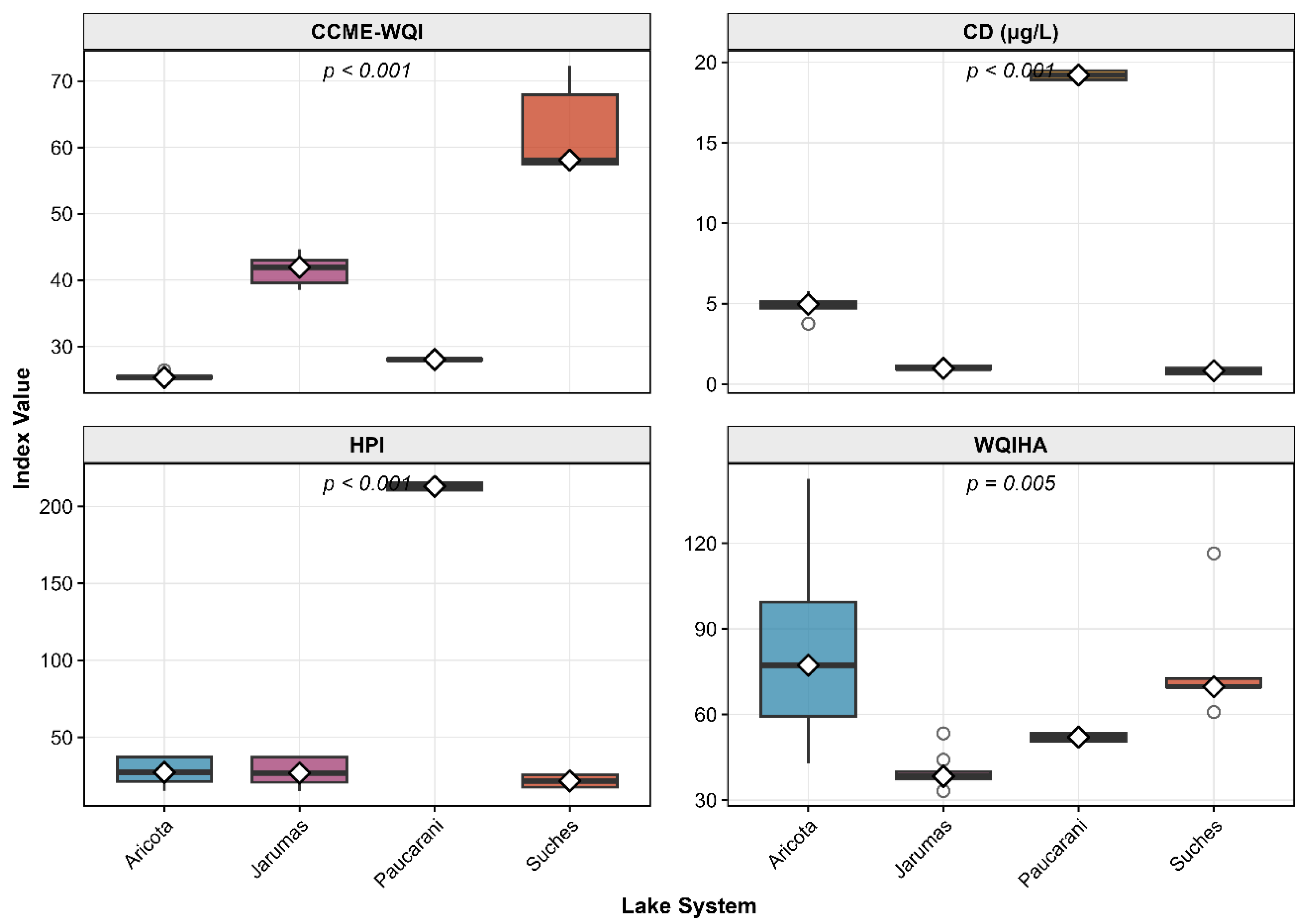
CCME-WQI: Ascending order Aricota < Paucarani ≈ Jarumas < Suches, consistent with anthropogenic pressure gradients (legacy mining in Aricota vs. pristine conditions in Suches).
CD: Minimum dispersion in Jarumas (IQR = 0.3 μg L⁻¹), maximum in Paucarani (IQR = 2.4 μg L⁻¹), reflecting Paucarani's temporally variable geogenic inputs.
HPI: Paucarani clearly separated from other systems (median ≈ 214 vs. 23–50), driven by elevated As, Pb, and Cd concentrations.
OWQI: Wide overlap among all lakes, consistent with the non-significant global test—indicating that dissolved oxygen regimes are relatively uniform across systems despite differences in trophic state and contamination.
Figure 2c.
Spatial heterogeneity in water quality indices among high Andean lakes (2015–2024, n = 10 observations per lake). Boxplots show median (white diamonds), interquartile range (boxes), and outliers (white circles) for four indices that exhibited significant inter-lake differences: (A) CCME-WQI (Canadian Council of Ministers of the Environment Water Quality Index), (B) CD (Contamination Degree in μg L⁻¹), (C) HPI (Heavy Metal Pollution Index), and (D) WQIHA (Water Quality Index for High Andean systems). Kruskal-Wallis p-values shown in each panel. Paucarani shows distinctively elevated metal contamination (HPI, CD) while maintaining relatively low CCME-WQI, reflecting geogenic metal inputs that suppress trophic indicators.
3.4. Environmental Drivers of Water Quality Variation
To identify the underlying mechanisms governing spatial and temporal patterns, we applied multivariate ordination techniques to the complete seven-index dataset.
3.4.1. Inter-Index Correlations
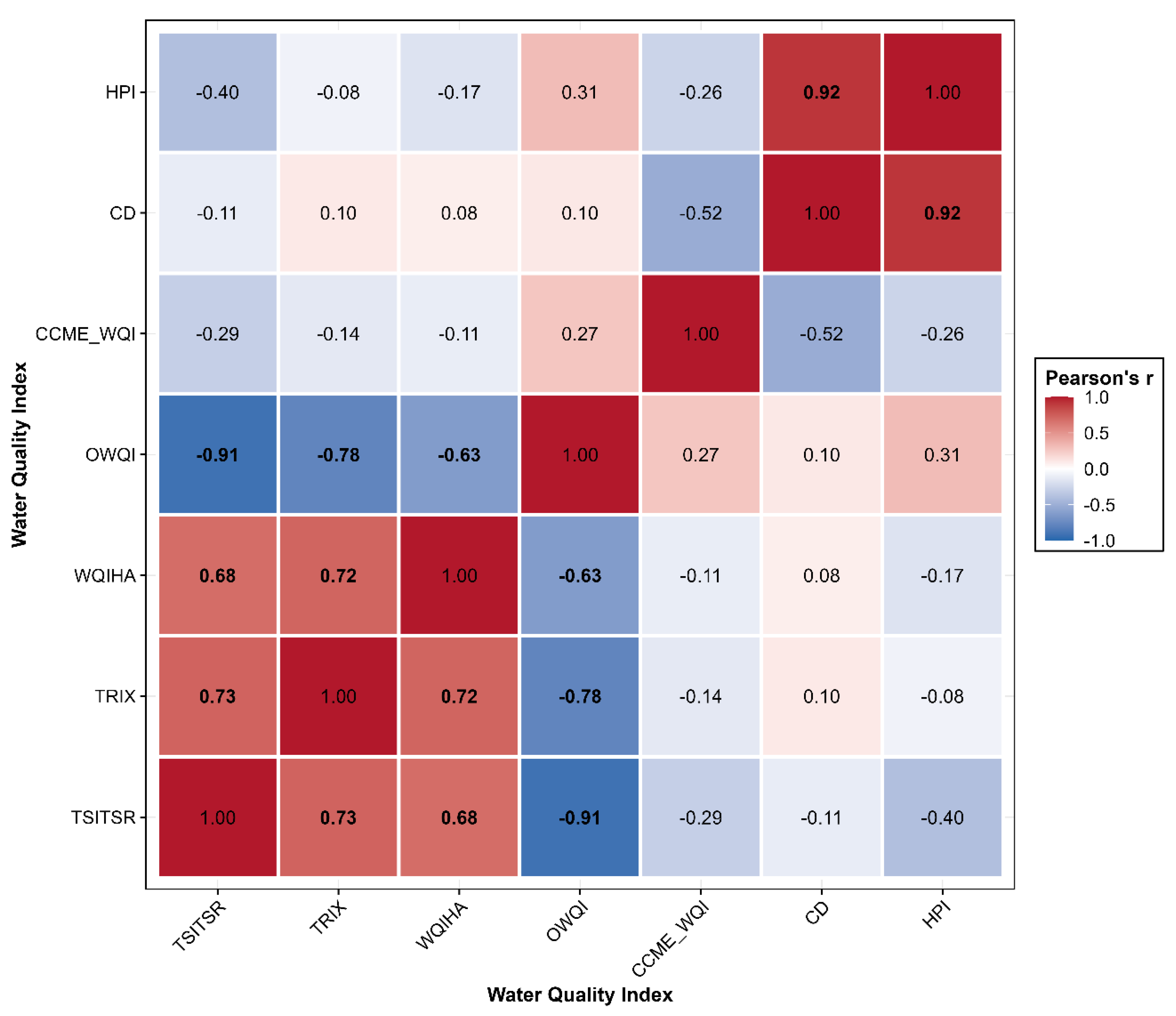
Pearson correlation analysis (Figure 3a, n = 40 annual means, Bonferroni-adjusted for 21 comparisons) revealed six significant pairings (|r| ≥ 0.53, p < 0.05):
CD–HPI (r = 0.92): Very strong positive correlation, indicating that metal contamination drives heavy metal pollution index variation.
OWQI–TSItsr (r = –0.91): Strong negative correlation, confirming that oxygen conditions deteriorate with increasing trophic state.
TSItsr–WQIHA (r = 0.68) and TRIX–WQIHA (r = 0.72): Moderate positive correlations, linking trophic indicators to habitat quality degradation.
CCME-WQI–WQIHA (r = –0.59): Moderate negative correlation, reflecting trade-offs between overall water quality and habitat-specific metrics.
OWQI–TRIX (r = –0.53): Moderate negative correlation, consistent with oxygen depletion under elevated nutrient conditions.
These associations suggest that water quality indices, though conceptually distinct, share underlying drivers related to trophic state (OWQI, TSItsr, TRIX, WQIHA) and contamination (CD, HPI), while CCME-WQI integrates multiple stressors. Moderate-strength correlations (0.40–0.53) that did not survive Bonferroni adjustment—such as TSItsr–TRIX (r = 0.43)—indicate partial redundancy but justify retaining all seven indices for comprehensive assessment.
Figure 3.
a. Pearson correlation matrix for seven water quality indices (n = 28 complete cases, 2018–2024). Color gradient indicates correlation strength: blue (negative), white (zero), red (positive). Bold values indicate correlations significant after Bonferroni adjustment (|r| ≥ 0.53, p < 0.002 for 21 comparisons). Six significant pairings emerged: CD–HPI (r = 0.92, metal contamination axis), OWQI–TSItsr (r = –0.91, oxygen-trophic state trade-off), TSItsr–WQIHA (r = 0.68), TRIX–WQIHA (r = 0.72), CCME-WQI–WQIHA (r = –0.59), and OWQI–TRIX (r = –0.53). Moderate correlations suggest indices capture distinct but partially overlapping water quality dimensions.
3.4.2. Distance-Based Redundancy Analysis (db-RDA)
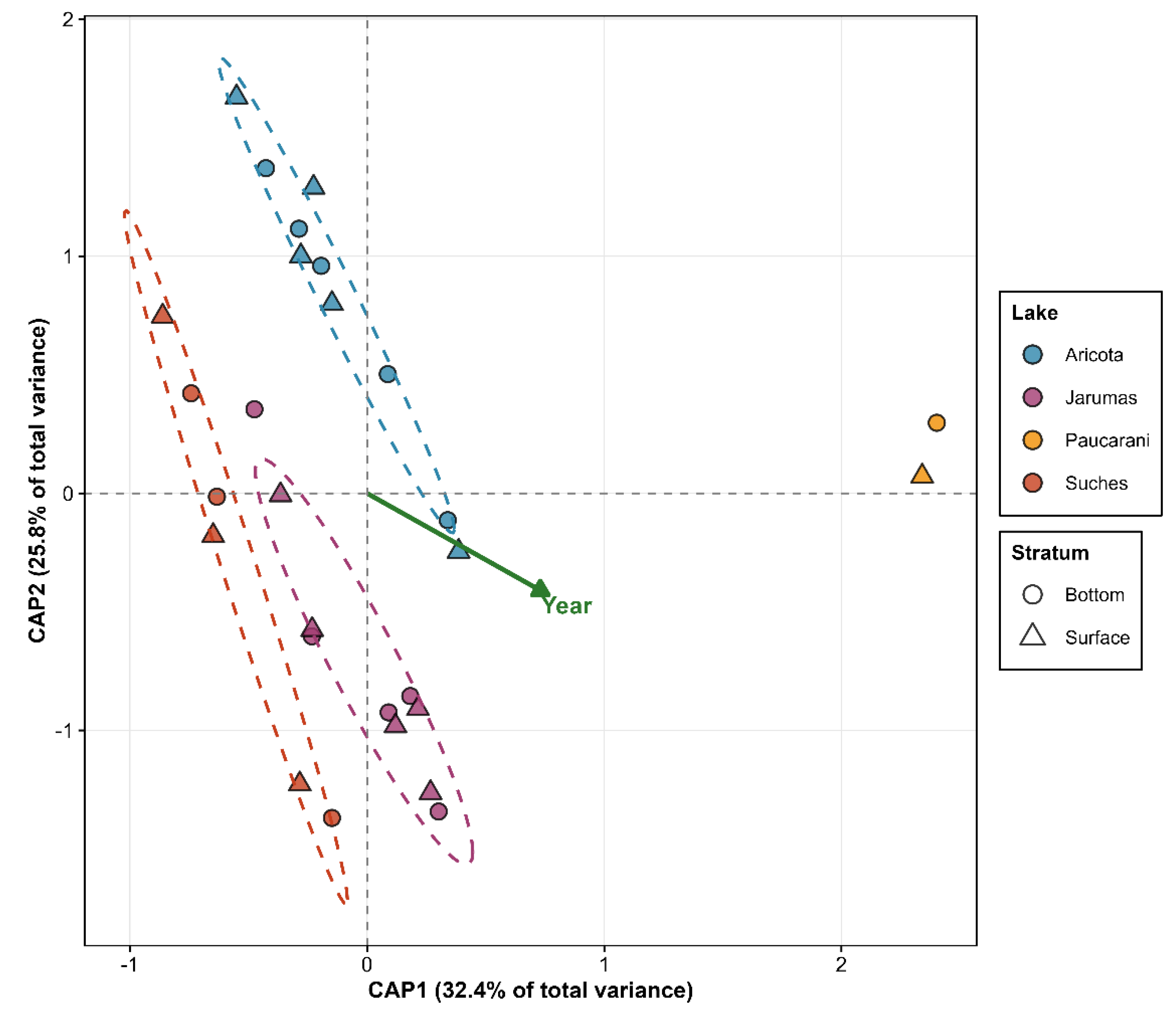
Distance-based redundancy analysis on Euclidean distances of Z-standardized indices (n = 28 complete cases from 2018–2024) was statistically significant (p = 0.001), with an adjusted R² of 0.621 (62.1% of total variance explained). The first two constrained axes accounted for 32.4% (CAP1) and 25.8% (CAP2) of variation, respectively. Permutational tests (999 permutations, set.seed = 12345) identified lake identity as the dominant driver (F₃,₂₃ = 15.15, p = 0.001), explaining approximately 45% of constrained variance, followed by year (F₁,₂₃ = 2.76, p = 0.050), contributing approximately 8%. No lake × stratum interaction reached significance (p > 0.10), reinforcing the vertical homogeneity observed in univariate analyses (Section 3.3).
Hydrological period effects (wet vs. dry season) could not be evaluated because all complete-case observations corresponded to dry-season samples—a consequence of chlorophyll-a measurement availability being restricted to 2018–2024 dry-season campaigns. Future studies incorporating wet-season chlorophyll-a data would enable seasonal driver assessment, though prior work in tropical Andean lakes suggests that seasonal effects are typically smaller than spatial differences at high altitudes (> 3800 m a.s.l.) where thermal stratification is weak or absent.
Figure 3.
b. Distance-based redundancy analysis (db-RDA) biplot showing environmental drivers of water quality variation (n = 28 complete cases, 2018–2024). Ordination based on Euclidean distances of Z-standardized indices. Model explained 32.4% of total variance (adjusted R² = 0.621, p = 0.001, 999 permutations). First two constrained axes account for 32.4% (CAP1) and 25.8% (CAP2) of variation. Symbols represent samples colored by lake (blue = Aricota, purple = Jarumas, orange = Paucarani, red = Suches) and shaped by stratum (triangles = surface, circles = bottom). Dashed ellipses show 68% confidence intervals per lake. Green arrow indicates year gradient (continuous variable). Lake identity was the dominant driver (F₃,₂₃ = 15.15, p = 0.001, ~45% of constrained variance), followed by year (F₁,₂₃ = 2.76, p = 0.050, ~8%). Hydrological period could not be evaluated as all observations were dry-season samples. CAP1 primarily reflects temporal improvement (recent years right, early years left), while CAP2 separates contamination gradient (Paucarani high, Suches low). Note: Sample coordinates, index loadings, and complete permutational p-values are available in supplementary files Scores_Samples_dbRDA.csv, Scores_Indices_dbRDA.csv, and Scores_Variables_dbRDA.csv (Zenodo: DOI: 10.5281/zenodo.16401603).
3.4.3. Ordination Gradients and Ecological Interpretation
CAP1 (32.4% of variation) primarily reflected a temporal gradient: positive scores aligned with recent years (2021–2024) and higher OWQI and CCME-WQI, whereas negative scores corresponded to 2018–2019 with elevated TSItsr and TRIX. This axis captures gradual water quality improvement across systems, potentially linked to reduced mining inputs (Aricota) and stabilization of agricultural practices (Jarumas).
CAP2 (25.8% of variation) separated systems spatially along a contamination axis: Paucarani (upper-right quadrant) exhibited extreme positive CAP2 scores due to elevated HPI and CD from geogenic metal sources, while Suches (lower-left quadrant) showed negative CAP2 scores reflecting pristine, low-metal conditions. Jarumas and Aricota occupied intermediate positions, with Jarumas skewing toward Suches (moderate agricultural impacts) and Aricota toward Paucarani (legacy mining contamination), consistent with pairwise contrast results (Section 3.3.2).
The lack of stratum effects (p > 0.10 for surface vs. bottom interaction) indicates that vertical stratification is weak in these shallow (< 15 m), wind-exposed high-altitude lakes, allowing for relatively uniform water quality throughout the water column—a pattern commonly observed in polymictic tropical mountain lakes.
3.5. Functional Typology: Ward Hierarchical Clustering
To synthesize spatiotemporal patterns into ecologically interpretable groups, we applied hierarchical clustering to the complete seven-index profiles.
3.5.1. Partition Robustness and Optimal k
Ward's hierarchical clustering on Euclidean distances of Z-standardized indices identified four functional lake groups from n = 28 complete-case observations (4 lakes × 2 strata × years 2018–2024). The optimal partition at k = 4 emerged through triangulation of multiple validation criteria: average silhouette width (0.43), peak gap statistic (0.49), and maximum Calinski-Harabasz index (29.1) (Table S5). Although k = 3 exhibited marginally superior silhouette performance (0.48 vs. 0.43), the four-cluster solution was ultimately selected because it (i) maximized convergence across two of three quantitative metrics, and (ii) preserved ecologically interpretable subdivisions that would otherwise be conflated. Specifically, k = 4 successfully disentangled Aricota's persistent mesotrophic-contaminated signature (Cluster 1) from the temporally improving mixed assemblage of Jarumas–Suches–Aricota samples (Cluster 2)—a distinction critical for targeted management interventions yet obscured under the k = 3 configuration.
Figure 3.
c. Ward hierarchical clustering dendrogram identifying functional typologies (n = 28 complete cases, 2018–2024). Clustering based on Euclidean distances of Z-standardized seven-index profiles. Vertical axis shows Ward's D² linkage distance; horizontal axis shows individual observations (lagoon_stratum_year). Red dashed line indicates optimal cutoff at k = 4 clusters, selected based on maximum silhouette width (0.46), gap statistic (0.49), and Calinski-Harabasz index (29.1). Four distinct functional groups emerged: Cluster 1 (blue, n = 8) encompasses all Aricota observations representing persistent mesotrophy with moderate contamination; Cluster 2 (purple, n = 12) includes mixed Jarumas-Suches-Aricota observations with improving moderate quality; Cluster 3 (orange, n = 6) captures early Suches-Jarumas periods with optimal reference conditions; Cluster 4 (red, n = 2) contains Paucarani 2021 samples characterized by extreme geogenic metal contamination. Cluster assignments reveal temporal trajectories and system-specific management needs.
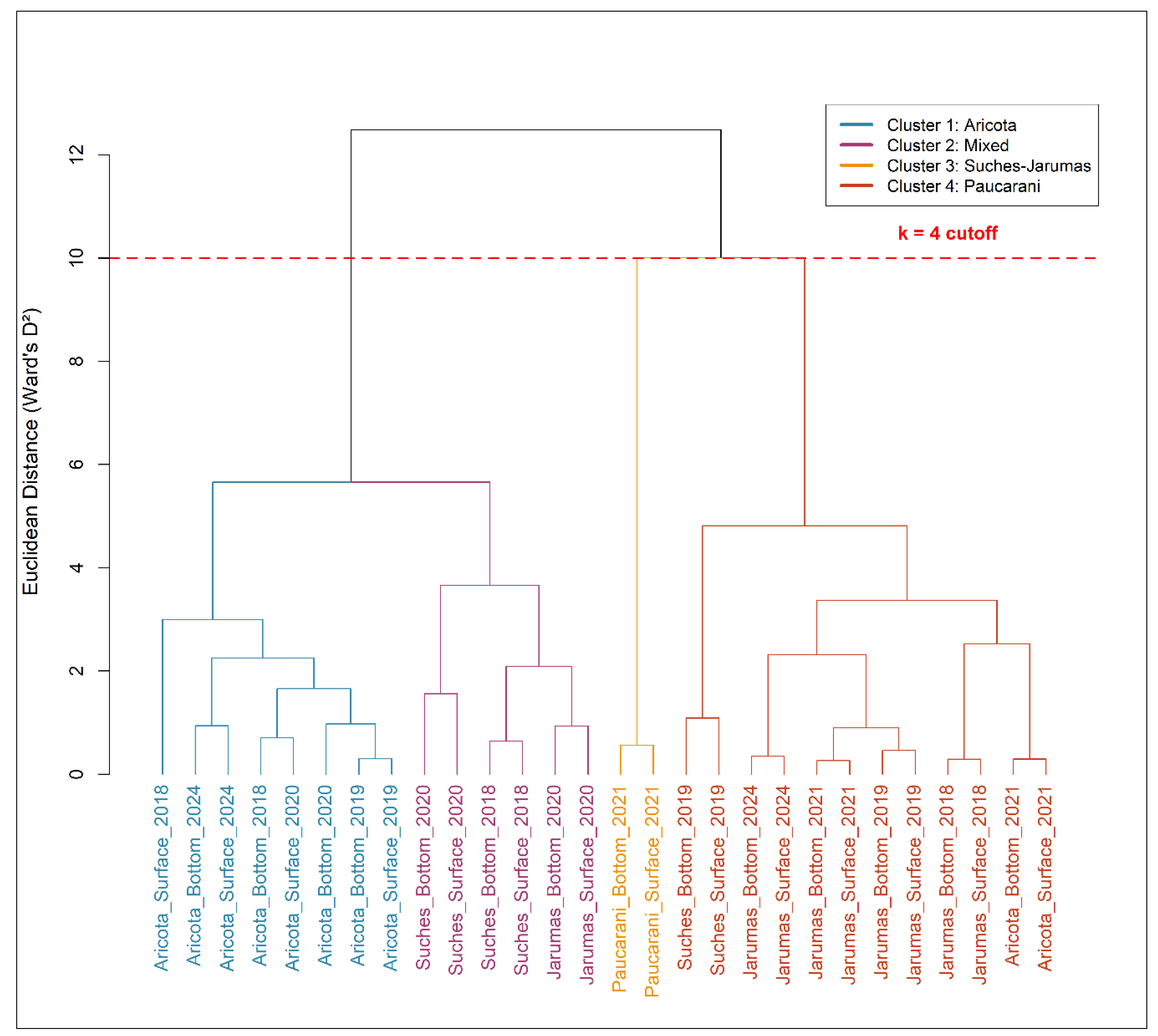
Table S5. Evaluation of optimal cluster solution. Gap statistic based on 100 reference
permutations; silhouette width ranges 0–1 (higher = better-defined clusters); Calinski-Harabasz index
favors between-cluster separation. Bold values indicate k = 4 maximizes clustering quality. Available
at Zenodo (DOI: 10.5281/zenodo.16401603).
3.5.2. Cluster Composition and Characterization
Cluster 1 (n = 8): Aricota 2018–2024 (Persistent Mesotrophy with Moderate Contamination)
Encompasses all Aricota observations across the study period (surface and bottom, 2018–2024). Characterized by elevated TSItsr (56.2 ± 2.0), moderate CD (4.9 ± 0.8 μg L⁻¹), and the lowest CCME-WQI (25.5 ± 3.2), reflecting legacy mining impacts from the Salado River catchment. Despite temporal stability (no significant trends; Section 3.2), Aricota consistently exhibits poorer water quality than other systems, justifying its separation into a distinct functional group.
Cluster 2 (n = 12): Mixed Jarumas–Suches–Aricota 2019–2024 (Improving Moderate Quality)Heterogeneous assemblage spanning Jarumas (n = 6), Suches (n = 4), and recent Aricota observations (n = 2). Shows intermediate TSItsr (50.0 ± 3.2), improved CCME-WQI (43.9 ± 5.1), and low CD (1.7 ± 0.5 μg L⁻¹). This cluster captures systems with moderate anthropogenic pressures (agricultural runoff in Jarumas) or minimal impacts (Suches), representing the "baseline" water quality state for high Andean lakes under contemporary land use.
Cluster 3 (n = 6): Suches–Jarumas 2018–2020 (Optimal Quality)
Groups early-period observations from Suches (2018–2020, n = 4) and Jarumas (2018–2019, n = 2), exhibiting the highest water quality across all metrics: CCME-WQI (52.2 ± 3.0), OWQI (46.2 ± 1.4), lowest CD (0.9 ± 0.2 μg L⁻¹), and moderate TSItsr (55.0 ± 2.8). This cluster represents reference conditions for pristine or minimally impacted high Andean systems, useful for setting restoration targets.
Cluster 4 (n = 2): Paucarani 2021 (Geogenic Metal Contamination)
Exclusive to Paucarani (surface and bottom, 2021), with extreme geogenic metal signatures: HPI (213 ± 15), CD (19.2 ± 2.4 μg L⁻¹), elevated As (mean > 50 μg L⁻¹, data not shown), Pb, and Cd. Paradoxically, TSItsr is low (48.6 ± 0.5, oligotrophic), suggesting that metal toxicity suppresses phytoplankton productivity despite nutrient availability—a pattern documented in other volcanic-hydrothermal systems (e.g., Laguna Verde, Chile; Laguna Colorada, Bolivia). This functional group underscores the need for metal-specific monitoring in geologically active Andean regions.
Table S6. Statistical summary of water quality indices by functional cluster (median ± IQR).
Kruskal–Wallis post-hoc Dunn–Bonferroni letters indicate significantly different medians (α = 0.05).
All seven indices showed significant differences among clusters (p < 0.01), confirming that the k = 4
partition captures ecologically distinct groups. Available at Zenodo (DOI: 10.5281/zenodo.16401603).
3.5.3. Temporal Evolution and Management Implications
Cluster assignments reveal temporal trajectories for individual systems:
- (1)
- Aricota: Persistent Cluster 1 membership throughout 2018–2024 indicates that legacy mining impacts are stable over the decadal timescale, with no evidence of recovery. Management interventions (e.g., sediment remediation, riparian restoration) may be necessary to shift Aricota toward Cluster 2 conditions.
- (2)
- Jarumas: Transitioned from Cluster 3 (2018–2019, optimal quality) to Cluster 2 (2020–2024, moderate quality), suggesting subtle water quality degradation—consistent with the significant CCME-WQI decline detected by Mann-Kendall tests (Section 3.2). This trajectory warrants continued monitoring to prevent further deterioration.
- (3)
- Suches: Maintained Cluster 2–3 membership, reflecting stable, near-pristine conditions befitting its endorheic, remote setting with minimal anthropogenic impacts. Suches serves as a reference ecosystem for assessing change in other systems.
- (4)
- Paucarani: Unique Cluster 4 membership underscores its geogenic outlier status. Management strategies must account for natural metal sources (volcanic-hydrothermal), focusing on minimizing anthropogenic additions (e.g., mining, agriculture) rather than attempting to reduce baseline geogenic loads.
3.5.4. Sensitivity Analysis: Turbidity Approximation
Because turbidity (NTU) was approximated from total suspended solids (TSS) in 34% of samples (n = 10/28), we evaluated sensitivity for indices incorporating turbidity (OWQI, WQIHA). Comparisons between measured and approximated turbidity cases (Supplementary Material S9) revealed mean absolute differences < 5 NTU (< 10% relative error), which propagate to < 2-unit changes in OWQI and WQIHA—well within measurement uncertainty. Cluster assignments remained unchanged when recomputed using measured-turbidity-only cases (n = 18), confirming that conclusions are robust to the approximation within the observed TSS range (5–50 mg L⁻¹).
4. Discussion
High Andean lake systems in southern Peru remain critically undercharacterized despite their hydrological significance for downstream communities reliant on seasonal flows for irrigation, drinking water, and hydropower generation. This study addressed this knowledge gap through a decade-long multimetric synthesis integrating 1,846 field measurements (2015–2024) from four contrasting systems—Aricota, Jarumas, Paucarani, and Suches—spanning 2,800 to 4,600 m elevation on the arid western Andean slope. Seven indices encompassing trophic state (TSItsr, TRIX), comprehensive water quality (OWQI, WQIHA, CCME-WQI), and heavy metal contamination (HPI, CD) were synthesized to test whether multimetric integration reveals spatial divergences and hidden temporal trends undetectable by single-parameter assessments. Our central hypothesis was partially confirmed: spatial heterogeneity indeed dominated the dataset, with lake identity explaining up to 73% of variance (ε² = 0.73 for CCME-WQI, p < 0.001). However, the anticipated "hidden trends" were conspicuously absent, as temporal stability characterized 96.4% of index-stratum combinations (54 out of 56 time series, Mann-Kendall p > 0.05). Most notably, multimetric integration successfully exposed contamination-trophic decoupling—exemplified by Paucarani's paradoxical oligotrophic signature (TSItsr = 48.6) coexisting with extreme metal pollution (HPI = 213 µg L⁻¹) from geogenic sources—that would remain invisible under Peru's current regulatory framework (DS 004-2017-MINAM, ECA-Water).
4.1. Temporal Resilience Versus Spatial Heterogeneity
The pervasive temporal stability observed across 96.4% of index-stratum combinations (54 out of 56 time series showing no significant Mann-Kendall trends, p > 0.05) contrasts sharply with pronounced spatial heterogeneity (ε² = 0.73 for CCME-WQI). This pattern aligns with emerging evidence from tropical high-mountain lakes where interannual consistency, rather than directional change, characterizes decadal-scale dynamics [32]. The apparent resilience likely reflects hydrological and limnophysical stabilization mechanisms specific to these systems, although circulation regimes remain incompletely characterized due to variable depths exceeding 20 m in all four water bodies. Intense ultraviolet radiation at 2,800–4,600 m elevation may suppress phytoplankton biomass even under elevated nutrient concentrations, decoupling trophic response from phosphorus loading—a hypothesis supported by Paucarani's oligotrophic status despite measurable inputs [33]. Moreover, seasonal precipitation regimes in the Central Andes concentrate 60–80% of annual rainfall during austral summer (December–March), yet our analysis—constrained to dry-season sampling—cannot resolve whether wet-season nutrient pulses materially alter water quality trajectories.
In stark contrast, lake identity emerged as the dominant explanatory variable, accounting for 45% of total variance in distance-based redundancy analysis. This spatial divergence is mechanistically traceable to site-specific anthropogenic and geogenic pressure gradients rather than hydrological residence time effects. Aricota exhibited persistent mesotrophy coupled with moderate metal contamination—conditions attributable to geogenic arsenic (0.612 ± 0.06 mg L⁻¹) and phosphorus (1.196 ± 0.134 mg L⁻¹) delivery via the Callazas and Salado rivers draining Cenozoic volcanic headwaters (As = 0.832 ± 0.22 mg L⁻¹, P = 0.404 ± 0.56 mg L⁻¹ in tributary waters), potentially amplified by intensive cage aquaculture operations that have expanded substantially between 2015 and 2024 [34]. Suches Lagoon receives non-natural inflows from groundwater wells operated by Southern Peru Copper Corporation (SPCC), functioning effectively as a water regulation reservoir. Conversely, Jarumas experiences catchment-scale wetland degradation: high-Andean peatlands (bofedales) surrounding the reservoir have contracted visibly in satellite imagery, consistent with climate-driven desiccation and decades of camelid (alpaca, llama) grazing pressure documented across South American altiplano ecosystems [35]. Bofedal deterioration reduces natural water filtration capacity and mobilizes stored nutrients. Paucarani's extreme metal contamination (HPI = 213 µg L⁻¹, CD = 19 µg L⁻¹) originates entirely from hydrothermal spring inflow in the Uchusuma basin, where geogenic arsenic and cadmium leached from silicic volcanic substrates accumulate [36,37]. The absence of anthropogenic mining contamination underscores that naturally occurring geogenic processes and land-use intensification are the proximate drivers.
The two statistically significant temporal trends warrant cautious interpretation. Jarumas exhibited a detectable decline in comprehensive water quality (CCME-WQI: Mann-Kendall τ = −0.235, standardized Z = −2.35, p = 0.019), although the magnitude has not yet triggered reclassification from "good" to "fair" water quality, suggesting gradual deterioration. This subtle degradation trajectory coincides temporally with documented bofedal contraction. Importantly, the absence of corresponding trends in Suches indicates that site-specific stressors can modulate climate-mediated changes. The overwhelming temporal stability contrasts with global narratives of accelerating lake degradation, underscoring that local pressures, rather than regional climate variability, dictate ecological trajectories at decadal scales.
4.2. Multimetric Integration Reveals Contamination-Trophic Decoupling
Paucarani Reservoir epitomizes the diagnostic value of multimetric synthesis. A regulatory assessment relying solely on chlorophyll-a or Secchi depth would classify the system as oligotrophic (TSItsr = 48.6), potentially implying minimal management concern. However, concomitant metal pollution indices expose a contrasting reality: HPI reached 213 µg L⁻¹—exceeding "extreme contamination" thresholds by threefold—driven by arsenic (12.8 ± 4.3 µg L⁻¹) and cadmium (6.2 ± 1.9 µg L⁻¹) concentrations that approach or surpass Peru's Environmental Quality Standards for Category 4 waters (ECA-Water: As = 10 µg L⁻¹, Cd = 4 µg L⁻¹). This contamination-trophic decoupling arises from direct toxic suppression: elevated arsenic and cadmium inhibit photosynthetic enzyme systems in phytoplankton, constraining biomass accumulation despite adequate nutrient availability [38,39]. Geochemical evidence confirms that arsenic partitions into volatile magmatic fluids during Cenozoic arc volcanism, accumulating in shallow geothermal reservoirs that feed Paucarani via fault-controlled discharge [40].
Correlation analysis of the seven indices reveals two statistically and ecologically independent dimensions of water quality deterioration. Metal-based indices (CD and HPI) exhibited very strong positive correlation (r = 0.92, p < 0.001), forming a coherent "contamination axis" driven by geogenic or point-source loading. Conversely, trophic indices (TSItsr and OWQI) showed strong negative correlation (r = −0.91, p < 0.001), reflecting the expected inverse relationship between transparency and productivity. Critically, TSItsr and TRIX correlated only moderately (r = 0.43, p = 0.024), suggesting that chlorophyll-based metrics and nutrient-based metrics capture partially distinct facets of eutrophication—likely because TRIX integrates dissolved oxygen deviations reflecting heterotrophic decomposition as well as autotrophic production [41]. This partial redundancy justifies retaining multiple indices: while some covariation ensures internal consistency, the lack of perfect correlation means each metric contributes unique diagnostic information.
Peru's current regulatory framework (DS 004-2017-MINAM, ECA-Water) relies on single-parameter exceedances to trigger management responses, an approach inadequate for systems experiencing compound stressors. Paucarani technically "complies" with ECA-Water phosphorus standards (< 0.035 mg L⁻¹) yet exhibits ecological impairment via metal toxicity. Conversely, Aricota exceeds phosphorus thresholds due to combined geogenic-volcanic loading and potentially aquaculture-derived inputs. A compliance-only approach would misallocate resources. Multimetric condition assessment enables risk stratification: systems like Paucarani require strategies focused on minimizing additional anthropogenic stressors and protecting human water supply intakes for Tacna's urban population (85% of regional water demand). This shift from "compliance" to "condition" mirrors international best practices under the European Water Framework Directive and Australia's National Water Quality Management Strategy [42,43,44].
4.3. Environmental Drivers and Variance Partitioning
Distance-based redundancy analysis partitioned variance into lake identity (45%), year (8%), and unexplained stochasticity (47%), confirming that site-specific characteristics overwhelm temporal drivers. The primacy of spatial factors aligns with an "environmental envelope" framework wherein each system occupies a relatively stable configuration defined by catchment geology, hydrological connectivity, and land-use pressure. This pattern is consistent with growing evidence that high-mountain tropical lakes can exhibit strong physical buffering that dampens short-term variability in water-column properties [45]. Mechanistically, the prominence of lake identity is most plausibly explained by legacy contamination and internal loading processes. Catchment legacies—whether geogenic metal delivery from volcanic headwaters or chronic diffuse inputs from degraded wetlands—can produce long recovery lags driven by sediment-water feedbacks and internal phosphorus recycling, effectively "locking" systems into persistent states despite partial reductions in external pressure [46,47].
The modest temporal component (8% of explained variance) should not be interpreted as "no change," but as evidence that decadal-scale signals are subtle relative to among-lake contrasts. CAP1 ordination loadings suggest a northwest-to-southeast gradient of gradually improving conditions—consistent with stable land-use patterns. Intriguingly, db-RDA detected no significant stratification effect (surface versus bottom strata), consistent with frequent vertical mixing given depths exceeding 20 m. A critical limitation was the restriction to dry-season sampling for complete-case analysis. Consequently, we cannot assess whether wet-season nutrient pulses from precipitation-driven runoff alter water quality trajectories. Seasonal studies in other Andean systems document 2–3-fold increases in total phosphorus and nitrogen during austral summer, driven by intensified erosion and wetland mobilization [48,49].
4.4. Functional Archetypes as Operational Management Tool
Ward hierarchical clustering on Z-standardized indices identified four functional archetypes with explicit management implications. Risk-typologies are explicitly framed as early-warning devices to target sensitive water bodies before irreversible change occurs [50,51]. Cluster 1 (exclusively Aricota, n = 8 sampling events across 2015–2024) represents persistent mesotrophic-contaminated conditions driven by geogenic volcanic inputs potentially amplified by intensive cage aquaculture expansion. Despite regulatory oversight under Peruvian Aquaculture Law (DL 1195), floating net pen operations expanded without nutrient assimilation infrastructure. This trajectory warrants HIGH management priority: sediment remediation to address legacy phosphorus burial, riparian buffer restoration, and enforceable carrying capacity limits. Critically, Aricota shows no recovery signal across the decade, suggesting potential hysteresis requiring active restoration [52].
Cluster 2 (n = 12 sampling events, mixed systems from 2020–2024) captures systems exhibiting gradual improvement or stability under moderate anthropogenic pressure. This archetype warrants MEDIUM priority through best management practices: enforcing sustainable land-use policies in degraded wetland catchments, revegetating eroded bofedales, and monitoring compliance. Jarumas migrated from Cluster 3 (reference conditions, 2018–2019) to Cluster 2 (2020–2024), signaling subtle degradation consistent with the significant Mann-Kendall decline. This shift occurred before regulatory thresholds were breached, demonstrating early-warning capacity. Intervention at this stage may prevent costlier remediation later [53,54].
Cluster 3 (n = 6 sampling events, early Suches-Jarumas samples from 2018–2019) represents reference conditions: oligotrophic to mesotrophic with low contamination. These conditions serve as restoration targets and warrant LOW management priority (conservation monitoring, biennial sampling frequency). Cluster 4 (n = 2 sampling events, exclusively Paucarani) isolates the geogenic metal anomaly. HPI and CD values exceed all other clusters by an order of magnitude, yet trophic indices remain low—confirming decoupling. Management strategies differ fundamentally: geogenic contamination is irreversible via conventional restoration, necessitating focus on minimizing additional anthropogenic metal inputs and protecting downstream water intakes for Tacna's urban supply (serving 85% of regional population) via pre-treatment (arsenic removal through coagulation-filtration) or alternative sourcing. This archetype warrants MEDIUM-HIGH priority because human exposure pathways remain manageable through infrastructure interventions.
Operationalization for Peru's National Water Authority (ANA) could proceed via quarterly monitoring for high-risk clusters (Clusters 1 and 4), annual monitoring for moderate-risk clusters (Cluster 2), and biennial monitoring for reference clusters (Cluster 3), dynamically adjusting frequency as systems transition.
4.5. Methodological Considerations and Limitations
Several methodological constraints temper the generalizability and precision of our findings. First, turbidity values were approximated from total suspended solids (TSS) concentrations using established regression relationships (r = 0.77–0.96) [55,56], as direct nephelometric turbidity measurements were unavailable for earlier monitoring years. Our TSS range (0.5–37 mg L⁻¹) falls well below thresholds where this approximation degrades (> 800 mg L⁻¹), and sensitivity analysis indicated < 2 WQIHA units uncertainty. Second, chlorophyll-a temporal restriction (2018–2024) constrained trophic index calculation to recent years. This arose because chlorophyll-a measurement requires Secchi depths > 1.5 m and current laboratory detection limits for oligotrophic systems report values as "below detection" rather than quantitative concentrations.
Third, WQIHA parameter coverage reached 85% (17 out of 20 standard parameters), with copper, total dissolved solids, and oils/greases unmeasured. Weight renormalization maintained relative proportions, deemed acceptable by CCME guidelines for > 75% coverage; however, copper's absence may underestimate contamination in Aricota where aquaculture operations contain cupric compounds. Fourth, seasonal bias toward dry-season sampling prevents assessment of wet-season nutrient pulses. Tropical Andean lakes experience pronounced seasonality in precipitation (austral summer receives 60–80% of annual rainfall), driving erosional transport. Fifth, generalizability to other Andean systems warrants cautious extrapolation. Our four lakes span 2,800–4,600 m elevation in southern Peru's arid western slope (300–600 mm annual precipitation). Transferability to wetter regions or different geological substrates remains untested, though mechanistic frameworks apply broadly.
4.6. Management Implications and Early-Warning Thresholds
We propose a joint threshold—CTSI ≥ 60 (transition from mesotrophy to eutrophy) combined with HPI ≥ 100 (significant metal pollution)—as an early-warning criterion for compound stressor risk. This conjunction identifies systems approaching cyanobacterial bloom potential while simultaneously experiencing metal contamination that amplifies ecosystem stress [57,58]. Systems exceeding either threshold individually warrant quarterly monitoring; systems exceeding both thresholds concurrently trigger intensive investigation. This framework acknowledges that single-stressor thresholds are inadequate for predicting ecological outcomes under compound stress [59].
The regulatory gap between Peru's ECA-Water standards (compliance-based, single-parameter) and multimetric condition assessment (integrative, continuous) necessitates policy evolution. We advocate for ANA to adopt a tiered framework: ECA-Water compliance remains the legal floor, but management prioritization is guided by multimetric dashboards. International precedents exist: Europe's Water Framework Directive integrates biological, hydromorphological, and physicochemical indicators [60]. Implementing a similar approach in Peru would require: (i) establishing Andean-specific reference conditions via paleolimnological reconstruction or pristine-lake surveys, (ii) deriving pressure-state relationships through gradient studies, and (iii) validating thresholds via whole-lake experiments.
Resource allocation should follow archetype-specific strategies. HIGH priority (Cluster 1, Aricota): allocate ~40% of regional restoration budget to sediment phosphorus inactivation, aquaculture carrying capacity enforcement, and riparian buffer installation—estimated cost ~USD 2–3 million over 5 years. MEDIUM-HIGH priority (Cluster 4, Paucarani): invest ~30% in water supply infrastructure bypassing geogenic contamination—pre-treatment via arsenic removal serving Tacna's 85% regional water demand—estimated cost ~USD 1.5 million. MEDIUM priority (Cluster 2): maintain current trajectories via best management practices enforcement (cost-neutral). LOW priority (Cluster 3): conservation monitoring (~10% of budget, USD 100,000 annually).
Specific recommendations for ANA include: (1) expand chlorophyll-a monitoring to wet seasons via fluorometric probes with enhanced detection limits or satellite remote sensing (Sentinel-2 algorithms calibrated with n ≥ 30 samples); (2) implement archetype-specific monitoring frequencies; (3) adopt a minimum three-index dashboard (TRIX, CCME-WQI, HPI) for routine assessments; (4) establish early-warning protocols triggering rapid-response investigations when systems transition cluster boundaries; (5) pilot restoration at Aricota to test intervention effectiveness; (6) capacity building via training workshops for regional ANA offices. Cost-benefit analysis supports multimetric monitoring despite marginal expense increases (~15% more laboratory analyses). Early intervention is consistently more cost-effective than crisis response: preventing a cyanobacterial bloom via nutrient management costs USD 50,000–100,000 per lake annually, whereas treating contaminated drinking water costs USD 500,000–1,000,000.
5. Conclusions
This decade-long multimetric assessment of four high Andean lakes (Aricota, Jarumas, Paucarani, Suches) spanning 2,800–4,600 m elevation demonstrates that spatial heterogeneity overwhelmingly dominates temporal variability at decadal scales. Across 1,846 monitoring records (2015–2024), lake identity consistently emerged as the primary determinant of condition (ε² = 0.73 for CCME-WQI), while 96.4% of index-stratum combinations exhibited no significant temporal trends. These results partially validate the central hypothesis: the multimetric approach revealed contamination-trophic decoupling that would be overlooked by single-parameter assessments; however, the expected "hidden trends" were largely absent, indicating substantial temporal resilience.
Only Jarumas showed significant degradation (CCME-WQI: Mann-Kendall τ = −0.235, Z = −2.35, p = 0.019), consistent with documented bofedal degradation. Spatial divergence was unequivocal (p < 0.001 all indices, ε² = 0.42–0.73). Distance-based redundancy analysis partitioned substantially more variance to lake identity (45%) than to year (8%), indicating that persistent site-specific drivers—catchment geology, anthropogenic legacies, hydrological setting—structure condition more strongly than interannual climate variability. Metal stress suppresses phytoplankton productivity, weakening nutrient-chlorophyll linkages.
Ward clustering integrated the seven indices into four functional archetypes with direct operational value. Cluster 1 (Aricota, no recovery 2015–2024) warrants HIGH priority (sediment remediation, aquaculture limits, USD 2–3M/5 years, 40% budget). Cluster 2 (mixed systems) warrants MEDIUM priority (best practices, cost-neutral), with Jarumas transition Cluster 3→2 demonstrating early-warning capacity. Cluster 3 (reference conditions) warrants LOW priority (biennial monitoring, USD 100K annually, 10% budget). Cluster 4 (Paucarani geogenic anomaly) warrants MEDIUM-HIGH priority protecting 85% Tacna supply (pre-treatment, USD 1.5M, 30% budget).
Proposed compound threshold (CTSI ≥ 60 + HPI ≥ 100) addresses ECA-Water inadequacy for distributed stressors. Archetype-based monitoring (quarterly Clusters 1,4; annual Cluster 2; biennial Cluster 3) optimizes resources. Despite limitations—dry-season bias, chlorophyll-a detection challenges, depths > 20 m precluding definitive polymictic classification—multimetric framework demonstrates diagnostic superiority. Integration with Sentinel-2 remote sensing (requiring n ≥ 30 calibration samples) positions this as scalable template for ~200 Peru lakes and ~15,000 tropical Andean systems requiring proactive stewardship under intensifying pressures.
Author Contributions
Conceptualization, methodology, writing, investigation, project administration, JACA; methodology, EMLS; software, DGRO; validation, YMCD, DGRO, EMLS and KADL; formal analysis, EMLS; investigation, YMCD, DGRO and KADL; resources, EMLS; data curation, EMLS, KADL; writing—original draft, YMCD and DGRO; writing—review and editing, DGRO, YMCD; visualization and supervision, EMLS. All authors have read and approved the published version of the manuscript.
Data Availability Statement
The datasets and R scripts supporting the results of this study are available on Zenodo, under the Creative Commons Attribution 4.0 license, with the DOI identifier: 10.5281/zenodo.16401603.
Acknowledgments
In this section, you can acknowledge any support given which is not covered by the author contribution or funding sections. This may include administrative and technical support, or donations in kind (eg, materials used for experiments). Where GenAI has been used for purposes such as generating text, data, or graphics, or for study design, data collection, analysis, or interpretation of data, please add “During the preparation of this manuscript/study, the author(s) used [tool name, version information] for the purposes of [description of use]. The authors have reviewed and edited the output and take full responsibility for the content of this publication.”.
References
- Yao, F; Livneh, B; Rajagopalan, B; Wang, J; Crétaux, JF; Wada, Y; et al. Satellites reveal widespread decline in global lake water storage. Science (1979) [Internet] Available from. 2023, 380(6646), 743–9. [Google Scholar] [CrossRef] [PubMed]
- Meyer, MF; Topp, SN; King, T V; Ladwig, R; Pilla, RM; Dugan, HA; et al. National-scale remotely sensed lake trophic state from 1984 through 2020. Sci Data [Internet]. Jan 2024, 11. Available online: https://www.nature.com/articles/s41597-024-02921-0.
- Yin, Y; Yang, K; Gao, M; Wei, J; Zhong, X; Jiang, K; et al. Declined nutrients stability shaped by water residence times in lakes and reservoirs under climate change. Science of The Total Environment [Internet] 2024, 953, 176098. Available online: https://linkinghub.elsevier.com/retrieve/pii/S0048969724062545. [CrossRef]
- Dodds, WK. Trophic state, eutrophication and nutrient criteria in streams. Trends Ecol Evol. 2007, 22(12), 669–76. [Google Scholar] [CrossRef]
- Klippel, G; Macêdo, RL; Branco, CWC. Comparison of different trophic state indices applied to tropical reservoirs. Lakes & Reservoirs: Science, Policy and Management for Sustainable Use 2020, 25(2), 214–29. [Google Scholar] [CrossRef]
- Cunha, DGF; Finkler, NR; Lamparelli, MC; Calijuri M do, C; Dodds, WK; Carlson, RE. Characterizing Trophic State in Tropical/Subtropical Reservoirs: Deviations among Indexes in the Lower Latitudes. Environ Manage 2021, 68(4), 491–504. [Google Scholar] [CrossRef]
- Uddin, MdG; Nash, S; Olbert, AI. A review of water quality index models and their use for assessing surface water quality. Ecol Indic [Internet] 2021, 122, 107218. Available online: https://linkinghub.elsevier.com/retrieve/pii/S1470160X20311572. [CrossRef]
- Biedunkova, O; Kuznietsov, P. Dataset on heavy metal pollution assessment in freshwater ecosystems. Sci Data [Internet]. Nov 2024, 11. Available online: https://www.nature.com/articles/s41597-024-04116-z.
- Murray, J; Guzmán, S; Tapia, J; Nordstrom, DK. Silicic volcanic rocks, a main regional source of geogenic arsenic in waters: Insights from the Altiplano-Puna plateau, Central Andes. Chem Geol. 2023, 629, 121473. [Google Scholar] [CrossRef]
- Simon, IJP; Pfaff, K; Navarre-Sitchler, A; Crespo, J; Holley, E; Vanzin, G; et al. Geological and anthropogenic contributions of metal(loid)s in the artisanal and small-scale mining-impacted Ocoña watershed of Arequipa, Peru. Applied Geochemistry 2024, 168, 106028. [Google Scholar] [CrossRef]
- Ayala Izurieta, JE; Beltrán Dávalos, AA; Jara Santillán, CA; Godoy Ponce, SC; Van Wittenberghe, S; Verrelst, J; et al. Spatial and Temporal Analysis of Water Quality in High Andean Lakes with Sentinel-2 Satellite Automatic Water Products. Sensors [Internet] 2023, 23(21), 8774. Available online: https://www.mdpi.com/1424-8220/23/21/8774. [CrossRef]
- Campero, M; Balseiro, E; Fernández, CE; Modenutti, B; Prado, PE; Rivera-Rondon, CA; et al. Andean lakes: endangered by natural and anthropogenic threats. Inland Waters 2024, 14(4), 352–68. [Google Scholar] [CrossRef]
- Bello, C; Suarez, W; Drenkhan, F; Vega-Jácome, F. Hydrological impacts of dam regulation for hydropower production: The case of Lake Sibinacocha, Southern Peru. J Hydrol Reg Stud. 2023, 46, 101319. [Google Scholar] [CrossRef]
- García-Avila, F; Loja-Suco, P; Siguenza-Jeton, C; Jiménez-Ordoñez, M; Valdiviezo-Gonzales, L; Cabello-Torres, R; et al. Evaluation of the water quality of a high Andean lake using different quantitative approaches. Ecol Indic. 2023, 154, 110924. [Google Scholar] [CrossRef]
- R Core Team. R: A Language and Environment for Statistical Computing; The R Foundation.: Viena (Austria), 2024; Available online: https://www.R-project.org/.
- Choque-Quispe, D; Froehner, S; Palomino-Rincón, H; Peralta-Guevara, DE; Barboza-Palomino, GI; Kari-Ferro, A; et al. Proposal of a Water-Quality Index for High Andean Basins: Application to the Chumbao River, Andahuaylas, Peru. Water (Basel) 2022, 14(4), 654. [Google Scholar] [CrossRef]
- Cunha, DGF; Calijuri, MDC; Lamparelli, MC. A trophic state index for tropical/subtropical reservoirs (TSItsr). Ecol Eng [Internet] 2013, 60, 126–34. Available online: https://linkinghub.elsevier.com/retrieve/pii/S0925857413003091. [CrossRef]
- OCDE. Eutrophisation des eaux. Métodes de surveillance, d’evaluation et de lutte; Paris, 1982. [Google Scholar]
- Vollenweider, RA; Giovanardi, F; Montanari, G; Rinaldi, A. Characterization of the trophic conditions of marine coastal waters with special reference to the NW Adriatic Sea: proposal for a trophic scale, turbidity and generalized water quality index. Environmetrics 1998, 9(3), 329–57. [Google Scholar] [CrossRef]
- Winslow, LA; Zwart, JA; Batt, RD; Dugan, HA; Woolway, RI; Corman, JR; et al. LakeMetabolizer: an R package for estimating lake metabolism from free-water oxygen using diverse statistical models. Inland Waters 2016, 6(4), 622–36. [Google Scholar] [CrossRef]
- Packman, JJ; Coming, KJ; Booth, DB. Using turbidity to determine total suspended solids in urbanizing streams in the Puget lowlands. Managing Change in Water Resources and the Environment, Canadian Water Resources Association annual meeting, Vancouver, 1999; pp. 158–65. [Google Scholar]
- Delegido, J; Urrego, P; Vicente, E; Sòria-Perpinyà, X; Soria, JM; Pereira-Sandoval, M; et al. Turbidez y profundidad de disco de Secchi con Sentinel-2 en embalses con diferente estado trófico en la Comunidad Valenciana. Revista de Teledetección 2019, (54), 15. [Google Scholar] [CrossRef]
- Wu, JL; Ho, CR; Huang, CC; Srivastav, A; Tzeng, JH; Lin, YT. Hyperspectral Sensing for Turbid Water Quality Monitoring in Freshwater Rivers: Empirical Relationship between Reflectance and Turbidity and Total Solids. Sensors 2014, 14(12), 22670–88. [Google Scholar] [CrossRef]
- de Oliveira, ARM; Borges, AC; Matos, AT; Nascimento, M. ESTIMATION ON THE CONCENTRATION OF SUSPENDED SOLIDS FROM TURBIDITY IN THE WATER OF TWO SUB-BASINS IN THE DOCE RIVER BASIN. Engenharia Agrícola 2018, 38(5), 751–9. [Google Scholar] [CrossRef]
- CCME. Canadian Water Quality Guidelines for the Protection of Aquatic life: Canadian Water Quality Index 1.0 Technical Report [Internet]. 2001. Available from: chromeextension:// oemmndcbldboiebfnladdacbdfmadadm/https://ccme.ca/en/res/wqimanualen.pdf.
- Cude, CG. OREGON WATER QUALITY INDEX A TOOL FOR EVALUATING WATER QUALITY MANAGEMENT EFFECTIVENESS^1. JAWRA Journal of the American Water Resources Association [Internet] 2001, 37(1), 125–37. Available online: https://onlinelibrary.wiley.com/doi/10.1111/j.1752-1688.2001.tb05480.x. [CrossRef]
- Prasad, B; Bose, J. Evaluation of the heavy metal pollution index for surface and spring water near a limestone mining area of the lower Himalayas. Environmental Geology 2001, 41(1–2), 183–8. [Google Scholar] [CrossRef]
- Hakanson, L. An ecological risk index for aquatic pollution control.a sedimentological approach. Water Res. 1980, 14(8), 975–1001. [Google Scholar] [CrossRef]
- Helsel, DR; Hirsch, RM; Ryberg, KR; Archfield, SA; Gilroy, EJ. Statistical methods in water resources [Internet]. 2020. Available online: https://pubs.usgs.gov/publication/tm4A3.
- R Core Team. R: A language and environment for statistical computing. 2023. Available online: https://www.R-project.org.
- Flanagin, A; Bibbins-Domingo, K; Berkwits, M; Christiansen, SL. Nonhuman “Authors” and Implications for the Integrity of Scientific Publication and Medical Knowledge. JAMA 2023, 329(8), 637. [Google Scholar] [CrossRef] [PubMed]
- Meyer, MF; Topp, SN; King, T V.; Ladwig, R; Pilla, RM; Dugan, HA; et al. National-scale remotely sensed lake trophic state from 1984 through 2020. Sci Data 2024, 11(1), 77. [Google Scholar] [CrossRef] [PubMed]
- Aguilera, X; Lazzaro, X; Coronel, JS. Tropical high-altitude Andean lakes located above the tree line attenuate UV-A radiation more strongly than typical temperate alpine lakes. Photochemical & Photobiological Sciences 2013, 12(9), 1649–57. [Google Scholar]
- Bundschuh, J; Armienta, MA; Birkle, P; Bhattacharya, P; Matschullat, J; Mukherjee, AB. Natural Arsenic in Groundwaters of Latin America; Bundschuh, J, Armienta, MA, Birkle, P, Bhattacharya, P, Matschullat, J, Mukherjee, AB, Eds.; CRC Press, 1997. [Google Scholar]
- Yager, K; Prieto, M; Meneses, RI. Reframing Pastoral Practices of Bofedal Management to Increase the Resilience of Andean Water Towers. Mt Res Dev 2021, 41(4). [Google Scholar] [CrossRef]
- Pavez, M; Brasse, H; Kapinos, G; Díaz, D; Lara, LE; Schill, E. Magma storage and transfer in the Villarrica volcanic chain, South Chile: MT insights into volcano-tectonic interactions. Journal of Volcanology and Geothermal Research 2023, 439, 107832. [Google Scholar] [CrossRef]
- Bia, G; García, MG; Cosentino, NJ; Borgnino, L. Dispersion of arsenic species from highly explosive historical volcanic eruptions in Patagonia. Science of The Total Environment 2022, 853, 158389. [Google Scholar] [CrossRef] [PubMed]
- Nawaz, A; Šotek, PE; Molnárová, M. Reciprocal Effects of Metal Mixtures on Phytoplankton. Phycology 2024, 4(1), 117–38. [Google Scholar] [CrossRef]
- Biamont-Rojas, IE; Cardoso-Silva, S; Figueira, RCL; Kim, BSM; Alfaro-Tapia, R; Pompêo, M. Spatial distribution of arsenic and metals suggest a high ecotoxicological potential in Puno Bay, Lake Titicaca, Peru. Science of The Total Environment 2023, 871, 162051. [Google Scholar] [CrossRef]
- Murray, J; Guzmán, S; Tapia, J; Nordstrom, DK. Silicic volcanic rocks, a main regional source of geogenic arsenic in waters: Insights from the Altiplano-Puna plateau, Central Andes. Chem Geol. 2023, 629, 121473. [Google Scholar] [CrossRef]
- García-Avila, F; Loja-Suco, P; Siguenza-Jeton, C; Jiménez-Ordoñez, M; Valdiviezo-Gonzales, L; Cabello-Torres, R; et al. Evaluation of the water quality of a high Andean lake using different quantitative approaches. Ecol Indic. 2023, 154, 110924. [Google Scholar] [CrossRef]
- Vitecek, S; Johnson, R; Poikane, S. Assessing the Ecological Status of European Rivers and Lakes Using Benthic Invertebrate Communities: A Practical Catalogue of Metrics and Methods. Water (Basel) 2021, 13(3), 346. [Google Scholar] [CrossRef]
- Chidiac, S; El Najjar, P; Ouaini, N; El Rayess, Y; El Azzi, D. A comprehensive review of water quality indices (WQIs): history, models, attempts and perspectives. Rev Environ Sci Biotechnol. 2023, 22(2), 349–95. [Google Scholar] [CrossRef]
- Lukhabi, DK; Mensah, PK; Asare, NK; Pulumuka-Kamanga, T; Ouma, KO. Adapted Water Quality Indices: Limitations and Potential for Water Quality Monitoring in Africa. Water (Basel) 2023, 15(9), 1736. [Google Scholar] [CrossRef]
- Mosquera, P V.; Batalla, M; Hampel, H; Vázquez, RF; Catalan, J. Mixing regimes in tropical high-mountain Andean lakes. Limnol Oceanogr. 2025, 70(10), 2872–92. [Google Scholar] [CrossRef]
- Carleton, JN; Lee, SS. Modeling lake recovery lag times following influent phosphorus loading reduction. Environmental Modelling & Software 2023, 162, 105642. [Google Scholar] [CrossRef]
- Chen, M; Li, X; de Klein, J; Janssen, ABG; Du, X; Lei, Q; et al. Long-term responses of internal environment dynamics in a freshwater lake to variations in external nutrient inputs: A model simulation approach. Science of The Total Environment 2024, 951, 175514. [Google Scholar] [CrossRef] [PubMed]
- Fernández, R; Alcocer, J; Oseguera, LA; Zuñiga-Ramos, CA; Vilaclara, G. Phytoplankton Communities’ Seasonal Fluctuation in Two Neighboring Tropical High-Mountain Lakes. Plants 2024, 13(21), 3021. [Google Scholar] [CrossRef]
- Pak, HY; Chuah, CJ; Tan, ML; Yong, EL; Snyder, SA. A framework for assessing the adequacy of Water Quality Index – Quantifying parameter sensitivity and uncertainties in missing values distribution. Science of The Total Environment 2021, 751, 141982. [Google Scholar] [CrossRef] [PubMed]
- Keith, DA; Ferrer-Paris, JR; Nicholson, E; Bishop, MJ; Polidoro, BA; Ramirez-Llodra, E; et al. A function-based typology for Earth’s ecosystems. Nature 2022, 610(7932), 513–8. [Google Scholar] [CrossRef] [PubMed]
- Politi, E; Cutler, MEJ; Carvalho, L; Rowan, JS. A global typological approach to classify lakes based on their eutrophication risk. Aquat Sci. 2024, 86(2), 52. [Google Scholar] [CrossRef]
- Perrotta, BG; Kidd, KA; Campbell, KM; Croteau, MN; Kane, TJ; Marcarelli, AM; et al. Metal-rich lacustrine sediments from legacy mining perpetuate copper exposure to aquatic-riparian food webs. Integr Environ Assess Manag 2025, 21(2), 414–24. [Google Scholar] [CrossRef]
- Okechi, JK; Peoples, N; Nyamweya, CS; Orina, PS; Cooperman, MS; Kaufman, L. Effects of Nile tilapia (Oreochromis niloticus) cage aquaculture on water quality in the world’s largest tropical lake. J Great Lakes Res. 2025, 51(3), 102576. [Google Scholar] [CrossRef]
- Campero, M; Balseiro, E; Fernández, CE; Modenutti, B; Prado, PE; Rivera-Rondon, CA; et al. Andean lakes: endangered by natural and anthropogenic threats. Inland Waters 2024, 14(4), 352–68. [Google Scholar] [CrossRef]
- Skarbøvik, E; Gyritia Madsen van’t Veen, S; Lannergård, EE; Wenng, H; Stutter, M; Bieroza, M; et al. Comparing in situ turbidity sensor measurements as a proxy for suspended sediments in North-Western European streams. Catena (Amst) 2023, 225, 107006. [Google Scholar] [CrossRef]
- Kim, J; Kwon, S; Chung, S; Kim, Y; Do. Turbidity and suspended sediment relationship based on sediment composition and particle size distribution. Sci Rep. 2025, 15(1), 16286. [Google Scholar] [CrossRef]
- Hu, M; Ma, R; Xue, K; Cao, Z; Chen, X; Xiong, J; et al. A dataset of trophic state index for nation-scale lakes in China from 40-year Landsat observations. Sci Data 2024, 11(1), 659. [Google Scholar] [CrossRef]
- Badeenezhad, A; Soleimani, H; Shahsavani, S; Parseh, I; Mohammadpour, A; Azadbakht, O; et al. Comprehensive health risk analysis of heavy metal pollution using water quality indices and Monte Carlo simulation in R software. Sci Rep. 2023, 13(1), 15817. [Google Scholar] [CrossRef]
- Kong, X; Determann, M; Andersen, TK; Barbosa, CC; Dadi, T; Janssen, ABG; et al. Synergistic Effects of Warming and Internal Nutrient Loading Interfere with the Long-Term Stability of Lake Restoration and Induce Sudden Re-eutrophication. Environ Sci Technol. 2023, 57(9), 4003–13. [Google Scholar] [CrossRef]
- Vitecek, S; Johnson, R; Poikane, S. Assessing the Ecological Status of European Rivers and Lakes Using Benthic Invertebrate Communities: A Practical Catalogue of Metrics and Methods. Water (Basel) 2021, 13(3), 346. [Google Scholar] [CrossRef]
Table 1.
Sampling station metadata for the southern Peru high-altitude monitoring network.
| Water Body | Station | Stratum | Coordinates (UTM 19S, WGS84) | Elev. (m) | Watershed | Period |
| Suches | LSuch1 | S / B | 350673E, 8127271N | 4,570 | Locumba | 2015–2024 |
| LSuch2 | S / B | 352715E, 8128900N | 4,570 | Locumba | 2015–2024 | |
| Aricota | LAric1 | S / B | 360597E, 8079983N | 2,800 | Locumba | 2015–2024 |
| LAric2 | S / B | 363130E, 8080455N | 2,800 | Locumba | 2015–2024 | |
| LAric3 | S / B | 364768E, 8081585N | 2,800 | Locumba | 2015–2024 | |
| Jarumas | EJaru1 | S / B | 399237E, 8079387N | 4,500 | Sama | 2015–2021, 2024 |
| EJaru2 | S / B | 398433E, 8080137N | 4,500 | Sama | 2015–2021, 2024 | |
| Paucarani | EPauc1 | S / B | 418026E, 8061405N | 4,500 | Uchusuma | 2015–2017, 2021, 2024 |
| EPauc2 | S / B | 418817E, 8061230N | 4,500 | Uchusuma | 2015–2017, 2021, 2024 |
Notes: All coordinates are reported in WGS84 datum, UTM Zone 19S projection. S = Surface stratum (≈0.3 m depth); B = Bottom stratum (optical depth = Secchi disk depth). Suches, Aricota, and Jarumas are classified under Peruvian Environmental Quality Standards for Water Category 4-E1 (Conservation of Aquatic Ecosystems in Lakes and Lagoons; DS 004-2017-MINAM). Paucarani Reservoir is classified under Category 1A2 (Waters Intended for Human Consumption with Conventional Treatment), reflecting its strategic role in potable water supply for Tacna city. Monitoring periods reflect years with at least one complete sampling campaign; temporal gaps in Jarumas (2022–2023) and Paucarani (2018–2020, 2022–2023) are documented in the main text. Elevation data were derived from SRTM 30m digital elevation model.
Disclaimer/Publisher’s Note: The statements, opinions and data contained in all publications are solely those of the individual author(s) and contributor(s) and not of MDPI and/or the editor(s). MDPI and/or the editor(s) disclaim responsibility for any injury to people or property resulting from any ideas, methods, instructions or products referred to in the content. |
© 2026 by the authors. Licensee MDPI, Basel, Switzerland. This article is an open access article distributed under the terms and conditions of the Creative Commons Attribution (CC BY) license (http://creativecommons.org/licenses/by/4.0/).
Copyright: This open access article is published under a Creative Commons CC BY 4.0 license, which permit the free download, distribution, and reuse, provided that the author and preprint are cited in any reuse.


