Submitted:
01 February 2026
Posted:
03 February 2026
You are already at the latest version
Abstract
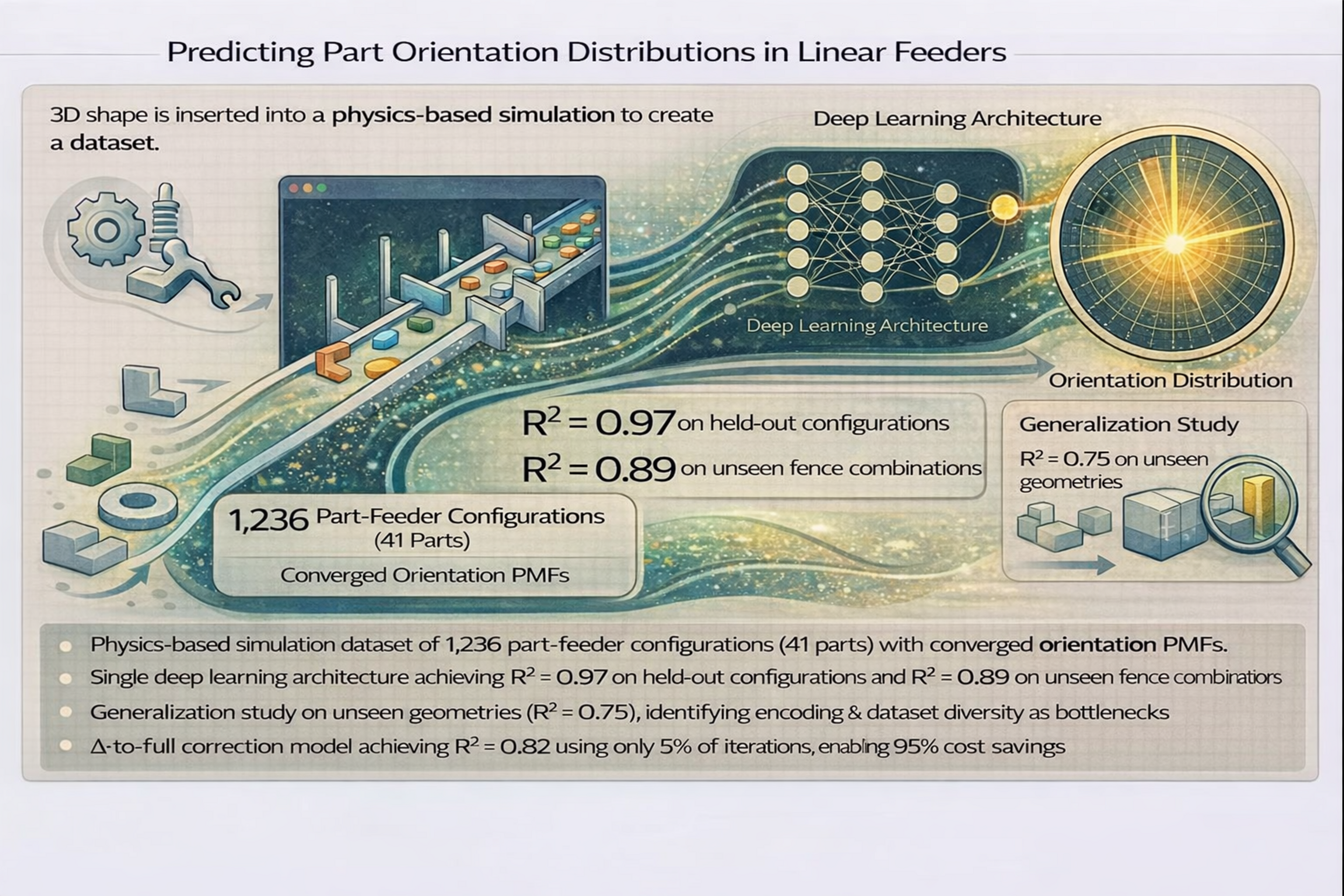
Designing linear conveyor feeders with passive fences for automated part orientation remains largely trial-and-error because the final orientation distribution is difficult to predict reliably before physical testing. We present a simulation-driven deep learning pipeline that predicts the full distribution of final in-plane orientations for extruded, z-axis-symmetric parts interacting with linear feeders containing up to two straight or curved fences. Using Bullet physics-based simulation in CoppeliaSim, we generate 1,048 main part--feeder samples across 38 part geometries, plus 78 fence-generalization and 110 unseen-part samples for a total of 1,236 (41 unique parts), and train regression networks and a Variational Autoencoder, or VAE, to predict 360-bin orientation probability distributions. On known parts, the regression model achieves high accuracy on held-out test configurations, R² on circular CDFs = 0.97 ± 0.05, and on unseen fence combinations, R² on circular CDFs = 0.89 ± 0.11. Generalization to previously unseen part geometries is more challenging, with R² on circular CDFs = 0.75 ± 0.18, indicating that geometric representation and dataset diversity are primary limitations. We also evaluate VAE reconstruction on datasets generated from simulations at different iteration counts, 5--100% of 1000 iterations in 5% increments. While within-level reconstruction remains high, cross-convergence evaluation shows partial-iteration PMFs are far from fully converged labels in this dataset (overall CDF R² = 0.01 at 5%, 0.32 at 50%, and 0.87 at 75%), so reduced-iteration simulations do not substitute for full convergence here. Overall, the proposed approach provides a data-driven foundation for feeder analysis and design, with future work focusing on improved geometric generalization and physical validation for industrial deployment.
Keywords:
linear feeders
; part orientation distribution
; physics-based simulation
; deep learning
; Variational Autoencoder
; manufacturing automation
1. Introduction
Automated part feeding and orientation are essential in modern high-volume manufacturing and assembly lines. These processes directly affect throughput, cost, and product quality. Conveyor systems with passive geometric features, such as fences that act as geometric barriers along the conveyor, are a robust and cost-effective way to orient parts. They do not need complex robotics or sensors. However, designing these linear feeders is difficult. Engineers must choose the right type, number, and configuration of fences for each part shape to get the desired orientation. This is a major engineering challenge, particularly for complex 3D parts and intricate feeder designs. Traditional design relies on expert intuition and trial-and-error [1], often leading to suboptimal designs and long development times. While physical simulations and algorithmic methods have been explored [2,3,4], they often struggle with complex part–fence interactions, require significant computation for each new design, and may not predict feeder performance reliably before testing. This study focuses specifically on predicting orientation distributions for z-axis-symmetric 3D parts, extruded 2D shapes, interacting with linear feeders containing up to two straight or curved fences, laying the groundwork for more complex scenarios. Representative part–fence configurations are shown in Figure 1.
Current solutions, such as dynamic simulations, geometric algorithms, and early machine learning methods, have improved the field. However, there is still a major gap. To the authors’ knowledge, there are no widely adopted automated tools that accurately predict the full probability distribution of final part orientations, that is, the likelihood of a part ending in any possible orientation after passing through the feeder, for a given part and feeder design across diverse geometries and fence configurations. Predicting this full orientation distribution, rather than just a single likely outcome, is crucial for robust design and performance assessment. Furthermore, the high computational cost of simulation hinders exploration, and there are few methods to optimize this data-generation process. Researchers also need methods that use these predictions to help automate the feeder design process, not just analyze it. Most simulation tools require many runs for each design, and current machine learning approaches do not generalize well to new part shapes or give a strong measure of part–feeder compatibility.
This research proposes a new approach to fill this gap. We combine physics-based simulation with deep learning, using Variational Autoencoders, or VAEs, and regression models. These models learn the mapping between part geometry, fence configuration, and the resulting orientation distribution, represented as a discrete 360-bin Probability Mass Function, PMF, and its circular CDF. A key aspect is exploring the VAE not only for learning joint representations of parts, feeders, and orientation PMFs and CDFs, but also as a first step toward more efficient simulation pipelines. Specifically, we investigate training on less converged simulation data, 5–100% of 1000 iterations in 5% increments, and report reconstruction performance as a function of convergence level, alongside a cross-convergence evaluation on the 100% holdout. This test remains limited to reconstruction on the same configuration set. The PMF assigns probability to each orientation bin, while the CDF summarizes cumulative probability around the circle. This learned representation, together with direct regression models, is used to predict feeder performance and support a more informed design process, serving as a step toward automation.
The research objectives are:
- 1.
- Generate a comprehensive dataset of part-orientation distributions using physics-based simulation in CoppeliaSim for z-axis-symmetric 3D parts interacting with linear feeders.
- 2.
- Develop and evaluate deep learning models, regression networks, and VAE, to predict orientation distributions with target accuracy on unseen configurations.
- 3.
- Investigate the VAE’s ability to learn latent representations from simulations at different iteration counts, 5–100%, quantifying within-level and cross-convergence reconstruction performance to assess whether partial simulations can support cost reduction.
- 4.
- Evaluate a delta-to-full correction model that predicts the update from partial to fully converged PMFs using multiple checkpoints, under part-level and configuration-level splits.
- 5.
- Assess model generalization to unseen feeder configurations and new part geometries, quantifying performance degradation and identifying limiting factors.
This research uses a new simulation-driven deep learning approach to solve these challenges. The following sections explain the methods used, including the simulation setup; data representation with Discrete Fourier Transform (DFT) for parts, one-hot encoding for feeders, and PMF/CDF for distributions; model architectures with fully connected networks and VAE; and evaluation strategies. We compare different modeling approaches and test their performance on various datasets, including new parts and robustness to changes. The discussion explains the results, points out limitations, and suggests future research for real-world use. The paper is organized as follows: Section 2 reviews related work. Section 3 explains data generation, representation, and model development. Section 4 presents model results. Section 5 discusses the results, limitations, and future work. Section 6 summarizes the main contributions and findings.
Key contributions.
- Dataset: A simulation-driven dataset of 1,236 part–feeder configurations, split into Main, Test, Fences, and Parts datasets, with 360-bin orientation PMFs and CDFs for extruded 2D parts and up to two fences.
- Regression models: Models that predict full orientation distributions, achieving on circular CDFs of 0.97 on held-out test configurations and 0.89 on unseen fence combinations for known parts, with a marked drop on unseen parts to 0.75.
- VAE convergence study: A VAE reconstruction study across partial-iteration datasets (5–100% in 5% increments) showing high within-level reconstruction () but weak cross-convergence to 100% labels (overall CDF = 0.01 at 5%, 0.32 at 50%, and 0.87 at 75%), consistent with partial-iteration PMFs remaining far from fully converged distributions.
- Delta-to-full correction: A correction model that predicts the update from partial PMFs to the 100% PMF, improving low-iteration performance (e.g., at 5% for unseen parts vs. a negative baseline), with a full 5% sweep reported in Supplementary Section S11.
Scope: We consider extruded 2D, z-axis-symmetric parts and up to two straight/curved fences; broader 3D parts and more complex feeders are discussed in Section 5.
1.1. Problem Formulation
We consider a supervised prediction task from part and feeder descriptors to an orientation distribution. For each configuration, the input vector is
where encodes the part geometry using DFT coefficients and encodes the fence types and angles. The target output is the discrete orientation distribution obtained from simulation:
where the PMF assigns probability to each bin and the CDF is its circular cumulative version. Regression models learn a mapping , while the VAE learns a joint latent representation to reconstruct and evaluate reconstruction fidelity.
2. Related Work
Researchers have long studied how to feed and orient parts in automated assembly efficiently. This challenge, called the part feeding problem, has existed since the start of automation [1]. As mass production has grown and manual labor has become more costly and limited, the need for strong automated solutions has increased [1]. Over the years, many strategies have been developed. These range from simple mechanical devices to advanced simulation-based and machine learning approaches. This review groups these developments by theme. It highlights key advances, ongoing limitations, and the specific research gap this work addresses.
2.1. Early Mechanical and Robotic Solutions
Early solutions focused on mechanical design and robotics. Vibratory Bowl Feeders, VBFs, became common. They use vibrations and geometric traps like gates, fences, and grooves along a helical track to passively orient parts [1,5]. VBFs work well for specific parts, but their design is often seen as an art. Engineers must do a lot of trial-and-error tuning [6,7], as described earlier in Section 1. Boothroyd documented VBFs and other mechanical feeders, such as reciprocating, rotary, and belt feeders [1]. Van der Stappen et al. [8] further broadened the landscape, describing conveyor belts with fences fixed to one or both sides, tilted trays, and programmable vector fields. The conveyor-with-fences paradigm is widely studied, and the present work provides an example of a solution using this feeder type. Brokowski et al. [9] advanced the conveyor concept with curved fences to address physical issues noted previously and demonstrated their efficiency on conveyors [10]. At the same time, robotic solutions appeared. These use grippers, especially parallel-jaw grippers, to actively move parts through programmed action sequences; notably, Goldberg [11] demonstrated that such grippers can orient polygonal parts without sensors using pre-planned squeeze operations. Canny described this as the “generalized mover’s problem” [12], which involves planning, control, and cost challenges. Robotic systems are flexible but usually cost more, are harder to maintain, and can be slower than passive feeders. The Reduced Intricacy in Sensing and Control, RISC, concept [13] advocated for modular, reconfigurable systems with minimal sensing and actuation complexity, motivating designs that reduce reliance on active control.
2.2. Algorithmic and Geometric Approaches
In an attempt to develop more general and systematic solutions, algorithmic approaches emerged. Early work focused on planar parts and systems with fences. Peshkin and Sanderson used configuration maps to plan fence sequences for aligning polygonal parts on a belt. This showed that automated planning with basic statistics was possible [14]. Yeong and De Vries created a general framework using transformation matrices. This helped designers understand the process, but it was not a fully automated algorithm [15]. Wiegley and colleagues presented a complete algorithm for designing passive fences to orient polygonal parts, assuming simple, slow-motion interactions [4]. Berretty and others extended this to design traps for VBFs, using geometric algorithms to analyze part stability and motion [16,17]. Although valuable, these methods typically focus on achieving a single target orientation or analyzing stability. Unlike the technique of Wiegley et al. [4], which predicts a single orientation under idealized conditions, this study predicts full orientation distributions, PMFs and CDFs, capturing probabilistic outcomes and enabling robust design evaluation. These algorithmic methods provide theoretical guarantees under ideal conditions, such as simple motion, simple shapes, and known friction. However, they often fail in the face of real-world complexities, such as unpredictable dynamics, friction, and non-polygonal parts. They cannot account for the probabilistic nature of the final orientation state.
2.3. Simulation-Based Design and Analysis
Physics-based simulation has become a key tool for bridging the gap between simple algorithms and real-world complexity. Various simulation approaches emerged, including general physics-based simulations [2,3] and Discrete Element Method (DEM) simulations for modeling the behavior of granular materials and parts in feeders [18]. Jiang et al. developed a simulation tool for vibratory bowl feeders [2]. Song, Trinkle and colleagues introduced dynamic simulation methods for part feeding and assembly processes [6]. Dallinger, Risch, and Nendel applied DEM to simulate conveying processes in vibratory conveyors and analyze part motion and track interactions [18]. Mathiesen and Ellekilde developed methods for configuration and validation of dynamic simulation for VBF design [3]. Mathiesen et al. [19] used Bayesian optimization with dynamic simulation to optimize trap parameters in vibratory bowl feeders, efficiently exploring parameter spaces and comparing results to experiments, while considering only a single part and disregarding multi-part interactions. These simulations let designers test feeder setups virtually, reducing the need for physical prototypes. However, simulations can be expensive, especially for complex 3D parts or long sequences. Also, simulation alone does not give the best design directly. It usually needs to be combined with optimization algorithms, such as genetic algorithms [20,21], or with many manual adjustments, which take time. Most simulation-optimization cycles focus on achieving a single target orientation rather than predicting the full range of possible outcomes. Predicting the full distribution is important for robust system design.
2.4. Machine Learning Integration
Recently, researchers have used machine learning (ML) to tackle the part feeding problem. Early work used neural networks to recognize part orientations in feeders [22,23]. Stocker et al. [24] applied reinforcement learning (Q-learning) to automate the selection and arrangement of orienting devices (traps) in vibratory bowl feeders. These ML methods are promising, but they typically focus on narrow tasks such as recognition or control. They do not address the main challenge: predicting the full orientation distribution from passive dynamics in conveyor–fence systems. Using ML to predict complex physical interactions also requires substantial data, which is often expensive to collect experimentally. Simulation can provide this data, but it is important to ensure the simulation is realistic and that ML models generalize well to real-world situations and new scenarios, such as new parts or feeders.
Emerging approaches such as Physics-Informed Neural Networks [25] and Geometric Deep Learning methods like PointNet [26,27] offer promising directions for future work, potentially improving generalization to new geometries and incorporating physical constraints. However, their application to predicting orientation distributions from stochastic contact dynamics remains unexplored.
2.5. Research Gap and Contributions
Despite decades of research, a significant gap remains in the automated design and analysis of linear feeders. Existing methods fall short in several key areas: First, in terms of predictive power, few methods can accurately predict the full probability distribution of final part orientations for a given part–feeder combination, which is crucial for assessing feeder performance and reliability. Second, with respect to generalization, algorithmic methods often struggle with complex dynamics and geometries, and exploring the design space with simulation-based optimization requires intensive computation; prior machine learning approaches have also shown limited generalization, especially to novel part shapes. Finally, in the area of automation, to the authors’ knowledge researchers still lack a truly automated design process that moves from part specification to feeder design recommendation, as current tools primarily support analysis rather than generative design.
This work aims to bridge this gap by leveraging deep learning models trained on physics-based simulation data. The key contributions are:
- PMF prediction for feeders: We develop regression models capable of predicting the full orientation distribution, PMF, resulting from part–fence interactions, providing a data-driven approach to distribution prediction rather than single-outcome predictions.
- Protocol-based evaluation: We systematically assess model performance across three protocols: P1 for fence generalization on known parts, P2 for iteration-level training on partial-iteration datasets from 5–100%, and P3 for zero-shot geometry generalization, identifying significant limitations for new parts and for convergence-based cost reduction.
- VAE for partial-simulation training: We evaluate VAE training on partially converged simulations from 5–100% of iterations (20 levels), quantify reconstruction across convergence levels, and report a cross-convergence evaluation against the 100% holdout.
3. Materials and Methods
This section describes the methodology employed to generate the dataset, represent relevant entities such as parts and feeders, develop regression and VAE predictive models, and evaluate their performance. The overall workflow is designed to create a data-driven pipeline for predicting and analyzing part–feeder interactions based on physics simulation. The pipeline overview is summarized in Figure 2.
3.1. Physics-Based Simulation Environment
To generate realistic data on part–feeder interactions, we established a simulation environment using the CoppeliaSim Edu 4.6 robotics simulator, leveraging the Bullet 2.78 physics engine [28,29]. We chose this environment due to CoppeliaSim’s accessibility, the Python remote API for automation, and the Bullet engine’s capability for handling rigid-body dynamics.
3.1.1. Scene Design
Figure 3 shows the simulation scene and a typical interaction sequence. We built the scene around a standard conveyor belt model from CoppeliaSim’s library, which provided linear motion for the parts. We positioned containment walls alongside the conveyor to prevent parts from falling off during operation. We placed geometric fences, constructed from straight or curved primitive shapes, at specific locations along the conveyor path to interact with the part and change its orientation. We represented parts with models imported as `.STL` files, created in SolidWorks.
Fence geometry and placement. We modeled straight fences as fixed-size cuboids and curved fences as fixed-size arc segments; we held the cross-section dimensions, length, width, and thickness, constant in the CoppeliaSim scene and did not vary them across runs. We did not log these values in the original dataset. We defined two fence locations along the conveyor: Location 1, downstream, at m and Location 2, upstream, at m, both at m. Each area has two lateral slots labeled A and B at m on the belt sides with an outward offset of 0.032 m, that is, or m. We parameterized curved fences by an in-plane angle and an arc radius m, with placement , , m for the anchor point at coordinates corresponding to the selected slot. Straight fences occupy the same slots and are rotated about the belt normal by .
3.1.2. Physics Parameters
Table 1 lists the key physics parameters; we configured them to approximate realistic interactions. We chose these values based on preliminary tests to achieve stable, representative dynamic behavior. We did not explicitly set several engine-level settings, such as contact solver iterations, ERP/CFM, linear and angular damping, and friction or restitution combine modes, in the remote API script, so they follow the CoppeliaSim scene defaults used at dataset generation time. We did not record them [30,31]. We likewise did not set gravity via the script. The conveyor belt uses the built-in CoppeliaSim Conveyor model with constant belt velocity; we did not log internal conveyor parameters such as texture-based surface properties [30]. All fixed scene parameters (fence geometry dimensions, conveyor implementation, and placement slots) are constant across runs; the varied parameters are part identity, fence type/number, and fence angles; the full list is summarized in Table 1.
We selected parameter values based on pilot simulations aimed at achieving stable conveyance without excessive slip or numerical bounce, rather than direct calibration to measured material pairs. As a result, the friction and restitution values in Table 1 should be interpreted as effective simulation parameters; a systematic sensitivity analysis or experimental calibration is left for future work. We selected the belt speed to provide stable transport and sufficient fence interactions in the simulated scene; it is an order-of-magnitude choice and may differ from speeds used in small-part linear feeders. We selected the timestep/substep settings to balance contact stability and computational cost in Bullet for the present scene complexity [29].
It is important to note that the Bullet physics engine primarily uses a simplified Coulomb friction model, which may not capture all nuances of real-world friction (e.g., stiction, dependency on velocity or material) [29,31]. Furthermore, we treated all parts as perfectly rigid bodies, neglecting any potential deformation during interaction. These assumptions, while necessary for computational tractability, introduce potential discrepancies between simulated and real-world behavior (simulation-reality gap), which could affect the direct applicability of the results without experimental validation.
Using a physics-based simulator enables the generation of large datasets that capture complex dynamic interactions difficult to model analytically. CoppeliaSim with Bullet provides a balance between simulation fidelity and computational speed, suitable for generating thousands of interaction samples despite its inherent modeling assumptions.
3.1.3. Simulation Execution (Remote API)
A Python script utilizing CoppeliaSim’s remote API controlled the simulation loop:
- 1.
- We instantiated a part and dropped it onto the conveyor, starting with a fixed initial position on the XY plane (same for all iterations) and a randomized initial orientation. We consistently placed the part at the same X and Y coordinates at the conveyor’s start position. We randomized the initial orientation by uniformly sampling the yaw angle while keeping and relative to the part’s frame, ensuring the part remained flat on the belt with varying rotational orientations.
- 2.
- The conveyor transported the part along the defined path, allowing interactions with the configured fences.
- 3.
- Upon reaching a designated endpoint past the fences, we recorded the part’s final orientation as Euler angles from simxGetObjectOrientation. CoppeliaSim uses Tait–Bryan angles with rotation matrix (extrinsic about the world frame). Because parts are initialized flat with and remain flat on the belt, the in-plane yaw about the belt normal corresponds to the second angle (rotation about the part’s local y axis, which aligns with the world axis under this placement). We validated this mapping by evaluating the rotation matrix for test orientations (e.g., with ) and confirming that the in-plane rotation changes by the same amount. This angle is initially in the range .
- 4.
- We removed the part and repeated the process from step 1.
- 5.
- After 1000 iterations for a given part–feeder combination, we terminated the loop, yielding a distribution of 1000 final angles.
The choice of 1000 iterations per simulation was based on an analysis balancing simulation time and closeness to a reference distribution in terms of Jensen–Shannon divergence (JS). Given an empirical distribution from N iterations and a reference (the full 1000-iteration run for that configuration, used as a proxy for convergence), we compute
Here, is the Kullback-Leibler divergence using base-2 logarithm. JS divergence, introduced by Lin [32], is symmetric, bounded, and can be expressed in terms of Shannon entropy [33]. In our analysis, distributions are discretized into 360 bins ( resolution) and smoothed using a wrapped Gaussian filter (circular convolution) with . This smoothing is applied at dataset creation for all PMFs/CDFs used in training and evaluation (not only for JS computation), and was fixed a priori (not tuned to maximize metrics). Figure 4 shows mean ± SD of JS over N across 10 randomly selected part–fence pairs; the curve flattens by –1000, indicating diminishing returns beyond this point while computational cost continues to grow.
Convergence distribution. Detailed analysis of the 1,158 configurations shows that partial-iteration distributions remain far from the 1,000-iteration reference for most configurations. Here includes the 1,048 Main configurations plus 110 Parts and excludes the 78 fence configurations because raw per-iteration traces are unavailable. At 100 iterations (10%), the median JS divergence is 0.32 (mean 0.32) and zero configurations meet JS ; even at 500 iterations (50%), the median is 0.24 and only 1 configuration meets JS . Using the bootstrap noise-floor threshold (JS ) yields 12 configurations at 10% and 89 at 50%, so early convergence remains rare. Figure 5 summarizes the distribution at 100 iterations.
Implications. Because few configurations are near convergence at early iterations, partial-iteration labels are not interchangeable with fully converged labels. Within-level VAE reconstruction, therefore, reflects autoencoding of the partial labels themselves, while cross-convergence is expected to be low.
Having established the simulation environment and data generation process, the next critical step involves representing the generated data—parts, fence configurations, and orientation distributions—in a format suitable for machine learning models. Note: All angles are expressed in degrees unless stated otherwise.
3.2. Data Representation
Effective representation of parts, feeders, and orientation distributions is critical for the learning models.
3.2.1. Part Representation (Discrete Fourier Transform – DFT)
To represent the 2D geometry of parts in a rotation-invariant, rotation-normalized, and compact manner, we treat the 2D boundary as a complex-valued sequence and apply elliptic Fourier analysis as follows:
- 1.
- Point Cloud Extraction: We exported a dense point cloud (`.XYZ`) representing the planar face of the extruded profile from SolidWorks. Each file lies on a single plane (one coordinate is constant), so we drop that constant axis to obtain a 2D point set. The exported clouds contain 1,417–8,148 points per part (median 4,975 across 41 parts). We used the default SolidWorks point-cloud export resolution and did not explicitly set a meshing tolerance in the original exports.
- 2.
- Principal Axis Alignment: We rotated the point cloud to align with its principal axes (computed via covariance matrix eigenvectors ordered by descending eigenvalue) to define a canonical orientation. Eigenvector signs are arbitrary, so the alignment is defined up to sign flips; for symmetric or near-symmetric shapes, eigenvalues can be equal or close, and axis order may swap. We did not impose an additional deterministic tie-breaker, treating these sign/order ambiguities as equivalent orientations (e.g., flips or axis swaps). In the 41-part set, 6 parts had near-ties between the first two eigenvalues (ratio ), indicating that this ambiguity is non-negligible and contributes to the symmetry-equivalent alignments handled downstream by the DFT representation.
- 3.
- Outline Extraction: We rasterized the aligned point cloud onto a 500×500 pixel canvas (white background, margin = 10 px). We scaled points uniformly to fit the canvas and rounded them to integer pixel coordinates. We applied Canny edge detection [34] with thresholds 100/200 (no additional Gaussian blur), using OpenCV’s RETR_EXTERNAL and CHAIN_APPROX_NONE to recover contours. We selected the largest contour by area as the part outline.
- 4.
- Spline Interpolation: We interpolated the extracted contour coordinates with a parametric cubic B-spline using splprep/splev (SciPy), parameterized by the contour order. We used no smoothing () and sampled 100 uniformly spaced parameter values over to form an ordered boundary sequence. The contour is treated as open in the implementation; we did not enforce an explicit periodic closure constraint.
- 5.
- Recentering: We centered the interpolated outline at the origin.
- 6.
- DFT Calculation: We applied the Discrete Fourier Transform to the complex representation () of the 100 outline points.
- 7.
- Feature Selection: Motivated by Liang et al.’s observation that only a subset of epicycle descriptors dominate 2D shape representation [35], we selected the 15 Fourier coefficients with the largest magnitudes to represent each part. This top-k-by-magnitude selection rule is our design choice; we chose based on a reconstruction-error analysis (Mean Squared Error between the original and reconstructed shapes for varying numbers of coefficients), as illustrated in Supplementary Figure S1. The study indicated that 15 coefficients provided a good balance between minimizing dimensionality (compactness) and accurately capturing essential shape characteristics (fidelity), resulting in a low MSE. For each of these 15 selected coefficients, we retained its frequency (k), magnitude (), and phase (); the phases preserve asymmetry in the canonical frame but are sensitive to the principal-axis ambiguity noted above.
- 8.
- Final Vector: We sorted the 15 selected coefficients by decreasing magnitude to create a consistent ordering across all parts. For each coefficient, we retained the triplet where k is the frequency index, preserving the identity of each harmonic component. We then standardized the resulting 45 parameters (15 triplets) using z-score normalization with training-split statistics (, computed parameter-wise); we applied the same , to validation and test sets to prevent data leakage. We concatenated the standardized parameters to form the final 45-dimensional feature vector for each part.
Figure 6 illustrates the DFT encoding and reconstruction examples used in this work.
DFT provides compactness and partial rotation normalization, distilling complex 2D contours into just 45 parameters while retaining critical morphological features. The magnitude spectrum is rotation-invariant, while phases encode orientation relative to the aligned frame; for symmetric shapes, multiple equivalent alignments remain, so invariance holds only up to those symmetries.
We considered alternative representations, including point clouds, graph neural networks, convolutional autoencoders, and other 2D descriptors, at a qualitative level; Supplementary Section S3 summarizes these trade-offs. We did not run a controlled predictive-accuracy benchmark across representations, so we do not claim performance superiority. We selected DFT for its compactness, rotation-normalized encoding, and ease of implementation in our pipeline. DFT can still limit generalization to new shapes; see Section 5.5.
3.2.2. Feeder Representation (One-Hot Type + Scalar Angle)
Each fence configuration involved two potential fence locations along the conveyor. Each location could have either no fence, a straight fence, or a curved fence. Additionally, the angle of the fence relative to the conveyor edge was a parameter. Based on this layout, this was represented using an 8-dimensional vector:
- Location 1: 3 bits for type (One-hot: [1,0,0]=None, [0,1,0]=Straight, [0,0,1]=Curved) + 1 scalar min–max scaled to for the angle; if type=None, the angle is set to 0 before scaling.
- Location 2: 3 bits for type (One-hot: [1,0,0]=None, [0,1,0]=Straight, [0,0,1]=Curved) + 1 scalar min–max scaled to for the angle; if type=None, the angle is set to 0 before scaling.
Figure 7 shows the fence locations and encoding, and Figure 8 illustrates examples of fence configurations used in the dataset. Figure 9 shows example orientation PMFs.
We used one-hot encoding to represent categorical features (fence type and presence) as neural network inputs, avoiding an artificial ordinal relationship among fence types. We min–max scaled the continuous angle parameters to using scalers fit on the training split; we applied the same scaling to the test, fences, and parts datasets.
3.2.3. Orientation Distribution Representation (Discrete PMF)
Each simulation produced a list of 1000 final angles. We represented the orientation distribution as a discrete Probability Mass Function (PMF) over 360 bins of width . Each bin stores the probability of the final orientation falling within that interval, so values are unitless and sum to 1. A density in units of can be obtained by dividing by the bin width (). We computed the PMF as follows:
- 1.
- Angle Normalization: We recorded the raw angles from CoppeliaSim in the simulator’s native range (as shown in Table 1), representing rotation around the axis perpendicular to the conveyor surface. To create consistent probability distributions and avoid negative bin indices, we mapped these angles to using:where is the raw simulator output and is the normalized angle used for all subsequent processing. This mapping preserves the circular nature of orientations while providing a non-negative range suitable for histogram binning. We chose the range because it naturally aligns with standard circular statistics and simplifies visualization. We used this normalized representation consistently across data preparation, model training, and evaluation metrics.
- 2.
- PMF Creation: A histogram of the normalized angles was created with bin width = (360 bins total). This histogram was then smoothed using a wrapped Gaussian filter (circular convolution) with , and the result was renormalized to ensure , producing a smooth PMF represented by 360 per-bin probabilities (one per bin). Note on circularity: The wrapped kernel preserves probability mass across the / boundary and avoids under-weighting wrap-around bins (equivalent to periodic convolution, or a von Mises kernel for small ).
The PMF representation directly shows probability concentrations but can be peaky and sparse. Representing distributions with 360 bins provides high resolution across the possible orientation range; plots in this paper show probability per bin on the y-axis. Gaussian smoothing helps create a continuous-looking representation from discrete simulation outputs. The smoothed PMFs serve as the labels for all reported metrics and model training; we chose as a fixed, heuristic noise-reduction setting and did not tune it.
3.3. Dimensionality Reduction (PCA)
To reduce the dimensionality of the 360-parameter distribution vectors (PMF) and potentially simplify the learning task for the regression models, we applied Principal Component Analysis (PCA) [36].
- Process: We fit PCA components on the training split only (85% of data) after zero-centering the PMFs. The eigenvectors of the covariance matrix capture the maximum variance in the training data.
- Component Selection: We chose the number of components to retain a high percentage of the variance while significantly reducing dimensionality. PCA reduced the distribution labels to 170 components for PMF and 85 for CDF, while retaining ~99% of the variance; see Supplementary Figure S2.
- Transformation: We transformed the training and test sets using the learned mean and loadings from the training set only. We saved the PCA transformation matrix and the mean vector to reconstruct the full distributions from model predictions.
PCA is a standard, computationally efficient technique for linear dimensionality reduction. We chose PCA to test whether reducing the label dimensionality would improve model training efficiency or generalization, compared to learning the full 360-dimensional distributions directly.
3.4. Model Architectures
We developed two main types of neural network models: regression models for direct distribution prediction and a Variational Autoencoder (VAE) for learning a latent representation and potentially generating new data or validating configurations.
3.4.1. Regression Models (Fully Connected Networks)
We designed and tested eight different regression models, varying in architecture and label type (summarized in Table 2). We tuned specific layer sizes and architectural details independently for each model through hyperparameter optimization, and they varied across experiments:
- Input: Combined 53-dimensional vector (45 part features + 8 feeder features).
-
Architectures:
- -
- Standard FC: A fully connected network with multiple hidden layers between a 53-dimensional input and output. We tuned the specific layer sizes during hyperparameter optimization; see Figure 10 for an overview of the architecture.
- -
- Branched FC: Two separate input branches for 45-dimensional part features and 8-dimensional feeder features, each with its own hidden layers, then concatenated and fed through shared layers to the output. We determined layer sizes through grid search; see Supplementary Figure S3 for an architecture overview.
- Output Layer: Size 360 for full PMF or CDF, or 170 or 85 for PCA representations.
- Activation Functions: ReLU for hidden layers. Output activation: Softmax for full PMF prediction (ensures non-negativity and sum-to-one). Linear activation for PCA outputs.
- Labels Tested: Full PMF/CDF, PCA of PMF or CDF.
- Loss Functions: Base loss was Mean Squared Error (MSE). For Full PMF models (Models 3 and 4), we used a composite loss formally defined as:where is the predicted PMF (after Softmax activation), p is the target PMF, and denotes the unshifted CDF computed by cumulative summation from . For models 3 and 4, we used MSE and KS on the CDFs, plus KL divergence between the PMFs, to encourage valid probabilistic behavior and proper cumulative distribution matching (without an explicit PMF MSE term). In the reported experiments, we set for Models 3 and 4. For Model 5, we used MSE on both PMFs and CDFs; for Model 6, we used it only on CDFs. For Models 7 and 8, we used MSE on PMFs and the KS statistic on CDFs.
- Hyperparameter Tuning: We determined optimal hyperparameters using a grid search over learning rates [0.0001, 0.0003, 0.0004, 0.001], batch sizes [16, 32, 64], and loss term weights. We used early stopping with a held-out validation split (10% of the training split) and a patience of 20 epochs, selecting the epoch with the lowest validation loss.
Fully connected networks are suitable for regression tasks on structured vector data. Testing standard vs. branched architectures explores whether explicitly separating part and feeder feature processing is beneficial. Comparing Full vs. PCA labels examines the impact of label representation on learning difficulty and predictive performance.
Output post-processing. To ensure valid distribution outputs before evaluation and plotting, we applied deterministic post-processing to regression model predictions. For models that output CDFs directly (Models 5–8), we projected reconstructed CDFs onto a non-decreasing sequence using isotonic regression and then rescaled them to span (divide by the final value). For PCA-based PMF outputs (Models 1–2), reconstructed PMFs may contain negative bins; we clipped them to zero and renormalized them to sum to 1 before forming CDFs. Full-PMF models with Softmax outputs (Models 3–4) already satisfy non-negativity and unit-sum constraints and therefore require no correction. These steps are part of the modeling pipeline, and we applied them consistently before computing metrics or visualizing results.
Training details: We trained regression models with a maximum of 400 epochs and early-stopping patience of 20 epochs. We selected the best epoch based on validation loss (10% of the training data used for validation). All regression models used the Adam optimizer with a batch size of 64. We used model-specific learning rates: Model 1: 0.0001, Model 2: 0.0001, Model 3: 0.0004, Model 4: 0.0004, Model 5: 0.0003, Model 6: 0.0003, Model 7: 0.0004, Model 8: 0.001. The loss functions for each model are specified in Table 2.
3.4.2. Variational Autoencoder (VAE)
We designed a Variational Autoencoder (VAE) [37] to learn a latent representation of the combined part, feeder, and full PMF data. The architecture details below represent the configuration after hyperparameter optimization; we tuned specific layer sizes via grid search, and these may vary across different experimental conditions.
VAE target: The VAE reconstructs the CDF over 360 angle bins. PMFs used for visualization are obtained as the discrete derivative of the reconstructed CDF. CDFs used in the loss follow the same unshifted cumulative-sum convention described above; reported metrics and plots use the same unshifted CDFs.
-
Architecture:
- -
- Split Encoders: One encoder for part+feeder features (53 dimensions) and another for distribution features (360 dimensions), each with multiple fully connected layers using LayerNorm and ReLU activations. The part+feeder encoder uses layers of sizes 53 → 128 → 64 → 45, while the distribution encoder uses 360 → 256 → 128. No dropout is used in the encoders.
- -
- Shared Latent Space: Outputs of both encoders (45 and 128 dimensions) are concatenated (173 total) and transformed through FC layers to parameterize the latent distribution (mean and log-variance) with dimensionality 35, using the reparameterization trick.
- -
- Decoder: Takes the latent sample and processes it through two FC layers (35 → 300 → 413) with LeakyReLU activation after the first layer. The output is split into part features (53 dimensions) and CDF features (360 dimensions).
- -
- Output Activation: For the Part 1 feature branch, which contains the part+feeder features, sigmoid is applied to categorical columns (indices 45-47, 49-51 in 0-based, corresponding to columns 46-48, 50-52 in 1-based). For the Part 2 CDF branch, softplus activation followed by cumulative sum ensures monotonicity, then normalization to [0,1]. This guarantees valid cumulative distributions without requiring post-processing.
- Loss Function: The VAE loss is formally defined as:where includes Huber loss for continuous features, BCE for categorical one-hot encoded features (columns 46-48, 50-52), and a gradient loss with weight to preserve the smoothness of the reconstructed part features. and F are the reconstructed and original CDFs, is the encoder distribution, and is a Kolmogorov–Smirnov-style penalty computed per sample and averaged over the batch. The KL divergence weight is annealed linearly from 0 to 0.25 over the first 100 epochs. Weights are , , .
- Hyperparameter Tuning: Similar to the regression models, we identified optimal hyperparameters for the VAE (summarized in Table 3) via grid search over learning rates [0.001, 0.002, 0.005], batch sizes [32, 64], latent space dimensionality [16, 32, 35, 64], and the weights for the different loss components. We also considered the KL annealing schedule. We used early stopping with a held-out validation split (10% of the training split) and selected the epoch with the minimum validation loss.
VAEs are generative models that can learn complex data distributions and meaningful latent representations. The goal here was to capture the relationship between inputs and outputs, potentially enabling data generation, configuration assessment (via reconstruction quality), and analysis of the learned feature space. The split encoder and custom loss function were designed to handle the heterogeneous input data and enforce output validity (monotonicity).
Figure 11 illustrates the VAE architecture used in this study.
3.5. Evaluation Framework
3.5.1. Generalization Protocols
We evaluated four regimes: P1, fence generalization on known parts: train on all parts with a subset of fence configurations and test on previously unseen fences for those same parts. P2, iteration-level training: train separate VAE models from scratch on datasets rebuilt from the same configurations but with CDFs computed from different iteration counts corresponding to (5% increments) of the 1000 total iterations; evaluate both within-level, matched iteration count, and cross-level, where inputs are partial-iteration PMFs and targets are the corresponding 100% CDFs on the shared holdout, to assess whether reconstruction quality depends on iteration count. As shown in Section 3.1.3, partial-iteration labels remain far from the fully converged labels for most configurations, so within-level reconstruction does not imply partial-to-full extrapolation. P3, zero-shot geometry generalization: leave one part out and evaluate without any adaptation. P4, delta-to-full correction: train a feedforward model to predict the correction from partial PMFs to the 100% PMF using up to three checkpoints ( in percentage-point units; at low k where earlier checkpoints would be , those inputs are zero-padded). We evaluate for to 100% in 5% steps under two split modes: part-level GroupKFold (unseen parts, P3-like) and random configuration splits (seen parts, P1-like). We reported performance aggregated across leave-one-part-out folds and, where relevant, as a function of k, in the form of sample-efficiency curves.
Results mapping. P1 results are reported in Section 4.3 and Section 4.4. P2 results, iteration-level training and cross-convergence evaluation, are reported in Section 4.7.2. P3 results are reported in Section 4.5 and in the VAE reconstruction section. P4 delta-to-full correction results are reported in Section 4.7.3 and Supplementary Section S11.
3.5.2. Datasets
We organized the data into distinct training and evaluation sets. Table 4 summarizes all datasets used in this study. The Main dataset contains 38 unique parts, and the Parts dataset holds out 3 additional parts, for a total of 41 unique parts. We split the Main dataset 85/15 for training/test using a random seed of 42; within the 85% training split, we reserved 10% of samples for validation, using them for early stopping and hyperparameter selection. The Test subset evaluated P1, fence generalization, with known parts but unseen fence-angle settings; it consists of the held-out 15% of part–fence–angle configurations from the Main dataset, 158 samples, selected via a random row-wise split, not stratified by part or fence type. This is a sample-level split, not a part-holdout; we evaluated P3 exclusively using the separate Parts dataset. The Fences and Parts datasets provided out-of-distribution evaluation for P1 and P3 protocols, respectively. Specifically: Test = new angles on known parts; Fences = new combinations of known parts and fences; Parts = unseen parts with known fences.
Note: The Parts dataset contains only 3 unique parts, so P3 results provide a limited probe of generalization to unseen geometries.
3.5.3. Metrics
For regression models, we reported and on the full 360-dimensional circular CDFs (not on PCA-reduced representations) to assess how well the predicted distributions matched the ground truth. For models that output PMFs, we compute CDFs by cumulative summation over bins from to before computing and . Throughout this work, training losses, reported metrics, and plots all use this unshifted CDF convention (no shared cut-point shift). Additionally, we reported MSE on the CDFs for completeness.
For distributional predictions, we used two key metrics:
- R2 Score (Coefficient of Determination): Measures the proportion of variance in the dependent variable predictable from the independent variables. For distribution outputs, is computed on CDFs derived by cumulative summation (no shift in the evaluation scripts); for VAE Part 1, it is calculated on the part+feeder features.
- Mean Squared Error (MSE): Measures the average squared difference between predicted and actual values. For VAE evaluation, computed separately for Part 1, the part+feeder features, and Part 2, the CDF.
For distributional predictions, we also report a distribution-native distance:
- Wasserstein-1 (Earth Mover’s Distance, ): Computed as the integral of the absolute difference between predicted and true unshifted CDFs (sum of across 360 bins). With bin width, is reported in degrees; lower is better. This uses the same post-processed CDFs described in Section 3.4.1.
For VAE reconstructions, we computed R2 and MSE separately for part features (Part 1) and CDF outputs (Part 2). Good reconstruction quality corresponds to high R2 values (close to 1) and low MSE values. Throughout this work, we reported R2 as mean ± SD across per-configuration cases, using population SD (ddof). Sample sizes (N) are given in each table caption. Aggregation is across individual parts–feeder configurations within each split (no cross-validation folds). All metrics were computed from model predictions on the respective test sets (Main test split, Fences dataset, Parts dataset). The R2 score was the primary metric for model selection and evaluation.
Assumptions. The simulation models parts as perfectly rigid bodies interacting via a simplified Coulomb friction model with constant coefficients (static = kinetic) and zero restitution (Table 1). Each run simulates a single part in isolation (no multi-part interactions or collisions). The scope is limited to extruded 2D, z-axis-symmetric shapes; out-of-plane rotations and deformable effects are not modeled. These assumptions define the domain of validity for the reported results and motivate the simulation–reality gap discussed later.
3.5.4. Implementation
Simulations were performed using CoppeliaSim Edu 4.6 with the Bullet 2.78 physics engine. Deep learning models were implemented in PyTorch and trained using the Adam optimizer with validation-based early stopping. The main train/test split uses random_state=42 for reproducibility.
4. Results
4.1. Experimental Results Summary
Results are organized by task: training fit, generalization to held-out configurations and unseen fence combinations, generalization to unseen parts, and VAE reconstruction performance. Metrics are reported as (mean ± SD) on circular CDFs unless stated otherwise.
4.2. Regression Model Performance on Training Data
We trained all eight regression models on 85% of the generated dataset (~890 samples), optimizing hyperparameters as detailed previously. Table 5 summarizes the training performance, measured by and (mean ± SD) between predicted and true distributions (PMF/PCA). Training loss curves for Model 3 are provided in Supplementary Figure S4. Throughout this subsection, “PMF” refers to the 360-bin histogram (probability per bin), so per-bin values are unitless and sum to 1.
As shown in Table 5, most models achieved high values on the training data (0.97–0.98), while the PMF-PCA models (1–2) were lower (0.86–0.90), indicating reduced fit for the PCA-based label representation. Despite similar quantitative performance among the remaining models, qualitative differences in the predicted distributions were observed. After applying the output post-processing described in Section 3.4.1, the models exhibited the following patterns:
- Models 1 and 2 (PMF-PCA): Showed occasional local oscillations and spiky bins after reconstruction; Model 2 (branched architecture) exhibited fewer and smaller artifacts than Model 1 (standard architecture).
- Models 3 and 4 (PMF-Full): Produced smooth predictions with no per-bin values exceeding 1 (due to the Softmax output). Because we treat the 360-bin histogram as a PMF, any per-bin probability >1 is invalid; Softmax heads prevent this by construction. However, predictions were sometimes overly smooth compared to the true distribution, particularly in regions of sharp probability increases.
- Models 5 and 6 (CDF-PCA): When converted back to PMFs for visualization, these models exhibited artifacts. Model 6 (branched) had larger but less frequent artifacts than Model 5 (standard).
- Models 7 and 8 (CDF-Full): Converted PMFs showed fewer artifacts than the PCA-based CDF models. Model 7 (standard) had more residual oscillations when converted back to PMFs than Model 8 (branched).
Representative training predictions for Model 3 are shown in Supplementary Figure S5. These initial observations suggest that while all models learn the training data well quantitatively, the choice of label representation (Full vs. PCA) and output activation (Softmax vs. Sigmoid/Linear) significantly impacts the qualitative validity (e.g., monotonicity) of the predictions, even on familiar data.
4.3. Generalization to New Fence Angles (Test Dataset)
Protocol P1: The Test dataset evaluated generalization to minor variations using known part–feeder configurations, but with fence angles not seen during training. This aligns with P1; see Section 3.5.1. Table 6 summarizes the performance of the models on this dataset with and .
We evaluated fence generalization on known parts by holding out fence angles and configurations not seen during training. Across the test dataset, the regression models achieved values ranging from 0.85 to 0.98, supporting the claim that the models learned fence effects independently of geometry when the geometry was represented in the training distribution.
Performance remained high across most models, with values ranging from 0.85 to 0.98 and only modest drops relative to training. The standard deviations increased slightly. Qualitative behaviors observed in training largely persisted. Models 3 and 4 (PMF-Full) showed slightly more pronounced smoothness, while Models 5 and 6 (CDF-PCA) showed some artifacts when converted back to PMFs. The minimal performance drop indicates that the models generalize well to small perturbations in continuous parameters, such as the fence angle. These angle changes correspond to relatively small shifts in the 53-dimensional input feature space; we did not quantify this sensitivity. Per-part breakdowns for the harder generalization splits are reported in Supplementary Table S2 to diagnose failure modes beyond the aggregate means.
Figure 12 provides representative predictions.
4.4. Generalization to New Feeder Configurations (Fences Dataset)
Protocol P1: The Fences dataset tested generalization to novel combinations of known parts and known feeder types or locations. See Section 4.3 for protocol and aggregated metrics; here we evaluate unseen fence combinations rather than just angles. Table 7 summarizes model performance on this dataset with and , showing a clear drop relative to the test-angle split.
Representative predictions for the Fences dataset are provided in Supplementary Figure S6. Performance decreased compared to the Test dataset but remained relatively strong ( generally –). Standard deviations increased further. Qualitative issues became slightly more apparent: Model 2 (PMF-PCA, branched) showed more oscillations, approaching those of Model 1. Models 6 and 8 (CDF-PCA branched and CDF-Full branched) exhibited larger artifacts after conversion to PMFs. This indicates that predicting the outcome of entirely new part–feeder combinations, even with familiar components, is more challenging than interpolating angles. The models still capture the general distribution shape reasonably well. Per-fence-type breakdowns show that, for Model 3, Curved-1 + Curved-2 configurations are the most difficult (, ), while Straight-1 + Straight-2 and Curved-2-only configurations are easiest (, –).
4.5. Generalization to New Part Geometries (Parts Dataset)
Protocol P3: This dataset represents the most challenging generalization task, using entirely new part geometries not seen during training, combined with known fence configurations; see Section 3.5.1. Only three parts were held out, Table 4, so this provides a limited probe of zero-shot generalization. Table 8 summarizes performance with and .
For the Parts dataset, the full-output and CDF-based models showed a clear drop in performance ( roughly 0.72–0.75) with substantially increased standard deviations. Model 3 (PMF-Full, standard architecture) remained among the better full-output models (), but the overall accuracy is considerably lower than for other generalization tasks. The PMF-PCA models (1–2) achieved higher on CDFs (∼0.94). However, their reconstructions still exhibited PCA-related artifacts (oscillations/smoothing) when converted back to PMFs, so the elevated CDF should be interpreted cautiously. As a sanity check, a mean-distribution baseline (using the training-set mean PMF and evaluating on Parts CDFs) yields , indicating that the Parts split has relatively low variance but that the PCA models still exceed a trivial predictor. Qualitative behaviors persisted, and the predicted distributions often failed to accurately capture the shape and location of probability mass in the true distributions (Figure 13). Given the small number of unseen parts (3), these results should be interpreted as preliminary rather than definitive evidence about generalization to arbitrary new shapes. Per-part breakdowns (Supplementary Table S2) show that Model 3 performs worst on part 9 (, ) and best on part 21 (), highlighting part-specific failure modes within the limited unseen set.
Diagnosis: This poor generalization to new parts reflects limitations in the chosen part representation (DFT) and the models’ ability to extrapolate beyond the geometric variations present in the training data. The 45 DFT parameters, while compact, do not capture enough of the salient features relevant to dynamic interaction, and the training set lacks sufficient geometric diversity. The models overfit to the specific part geometries seen during training, struggling when presented with substantially different shapes. Expanding the Parts dataset with more diverse unseen geometries is necessary before drawing stronger generalization conclusions.
4.6. Geometric Diversity and Noise Robustness
We analyzed geometric diversity and robustness to feature noise to understand generalization limits better. The full analysis, including descriptive statistics, correlation plots, and noise-injection results, is provided in Supplementary Sections S7–S8 (Figures S7–S8, Tables S1–S3). In brief, the training set underrepresents highly concave and high-aspect-ratio geometries, and the observed correlations between geometric metrics and on the Parts dataset are weak: compactness (), convexity (), and aspect ratio () across part–feeder pairs. Model 3 remains relatively robust to moderate feature noise.
4.7. VAE Performance
While the regression models demonstrated strong performance for known configurations and robustness to noise, they exhibited significant limitations in generalizing to new part geometries (Section 4.5). This suggests fundamental constraints in either the part representation or the models’ ability to learn generalizable physical principles from the available data. Additionally, the data generation process—requiring 1000 simulation iterations per configuration—presents a computational bottleneck for scaling to more diverse parts and configurations. To address these limitations, we explored a complementary approach using a Variational Autoencoder (VAE), which offers potential advantages through its ability to: (1) learn a compact latent representation capturing the joint distribution of parts, feeders, and orientation PMFs/CDFs; (2) evaluate reconstruction when trained on less converged simulation data, including a cross-convergence test against the 100% holdout, as a first step toward potential cost reduction; and (3) provide a mechanism for validating configurations through reconstruction quality. The following results evaluate whether the VAE can overcome the generalization challenges faced by the regression models while offering these additional capabilities.
We trained the VAE on the Main dataset only ( configurations with part+feeder features and full CDF labels), optimizing hyperparameters as detailed in Section 3.4.2. The Fences and Parts datasets were held out entirely from VAE training and used solely for evaluation in Table 9. Important: this VAE is an autoencoder that reconstructs its inputs (part+feeder features and the CDF) and is not a conditional model that predicts a distribution from geometry alone; thus Table 9 reports reconstruction quality, not predictive performance from geometry.
4.7.1. VAE Training and Reconstruction Performance
The VAE training converged well, with loss components balancing reconstruction and KL divergence (Supplementary Figure S9). Reconstruction accuracy () was evaluated on the held-out Fences and Parts datasets (Table 9).
The VAE achieved reasonable reconstruction performance on the Fences dataset (–), but, similar to the regression models, struggled on the Parts dataset (–). This reinforces the difficulty of generalizing to unseen part geometries.
4.7.2. Performance with Partial Simulation Data
We evaluated VAE reconstruction across different simulation iteration counts to assess whether training on partially iterated data could reduce computational cost. This setup corresponds to P2; see Section 3.5.1. We trained separate VAE models from scratch for each of 20 iteration levels (5% to 100% in 5% increments) using datasets rebuilt from the same configurations but with CDFs computed from the corresponding iteration count. The partial-iteration CDFs replaced the full-iteration labels for that run with no mixing or augmentation, so dataset size remained fixed across levels at configurations (1,048 Main plus 110 Parts, excluding 78 Fences because raw per-iteration traces are unavailable). Note that this convergence study is not a generalization test: it uses all configurations for which per-iteration traces exist, including Parts, to assess reconstruction quality as a function of iteration count rather than zero-shot prediction on unseen geometries. For fair comparison, we created one 80/20 split with a fixed seed, trained each VAE on the shared 80% subset, and evaluated on the shared 20% holdout ().
Within-level vs. cross-convergence evaluation. To directly test partial-to-full reconstruction, we trained separate VAE models at 20 iteration levels (5% to 100% in 5% increments) and evaluated each on the shared holdout using the 100% CDFs as targets. Thus, the input is the partial PMF and the target is the 100% CDF. Figure 14 compares cross-convergence performance (red) against within-level reconstruction (green). Performance improves monotonically with iteration count: remains below 0.10 up to 30%, rises through 0.32 at 50%, and reaches 0.87 at 75% before converging to 0.98 at 100%. The contrast between the flat within-level curve and the rising cross-convergence curve visually confirms that the extrapolation task is inherently difficult: the VAE architecture works well when labels match, but cannot fully converge on CDFs from partial-iteration inputs until approximately 70% of iterations are used.
4.7.3. Delta-to-Full Correction Model
To directly improve partial-to-full prediction, we trained a feedforward model to predict the correction PMF such that . The input combined part+feeder features with PMFs from up to three checkpoints ( in percentage-point units; zero-padded when ), their differences, and summary stability features (JS, , , entropy, peak mass). We evaluated a 5% sweep from 5% to 100% using two split modes: part-level GroupKFold (unseen parts) and random configuration splits (seen parts with new fence/angle combinations). Table 10 reports representative levels; the full 5% sweep and curves are in Supplementary Section S11.
At low iteration counts, the delta model substantially improves over the baseline that uses the partial PMF as the final answer. For example, at 5% (95% cost saved), the part-level split achieves versus a baseline of , and the config-level split achieves versus . This indicates that predicting the correction is an effective strategy for cost reduction, though accuracy remains below full-iteration performance and should be interpreted relative to the application tolerance.
5. Discussion
We investigated the feasibility of using simulation-driven deep learning models, specifically regression networks and a Variational Autoencoder, VAE, to predict final part orientation distributions in linear conveyor feeders. The results demonstrate promising capabilities but also highlight significant challenges, particularly concerning generalization to novel part geometries.
5.1. Interpretation of Regression Model Performance
The eight regression models explored various architectural choices and label representations (see Table 2). Model 3, a standard architecture that predicts full PMF with a Softmax output, emerged as the most consistently well-behaved and quantitatively accurate model across the evaluation datasets, particularly in terms of generalization and robustness. Its values were high: training in Table 5; test in Table 6; fences in Table 7. Models 3 and 4 employed a composite loss function incorporating MSE on circular CDFs, defined as cumulative sums, KL divergence between PMFs, and the Kolmogorov–Smirnov statistic on circular CDFs, with , ensuring both accurate probabilistic matching and proper cumulative distribution behavior. The use of a Softmax output layer inherently enforces non-negativity and the sum-to-one property for the predicted PMF. While Models 3 and 4, the PMF-Full variants, sometimes produced overly smooth predictions in Supplementary Figure S5 and Figure 12 and Figure 13, this was preferable to the invalid distributions generated by other models.
The branched architectures, Models 2, 4, 6, 8, did not consistently outperform their standard counterparts, Models 1, 3, 5, 7, suggesting that separating part and feeder feature processing offered no significant advantage for this task. Similarly, using PCA representations, Models 1, 2, 5–8, did not improve performance and often introduced artifacts like oscillations or spiky bins upon reconstruction, indicating that learning the full 360-dimensional distribution, despite its higher dimensionality, was more effective, especially when coupled with appropriate output activations such as Softmax for PMFs.
The models demonstrated strong generalization to variations in continuous parameters such as fence angles on the Test dataset, with , and reasonable generalization to new combinations of known parts and feeders on the Fences dataset, . This aligns with expectations, as these tasks involve interpolation or recombination within the learned feature space.
5.2. Addressing the Generalization Challenge
The most critical finding is the significant drop in performance when generalizing to entirely new part geometries on the Parts dataset, for Model 3 and 0.72–0.75 for other full-output and CDF models, as reported in Table 8. The PMF-PCA models yield higher CDF but exhibit reconstruction artifacts, so the underlying generalization challenge remains. This suggests that the chosen part representation of 15 DFT coefficients, along with the diversity of geometries in the training set, was insufficient. While DFT captures basic shape information, it might miss subtle geometric features crucial for predicting complex dynamic interactions with fences. The models likely learned correlations specific to the training parts rather than generalizable physics principles applicable to any shape. This contrasts with some algorithmic approaches [4] that aim for completeness under idealized conditions but struggle with real-world physics. In contrast, our data-driven approach captures physics implicitly via simulation but struggles with geometric extrapolation. This finding echoes challenges seen in other domains where ML models fail to generalize beyond the training distribution, particularly when relying on potentially incomplete feature representations.
The robustness analysis in Supplementary Section S8 showed that Model 3 was relatively insensitive to noise added to the part features, with even with in Table S3. This indicates the model is not overly sensitive to minor geometric imperfections, a positive sign for practical applicability. Crucially, this robustness indicates that the reduced performance on unseen parts (Table 8) reflects fundamental limits in shape extrapolation rather than model brittleness—the model has learned genuine part–feeder relationships but cannot extrapolate to geometries outside the training distribution.
We emphasize that robust generalization to arbitrary unseen part geometries is not claimed as a contribution of this work. The Parts dataset (3 unique parts, 110 configurations) serves as a diagnostic probe to assess whether the learned relationships extrapolate beyond the training distribution. The substantial performance reduction (from to ) confirms that they do not—a finding that motivates the representation and dataset improvements outlined in Section 5.6. Expanding the Parts dataset would better quantify the generalization gap but would not resolve it without addressing the underlying representation limitations identified here.
Scope. While promising for known geometries and moderate variations, the present models do not yet generalize reliably to novel parts; see Table 8. For manufacturing lines with a fixed catalog of parts, the method provides fast distribution prediction across fence parameters and combinations, enabling design-space exploration and QA; the remaining challenge is extrapolation to truly novel geometries.
5.3. VAE Insights and Potential
The VAE demonstrated its ability to learn a joint representation of parts, feeders, and CDFs, achieving reasonable reconstruction accuracy on known configurations in the Fences dataset, with values of 0.90–0.96 in Table 9. These results are reconstruction metrics from autoencoding—the VAE receives the target CDF as part of its input and is not asked to predict the distribution from geometry alone. Its struggle with new parts in the Parts dataset, –, mirrored the regression models, confirming the generalization difficulty.
Convergence rate and iteration-count experiments. The iteration-count results should be interpreted in light of the convergence distribution documented in Section 3.1.3 and Supplementary Figure S10. At 5% iterations, none of the 1,158 configurations meet JS , and at 50%, only one does. This explains why within-level reconstruction remains high (green curve in Figure 14) while cross-convergence performance is low (red curve; overall CDF = 0.01 at 5%, 0.32 at 50%, and 0.87 at 75%).
Importantly, these results do not demonstrate that partial simulations can, in general, replace full simulations to reduce computational cost. Cross-convergence performance is low across the board (overall CDF at 50%), indicating that partial-iteration labels remain far from fully converged labels for most configurations. The VAE’s reconstruction quality could still serve as a configuration assessment metric, evaluating the plausibility of a predicted or designed part–feeder–distribution triplet based on its proximity to the learned data manifold.
Delta-to-full correction for cost reduction. The delta-to-full model targets cost reduction by estimating the correction from a partial PMF to the fully converged PMF using multiple checkpoints. This yields large gains at low iteration counts: at 5% iterations, improves from negative baseline values to about 0.82 (part split) and 0.83 (config split), while at 50% it improves from 0.31 to about 0.86 (Table 10, Supplementary Section S11). These results indicate that learning the correction is an effective strategy for cost reduction. However, accuracy at very low iteration counts remains below full-iteration performance and should be judged against the application’s tolerance.
The VAE remains useful for denoising, anomaly detection, and comparing configurations, even if it cannot extrapolate from partial to full iterations. Combining partial-iteration training with active learning or Bayesian optimization to select which configurations to simulate is a potential avenue for future research.
5.4. Comparison with Literature
This work advances beyond previous simulation-based methods [2,3,18] by using deep learning to create predictive models rather than just analyzing individual simulations. Unlike purely algorithmic approaches [4,14,15,16,17] that often rely on simplified physics and typically aim for a single target orientation, such as Wiegley et al. [4], our method implicitly captures complex dynamics through simulation and explicitly predicts the full probability distribution of final orientations. This provides a richer understanding of feeder performance and robustness compared to methods focused solely on achieving a deterministic outcome. Compared to prior ML applications in part feeding—orientation recognition [22,23] and RL-based trap configuration for vibratory bowl feeders [24]—this study tackles the prediction of the full orientation distribution, a more complex regression problem essential for design evaluation. However, the generalization limitations observed highlight that our data-driven approach does not yet match the theoretical completeness of some algorithms [4] for the geometries they cover, nor the flexibility of robotic systems [11,12]. The partial-iteration VAE results show strong reconstruction within matched convergence levels but low cross-convergence performance across the dataset, so they do not establish that fewer iterations can replace fully converged labels or reduce simulation cost without loss.
The iteration-count findings also highlight a methodological consideration for simulation-driven ML: characterizing convergence heterogeneity in Section 3.1.3 is essential before claiming computational savings from partial simulations.
5.5. Limitations and Simulation-Reality Gap
Several limitations must be acknowledged.
Physics model limitations. A primary limitation is the study’s exclusive focus on z-axis-symmetric 3D parts that are extruded 2D shapes and simplified linear feeders containing only up to two fences that are straight or curved. This scope neglects the significant complexities associated with fully 3D parts, including out-of-plane rotations and non-uniform cross-sections, as well as more intricate feeder designs commonly found in real-world applications, thereby limiting the direct generalizability of the current findings.
DFT imposes a global, frequency-domain representation that limits the capture of local contact geometry. Its partial rotation normalization (magnitude invariance plus canonical alignment) is beneficial for shape recognition but can undermine predictions that depend on absolute orientation and directional contacts. The DFT representation emphasizes global features (low-frequency coefficients) over local geometric details (high-frequency coefficients). Our selection of only 15 coefficients further prioritizes global shape characteristics at the expense of fine details that influence part–fence interactions, such as small protrusions, corners, or subtle curvature changes. DFT’s spectral nature also makes it difficult to spatially localize specific geometric features, obscuring the precise contact points and interaction mechanics between parts and fences.
Representation limits are most visible in the new-shape split. The generalization gap for unseen parts aligns with the fact that the training set underrepresents the geometric features most likely to drive new contact behaviors.
Alternative representations can capture more spatial detail. Point clouds preserve explicit geometry, and graph-based representations encode local connectivity. These choices introduce their own challenges, particularly regarding rotation invariance and computational complexity.
Dataset limitations. The dataset size (1,236 samples total: 1,048 main + 78 fences + 110 parts) was likely insufficient in both quantity and geometric diversity to enable robust generalization, especially given the high-dimensional nature of the part–feeder distribution relationship.
Contact/friction limitations. Bullet uses a simplified Coulomb friction model with constant static and kinetic coefficients, which omits several real-world effects: (1) stiction, where initial resistance to motion exceeds kinetic friction; (2) velocity-dependent friction; (3) material-dependent hysteresis and compliance; and (4) anisotropic friction properties [29,31]. These omissions limit fidelity for contacts sensitive to microslip and surface conditions.
Additional physics simplifications compound this gap. All parts are modeled as rigid bodies, omitting elastic deformation that can affect part–fence interactions, especially for complex geometries or compliant materials. The simulations also omit multi-part interactions, idealize conveyor belt properties (texture, compliance, vibration), and ignore environmental factors such as humidity and electrostatic effects.
Reality gap implications. The simulation simplifications limit deployment confidence. Models can underperform on physical systems because unmodeled dynamics shift the true distributions, and certain geometries are especially sensitive to these effects, which aligns with the observed generalization failures on new shapes.
The lack of physical validation is the dominant gap. Without experiments, it is not possible to separate modeling limitations from simulation-physics mismatch or to quantify the role of parameters such as friction and compliance. This motivates the targeted experimental validation steps outlined below.
5.6. Future Work
Priority one is expanding the dataset’s geometric coverage. The next step is to add highly concave and high-aspect-ratio parts and to sample underrepresented regions of the shape metric space identified in Section 4.6. This directly targets the failure modes observed on the Parts split.
The current correlations are based on only three unseen parts. A larger and more diverse Parts dataset is required to validate and refine the observed relationships between geometric metrics and prediction error, and to update the diversity metrics with stronger statistical support.
Active learning offers a principled path to dataset expansion. Model uncertainty can guide the selection of new simulation candidates, and acquisition functions can target parts with maximum expected information gain. This approach is more efficient than random sampling and should improve generalization with fewer additional simulations.
Generative sampling can complement active learning. The VAE’s latent space can be used to propose novel parts that fill geometric gaps, creating a closed-loop enrichment process.
Representation upgrades are central to improving generalization. DFT offers compactness but misses local features and topological detail that drive contact dynamics, which aligns with the observed failures on unseen shapes.
Geometric deep learning provides a viable alternative. Point clouds or mesh-based GNNs can learn localized features directly, and spectral descriptors (e.g., Laplace–Beltrami) offer intrinsic invariances that may improve extrapolation. These options should be tested to determine whether they yield more generalizable relationships between part geometry and orientation dynamics.
A primary direction is to overcome the significant limitation of the current 2D focus by extending the methodology to handle 3D part geometries and their complex interactions, including out-of-plane rotations. As the DFT representation used here proved insufficient even for 2D generalization, this necessitates exploring more powerful 3D shape representations capable of capturing dynamically relevant features. Promising alternatives include point cloud-based methods like PointNet++, graph neural networks operating directly on mesh data, or voxel-based representations combined with 3D convolutional neural networks.
Improving simulation fidelity is another parallel track. Incorporating more accurate friction models, part flexibility, and multi-part interactions will increase realism and reduce the simulation-reality gap. Physics-informed losses or PINN-style constraints can further regularize predictions toward physically plausible behavior.
A sensitivity study would quantify the robustness of the reported distributions to variations in the physics parameters. Such a study could vary friction coefficients by (parts, belt, fences), restitution e from 0.0 to 0.1, belt speed by , and timestep/substeps by and on a fixed subset of configurations (e.g., 30 randomly selected part–fence pairs). For each sweep, recomputing the 360-bin PMFs and reporting distributional changes (JS divergence or Wasserstein distance) relative to the baseline would identify which parameters materially affect the distribution and provide error bars on simulation-driven results without requiring full experimental calibration.
Physical validation is essential. A dedicated testbed and targeted experiments are required to quantify the simulation-reality gap and to confirm predictive accuracy on real systems.
6. Conclusions
This research investigated the application of deep learning models trained on physics-based simulation data to predict final part orientation distributions in linear conveyor feeders. We developed and evaluated multiple regression network architectures and a Variational Autoencoder (VAE), assessing their accuracy, generalization capabilities, and robustness.
The key findings show that a standard fully connected regression network predicting the full PMF using a Softmax output (Model 3) provided the most reliable and accurate predictions, achieving high values for known parts with varying fence angles () and new combinations of known parts and feeders (). This model demonstrated robustness to noise in part geometry, indicating practical applicability within the tested noise range. However, all models, including the VAE, exhibited significant limitations in generalizing to entirely new part geometries ( dropping to 0.75 for Model 3), due to limitations in the DFT part representation and insufficient geometric diversity in the training data.
From a practical design standpoint, a practitioner can use the current pipeline to screen and rank candidate feeder configurations for known parts before committing to physical prototypes. Specifically, for a fixed part library, the regression model can rapidly predict orientation PMFs/CDFs across a grid of fence angles and types, enabling selection of configurations that maximize desired orientation probability or minimize multi-modal outcomes. For the VAE, within-level reconstruction remains high, but cross-convergence results are low and do not demonstrate that fewer iterations can replace fully converged labels for predictive use; see Section 3.1.3 and Figure 14. However, the delta-to-full correction model showed substantial improvement over the baseline at low iteration counts, achieving at 5% iterations versus a baseline of , indicating that predicting the correction from partial to full PMFs is an effective strategy for reducing simulation cost; see Section 4.7.3 and Table 10.
For deployment, the next step is controlled physical validation to quantify the simulation–reality gap and calibrate the model. A concrete plan is to build a testbed linear feeder with interchangeable straight/curved fences, select a small but diverse subset of parts (including high-aspect-ratio and concave shapes), and collect empirical orientation distributions across a designed set of fence angles. These measurements should be used to (i) evaluate predictive accuracy on real data using the same CDF-based metrics, (ii) tune friction/restitution parameters and contact models to reduce systematic error, and (iii) test sensitivity to unmodeled effects (surface finish, belt compliance, part-to-part variability). Once validated, the model can be updated via domain adaptation or retraining to support deployment on production feeders.
In conclusion, this study demonstrates the feasibility of using simulation-driven deep learning to predict part orientation distributions in linear feeders for specific configurations, offering a useful tool for analysis within the scope tested in Section 4.3Section 4.4. Given the limited generalization to unseen geometries and the absence of experimental verification, we position this method as an analysis aid rather than an automated design tool at this stage. While the VAE-based approach offers a novel way to model distributions and explore the design space, current evidence does not establish reduced-iteration simulation as a general cost-saving strategy. The significant limitations in generalizing to novel parts and the lack of physical verification currently restrict direct application to automated design. This work provides an initial foundation, but substantial future development, including addressing these key challenges through advanced representations, larger and more diverse datasets, and experimental verification, is required before this approach can reliably automate design processes for diverse industrial part feeding systems.
Supplementary Materials
The following supporting information can be downloaded at the website of this paper posted on Preprints.org. Supplementary File S1 (PDF): Additional methods and results, including Figures S1–S11 and Tables S1–S4.
Author Contributions
Conceptualization, I.Z. and C.G.; methodology, I.Z. and C.G.; software, I.Z. and C.G.; validation, I.Z. and C.G.; formal analysis, I.Z. and C.G.; investigation, I.Z. and C.G.; resources, C.G.; data curation, I.Z. and C.G.; writing—original draft preparation, I.Z.; writing—review and editing, C.G.; visualization, I.Z. and C.G.; supervision, C.G.; project administration, C.G. All authors have read and agreed to the published version of the manuscript.
Funding
This research received no external funding.
Data Availability Statement
Data are available from the corresponding author upon reasonable request.
Acknowledgments
The authors thank the Shamoon College of Engineering and Ben-Gurion University of the Negev for providing research infrastructure used in this study.
Conflicts of Interest
The authors declare no conflicts of interest. The funders had no role in the design of the study, in the collection, analysis, or interpretation of data, in the writing of the manuscript, or in the decision to publish the results.
Abbreviations
| Euler angles for part orientation | |
| Probability Density Function | |
| PMF | Probability Mass Function |
| CDF | Cumulative Distribution Function |
| VAE | Variational Autoencoder |
| PCA | Principal Component Analysis |
| DFT | Discrete Fourier Transform |
| JS | Jensen–Shannon divergence |
| KL | Kullback–Leibler divergence |
| MSE | Mean Squared Error |
| R2 | Coefficient of determination |
References
- Boothroyd, G. Assembly Automation and Product Design, 2nd ed.; Taylor & Francis Group: Boca Raton, FL, 2005. [Google Scholar] [CrossRef]
- Jiang, M.H.; Chua, P.S.K.; Tan, F.L. Simulation Software for Parts Feeding in a Vibratory Bowl Feeder. International Journal of Production Research 2003, 41, 2037–2055. [Google Scholar] [CrossRef]
- Mathiesen, S.; Ellekilde, L.P. Configuration and Validation of Dynamic Simulation for Design of Vibratory Bowl Feeders. In Proceedings of the 12th IEEE International Conference on Control and Automation (ICCA), Kathmandu, Nepal, 2016; pp. 485–492. [Google Scholar] [CrossRef]
- Wiegley, J.; Goldberg, K.; Peshkin, M.; Brokowski, M. A Complete Algorithm for Designing Passive Fences to Orient Parts. In Proceedings of the 1996 IEEE International Conference on Robotics and Automation (ICRA), Minneapolis, MN, USA, 1996; pp. 1133–1139. [Google Scholar] [CrossRef]
- Cokayne, A. The Way of the World: A Review of Current Practice in Automatic Parts Recognition, Feeding and Orientation. Assembly Automation 1991, 11, 29–32. [Google Scholar] [CrossRef]
- Song, P.; Trinkle, J.C.; Kumar, V.; Pang, J.S. Design of Part Feeding and Assembly Processes with Dynamics. In Proceedings of the 2004 IEEE International Conference on Robotics and Automation (ICRA), New Orleans, LA, USA, 2004; pp. 39–44. [Google Scholar] [CrossRef]
- Berkowitz, D.R.; Canny, J. Designing Parts Feeders Using Dynamic Simulation. In Proceedings of the 1996 IEEE International Conference on Robotics and Automation (ICRA), Minneapolis, MN, USA, 1996; pp. 1127–1132. [Google Scholar] [CrossRef]
- van der Stappen, A.F.; Berretty, R.P.; Goldberg, K.; Overmars, M.H. Geometry and Part Feeding. In Sensor Based Intelligent Robots;Lecture Notes in Computer Science; Hager, G.D., Christensen, H.I., Bunke, H., Klein, R., Eds.; Springer: Berlin, Heidelberg, 2002; Vol. 2238, pp. 259–281. [Google Scholar] [CrossRef]
- Brokowski, M.; Peshkin, M.; Goldberg, K. Curved Fences for Part Alignment. In Proceedings of the 1993 IEEE International Conference on Robotics and Automation (ICRA), Atlanta, GA, USA, 1993; pp. 467–473. [Google Scholar] [CrossRef]
- Brokowski, M.; Peshkin, M.; Goldberg, K. Optimal Curved Fences for Part Alignment on a Belt. Journal of Mechanical Design 1995, 117, 27–35. [Google Scholar] [CrossRef]
- Goldberg, K.Y. Orienting Polygonal Parts Without Sensors. Algorithmica 1993, 10, 201–225. [Google Scholar] [CrossRef]
- Canny, J.F. The Complexity of Robot Motion Planning; MIT Press: Cambridge, MA, USA, 1988. [Google Scholar]
- Canny, J.F.; Goldberg, K.Y. RISC Industrial Robotics: Recent Results and Open Problems. In Proceedings of the 1994 IEEE International Conference on Robotics and Automation (ICRA), San Diego, CA, USA, 1994; Vol. 3, pp. 1951–1958. [Google Scholar] [CrossRef]
- Peshkin, M.A.; Sanderson, A.C. Planning Robotic Manipulation Strategies for Workpieces That Slide. IEEE Journal on Robotics and Automation 1988, 4, 524–531. [Google Scholar] [CrossRef]
- Yeong, M.Y.; De Vries, W.R. A Methodology for Part Feeder Design. CIRP Annals 1994, 43, 19–22. [Google Scholar] [CrossRef]
- Berretty, R.P.; Goldberg, K.; Overmars, M.H.; van der Stappen, A.F. Geometric Algorithms for Trap Design. In Proceedings of the Fifteenth Annual Symposium on Computational Geometry (SoCG), Miami Beach, FL, USA, 1999; pp. 95–104. [Google Scholar] [CrossRef]
- Berretty, R.P.; Goldberg, K.Y.; Overmars, M.H.; van der Stappen, A.F. Trap Design for Vibratory Bowl Feeders. The International Journal of Robotics Research 2001, 20, 891–908. [Google Scholar] [CrossRef]
- Dallinger, N.; Risch, T.; Nendel, K. Simulation of Conveying Processes in Vibratory Conveyors. Logistics Journal: Proceedings, 2012. [Google Scholar] [CrossRef]
- Mathiesen, S.; Sørensen, L.C.; Kraft, D.; Ellekilde, L. Optimisation of Trap Design for Vibratory Bowl Feeders. In Proceedings of the 2018 IEEE International Conference on Robotics and Automation (ICRA), 2018; IEEE; pp. 3467–3474. [Google Scholar] [CrossRef]
- Christiansen, A.D.; Edwards, A.D.; Coello, C.A.C. Automated Design of Part Feeders Using a Genetic Algorithm. In Proceedings of the 1996 IEEE International Conference on Robotics and Automation (ICRA), Minneapolis, MN, USA, 1996; pp. 846–851. [Google Scholar] [CrossRef]
- Edwards, A. Using a Parallel Genetic Algorithm to Design Vibratory Bowl Feeders. In Proceedings of the 42nd Annual Southeast Regional Conference (ACM-SE 42), Huntsville, AL, USA, 2004; pp. 320–325. [Google Scholar] [CrossRef]
- Sim, S.K.; Chua, P.S.K.; Tay, M.L.; Gao, Y. Incorporating Pattern Recognition Capability in a Flexible Vibratory Bowl Feeder Using Neural Network. International Journal of Production Research 2003, 41, 1217–1237. [Google Scholar] [CrossRef]
- Tay, M.L.; Chua, P.S.K.; Sim, S.K.; Gao, Y. Development of a Flexible and Programmable Parts Feeding System. International Journal of Production Economics 2005, 98, 227–237. [Google Scholar] [CrossRef]
- Stocker, C.; Schmid, M.; Reinhart, G. Reinforcement Learning–Based Design of Orienting Devices for Vibratory Bowl Feeders. The International Journal of Advanced Manufacturing Technology 2019, 105, 3631–3642. [Google Scholar] [CrossRef]
- Raissi, M.; Perdikaris, P.; Karniadakis, G.E. Physics-Informed Neural Networks: A Deep Learning Framework for Solving Forward and Inverse Problems Involving Nonlinear Partial Differential Equations. Journal of Computational Physics 2019, 378, 686–707. [Google Scholar] [CrossRef]
- Qi, C.R.; Su, H.; Mo, K.; Guibas, L.J. PointNet: Deep Learning on Point Sets for 3D Classification and Segmentation. In Proceedings of the IEEE Conference on Computer Vision and Pattern Recognition (CVPR), Honolulu, HI, USA, 2017; pp. 652–660. [Google Scholar] [CrossRef]
- Qi, C.R.; Yi, L.; Su, H.; Guibas, L.J. PointNet++: Deep Hierarchical Feature Learning on Point Sets in a Metric Space. In Proceedings of the Advances in Neural Information Processing Systems 30 (NeurIPS 2017), Long Beach, CA, USA, 2017; pp. 5099–5108. [Google Scholar]
- Rohmer, E.; Singh, S.P.N.; Freese, M. V-REP: A Versatile and Scalable Robot Simulation Framework. In Proceedings of the IEEE/RSJ International Conference on Intelligent Robots and Systems (IROS), 2013; IEEE; pp. 1321–1326. [Google Scholar] [CrossRef]
- Coumans, E. Bullet Physics Simulation. In Proceedings of the ACM SIGGRAPH 2015 Courses, Los Angeles, CA, USA, 2015. [Google Scholar] [CrossRef]
- Coppelia Robotics. CoppeliaSim User Manual 2024. Accessed 2025-01-03.
- Bullet Physics. Bullet Physics SDK Documentation, 2024. Accessed 2025-01-03.
- Lin, J. Divergence Measures Based on the Shannon Entropy. IEEE Transactions on Information Theory 1991, 37, 145–151. [Google Scholar] [CrossRef]
- Shannon, C.E. A Mathematical Theory of Communication. The Bell System Technical Journal 1948, 27, 379–423. [Google Scholar] [CrossRef]
- Canny, J. A Computational Approach to Edge Detection. IEEE Transactions on Pattern Analysis and Machine Intelligence 1986, PAMI-8, 679–698. [Google Scholar] [CrossRef]
- Liang, Z.; Wang, X.; Gong, J.; et al. Random Generation of 2D Geometry-Controlled Particles via the Epicycle Series. Granular Matter 2020, 22, 84. [Google Scholar] [CrossRef]
- Jolliffe, I.T. Principal Component Analysis, 2nd ed.; Springer: New York, NY, USA, 2002. [Google Scholar] [CrossRef]
- Kingma, D.P.; Welling, M. Auto-Encoding Variational Bayes. In Proceedings of the 2nd International Conference on Learning Representations (ICLR), Banff, AB, Canada, 2014. [Google Scholar]
Figure 1.
Representative 2-D part silhouettes, top row, and their corresponding feeder configurations, bottom row. From left to right: panel a shows a simple convex polygon with a single straight fence; panel b shows an I-shaped profile with dual curved fences; panel c shows a highly asymmetric free-form part interacting with a mixed straight–curved layout. This visual taxonomy motivates the geometric diversity tackled in the present study.
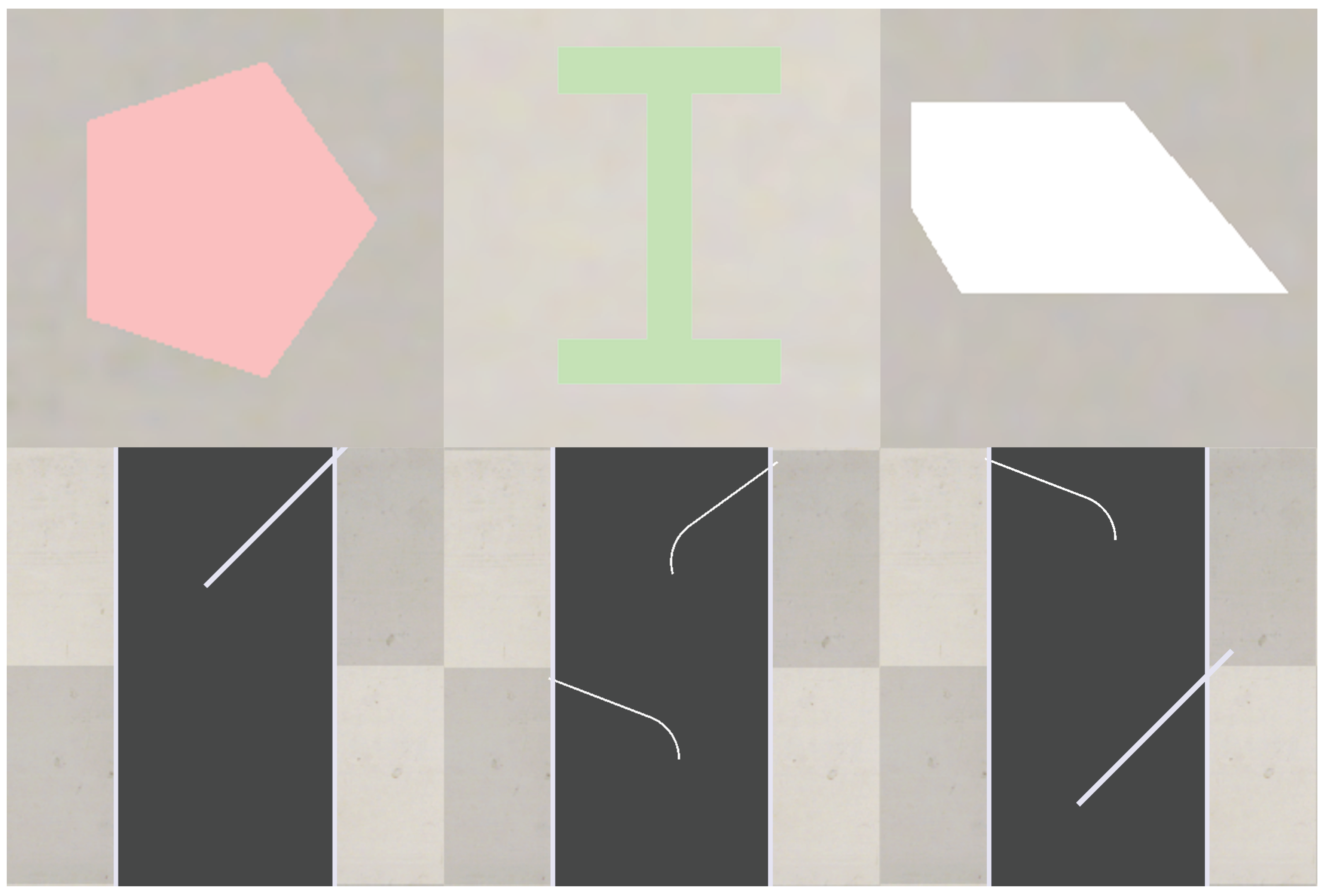
Figure 2.
Block diagram of the overall workflow illustrating the pipeline from STL import and physics simulation in CoppeliaSim to data representation using DFT, one-hot encoding, and PMF/CDF labels.
Figure 2.
Block diagram of the overall workflow illustrating the pipeline from STL import and physics simulation in CoppeliaSim to data representation using DFT, one-hot encoding, and PMF/CDF labels.
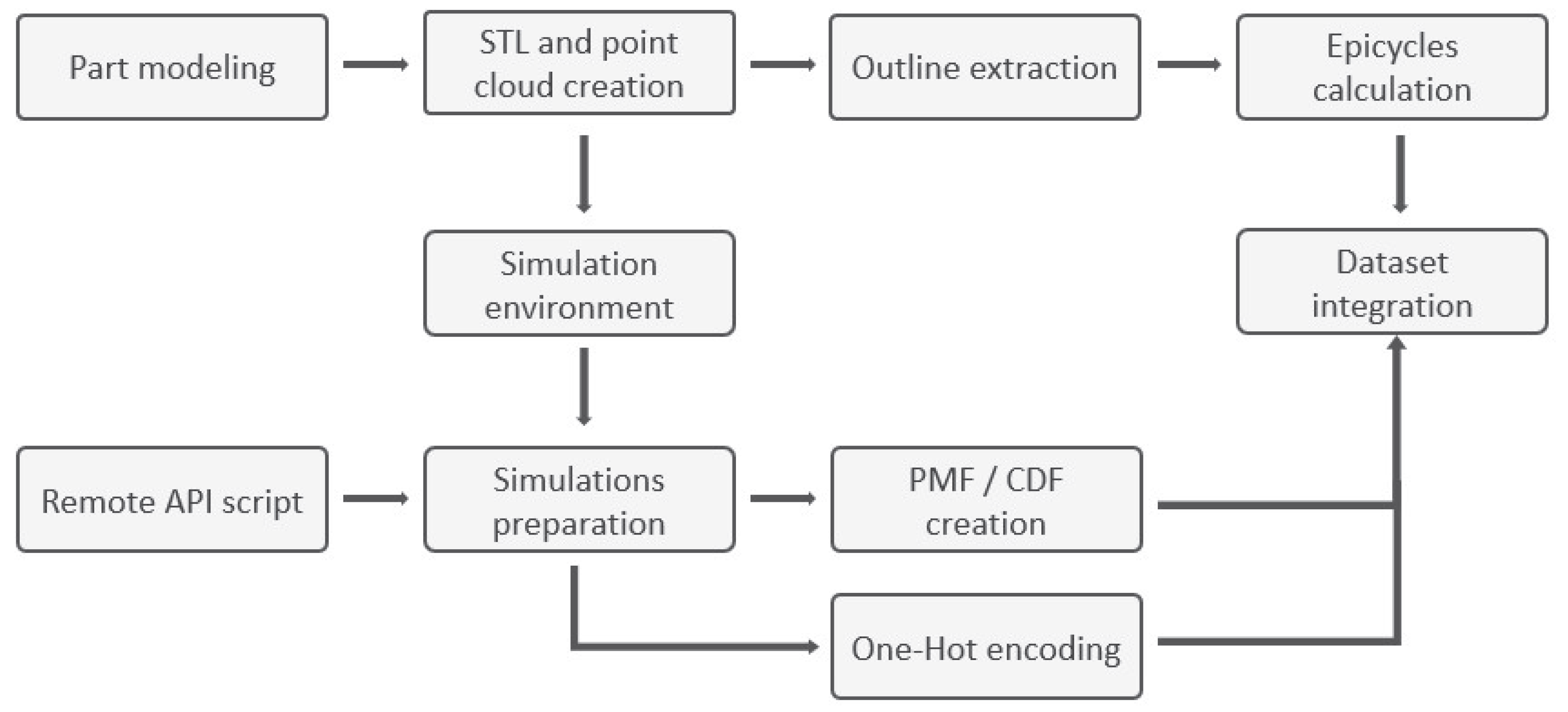
Figure 3.
Simulation overview. Panel a shows the CoppeliaSim simulation environment with a part on the linear feeder belt approaching a feeder configuration. Panel b shows time-stamped snapshots from 0 to 1800 ms of a typical simulation run, showing the part’s trajectory, fence contact, and final rest configuration. The sequence highlights stochastic elements such as initial orientation randomization and micro-impacts captured by Bullet and subsequently encoded in the orientation PMF.
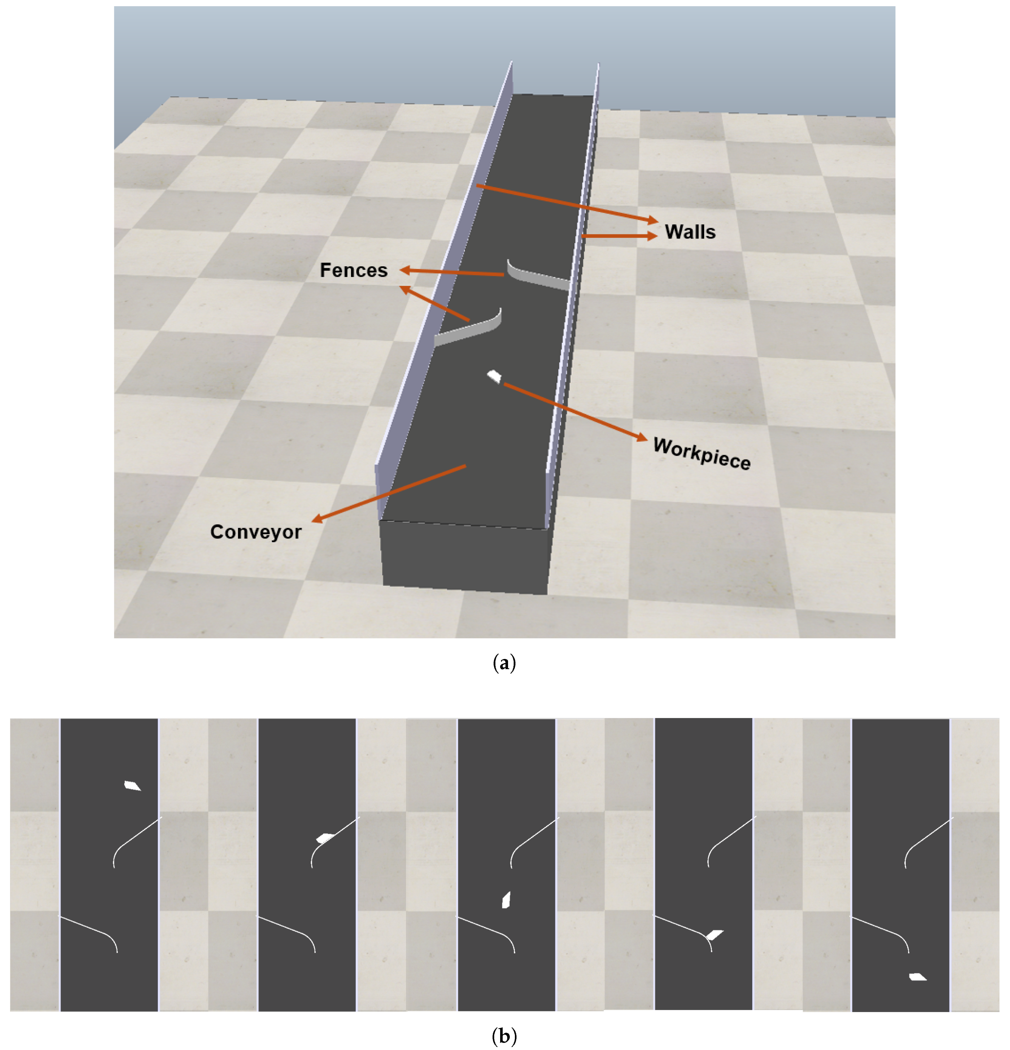
Figure 4.
Jensen–Shannon, JS, divergence between orientation distributions generated with N iterations and the full 1000-iteration reference. The curve shows mean ± SD across 10 randomly selected part–feeder configurations; see Equation 3. Note that this averaged view hides the broad distribution of JS values across all configurations.
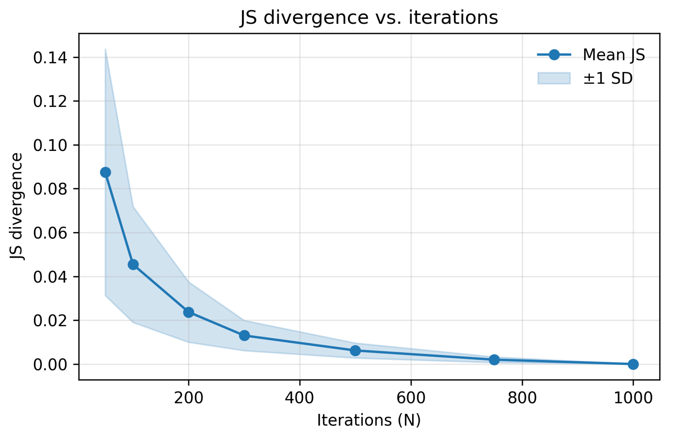
Figure 5.
Distribution of Jensen–Shannon (JS) divergence between the 100-iteration and 1000-iteration orientation PMFs across configurations. No configurations satisfy JS at 100 iterations (median JS ).
Figure 5.
Distribution of Jensen–Shannon (JS) divergence between the 100-iteration and 1000-iteration orientation PMFs across configurations. No configurations satisfy JS at 100 iterations (median JS ).
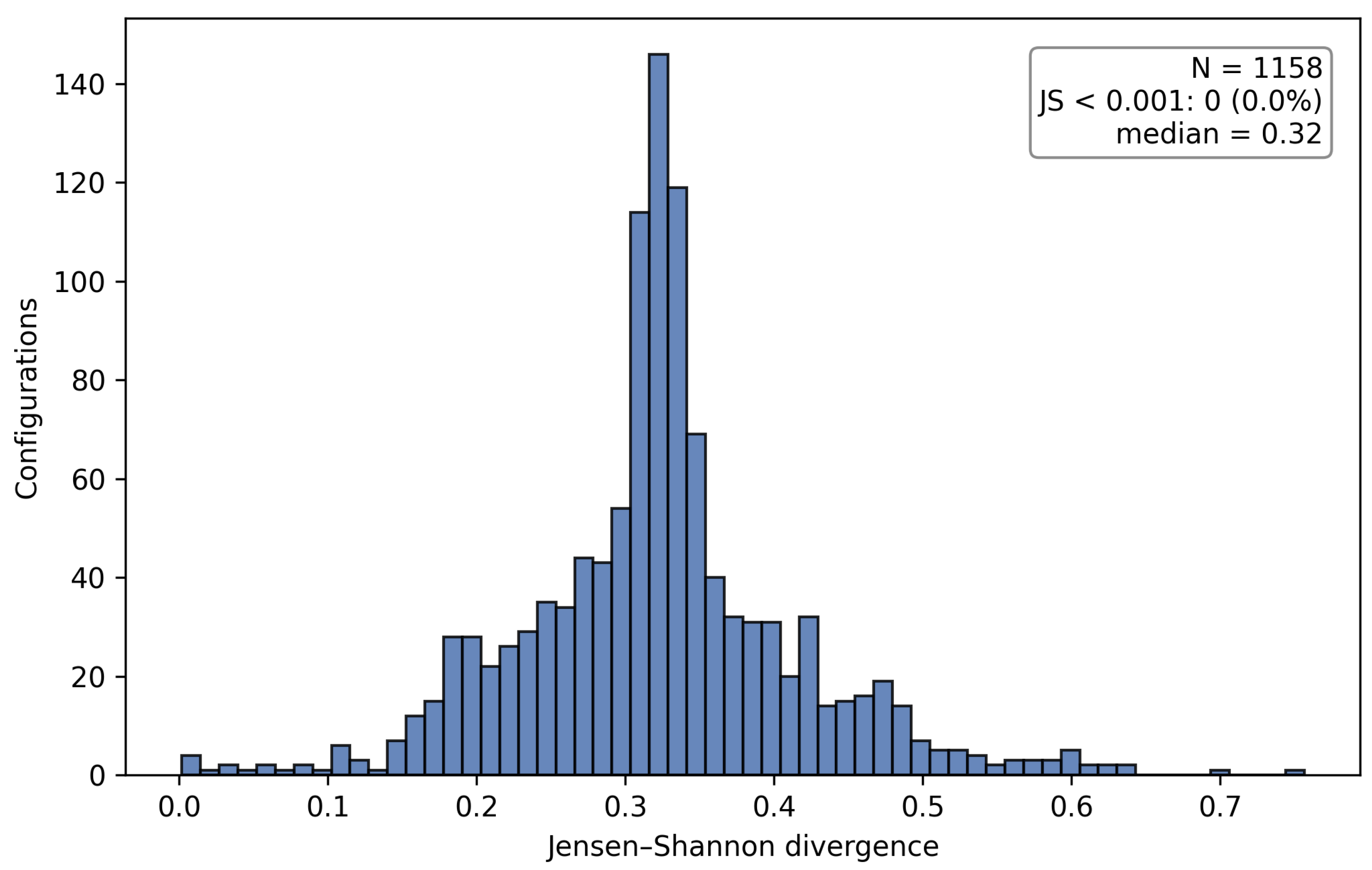
Figure 6.
DFT-based part representation. Panel a shows a conceptual illustration of representing a 2D part shape, blue outline, using a finite number of Discrete Fourier Transform coefficients, epicycles. Panel b shows examples of DFT reconstruction using 15 coefficients for diverse part shapes. Original outlines, blue, are closely approximated by the reconstructed shapes, solid orange, demonstrating the representation’s fidelity. Axes are in normalized part-coordinate units, unitless.
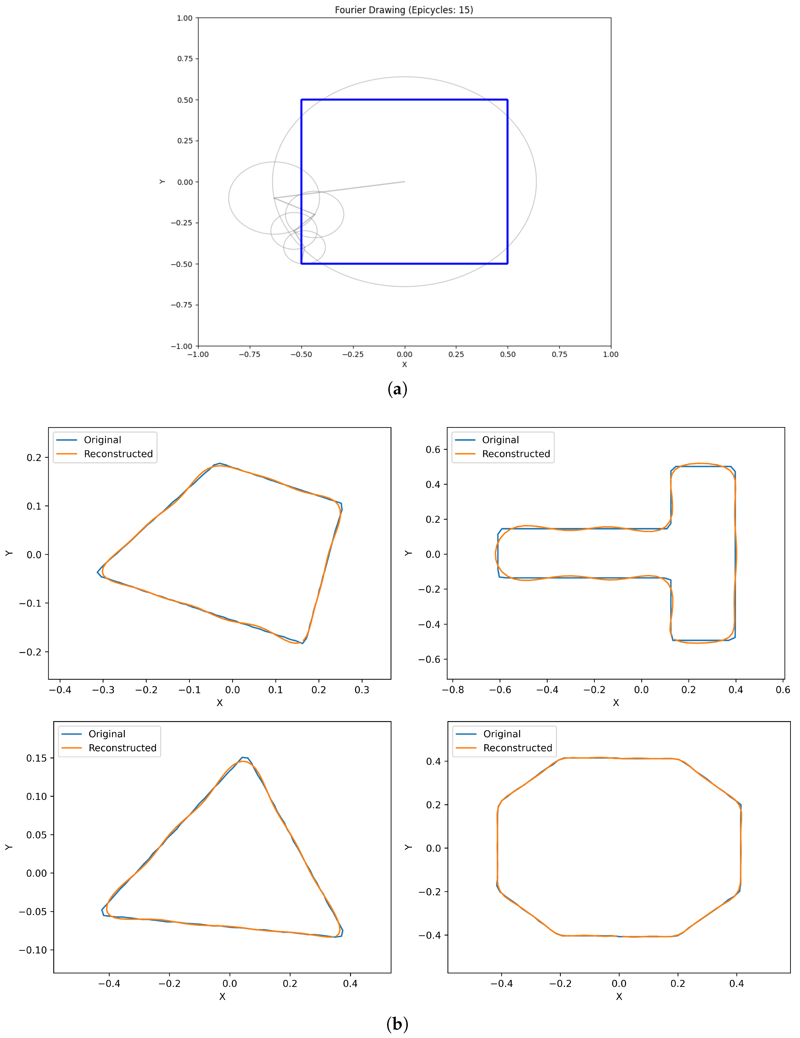
Figure 7.
Fence locations and encoding: Location 1 at m and Location 2 at m, both at m, each with lateral slots A/B at m and an outward offset to m; straight fences are rotated by angle and curved fences use radius m. The corresponding input uses one-hot encoding for fence type and presence at two locations, along with normalized angle values.
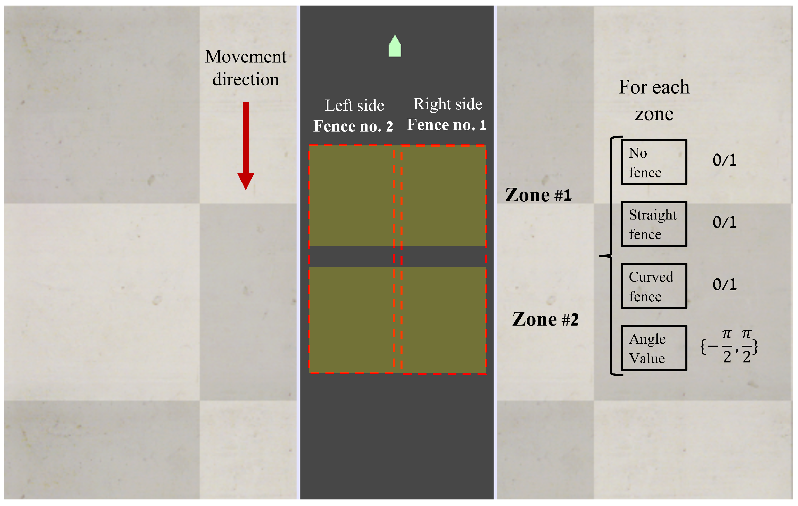
Figure 8.
Examples of fence configurations used in our dataset. Each panel shows a bird’s-eye view of a walkway (grey) with fences (white lines) on the left and/or right. The top row illustrates single-fence cases: (a) a straight fence on the right side, (b) a straight fence on the left side, (c) a curved fence on the right side, and (d) a curved fence on the left side. The bottom row shows the four possible two-fence combinations: (e) straight fences on both sides, (f) a straight fence on the right and a curved fence on the left, (g) a curved fence on the right and a straight fence on the left, and (h) curved fences on both sides. These eight scenarios cover the possible arrangements considered in the analysis.
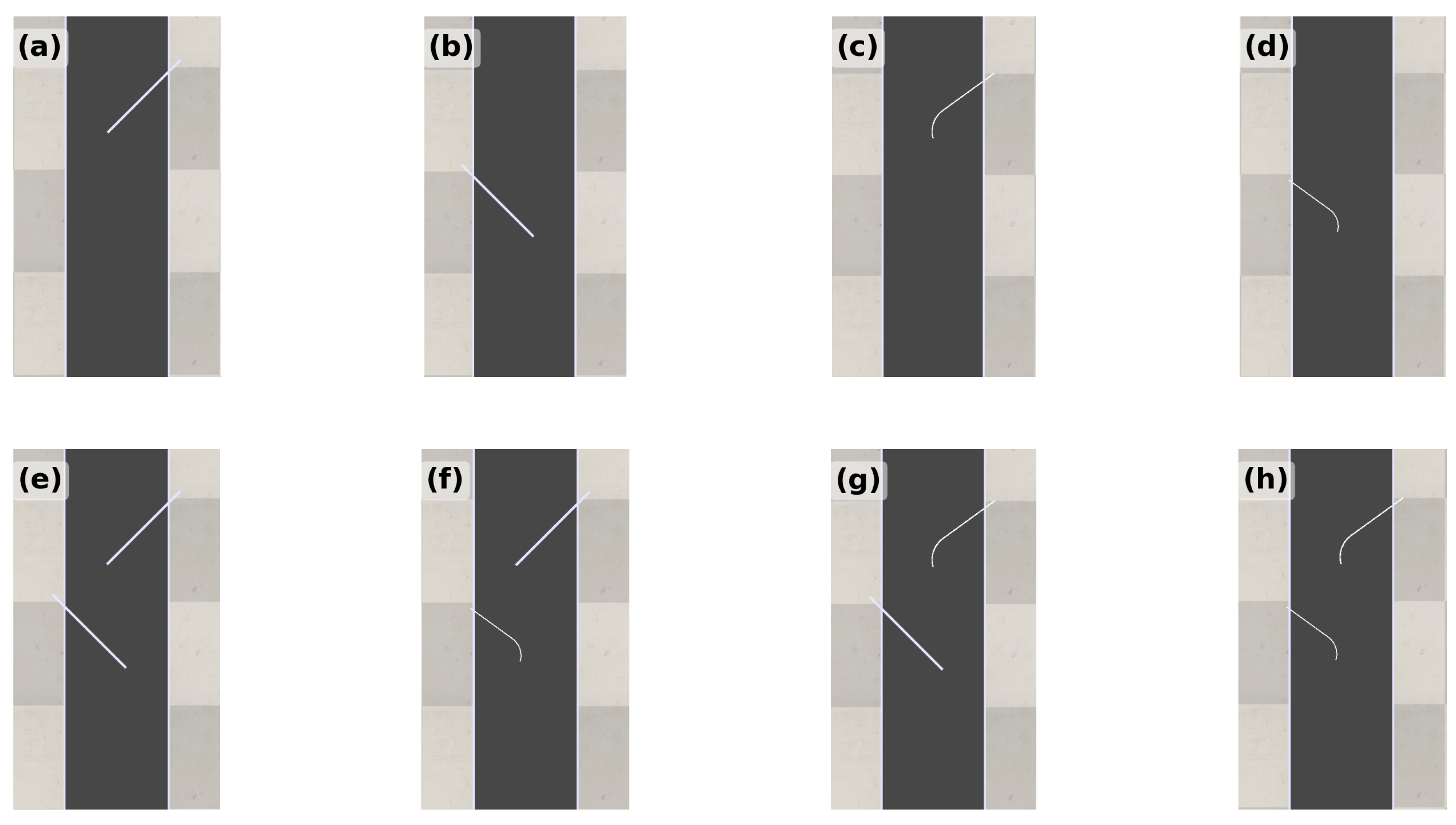
Figure 9.
Examples of final orientation distributions for different part–feeder configurations, represented as discrete PMFs with probability per bin, not CDFs. Axes: orientation angle in degrees on the x-axis and PMF, probability per bin, on the y-axis. The diversity in shapes, unimodal, multimodal, and uniform, highlights the complexity captured by the simulation data.
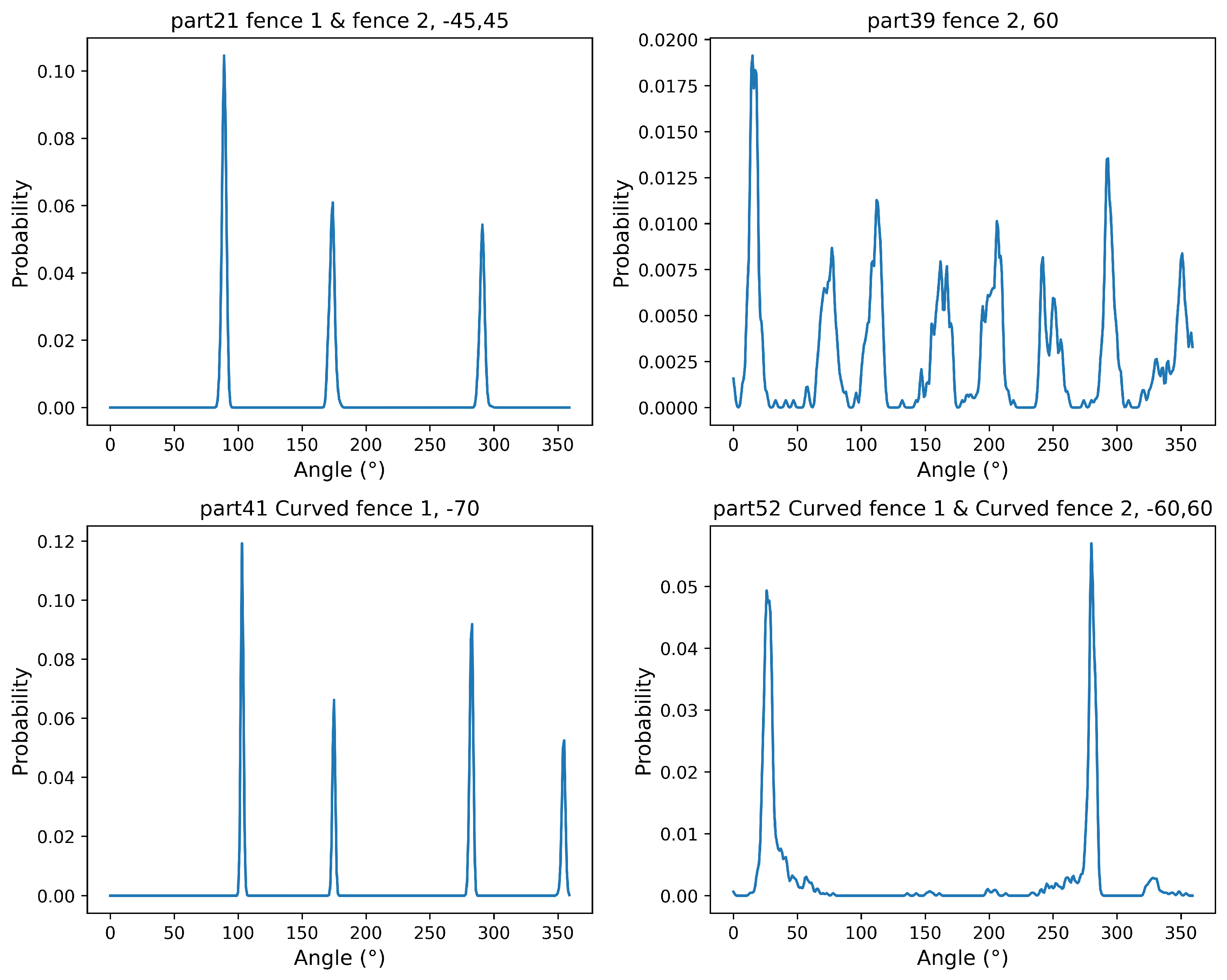
Figure 10.
Architecture of the standard fully connected regression model.
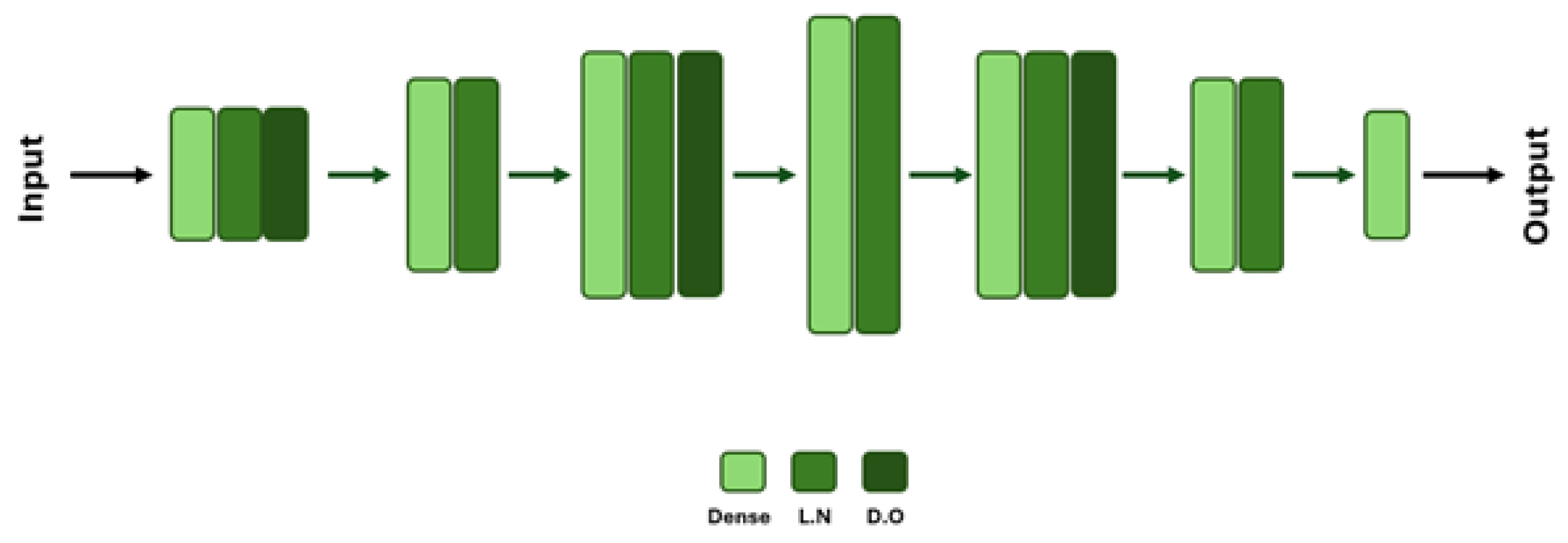
Figure 11.
VAE architecture. Part 1 is the part+feeder feature branch with 53 dimensions. Part 2 is the distribution branch with 360 CDF bins. The encoders share a latent space, and the decoder reconstructs both outputs.
Figure 11.
VAE architecture. Part 1 is the part+feeder feature branch with 53 dimensions. Part 2 is the distribution branch with 360 CDF bins. The encoders share a latent space, and the decoder reconstructs both outputs.
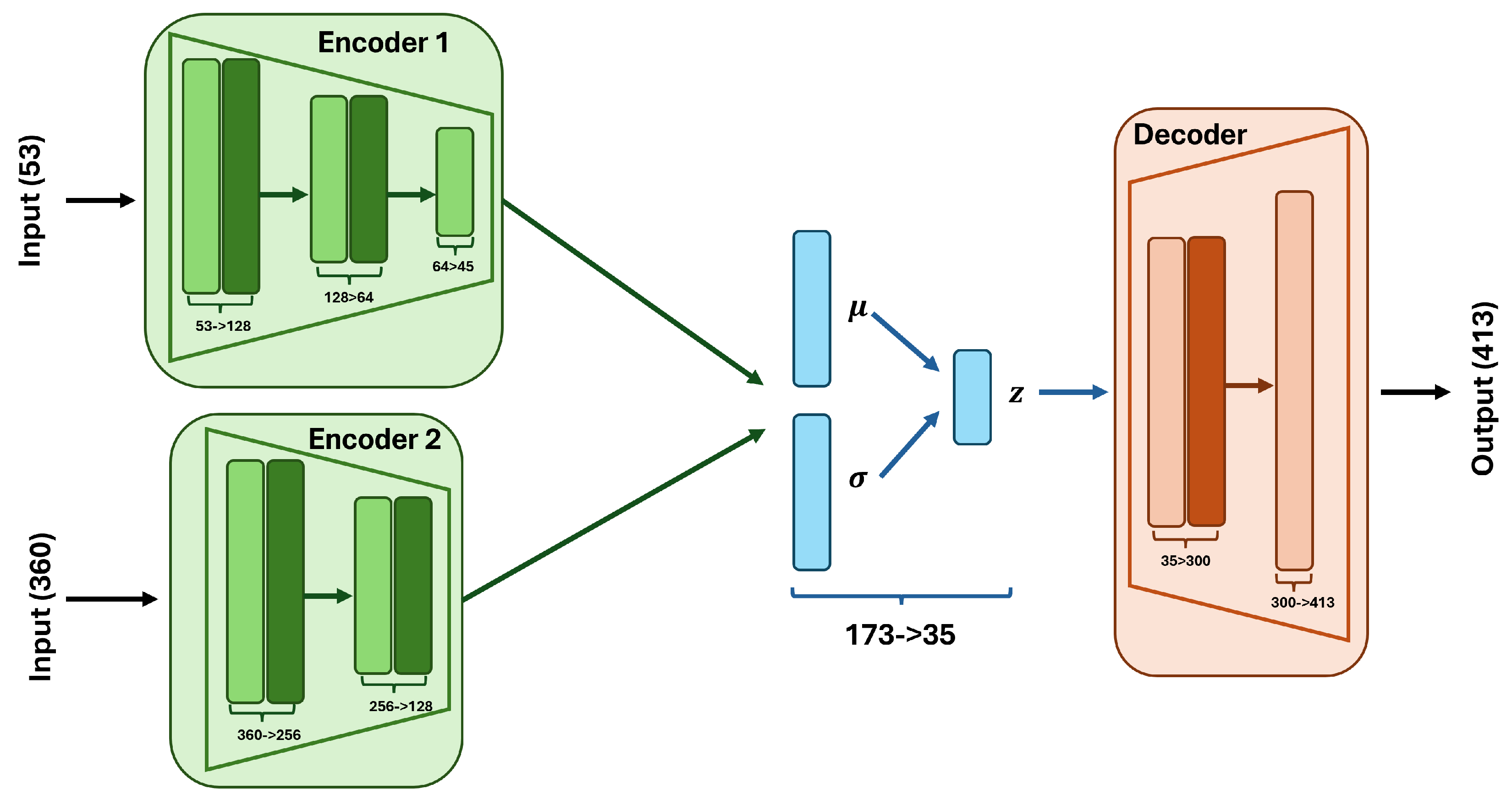
Figure 12.
Example predictions from Model 3 on the Test dataset (held-out configurations) for four representative cases, panels a–d. The model maintains good values on these held-out samples. Curves shown are circular CDFs, not PMFs, computed as unshifted cumulative sums from of the 360-bin PMF; PMFs are smoothed at dataset creation, wrapped Gaussian with , and no shared shift is applied. Model 3 outputs PMFs, and we plot their derived CDFs. Axes: orientation angle in degrees on the x-axis and CDF, unitless cumulative probability, on the y-axis.
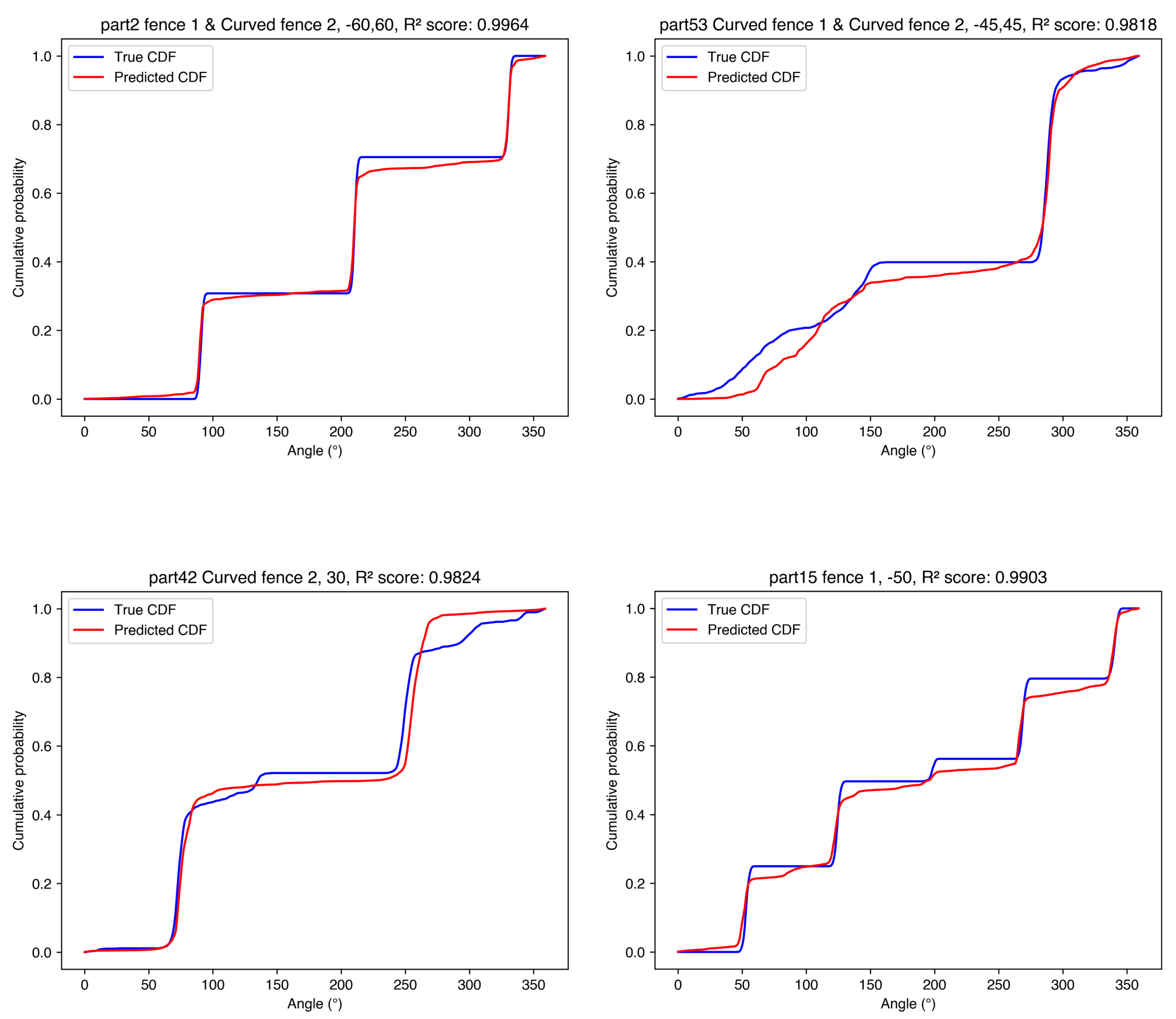
Figure 13.
Example predictions from Model 3 on the Parts dataset with unseen part geometries and only 3 unique parts for four representative cases. The significant performance drop highlights the difficulty of generalizing to new shapes. Curves shown are circular CDFs, not PMFs, computed as unshifted cumulative sums from of the 360-bin PMF; PMFs are smoothed at dataset creation, wrapped Gaussian with , and no shared shift is applied. Model 3 outputs PMFs, and we plot their derived CDFs. Axes: orientation angle in degrees on the x-axis and CDF, unitless cumulative probability, on the y-axis.
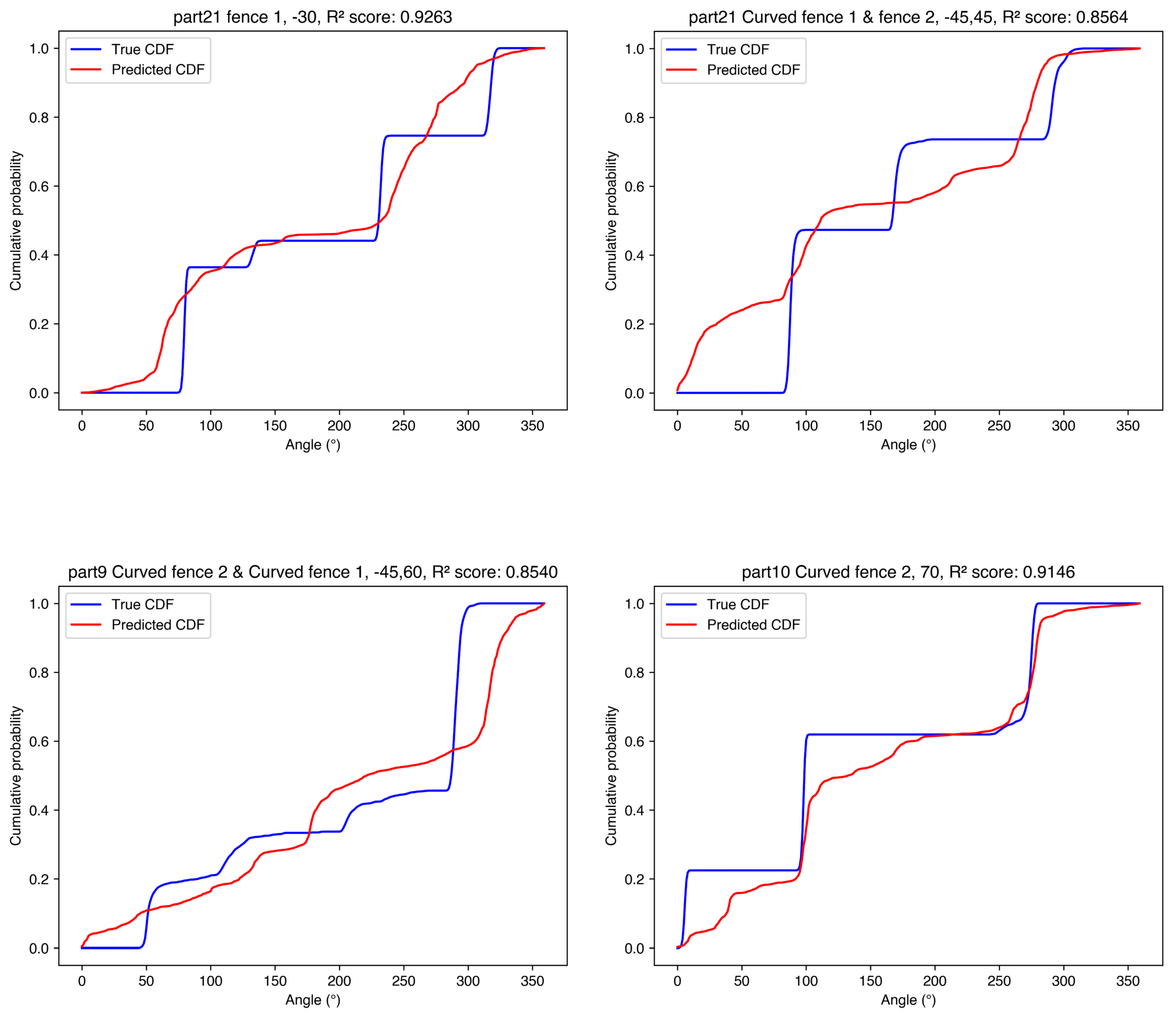
Figure 14.
Cross-convergence evaluation comparing within-level reconstruction (green, control) against partial-to-100% prediction (red). The within-level curve shows stable across all iteration levels, confirming the VAE architecture is sound. The cross-convergence curve shows that predicting fully converged CDFs from partial-iteration inputs yields poor results () at fewer than 30 iterations, with substantial improvement only above 60–70%. Error bars show ±1 SD across holdout configurations. This demonstrates that partial simulations lack sufficient information to predict final distributions until convergence is nearly complete.
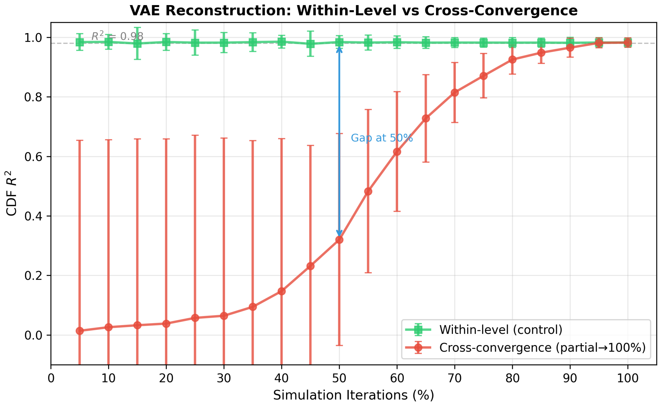

Table 1.
Key Simulation and Data Processing Parameters.
| Parameter | Value | Units/Notes |
|---|---|---|
| Simulator | CoppeliaSim Edu 4.6 | Platform [28] |
| Physics engine | Bullet 2.78 | Timestep 5 ms; 10 substeps [29] |
| Gravity | Not explicitly set | Scene default; not logged in API script |
| Contact solver iterations | Not explicitly set | Scene default; not logged |
| ERP/CFM | Not explicitly set | Engine defaults; not logged |
| Linear/angular damping | Not explicitly set | Scene defaults; not logged |
| Friction combine mode | Not explicitly set | Engine default; not logged |
| Restitution combine mode | Not explicitly set | Engine default; not logged |
| Conveyor speed | 0.10 | m/s; chosen for stable transport and fence interaction in simulation; not calibrated to a specific feeder |
| Friction coefficients (Coulomb ) | Parts 0.8; fences 0.5; belt 1.0 | Static = kinetic; effective parameters for stable, friction-dominated motion; not calibrated [29] |
| Restitution coefficients | Highly damped contacts to reduce bounce in Bullet [29] | |
| Initial part orientation () | (, , ) | Flat on belt, random yaw |
| Simulation iterations per config. | 1000 | Chosen based on JS divergence analysis (Figure 4) |
| Output angle range | Degrees (simulator-native) | |
| PMF smoothing | Wrapped Gaussian | Circular convolution; |
| Part representation | DFT | 15 largest coefficients (freq, mag, phase) |
| Feature vector (part) | 45 | Standardized parameters (z-score) |
| Feeder representation | 8 | 2x [3 one-hot type + 1 scalar angle min–max scaled to on training split; angle set to 0 when type=None] |
| Fence geometry (straight) | Fixed | Rigid cuboid; dimensions fixed in CoppeliaSim scene (length/width/thickness not varied; values not logged) |
| Fence geometry (curved) | Arc segment with fixed cross-section (length/width/thickness fixed in scene; values not logged); placement uses radius r | |
| Fence placement slots | ; ; | Locations 1/2 (downstream/upstream) and lateral A/B offsets |
| Conveyor implementation | CoppeliaSim Conveyor model | Built-in conveyor object with constant belt velocity; internal parameters not logged |
| Label representation (options) | Full (360)PCA (170/85) | Bin counts for PMF/CDF: PMF 360 or 170; CDF 360 or 85 |
Table 2.
Summary of Designed Regression Models
| Model | Label Type | Label Repr. | Architecture | Loss Function Notes |
|---|---|---|---|---|
| 1 | PMF | PCA (170) | Standard FC | MSE |
| 2 | PMF | PCA (170) | Branched FC | MSE |
| 3 | PMF | Full (360) | Standard FC | MSE (CDF)+ KL (PMF)+ KS (CDF) |
| 4 | PMF | Full (360) | Branched FC | MSE (CDF)+ KL (PMF)+ KS (CDF) |
| 5 | CDF | PCA (85) | Standard FC | MSE (PMF)+ MSE (CDF) |
| 6 | CDF | PCA (85) | Branched FC | MSE (CDF) |
| 7 | CDF | Full (360) | Standard FC | MSE (PMF)+ KS (CDF) |
| 8 | CDF | Full (360) | Branched FC | MSE (PMF)+ KS (CDF) |
Table 3.
VAE Hyperparameters, CDF reconstruction
| Parameter | Value |
|---|---|
| Latent Dimension | 35 |
| Learning Rate | 0.002 |
| Batch Size | 64 |
| Epochs | 120 |
| Optimizer | Adam, weight decay 3e-5 |
| Gradient Clipping | Max norm: 5.0 |
| Loss Weights: recon P+C, recon CDF, KL, KS penalty | 2, 8, 0.25, 20 |
| Gradient penalty weight, | 4 |
| KL Annealing Schedule | Weight grew linearly, capped at 0.25 |
Table 4.
Dataset Summary, total samples = 1,236.
| Dataset | Samples | Unique Parts | Purpose | Protocol |
|---|---|---|---|---|
| Main (Train) | 890 | 38 | Model training | – |
| Main (Test) | 158 | 38 | Held-out configurations (random split) | P1 |
| Fences | 78 | 18 | Unseen fence configurations | P1 |
| Parts | 110 | 3 | Unseen part geometries | P3 |
| Total (All) | 1,236 | 41 | All datasets combined | – |
Table 5.
Regression Model Performance on Training Data: and in deg, mean ± SD; configurations.
| Model | [deg] | |
|---|---|---|
| Model 1 | ||
| Model 2 | ||
| Model 3 | ||
| Model 4 | ||
| Model 5 | ||
| Model 6 | ||
| Model 7 | ||
| Model 8 |
Table 6.
Regression Model Performance on Test Dataset: and in deg, mean ± SD; configurations.
| Model | [deg] | |
|---|---|---|
| Model 1 | ||
| Model 2 | ||
| Model 3 | ||
| Model 4 | ||
| Model 5 | ||
| Model 6 | ||
| Model 7 | ||
| Model 8 |
Table 7.
Regression Model Performance on Fences Dataset, unseen feeder configurations: and in degrees, mean ± SD; configurations.
Table 7.
Regression Model Performance on Fences Dataset, unseen feeder configurations: and in degrees, mean ± SD; configurations.
| Model | [deg] | |
|---|---|---|
| Model 1 | ||
| Model 2 | ||
| Model 3 | ||
| Model 4 | ||
| Model 5 | ||
| Model 6 | ||
| Model 7 | ||
| Model 8 |
Table 8.
Regression Model Performance on Parts Dataset: and in deg, mean ± SD; configurations.
| Model | [deg] | |
|---|---|---|
| Model 1 | ||
| Model 2 | ||
| Model 3 | ||
| Model 4 | ||
| Model 5 | ||
| Model 6 | ||
| Model 7 | ||
| Model 8 |
Table 9.
VAE Reconstruction Performance, mean ± SD, unitless, on held-out Fences, , and Parts, , datasets. The VAE was trained only on the Main dataset, ; Fences and Parts were excluded from training. This table reports autoencoding reconstruction accuracy using both part+feeder features and CDF inputs, not conditional prediction from geometry alone.
| Dataset | (Part+Feeder) | (CDF) |
|---|---|---|
| Fences | ||
| Parts |
Table 10.
Delta-to-full correction performance (CDF ) at representative iteration levels. Cost saved is . Part split = unseen parts; config split = random configuration split with parts seen during training. Full 5% sweep results are provided in Supplementary Section S11.
Table 10.
Delta-to-full correction performance (CDF ) at representative iteration levels. Cost saved is . Part split = unseen parts; config split = random configuration split with parts seen during training. Full 5% sweep results are provided in Supplementary Section S11.
| Level | Cost saved (%) | Part split () | Part baseline | Config split () | Config baseline |
|---|---|---|---|---|---|
| 5% | 95.0 | 0.82±0.22 | -0.02±0.69 | 0.83±0.21 | -0.02±0.69 |
| 10% | 90.0 | 0.82±0.21 | -0.01±0.68 | 0.83±0.21 | -0.01±0.69 |
| 25% | 75.0 | 0.84±0.18 | 0.03±0.62 | 0.84±0.20 | 0.03±0.62 |
| 50% | 50.0 | 0.86±0.16 | 0.31±0.35 | 0.86±0.18 | 0.31±0.36 |
| 75% | 25.0 | 0.96±0.07 | 0.89±0.06 | 0.95±0.06 | 0.89±0.06 |
| 90% | 10.0 | 0.99±0.01 | 0.99±0.01 | 0.99±0.01 | 0.99±0.01 |
Disclaimer/Publisher’s Note: The statements, opinions and data contained in all publications are solely those of the individual author(s) and contributor(s) and not of MDPI and/or the editor(s). MDPI and/or the editor(s) disclaim responsibility for any injury to people or property resulting from any ideas, methods, instructions or products referred to in the content. |
© 2026 by the authors. Licensee MDPI, Basel, Switzerland. This article is an open access article distributed under the terms and conditions of the Creative Commons Attribution (CC BY) license (http://creativecommons.org/licenses/by/4.0/).
Copyright: This open access article is published under a Creative Commons CC BY 4.0 license, which permit the free download, distribution, and reuse, provided that the author and preprint are cited in any reuse.


