
Submitted:
13 September 2024
Posted:
13 September 2024
You are already at the latest version
Abstract
(1) Background: Efficient detection and rectification of defects or post-processing manufacturing conditions such as sharp edges and burrs on metal components are crucial for quality control in precision manufacturing industries. (2) Methods: This paper describes a lab-scale integrated system for real-time and automated metal edge image detection using a customized YOLOv5 ma-chine vision algorithm. The YOLOv5 algorithm and model were developed and embedded in the NVIDIA Jetson Nano microprocessor. The YOLOv5 model can detect three different image types for classification i.e., normal, sharp, and burrs edge on aluminum workpiece blocks. An integrated system connects the NVIDIA Jetson Nano with an embedded YOLOv5 model to a Mitsubishi Electric Melfa RV-2F-1D1-S15 manipulator to perform selective automated chamfer-ing and grinding when certain condition defects are detected. (3) Results: The model demonstrates durable performance, achieving a mean average precision of 0.886 across defect classes with minimal misclassifications. The Mitsubishi Electric Melfa RV-2F-1D1-S15 manipulator received input from the machine vision system and performed an automated chamfering and grinding process accordingly; (4) Conclusions: By integrating camera, embedded deep learning in the microprocessor and manipulator, automated chamfering and grinding process in metal component shapes can be efficiently rectified. This tailored solution promises to improve productivity and consistency in metal manufacturing and remanufacturing.
Keywords:
automated chamfering and grinding
; deep learning
; intelligent manufacturing and remanufacturing
; machine vision
; robotic manufacturing
1. Introduction
The manufacturing industry has experienced a major transformation in recent years. The increasing need for automation has driven the manufacturing industry. Implementing automation in manufacturing enhances the efficiency and precision of the process as well as improves quality control [1]. As industries maintain product consistent quality, the inconsistent shape issue during the manufacturing process needs to be solved. Psarommatis et al. [2] present a literature review study on the methods to minimize product defects in industrial production lines based on 280 articles published from 1987 to 2018. The study identified four strategies: detection, repair, prediction, and prevention. The essence revolves around the depreciation of deficiencies within the end product and across its components and the energy consumption in the production process, among many other indicators [3]. Detection was the most commonly used strategy, followed by quality assessment after the product was fully fabricated.
In decades, manufacturing has transformed from digital to intelligent manufacturing [4]. The paper categorized the manufacturing transformation into i.e., digital manufacturing, digital-networked manufacturing, and new-generation intelligent manufacturing. It emphasizes integrating new-generation AI technology with advanced manufacturing technology as the core driving force of the new industrial revolution. The paper also introduces the concept of Human-Cyber-Physical Systems (HCPS) as the leading technology in intelligent manufacturing.
Artificial Intelligence (AI) improves conventional methods by enabling consistent, effective, efficient, and reliable processes and the end product. This is because a human-dependent manufacturing process typically faces problems such as inconsistency, inaccuracy due to human error, human fatigue, and the absence of an expert. Such issues can be solved by incorporating AI, especially Machine Learning (ML) and Deep Learning (DL) methods [5]. One of the particular important process in the manufacturing process is the grinding and chamfering. These method are included in the surface finishing process to enhance the product quality. The automation process for grinding and chamfering tasks is becoming more significant due to requirements for exactness and efficiency. Systems for grinding and polishing driven by robots with have visual recognition abilities will increase an accuracy while significantly reduce the time taken for manual work. Adding machine learning into these kinds of processes makes possible adjustments in real-time. This optimizes how things are done because it keeps track of when the wheel used for grinding needs dressing, so performance is improved, and waste is lessened. For an automated grinding and chamfering processes with a machine vision based AI has a main task to detect the edge to be processed by grinding and chamfering. An examples of the edge detection using non-AI and AI methods are presented in the following paragraphs:
An example application of image processing method based on wavelet transform for edge detection is presented in [6]. The paper presents an image edge detection algorithm that utilizes multi-sensor data fusion to enhance defect detection in metal components. The edge detection accuracy of the method is improved by integrating data from ultrasonic, eddy current, and magnetic flux leakage sensors using wavelet transform. It is also demonstrated that the result of the proposed method with fused-sensor data outperforms single-sensor data [6].
An example application of AI (Machine Learning) for edge detection is presented in [7]. Yang et al. [7] used Support Vector Machine (SVM) to identify defects in logistics packaging boxes. The authors developed an image acquisition protocol and a strategy to address the defects commonly found in packaging boxes used in logistics settings. The first phases required constructing a denoising template and utilizing Laplace sharpening methods to improve the picture quality of packaging boxes. Next, they used an enhanced morphological approach and an algorithm based on grey morphological edge detection to eliminate noise from box pictures. The study finished with extracting and transforming packing box characteristics for quality classification utilizing the scale-invariant feature transform technique and SVM classifiers. The results indicated a 91.2% likelihood of successfully detecting two major defect categories in logistics packing boxes: surface and edge faults. Although the SVM method performed satisfactorily in the edge detection and classification, it required a denoising, a sharpening, and a feature extraction method which are not applicable and unreliable for the software to hardware implementation and deployment.
An example application of AI (Deep Learning) for edge detection is presented in [8] and [9] [10]. The Canny-Net neural network adaption of the classic Canny edge detector is presented in [8]. It is intended to solve frequent artifacts in CT scans, including scatter, complete absorption, and beam hardening, especially when metal components are present. Comparing Canny-Net to the traditional Canny edge detector, test images show an 11% rise in F1 score, indicating a considerable performance improvement. Notably, the network is computationally efficient and versatile for a range of applications due to its lightweight design and minimal set of trainable parameters. A study presented in [9] contributes a new approach that would help identify the mechanical defects in high voltage circuit breakers through integrating advanced edge detection with DL. Circuit breakers with higher resolution images undergo through contour detection, binarization and morphological processing. These images are then processed for feature extraction and for the identification of defects in the product through a DL platform on TensorFlow and Convolutional Neural Network (CNN). It is shown that this method is more accurate and has better feature extraction than classical CNN models for defect detection including plastic deformation, metal loss, and corrosion. This method ensures a safe method of identifying mechanical faults without destroying the High voltage circuit breaker and improve maintenance, and thus minimize failure. The convolution method in deep learning is particularly effective and prevalent in edge detection; its integration with various techniques, such as lighting adjustments or horizontal and vertical augmentation, yields substantial results [10]. The implementation of machine vision in the experiments by González et al. for edge detection and deburring significantly enhanced chamfer quality with precision and efficiency [11].
Robot manipulators has been useful in manufacturing processes as they are excellent at performing multiple tasks and completing them. Recent advancements in combining DL with robot manipulators have opened a new research direction and potential application in practice. Studies in this area have gained much attention to elaborate on robot manipulator performance in the application of intelligent manufacturing. The use of deep reinforcement learning algorithms has been integrated into robot manufacturing and has shown a good result in helping robot manipulators for grasping and object manipulation [12]. It shows how manipulators grasp, handle, and manipulate better with relatively less time [12]. Using advanced algorithms from deep reinforcement learning, experts have made the work of robot manipulators better in terms of their speed to adapt, accuracy, and overall performance. This progress opens possibilities for creating smarter and more effective robots in future research [13] [14] [15]. Furthermore, algorithms have been made to control robot manipulators with vision through deep reinforcement learning. They help robots pick up the objects by themselves based on the visuals and demonstrate how incorporating DL can improve the work of handling things during the robot’s movement and performance [16].
YOLOv5 is a powerful tool for image recognition and object detection [17]. Aein et al. [18] devised a technique to assess the integrity of metal surfaces. The authors employed the YOLO object detection network to detect faults on metal surfaces, resulting in an integrated inspection system that can distinguish between different types of defects and identify them immediately. The solution was implemented and evaluated on a Jetson Nano platform with a dataset from Northeastern University. The investigation yielded a mean Average Precision (mAP) of 71% across six different fault types, with a processing rate of 29 FPS.
Li et al. [19] employed the YOLO algorithm to create a method for real-time identification of surface flaws in steel strips. The authors improved the YOLO network, making it completely convolutional. Their unique approach offers an end-to-end solution for detecting steel-strip surface flaws. The network obtained a 99% detection rate at 83 frames per second (FPS). The invention also involves anticipating the size and location of faulty zones. The YOLO network was upgraded by creating a convolutional structure with 27 layers. The first 25 levels gather useful information about surface defect features on steel strips, while the final two layers forecast defect types and bounding boxes.
Xu et al. [20] developed a novel modification of the YOLO network to enhance metal surface flaw identification. Their strategy centred on creating a new scale feature layer to extract subtle features associated with tiny flaws on metal surfaces. This invention combined Darknet-53 architecture’s 11th layer with deep neural network characteristics. The k-means++ technique significantly lowered the sensitivity of the first cluster. The study yielded an average detection performance of 75.1% and a processing speed of 83 frames per second.
A number of study has reported a benefit of YOLO on the hardware implementation using NVIDIA Jetson Nano [21], [22]. The NVIDIA Jetson Nano, notable for its computational capabilities, facilities the infusion of AI models into devices [23]. The NVIDIA Jetson Nano is a device which have a low power consumption and can performs real-time inferences that can be considered in terms of frame rates. For instance, the implementations of YOLOv3-tiny show that the system-level approaches can achieve frame rates of approximately 30 FPS, which is crucial for surveillance and monitoring purposes [24], [25]. The YOLO algorithm and architecture has a benefit in the application of object detection in machine vision i.e., the determination of objects on images can be done in a single pass, which helps to reduce the amount of computational work several times compared with multi-step methods [26]. This results in high efficiency, particularly when it is deployed on the NVIDIA Jetson Nano, which, due to its insufficient power compared to other Graphics Processing Units (GPUs), can handle satisfactory performance with optimized models [27].
Integrating robot manipulators with machine vision technologies has revolutionized various industrial applications [28]. In certain industries, automatic manufacturing with machine vision technologies can reduce workers’ risks while performing repetitive and potentially hazardous tasks [29]. A method presented using the YOLO Convolutional Neural Network for analyzing video streams from a camera on the robotic arm, recognizing objects, and allowing the user to interact with them through Human Machine Interaction (HMI), which helps the movement of individuals with disabilities [30]. The method involves using the Niryo-One robotic arm equipped with a USB HD camera and modifying the YOLO algorithm to enhance its functionality for robotic applications, showing that the robotic arm can detect and deliver objects with high accuracy and in a timely manner [31]. The study suggests an industrial simulation, a practical robotic application using robot manipulators and DL to perform both grinding and chamfering simultaneously. The approach of incorporating robotic manipulators and computer vision systems based on DL to carry out grinding and chamfering tasks automatically is an essential aspect of this research. This study utilizes the capabilities of a robot manipulator, specifically, the Mitsubishi Electric Melfa RV-2F-1D1-S15 to execute precise grinding and chamfering tasks in the lab experimental study. This study aims to proof that the machine vision technology can be integrate with the robot manipulator because it is expected that by integrating manipulator and computer vision technology it can increase the precision and efficiency of the grinding and chamfering process.

Table 1.
Acronyms and abbreviations.
| Acronym | Abbreviation |
|---|---|
| AI | Artificial intelligence |
| AP | Average Precision |
| AUC | Area Under the Curve |
| CAD | Computer Aided Design |
| CM | Confusion Matrix |
| CNN | Convolutional Neural Network |
| COCO | Common Objects in COntext |
| CSPNet | Cross-Stage Partial Network |
| CT | Computed Tomography |
| CVAT | Computer Vision Annotation Tools |
| DL | Deep Learning |
| DOF | Degree of Freedom |
| F1 | Precision-recall score |
| FLOPS | Floating-point Operations Per Second |
| FPS | Frames per second |
| FPN | Feature Pyramid Networks |
| FN | False Negative |
| FP | False Positive |
| GPU | Graphics Processing Unit |
| HCPS | Human-Cyber-Physical Systems |
| HMI | Human Machine Interaction |
| IoU | Intersection over Union |
| mAP | Mean Average Precision |
| ML | Machine Learning |
| PANet | Pyramid Aggregation Network |
| ROC | Receiver Operating Characteristic |
| RPN | Region Proposal Network |
| SGD | Stochastic Gradient Descent |
| SPP | Spatial Pyramid Pooling |
| SSD | Single Shot Detector |
| SVM | Support Vector Machine |
| TN | True Negative |
| TP | True Positive |
| VGG | Visual Geometric Group |
| VOC | Visual Object Classes |
2. Machine Vision based Deep Learning Algorithm
2.1. Deep Learning Algorithm (VGG16, YOLOv5, YOLOv8)
2.1.1. VGG
The VGG16 network architecture has 16 layers comprising 13 convolutional layers and 3 fully connected layers. This network includes a 3x3 small filter with a stride of 1 convolutional operation while it includes a max pooling layer of 2x2 windows and a stride after every two convolutional layers [32]. VGG-16 is applied to classify six surface defects on steel strips [33]. The image data was from the NEU image dataset. VGG’s architecture is presented in Figure 1.
2.1.2. YOLOv5
YOLO detection object family is a common approach for object detection [34], expanding on the improvements achieved in its family, YOLOv1 through YOLOv8. Its performance has been constantly improved by comparing its skills against two well-known object identification datasets: Pascal VOC (visual object classes) and Microsoft COCO (common objects in context). The model is built on a convolutional neural network system with four components, as presented in Figure 2. The framework includes four major components that are (1) a backbone module for extracting features, (2) a neck module that integrates multiple-level features, such as feature pyramid networks (FPN), (3) a Region Proposal Network (RPN) to create region proposals which is only applicable to two-stage detectors, and (4) the head module provides the final classification and localization results [35]. The YOLOv5 model is based on the CSPDarknet53 architecture and has a spatial pyramid pooling (SPP) layer. Furthermore, PANet is used as the neck component, while YOLO detection is used as the head component.
The YOLOv5 model employs the CSPDarknet architecture, which includes the cross-stage partial network (CSPNet) within the Darknet framework. This backbone network enhances the model’s capacity to extract features while also increasing its depth. The CSPNet design decreases the amount of parameters and floating-point operations per second (FLOPS), allowing for quicker and more accurate inference and a smaller model size. The neck network incorporates a route aggregation network (PANet) to alleviate the issue of restricted propagation of low-level features in the original feature pyramid networks. PANet uses accurate localization signals in lower layers to increase the precision of object localization [36]. The Head network in both YOLOv3 and YOLOv5 architectures comprises three major components: bounding box loss, categorization loss, and confidence loss. The loss function for the classification and confidence losses is binary cross-entropy, while the loss function for the bounding box loss is intersection over union (IoU) loss [37]. The YOLOv5 framework consists of five models: YOLOv5s, YOLOv5m, YOLOv5l, YOLOv5n, and YOLOv5x. YOLOv5s was chosen for this project because of its small size and fast processing speed, making it the most suitable model. The Ultralytics team has made the model public on GitHub. The model is built up with pre-trained weights from the COCO dataset [38].
2.1.3. ResNet (Residual Network)
ResNet, or Residual Network, is a deep learning architecture that was introduced by He et.al., in 2016 [39]. ResNet’s has impressive ability to efficiently solve the degradation problem in deep neural networks. The ResNet mechanism skips connections in residual blocks to address the vanishing gradient problem. These connections allow ResNet to learn the residual function based on the input layer and enable the network to train much deeper than previously [40]. The ResNet architecture is presented in Figure 3.
2.2. Performance Evaluation
In machine vision technology, an accurate prediction is essential for assessing an object identification system’s efficacy. Object detection models have a dual objective, which involves localising and classifying objects. As a consequence, the total performance of the model is evaluated by taking into account the outcomes of both tasks. The representation of object detection includes three primary attributes: the item’s categorization or labelling, the defining of its bounding box, and the quantification of the confidence score. A confidence score is a numerical number ranging from 0 to 1 that indicates the degree of certainty the model has in its prediction.
The accuracy of the prediction is determined by comparing the detected bounding box and the label assigned during annotation with the actual bounding box. This section describes how the model is assessed using several performance measures based on the ground-truth bounding box and label data and the predicted bounding box and label data.
2.2.1. Intersection over Union (IoU)
The IoU metric measures the closeness of expected and ground-truth bounding boxes. It calculates the overlapping area between the expected bounding box, and the ground-truth bounding box, and divides it by the union area, which is the total size of the ground-truth and predicted boxes. The percentage represents the model’s accuracy in forecasting the ground truth box. A score of one implies a perfect match between the expected and ground truth boxes as presented in Figure 4.
2.2.2. Precision and Recall
The use of an IoU threshold enables the assessment of localization accuracy. Typically, the threshold is set at 50%, 75%, or within 50% to 95% of the IoU. A detection is considered accurate when the projected bounding box exceeds the threshold and is accurately categorized. The evaluation of detection accuracy depends on these measures, where the IoU exceeds the specified threshold along with an accurate classification. Instances with incorrect categorization labels should be taken into consideration.
The study’s findings were divided into three categories based on the IoU measure. For example, when the IoU threshold is set to 0.5, the three groups are as follows:
- -
- If IoU > 0.5, classify the item detection as true positive (TP).
- -
- If the IoU is less than 0.5, the detection is considered a false positive (FP).
- -
- A false negative (FN) occurs when an image contains a ground truth item that the model fails to detect.
The calculation of precision and recall were performed based on the three categories using Equations (1) and (2). Precision refers to a model’s capacity to recognize important things and offer the correct responses precisely. It quantifies the frequency at which the model makes accurate estimates when uncertain. The accuracy rate is calculated by dividing the number of true positive instances by the sum of true positive and false positive cases, yielding the percentage of proper positive detections.
The confusion matrix typically displays TP, FN, and FP prediction scores. A confusion matrix is a straightforward way to visualize predictions’ accuracy, differentiating between correct and incorrect classifications and subcategorizing by different classes. In the context of a binary classifier, the confusion matrix has four cells that measure the occurrence of each possible combination between the expected and actual classes. These scores can be further analyzed to calculate essential metrics such as accuracy, precision, recall, and F1-score. By examining these metrics, researchers and practitioners can gain deeper insights into the model’s performance across different classes and identify specific areas for improvement. This detailed analysis is crucial for fine-tuning the classifier and ensuring its reliability across various scenarios.
Table 2.
Confusion matrix.
| Actual | |||
| Positive | Negative | ||
| Predicted | Positive | True positive (TP) | False negative (FN) |
| Negative | False positive (FP) | True negative (TN) | |
2.2.3. F1-Score
The F1 score is a metric that combines precision and recall, providing a balanced measure of a classifier’s performance. It is beneficial in scenarios with imbalanced datasets, where accuracy alone might be misleading. For instance, when a classifier achieves perfect precision (1.0) but very low recall (0.0001), the F1 score offers a more nuanced evaluation. The F1 score is calculated as the harmonic mean of precision and recall, giving equal weight to both metrics. This approach is valuable when a comprehensive metric is needed instead of analyzing the full confusion matrix [42]. The F1 score is defined in Equation (3).
The F1 score is a numerical measure expressed as a normal between 0 and 1, with greater values demonstrating better performance. It is calculated as the harmonic mean of accuracy and recall, practically serving as a sufficient metric for assessing the trade-off of these two performance rates. Similar to the receiver operating characteristic curve, the F1 score is a curve that may be plotted by changing thresholds. This curve enables one to compare the balance of accuracy and recall with different levels of confidence requirements [43].
2.2.4. Mean Average Precision
The output of an object detection model is a bounding box that shows where the selected object is located, the category to which it belongs, and its confidence score. The Intersection over Union (IoU) metric is crucial in evaluating these detections. The IoU threshold determines whether a detection is a True Positive (TP) or a False Positive (FP). Detections with IoU values more significant than the given threshold are categorized as positive detections, while those below the threshold are considered negative detections [44]. The equations for accuracy and recall include the IoU threshold, represented as “τ” as shown in Equations (4) and (5).
The performance of the object detection model is evaluated using precision and recall metrics, which are influenced by a confidence threshold τ. As τ increases, the number of TP detections decreases because the criteria for proper detection become more stringent. Consequently, the functions TP(τ) and FP(τ) tend to decrease as τ increases. Conversely, FN(τ) (false negatives) increases with τ, indicating that fewer positive cases are detected. This results in a decreasing recall function as τ increases. It’s important to note that both TP(τ) and FP(τ) are non-increasing functions of τ, which affects the behaviour of the precision function. The trade-off between precision and recall can be visualized using the Receiver Operating Characteristic (ROC) curve or the Precision-Recall curve, providing a comprehensive view of the model’s performance across different confidence thresholds. The ROC curve exhibits a distinctive zigzag pattern, as illustrated in Figure 5.
A detector is effective in terms of precision and recall metrics when it successfully identifies all ground-truth objects, resulting in a false negative count of zero and achieving a high recall rate. FP=0 represents high precision achieved only by detected items that are relevant. Therefore, to achieve the highest accuracy level and at the same time increase the retrieval rate, regardless of cut through the IoU threshold. If the detector possesses this kind of behaviour, it leads to a large domain under the drug ROC curve. This ROC curve in turn provides another measure of performance denoted by the area under the curve (AUC). The idea of average precision (AP) means to present the notion of accuracy-recall space by applying different IoUs to different sides, so the system can output such things as recognition rates and margins. This process allows us to generate the desired Receiver Operating Characteristic (ROC) curve for various threshold values k. The points on this curve are represented as pairs of precision and recall values (P(k), R(k)), where P(k) is the precision and R(k) is the recall at threshold k. It is proper to interpolate the input precision and recall pairs first before computing the mean as this will make the final precision recall curve follow a monotonic behavior. The expression function that represents the interpolated curve is represented as PTTc (R) with R being the real number inside the band between [0,1]. This function is defined according to Equation (6).
The truncated precision value being the highest precision value at the point at which the recall value reaches or exceeds R is called the interpolated precision value for a given recall R. The AP can be computed by summing the areas under the ROC curve by using Riemann integral Printerp(R) Rlate(K) is a derivative value and is computed on K recall values that are taken from a series of recall sampling points Rr(k). The calculation of AP is shown in Equation (7).
The mAP is the average value of the AP for all classes, C, as shown in Equation (8).
A varying indication will be drawn in the mAP graph. A commonly used measure in the field is mAP [0.5]: IoU ranges from 0.5 to 0.95 was used to compute the AP - [0.95], with the threshold value of IoU.
3. Methodology for Integrating Machine Vision and Robot Manipulator
A comprehensive methodology for integrating machine vision based deep learning algorithm and robotic manipulator is depicted in Figure 6. The overall methodology consist of three stages: (1) Data processing (2) Model development, and (3) Software to hardware integration. The selected algorithm model i.e., YOLOv5 is used for edge detection the machine vision integration system with the Jetson Nano microprocessor and Mitsubishi Electric Melfa RV-2F-1D1-S15 robot manipulator. Results and discussion of the image prediction and classification are presented in Section 4.
According to Figure 6, the method starts with the data collection using a lab experiment dataset. The lab dataset is the edge images of the metal workpiece from three different condition (sharp edge, burrs edge, and chamfer edge) and from different angle of image capture. An example of image capture during the lab experiment for deep learning model is presented in Figure 7. The collected images was annotated using computer vision annotation tools (CVAT). The next step after annotation of the images is to split the dataset (images) into train, validation, and testing. Once the dataset is splitted, the next stage is to train the models using the splitted dataset. The training model is evaluated and if the performance is not satisfied, it undergoes optimisation and retraining the dataset to obtain a better model. If the model is improved, the model is then saved by the yolov5 model after reached the best performance.
3.1. Data Preprocessing
3.1.1. Annotation
The images data underwent manual annotation using CVAT around the positions of metal workpieces exhibiting sharp edges, chamfer edges, and burrs edges. Labels were assigned based on three distinct classes: sharp edge, chamfer edge, and burrs edge. The placement of the bounding boxes was optimized to align closely with the boundaries of the metal workpiece while still allowing a portion of the background to remain visible. The action aimed to indicate the appropriate placement of the various situations accurately. The utilized photos for object detection were not subjected to cropping, which resulted in a variable number of backgrounds and, consequently, a variable number of metal workpieces in the images. The annotation of the borders of the metal workpiece was limited to instances where the entire position was shown. A total of 300 annotations were generated for the dataset, including 300 images. The annotations were distributed evenly across three categories: sharp edge, chamfer edge, and burrs edge. Each category included 100 annotations. The label distribution of the various annotations is presented in Table 3.
3.1.2. Dataset Splitting
In the context of image analysis, a dataset is conventionally partitioned into three categories: framing, grooming, and actual test results for good prediction. Meanwhile, the network requires the training data during the training process where the network is thought the pixel information of the photos to obtain the skill understanding of the patterns. This practical knowledge plays a role in constructing such a model for correcting and localizing metallic fasteners. The validation players are used to confirm the network’s weight progression at each batch while the system is being trained through training data. After that, the specified outcome will be utilized for further training of the network; as such, information about how to improve its functioning in a better way is going to be obtained during this process. Finally, the weights found during training are applied to the test data at the inference stages as the test sets were not observed. Therefore, only at the end of the process can you see how well the developed model works. In the case of separating the assessment and training of models, such a model’s performance on the study data will most likely approximate an actual real-world production test.
The split is performed at random: 70% of the data is set aside for training, validation data gets 15%, and the remaining 15% is kept for testing. The ratios across multiple sets created from the small quantity of data are essential [24]. The classification of classes within the various datasets is subject to manual scrutiny to ensure the representation of all classes in each dataset. Table 4 presents the distribution and quantity of images across various datasets.
3.1.3. Augmentation
Uses various image augmentation methods to enhance its training data and improve model performance. In the training, data from any batch is processed through augmentation using the data loading class. The data loader implements several distinct augmentation techniques, including random affine transformations, and color space adjustments. This method effectively improves the model’s ability to detect small objects. However, the study found that while these augmentation methods enhance the detector’s performance on small objects, the improvement for larger objects is comparatively lower within the COCO dataset. The aim is to examine and improve the model’s performance under various input conditions. This process typically includes horizontal flipping of the images and processing at multiple scales, enhancing the model’s robustness and accuracy in real-world scenarios. The augmentation of the image dataset is presented in Figure 7.
3.4. Hyperparameter Setting for Model Development
In developing our models using YOLOv5, VGG16, and ResNet, the hyperparameters were selected by carefully to optimize performance within the constraints of our limited dataset of 240 images. To ensure a fair comparison, we maintained consistent hyperpa-rameters across all three models. We set the batch size to 8, which allows for more frequent model updates and helps prevent overfitting with small datasets. The number of epochs was fixed at 24, striking a balance between sufficient learning time and avoiding over-training. Input images were standardized to 224x224 pixels, a size that balances detail preservation and computational efficiency while reducing the number of model pa-rameters. The following table summarizes the key hyperparameters used across all three models, presented in Table 5. These hyperparameters were chosen to maximize the models’ learning capacity from our limited dataset while minimizing overfitting risks. The use of transfer learning for VGG16 and ResNet, combined with careful learning rate selection, helped leverage pre-existing knowledge and adapt it to our specific metal defect detection task, enabling us to train the models despite the data constraints.
4. Results and Discussion
In automated manufacturing, a reliable machine vision-based DL method is important. This chapter provides the results and discussion of the deep learning methods in the machine vision system to predict and classify sharp edges, chamfer edges, and burrs edges of the metal workpiece.
4.1. Model Performance
4.2. Mean Average Precision (mAP)
Figure 8, Figure 9 and Figure 10 illustrate the mAP scores for each model across different IoU thresholds. Figure 8 shows that the validation mAP (solid orange line) consistently outperforms the training mAP (solid blue line), indicating good generalization to unseen data. The validation mAP stabilizes around 0.9581, suggesting a robust model performance.
Figure 9 shows that the validation mAP is consistently higher than the training mAP throughout the epochs, indicating that the model performs better on the validation set. However, the insignificant fluctuations in the validation mAP suggest variability in model performance.
Figure 10 shows that the validation mAP consistently outperforms the training mAP, indicating good generalization of the model. As the epochs progress, both training and validation mAP values improve, with validation mAP reaching approximately 0.9807, suggesting a strong performance on the validation dataset.
In general, the mAP curves in Figure 8, Figure 9 and Figure 10 show that the YOLOv5 model consistently outperforms the VGG-16 and ResNet models across various IoU thresholds, indicating its robust object detection capabilities. In addition, VGG-16 shows competitive performance, especially at lower IoU thresholds, while ResNet lags behind but still provides respectable results.
4.3. Loss Model
Figure 11, Figure 12 and Figure 13 present the loss curves for each model in training and validation. The loss figure indicates that both training and validation losses decrease over time, suggesting effective learning. However, the validation loss experiences significant fluctuations, which may point to potential overfitting.
The loss figure indicates that the validation loss (orange line) generally trends lower than the training loss (blue line), suggesting that the model may be overfitting on the training data. The loss graph indicates that both training and validation losses decrease significantly during the initial epochs, suggesting effective learning. Over time, the validation loss stabilizes at a lower level, approximately 0.0488, while the training loss shows more fluctuation. The loss curves in Figure 11, Figure 12 and Figure 13 demonstrate that all three models converge well, with YOLOv5 showing the fastest convergence and lowest final loss. YOLOv5 achieving the best loss, followed closely by VGG-16 and then ResNet.
4.4. Precision-Recall Curve
Figure 14, Figure 15 and Figure 16 show the precision-recall curves for each model across the three defect classes. Figure 14 presents a precision-recall curve of VGG-16. It shows high performance across all classes, with Chamfer achieving an average precision of 1.00, indicating perfect precision at every recall level. Burrs and Sharp also demonstrate strong precision, with average precisions of 0.97 and 0.98 respectively, highlighting the model’s robust ability to distinguish between these classes.
The precision-recall curve of ResNet as shown in Figure 15 illustrates that the model achieves excellent performance across all classes, with the “Burrs” class achieving perfect precision and recall (AP = 1.00). The “Chamfer” and “Sharp” classes also demonstrate high average precision scores of 0.95 and 0.94, respectively, indicating strong model reliability and consistency in distinguishing these classes.
The precision-recall curve of YOLOv5 as presented in Figure 16 demonstrates perfect performance across all classes, with each achieving an average precision (AP) of 1.00. This indicates that the model consistently maintains high precision and recall, effectively distinguishing between the classes. The precision-recall curves in Figure 3 provide insights into the trade-off between precision and recall for each model. YOLOv5 maintains high precision even at higher recall values across all defect classes, indicating its strong performance in both correctly identifying defects and minimizing false positives.
4.5. Class-wise Performance
To provide a more detailed analysis, we present the precision, recall, and F1-score for each metal edge detection class across the three models as presented in Table 7. According to Table 7, it is shows that YOLOv5 consistently outperforms the other models across all defect classes. Notably, all models show slightly better performance in detecting “Sharp” defects compared to “Burrs” and “Chamfer”, suggesting that sharp edges may have more distinctive features for the models to learn.
4.6. Confusion Matrix
A confusion matrix (CM) is a tool used visualize the performance of classification of DL model that shows a visual representation of how accurate the developed model predicts the class or label of the given data by displaying a matrix of actual and predicted data. The CM analysis of the three DL models for edge detection and classification reveals its performance across different categories as presented in Figure 17, Figure 18 and Figure 19. The confusion matrix Figure 17 shows that the model performs well, with good classification of the “Burrs” class and only minor misclassifications in the “Chamfer” and “Sharp” classes. Specifically, there are two instances of “Chamfer” misclassified as “Sharp,” and one “Sharp” misclassified as “Burrs,” indicating areas for potential improvement. The confusion matrix Figure 18 indicates that the model performs well, the “Chamfer” class shows the highest accuracy with 15 correct predictions, while minor misclassifications occur in the “Sharp” class, suggesting slight areas for improvement. The confusion matrix Figure 19 shows that the model accurately predicts most classes, with “Burrs” and “Sharp” achieving perfect classification. However, there’s a slight misclassification for “Chamfer,” where one instance is incorrectly predicted as “Burrs.”.
The confusion matrices in Figure 17, Figure 18 and Figure 19 reveal that YOLOv5 has the least misclassifications among the three models. VGG16 shows a higher tendency to confuse Burrs with Chamfer, while ResNet and YOLOv5 demonstrate more balanced performance across all classes. The comparative analysis of YOLOv5, VGG16, and ResNet for metal defect detection reveals interesting insights, especially considering the constraints of limited dataset availability. YOLOv5 demonstrates superior performance across all metrics, as evidenced by its higher mAP scores, faster convergence, and better precision-recall trade-off. This exceptional performance can be attributed to YOLOv5’s architecture, which is specifically designed for efficient object detection. Its ability to process images in a single forward pass allows for effective feature extraction and localization, resulting in higher accuracy and mAP scores even with limited training data. This makes YOLOv5 particularly well-suited for real-time defect detection in a robotic arm setup, where both speed and accuracy are crucial.
Surprisingly, VGG-16, despite being the oldest architecture among the three, outperforms ResNet in our specific use case. This unexpected result might be due to VGG-16’s simpler architecture, which could be more effective at learning from a limited dataset. The shallower network may be less prone to overfitting when training data is scarce, allowing it to generalize better to unseen examples. ResNet, with its deep architecture and residual connections, shows the lowest performance among the three models in this specific scenario. This outcome is contrary to expectations, as ResNet typically excels in various computer vision tasks. The underperformance might be attributed to the limited dataset, which may not provide sufficient examples for ResNet to fully leverage its deep architecture and learn the complex features it’s capable of extracting.
The consistently high performance across all defect classes for all models indicates that our dataset, although limited, is well-balanced. This suggests that the chosen models are capable of learning distinctive features for each defect type, even with constrained data. The slightly higher performance in detecting “Sharp” defects across all models implies that these defects may have more pronounced visual characteristics, making them easier to identify even with limited training examples. It’s worth noting that the image augmentation techniques employed have likely played a crucial role in maximizing the utility of the limited dataset, helping to artificially expand it and improve the models’ ability to generalize.
For future work, the plan to expand the defect types from three to five categories is a promising direction. This expansion will increase the complexity of the classification task and provide a more comprehensive defect detection system. Continuing to refine and expand augmentation techniques will be crucial in managing the increased complexity, especially if dataset limitations persist. In conclusion, this study demonstrates the effectiveness of modern object detection architectures, particularly YOLOv5, in handling metal defect detection tasks even with limited data. It also highlights the importance of choosing the right model architecture based on dataset characteristics and the potential benefits of simpler models like VGG-16 in data-constrained scenarios.
5. Testing and Integration YOLOv5, Jetson Nano, and Mitsubishi RV-2F-1D1-S15 Robot Manipulator
The verification studies were conducted with the developed AI system in real-life environments. For this purpose, the device implementing the operation of the DL algorithm was connected with a high-precision robot manipulator, the Mitsubishi Electric Melfa RV-2F-1D1-S15, with a repeatability of +/-0.02 mm and 6 DOF. Such connections between different hardware platforms are common in practice and allow for the optimization of activities satisfactorily [1]. This robot manipulator was available in the Faculty of Electrical Engineering, Opole University of Technology, Poland. Prior to the integration, the manipulator was programmed with the default CAD software. The CAD software is a compatible and specific software for Mitsubishi Electric Melfa RV-2F-1D1-S15. This CAD software consisted of the CAD visualization and the syntax based programming to program the movement of the robot manipulator. Once the syntax programming was completed for a certain robot manipulator movement, it can be seen in the CAD visualization to check whether the movement is as expected. This CAD software can create a sequential robot manipulator movement for automate grinding and chamfering when it is connected to the machine vision system. The CAD robot manipulator program consisted of three different actions to accommodate the three possible input from the NVIDIA Jetson Nano. A detail explanation of the three different action is provided in the last paragraph of this section.
A schematic diagram for the real-time machine vision system is presented in Figure 12. The machine vision system consists of a PC for monitoring the image detection result, a NVIDIA Jetson Nano microprocessor, an electric board to connect the NVIDIA Jetson Nano to the PLC input of the manipulator, and the robot manipulator. Due to the differing voltage levels of the devices, a special translation board has been prepared. The aforementioned electrical plate allows the robot to easily and effectively manage the work of the robot based on the signals from the DL system.
Figure 12.
An example of a cycle process of the machine vision lab experiment for automated chamfering process integrating YOLOv5, Jetson Nano microprocessor, and Mitsubishi manipulator.
Figure 12.
An example of a cycle process of the machine vision lab experiment for automated chamfering process integrating YOLOv5, Jetson Nano microprocessor, and Mitsubishi manipulator.
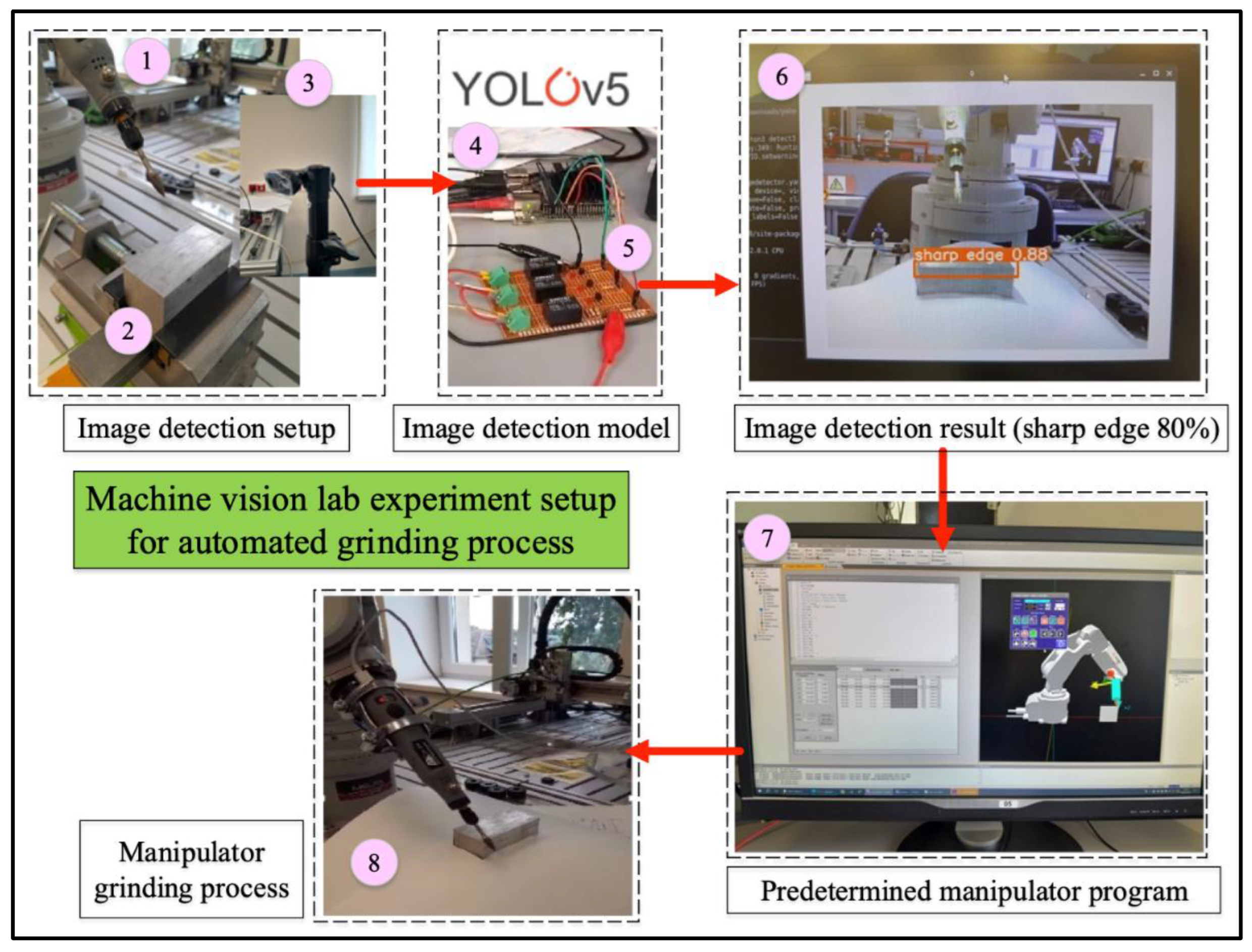
The described experimental setup is based on the complex integration of the Mitsubishi Melfa RV-2F-1D1-S15 manipulator and the YOLOv5 program that is running on a NVIDIA Jetson Nano. The overarching objective is to enable automated chamfering of the metal workpiece based on the detection of sharp edges, chamfer edges, or burrs on their surface. The process commences with the Jetson Nano, with the YOLOv5 program inside. The program is designed to undertake real-time object detection utilizing the input from the connected camera. This camera serves as the sensory input, capturing images of the metal workpiece’s surface. Upon image acquisition, the YOLOv5 program processes the visuals to classify and detect three different images i.e., sharp edge, chamfer edge, and burrs edge of the metal workpiece.
Upon successful detection, the YOLOv5 program initiates the subsequent action. In this instance, it generates a set of distinct class classification commands (sharp edge, chamfer edge, burr edge) in a signal format. Mitsubishi Melfa RV-2F-1D1-S15 robot manipulator receives the polynomial command signal set as the input medium. The manipulator is prepared to receive signals from the machine vision as commands. A detail explanation of the communication from NVIDIA Jetson Nano and Mitsubishi Melfa RV-2F-1D1-S15 robot manipulator is presented in Figure 12’s description No. 5. Depending on the type of signal received, which indicates the presence of an edge image detection, the robot manipulator interprets the signal and initiates the appropriate corrective action. The robot manipulator action is based on the predetermined CAD software which was explain in the first paragraph of this section. The robot have three different actions to accommodate three possible edge detection output from real-time machine vision method. For example, if the sharp image was detected, the robot manipulator was programmed to have 5 passes of grinding and chamfering process. A detail of the three actions based on the machine vision output is presented in Table 6. A simulation of the successful real time machine vision lab experiment is presented in the following YouTube link: https://www.youtube.com/watch?v=Qe6DPEanpjg&t=3s.
Table 6.
Action of robot manipulator based on NVIDIA Jetson Nano prediction output.
| Edge Image Detection (input from Jetson Nano) |
Number of Passes for Grinding and Chamfering (robot manipulator action according to the Jetson Nano input) |
|---|---|
| Sharp | 5 |
| Chamfer | 3 |
| Burrs | 10 |
Description of Figure 12:
- The Mitsubishi Electric Melfa RV-2F-1D1-S15 manipulator was connected to the customized grinding equipment. The end effector was connected to the portable grinder.
- A selected metal workpiece with a sharp type was attached to the clamp close to the manipulator for testing of real-time machine vision method.
- A Logitech camera with 720p and 30 fps was set up to capture the tested metal workpiece with a sharp-end feature.
-
NVIDIA Jetson Nano with embedded YOLOv5 model was connected to a PC and camera. The following is a detail of the embedded system:To begin engagement with it. It is necessary to get the most recent operating system (OS) image known as Jetpack SDK. This software package encompasses the Linux Driver Package (L4T), which consists of the Linux operating system, as well as CUDA-X accelerated libraries and APIs. These components are specifically designed to facilitate Deep Learning, Computer Vision, Accelerated Computing, and Multimedia tasks. The website [45] provides comprehensive documentation, including all necessary materials and step-by-step instructions for utilizing the product. In this project, Ubuntu 20.04 has been utilized, encompassing the most recent iterations of CUDA, cuDNN, and TensorRT, which will be discussed in subsequent sections [46].
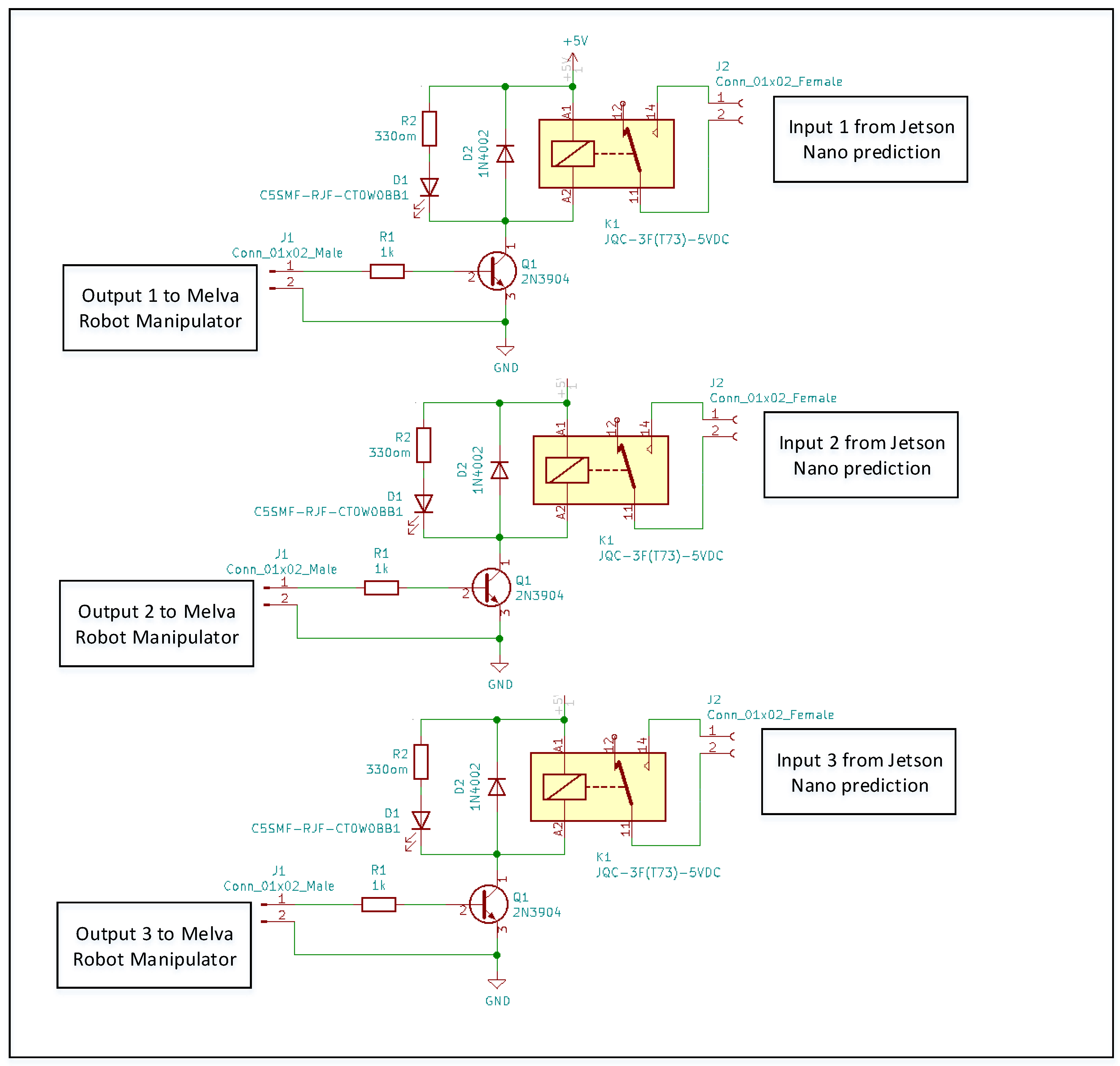
- A customized electrical board was designed as communication hardware between Jetson Nano and the robot manipulator. The communication was done through GPIO (General Purpose Input/Output) pins on the Jetson Nano device. This circuit board translates the output from GPIO inputs to the PLC controller of the manipulator. A detail of electrical circuit board in presented in Figure 13. The board has three inputs and three outputs. The inputs were from the Jetson Nano machine vision image detection result represented in GPIO input and the outputs for the Mitsubishi Electric Melfa RV-2F-1D1-S15 robot manipulator actuator. For example, if the NVIDIA Jetson Nano detect a sharp email, it will goes to GPIO input 1 and go through to output 1 in Mitsubishi Electric Melfa RV-2F-1D1-S15 robot manipulator.
- An image detection of the metal workpiece is shown. It was successfully detected as a sharp edge with a probability of 88%.
- The manipulator has been programmed initially as an action of the image detection from the Jetson Nano.
- The manipulator does the grinding process according to the result of the Jetson Nano that has been interpreted by the customized electrical circuit and the predetermined manipulator program.
Figure 13.
A customized electronic circuit board.
7. Conclusions
The tree DL methods (VGG-16, ResNet, and YOLOv5) with has potential application for machine vision technologies has been studied and examined. These vision algorithms were used to classify and detect three different edge conditions of metal workpieces i.e., sharp edge, chamfer edge, and burrs edge with a satisfactory result. Integration of embedded selected DL method i.e., YOLOv5 model in NVIDIA Jetson Nano microprocessor with Mitsubishi Electric Melfa RV-2F-1D1-S15 manipulator has also been presented. The embedded system and the integrated system were demonstrated in the lab experiment as a potential machine vision approach for automated manufacturing process. For real application in practice or industry, the machine vision system-based YOLOv5 algorithm is integrated with the robot manipulator as the actuator of the predicted outcome as demonstrated in this study.
The integration shows that the YOLOv5 model in real-time image detection provides efficient results in identifying the suggested conditions and classifying them correctly. The stability of this system also improved the efficiency and reliability of the automated system making them suitable for industrial applications, especially in manufacturing applications.
This study contribute in the development of the real-time machine vision system based on YOLOv5 and NVIDIA Jetson Nano in the lab experimental study. The machine vision system was successfully integrated with a Mitsubishi Electric Melfa RV-2F-1D1-S15 robot manipulator to perform automate grinding and chamfering.
The future work of the study:
- The present study used YOLOv5 for the embedded machine vision algorithm, and will try YOLOv8 in the further study.
- Three different edge condition were used in present study. As there are a number of edge condition in practice such as crack and chip, future study will use more than 3 different edge condition.
- A similar size of the metal workpiece is maintain in the present study. In the future different size (length, height, and weight) will be considered for the real-time machine vision system.
- The Mitsubishi Electric Melfa RV-2F-1D1-S15 robot manipulator, which is equipped with a chamfering tool attached to the tooltip, serves as the medium for automatic intervention. The present study has successfully deliver an experimental study. In the future, in the event of the presence of sharp edges or burrs, the manipulator employs a chamfering tool to modify the surface of the metal workpiece. This process is repeated until the edge of the metal workpiece becomes appropriately blunted, thereby effectively correcting the defect.
Author Contributions
Conceptualization W.C.; methodology, A.W.K. and W.C.; software, A.W.K. and P.M.; validation, A.W.K. and W.C.; formal analysis, A.W.K., P.M. and W.C.; investigation, W.C.; resources, P.M., G.B., M.B. and W.C.; data curation, A.W.K., P.M., G.B. and M.B.; writing—original draft preparation, A.W.K., P.M. and W.C.; writing—review and editing, A.W.K., P.M., N.A.A. and W.C.; visualization, A.W.K., P.M. and W.C.; supervision, H.Y., G.K. and W.C.; project administration, G.K. and W.C.; funding acquisition, G.K. and W.C.
Funding
The authors acknowledge the Polish National Agency for Academic Exchange (NAWA) No. BPN/ULM/2022/1/00139 for financial support.
Data Availability Statement
Data is available upon request to the corresponding author.
Acknowledgments
The authors appreciate the support from the Department of Control Science and Engineering, Opole University of Technology for facilitating Lab experiments for software-to-hardware utilizing Mitsubishi Electric Melfa RV-2F-1D1-S15.
Conflicts of Interest
The authors declare no conflicts of interest.
References
- Park, M.; Jeong, J. Design and Implementation of Machine Vision-Based Quality Inspection System in Mask Manufacturing Process. Sustainability 2022, 14, 6009. [Google Scholar] [CrossRef]
- Psarommatis, F.; May, G.; Dreyfus, P.-A.; Kiritsis, D. Zero Defect Manufacturing: State-of-the-Art Review, Shortcomings and Future Directions in Research. International Journal of Production Research 2020, 58, 1–17. [Google Scholar] [CrossRef]
- Powell, D.; Magnanini, M.C.; Colledani, M.; Myklebust, O. Advancing Zero Defect Manufacturing: A State-of-the-Art Perspective and Future Research Directions. Computers in Industry 2022, 136, 103596. [Google Scholar] [CrossRef]
- Zhou, J.; Li, P.; Zhou, Y.; Wang, B.; Zang, J.; Meng, L. Toward New-Generation Intelligent Manufacturing. Engineering 2018, 4, 11–20. [Google Scholar] [CrossRef]
- Yang, X.; Han, M.; Tang, H.; Li, Q.; Luo, X. Detecting Defects With Support Vector Machine in Logistics Packaging Boxes for Edge Computing. IEEE Access 2020, 8, 64002–64010. [Google Scholar] [CrossRef]
- C. Hui; B. Xingcan; L. Mingqi Research on Image Edge Detection Method Based on Multi-Sensor Data Fusion. In Proceedings of the 2020 IEEE International Conference on Artificial Intelligence and Computer Applications (ICAICA); June 27 2020; pp. 789–792.
- Yang, X.; Han, M.; Tang, H.; Li, Q.; Luo, X. Detecting Defects With Support Vector Machine in Logistics Packaging Boxes for Edge Computing. IEEE Access 2020, 8, 64002–64010. [Google Scholar] [CrossRef]
- Wittmann, J.; Herl, G.; Deggendorf Institute of Technology. Canny-Net: Known Operator Learning for Edge Detection. eJNDT 2023, 28. [Google Scholar] [CrossRef]
- S. Lei; Y. Guo; Y. Liu; F. Li; G. Zhang; D. Yang Detection of Mechanical Defects of High Voltage Circuit Breaker Based on Improved Edge Detection and Deep Learning Algorithms. In Proceedings of the 2022 6th International Conference on Electric Power Equipment - Switching Technology (ICEPE-ST), 15 March 2022; pp. 372–375.
- Zhou, L.; Zhang, L.; Konz, N. Computer Vision Techniques in Manufacturing 2022.
- González, M.; Rodríguez, A.; López-Saratxaga, U.; Pereira, O.; López De Lacalle, L.N. Adaptive Edge Finishing Process on Distorted Features through Robot-Assisted Computer Vision. Journal of Manufacturing Systems 2024, 74, 41–54. [Google Scholar] [CrossRef]
- Han, D.; Mulyana, B.; Stankovic, V.; Cheng, S. A Survey on Deep Reinforcement Learning Algorithms for Robotic Manipulation. Sensors 2023, 23, 3762. [Google Scholar] [CrossRef]
- Ichnowski, J.; Avigal, Y.; Satish, V.; Goldberg, K. Deep Learning Can Accelerate Grasp-Optimized Motion Planning. Sci. Robot. 2020, 5, eabd7710. [Google Scholar] [CrossRef]
- Qiu, S.; Yang, Z.; Huang, L.; Zhang, X. Design and Implementation of Temperature Verification System Based on Robotic Arm. J. Phys.: Conf. Ser. 2022, 2203, 012015. [Google Scholar] [CrossRef]
- Ban, S.; Lee, Y.J.; Yu, K.J.; Chang, J.W.; Kim, J.-H.; Yeo, W.-H. Persistent Human–Machine Interfaces for Robotic Arm Control Via Gaze and Eye Direction Tracking. Advanced Intelligent Systems 2023, 5, 2200408. [Google Scholar] [CrossRef]
- Sekkat, H.; Tigani, S.; Saadane, R.; Chehri, A. Vision-Based Robotic Arm Control Algorithm Using Deep Reinforcement Learning for Autonomous Objects Grasping. Applied Sciences 2021, 11, 7917. [Google Scholar] [CrossRef]
- Kijdech, D.; Vongbunyong, S. Pick-and-Place Application Using a Dual Arm Collaborative Robot and an RGB-D Camera with YOLOv5. IJRA 2023, 12, 197. [Google Scholar] [CrossRef]
- Aein, S.; Thu, T.; Htun, P.; Paing, A.; Htet, H. YOLO Based Deep Learning Network for Metal Surface Inspection System. In; 2022; pp. 923–929 ISBN 978-981-16-8128-8.
- Li, J.; Su, Z.; Geng, J.; Yin, Y. Real-Time Detection of Steel Strip Surface Defects Based on Improved YOLO Detection Network. IFAC-PapersOnLine 2018, 51, 76–81. [Google Scholar] [CrossRef]
- Xu, Y.; Zhang, K.; Wang, L. Metal Surface Defect Detection Using Modified YOLO. Algorithms 2021, 14, 257. [Google Scholar] [CrossRef]
- Ahmed, S.; Bhatti, M.T.; Khan, M.G.; Lövström, B.; Shahid, M. Development and Optimization of Deep Learning Models for Weapon Detection in Surveillance Videos. Applied Sciences 2022, 12, 5772. [Google Scholar] [CrossRef]
- Fahd Al-Selwi, H.; Hassan, N.; Ab Ghani, H.B.; Binti Amir Hamzah, N.A.; Bin, A.; Aziz, A. Face Mask Detection and Counting Using You Only Look Once Algorithm with Jetson Nano and NVDIA Giga Texel Shader Extreme. IJ-AI 2023, 12, 1169. [Google Scholar] [CrossRef]
- Abdul Hassan, N.F.; Abed, A.A.; Abdalla, T.Y. Face Mask Detection Using Deep Learning on NVIDIA Jetson Nano. IJECE 2022, 12, 5427. [Google Scholar] [CrossRef]
- D. -L. Nguyen; M. D. Putro; K. -H. Jo Facemask Wearing Alert System Based on Simple Architecture With Low-Computing Devices. IEEE Access 2022, 10, 29972–29981. [Google Scholar] [CrossRef]
- H. Feng; G. Mu; S. Zhong; P. Zhang; T. Yuan Benchmark Analysis of YOLO Performance on Edge Intelligence Devices. In Proceedings of the 2021 Cross Strait Radio Science and Wireless Technology Conference (CSRSWTC); October 11 2021; pp. 319–321.
- Saponara, S.; Elhanashi, A.; Gagliardi, A. Implementing a Real-Time, AI-Based, People Detection and Social Distancing Measuring System for Covid-19. J Real Time Image Process 2021, 18, 1937–1947. [Google Scholar] [CrossRef] [PubMed]
- H. -S. Son; D. -K. Kim; S. -H. Yang; Y. -K. Choi Real-Time Power Line Detection for Safe Flight of Agricultural Spraying Drones Using Embedded Systems and Deep Learning. IEEE Access 2022, 10, 54947–54956. [Google Scholar] [CrossRef]
- Qasim, M.; Ismael, O.Y. Shared Control of a Robot Arm Using BCI and Computer Vision. JESA 2022, 55, 139–146. [Google Scholar] [CrossRef]
- MIZUMOTO, Y.; ASAKAWA, N.; Morishige, K.; TAKEUCHI, Y. Automation of Chamfering with Industrial Robot : Application of Improved Intelligent Holder. The proceedings of the JSME annual meeting 2000, 3, 537–538. [Google Scholar] [CrossRef]
- Giuffrida, G.; Meoni, G.; Fanucci, L. A YOLOv2 Convolutional Neural Network-Based Human–Machine Interface for the Control of Assistive Robotic Manipulators. Applied Sciences 2019, 9, 2243. [Google Scholar] [CrossRef]
- Nantzios, G.; Baras, N.; Dasygenis, M. Design and Implementation of a Robotic Arm Assistant with Voice Interaction Using Machine Vision. Automation 2021, 2, 238–251. [Google Scholar] [CrossRef]
- Pranoto, K.A.; Caesarendra, W.; Petra, I. Burrs and Sharp Edge Detection of Metal Workpiece Using CNN Image Classification Method for Intelligent Manufacturing Application.
- Ibrahim, A.A.M.S.; Tapamo, J.R. Transfer Learning-Based Approach Using New Convolutional Neural Network Classifier for Steel Surface Defects Classification. Scientific African 2024, 23, e02066. [Google Scholar] [CrossRef]
- Jarkas, O.; Hall, J.; Smith, S.; Mahmud, R.; Khojasteh, P.; Scarsbrook, J.; Ko, R.K.L. ResNet and Yolov5-Enabled Non-Invasive Meat Identification for High-Accuracy Box Label Verification. Engineering Applications of Artificial Intelligence 2023, 125, 106679. [Google Scholar] [CrossRef]
- Chen, C.; Gu, H.; Lian, S.; Zhao, Y.; Xiao, B. Investigation of Edge Computing in Computer Vision-Based Construction Resource Detection. Buildings 2022, 12, 2167. [Google Scholar] [CrossRef]
- Roy, A.M.; Bhaduri, J. DenseSPH-YOLOv5: An Automated Damage Detection Model Based on DenseNet and Swin-Transformer Prediction Head-Enabled YOLOv5 with Attention Mechanism. Advanced Engineering Informatics 2023, 56, 102007. [Google Scholar] [CrossRef]
- Zhang, Y.-F.; Ren, W.; Zhang, Z.; Jia, Z.; Wang, L.; Tan, T. Focal and Efficient IOU Loss for Accurate Bounding Box Regression 2022.
- Yap, M.H.; Hachiuma, R.; Alavi, A.; Brüngel, R.; Cassidy, B.; Goyal, M.; Zhu, H.; Rückert, J.; Olshansky, M.; Huang, X.; et al. Deep Learning in Diabetic Foot Ulcers Detection: A Comprehensive Evaluation. Computers in Biology and Medicine 2021, 135, 104596. [Google Scholar] [CrossRef] [PubMed]
- He, K.; Zhang, X.; Ren, S.; Sun, J. Deep Residual Learning for Image Recognition. In Proceedings of the 2016 IEEE Conference on Computer Vision and Pattern Recognition (CVPR), Las Vegas, NV, USA, June 2016; pp. 770–778. [Google Scholar]
- Veit, A.; Wilber, M.; Belongie, S. Residual Networks Behave Like Ensembles of Relatively Shallow Networks.
- Padilla, R.; Passos, W.L.; Dias, T.L.B.; Netto, S.L.; Da Silva, E.A.B. A Comparative Analysis of Object Detection Metrics with a Companion Open-Source Toolkit. Electronics 2021, 10, 279. [Google Scholar] [CrossRef]
- Chicco, D.; Jurman, G. The Advantages of the Matthews Correlation Coefficient (MCC) over F1 Score and Accuracy in Binary Classification Evaluation. BMC Genomics 2020, 21, 6. [Google Scholar] [CrossRef] [PubMed]
- Lindholm, A.; Wahlström, N.; Lindsten, F.; Schön, T.B. Machine Learning: A First Course for Engineers and Scientists, 1st ed.; Cambridge University Press: Cambridge, UK, 2022; ISBN 978-1-108-91937-1. [Google Scholar]
- Cai, W.; Xiong, Z.; Sun, X.; Rosin, P.L.; Jin, L.; Peng, X. Panoptic Segmentation-Based Attention for Image Captioning. Applied Sciences 2020, 10, 391. [Google Scholar] [CrossRef]
- Nvidia Developer JetPack SDK. Available online: https://developer.nvidia.com/embedded/jetpack (accessed on 9 September 2024).
- NVIDIA Corporation NVIDIA Jetson Nano. Available online: https://www.nvidia.com/en-us/autonomous-machines/embedded-systems/jetson-nano/product-development/ (accessed on 9 September 2024).
Figure 1.
VGG-16 architecture.
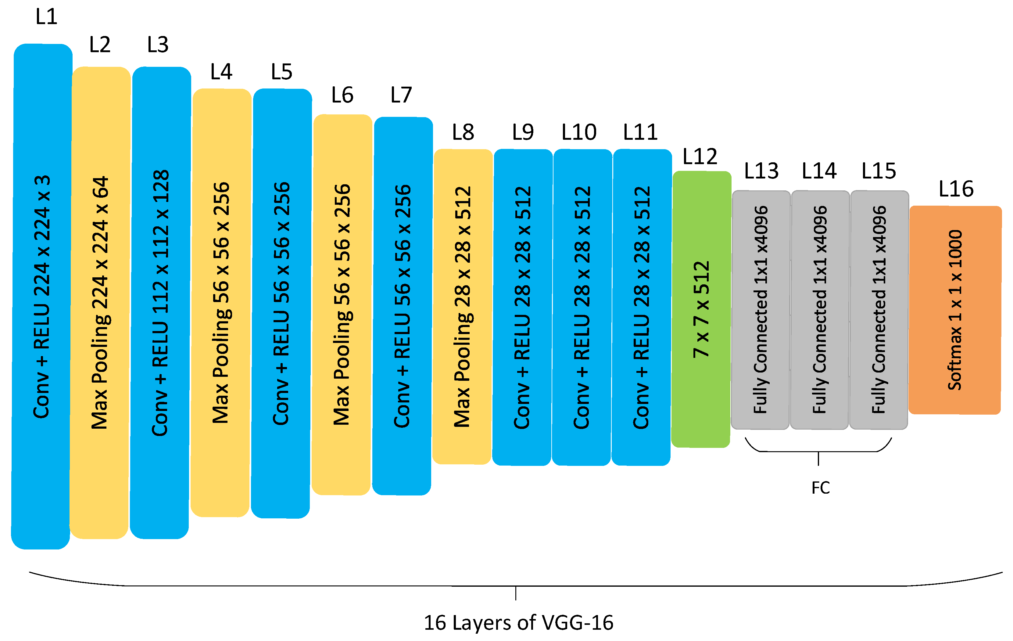
Figure 2.
YOLOv5 architecture.
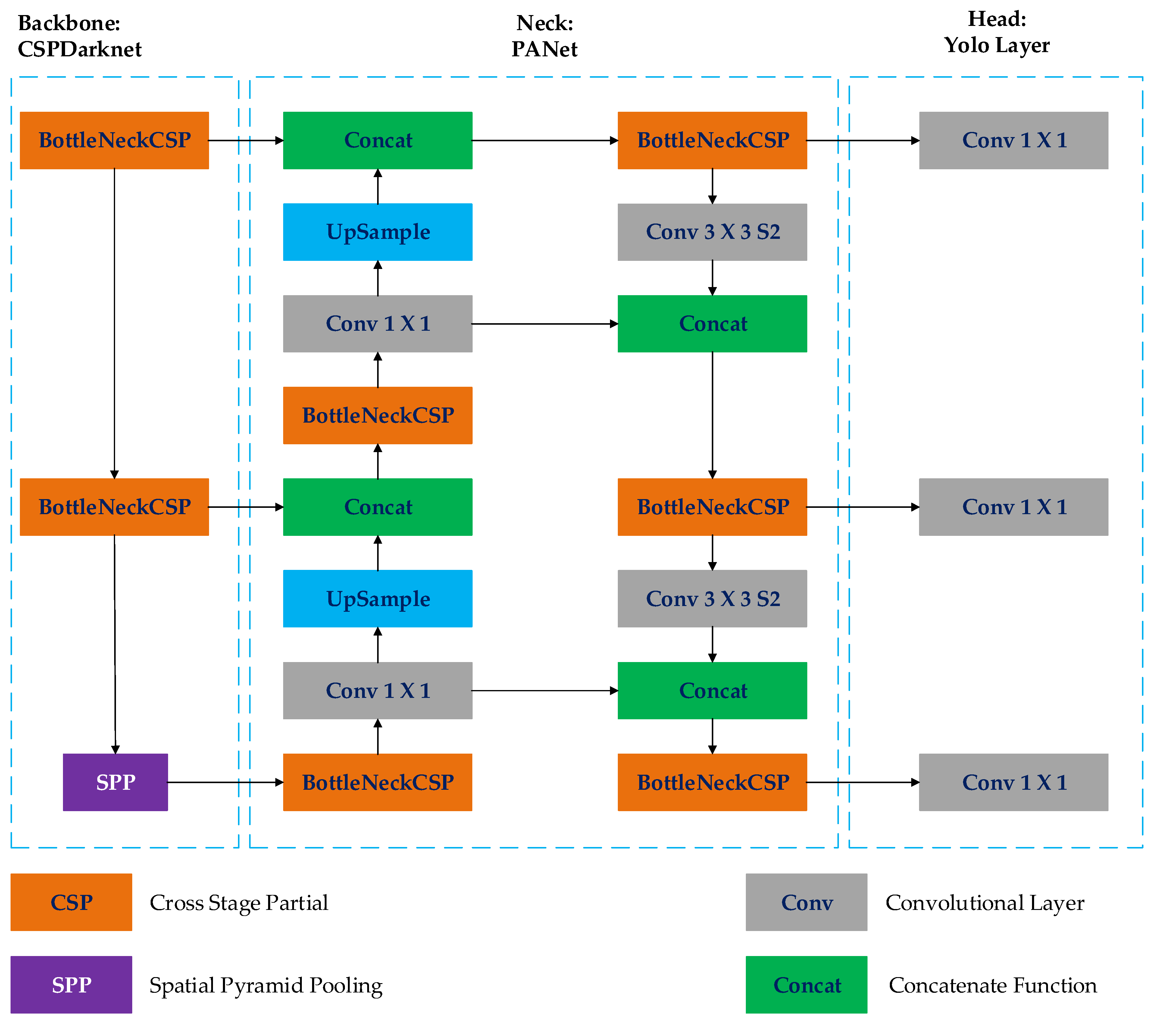
Figure 3.
ResNet architecture.
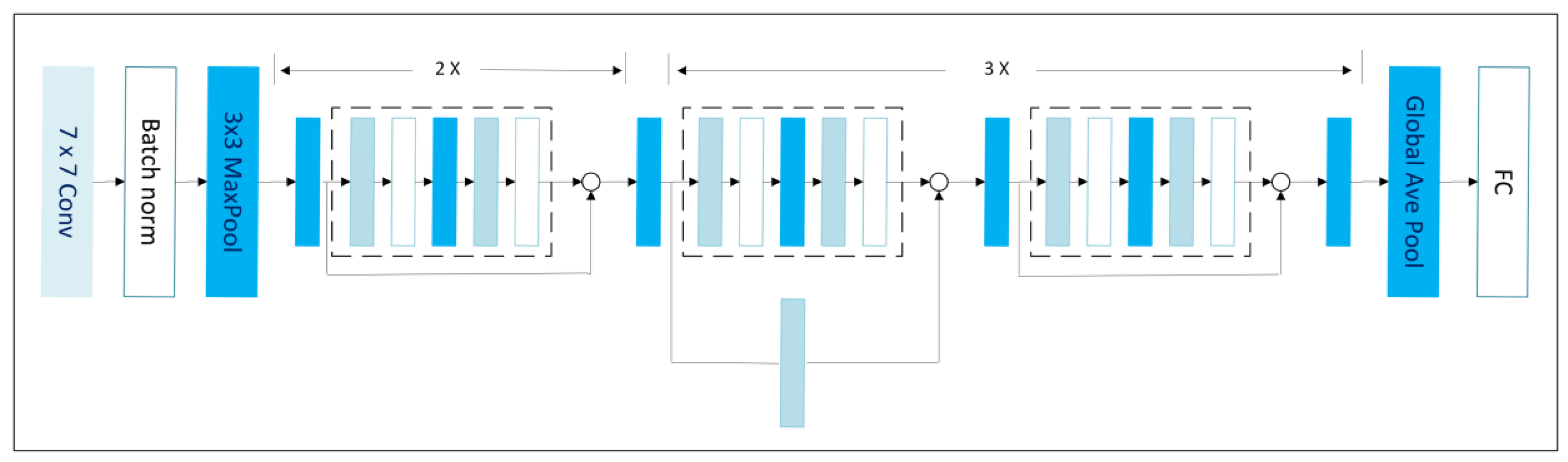
Figure 4.
Illustration of IoU equation. Adapted from [41].
Figure 4.
Illustration of IoU equation. Adapted from [41].
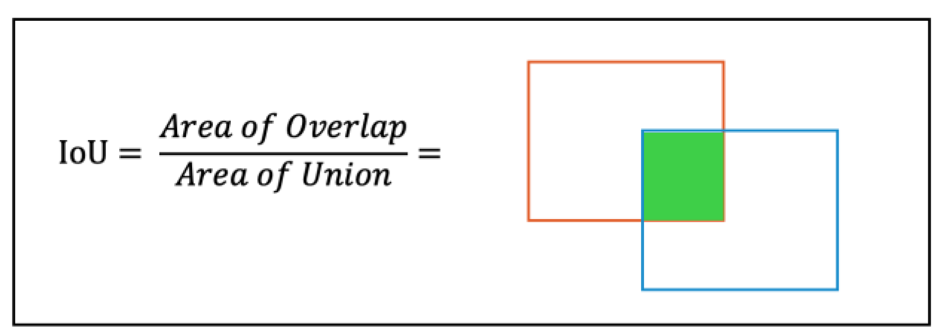
Figure 5.
ROC curve.
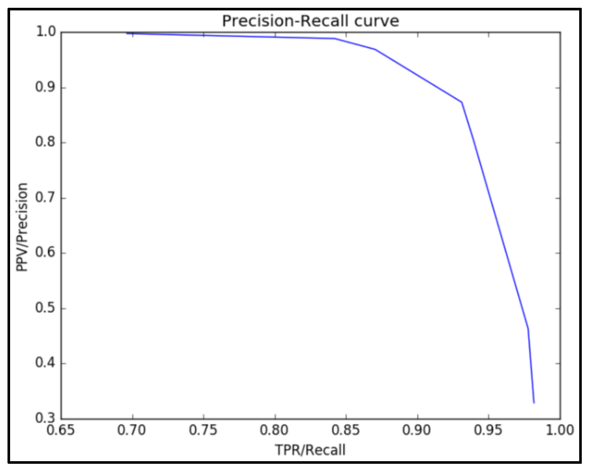
Figure 6.
Flowchart of overall methodology.
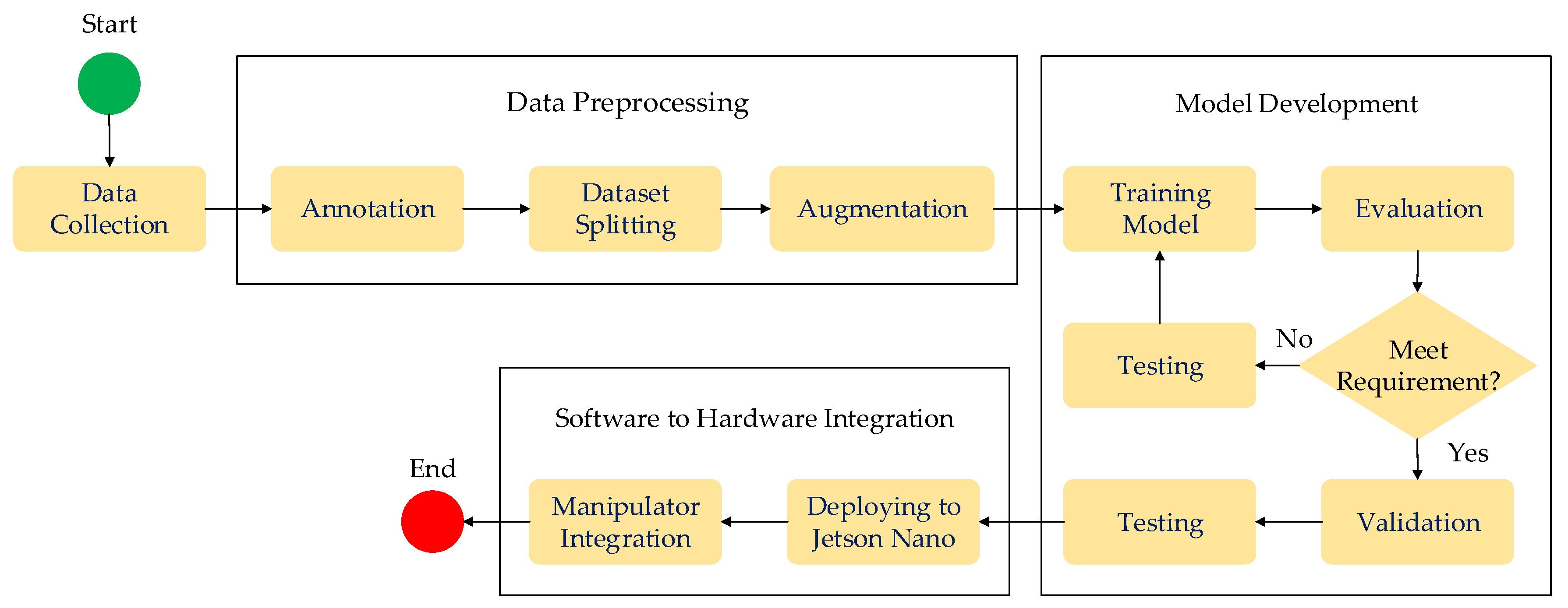
Figure 7.
Augmentation on the dataset.
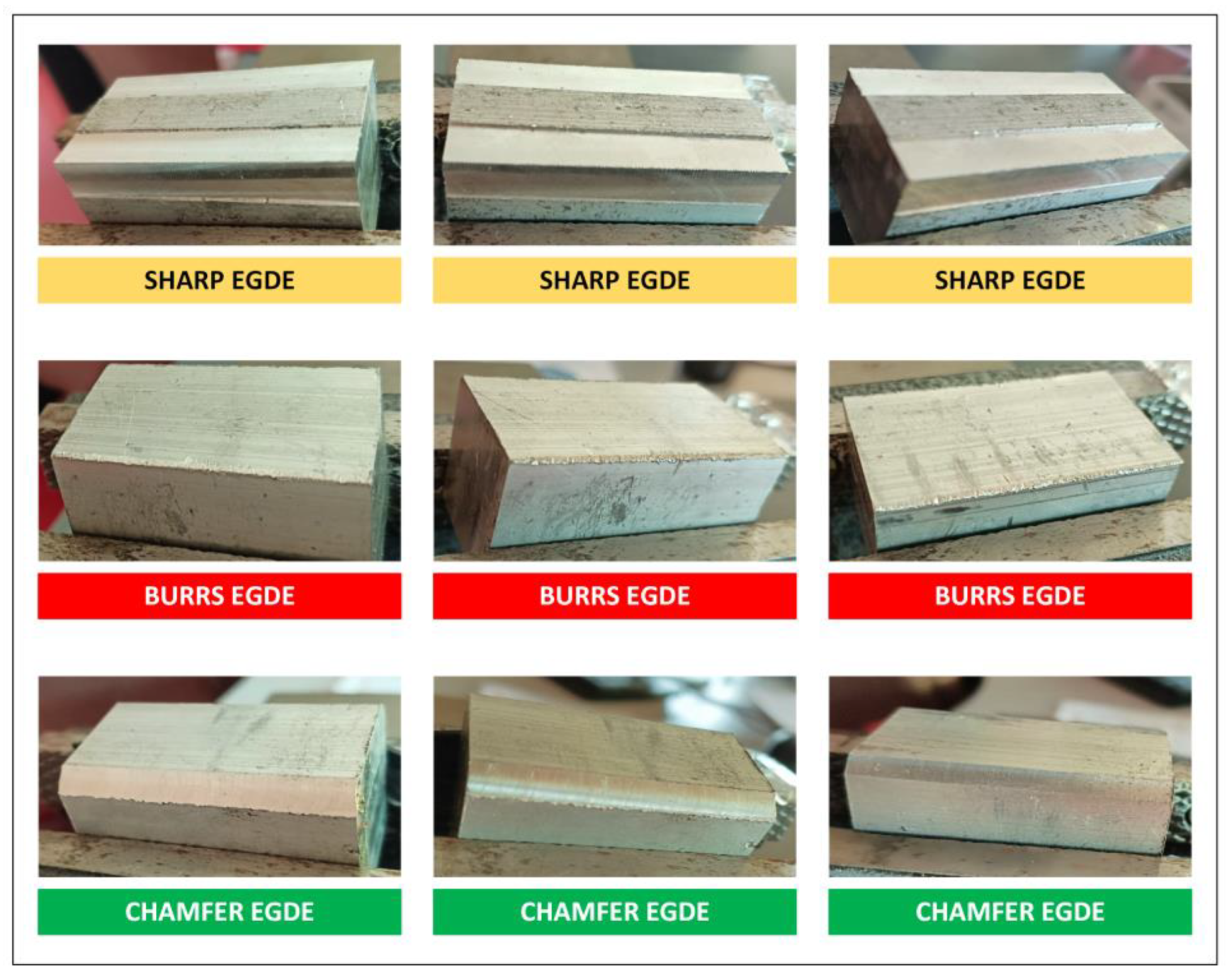
Figure 8.
mAP of VGG-16.
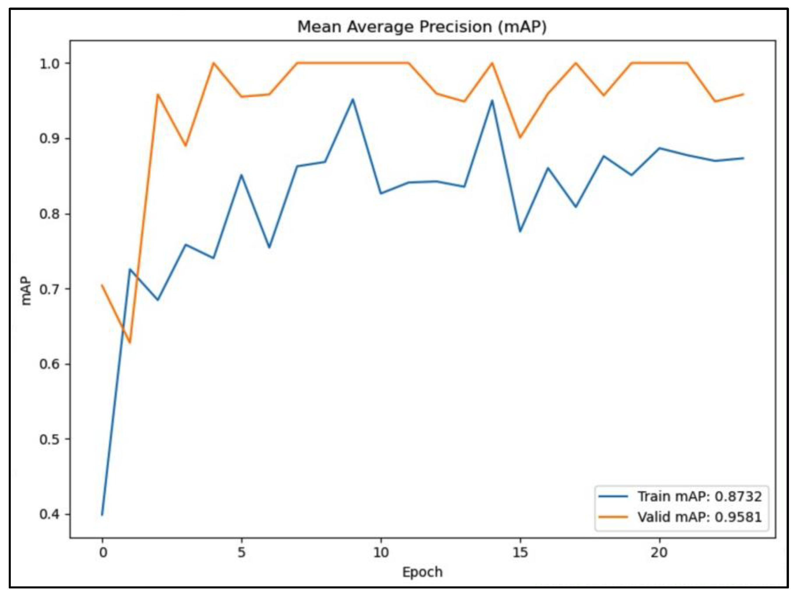
Figure 9.
mAP of ResNet.
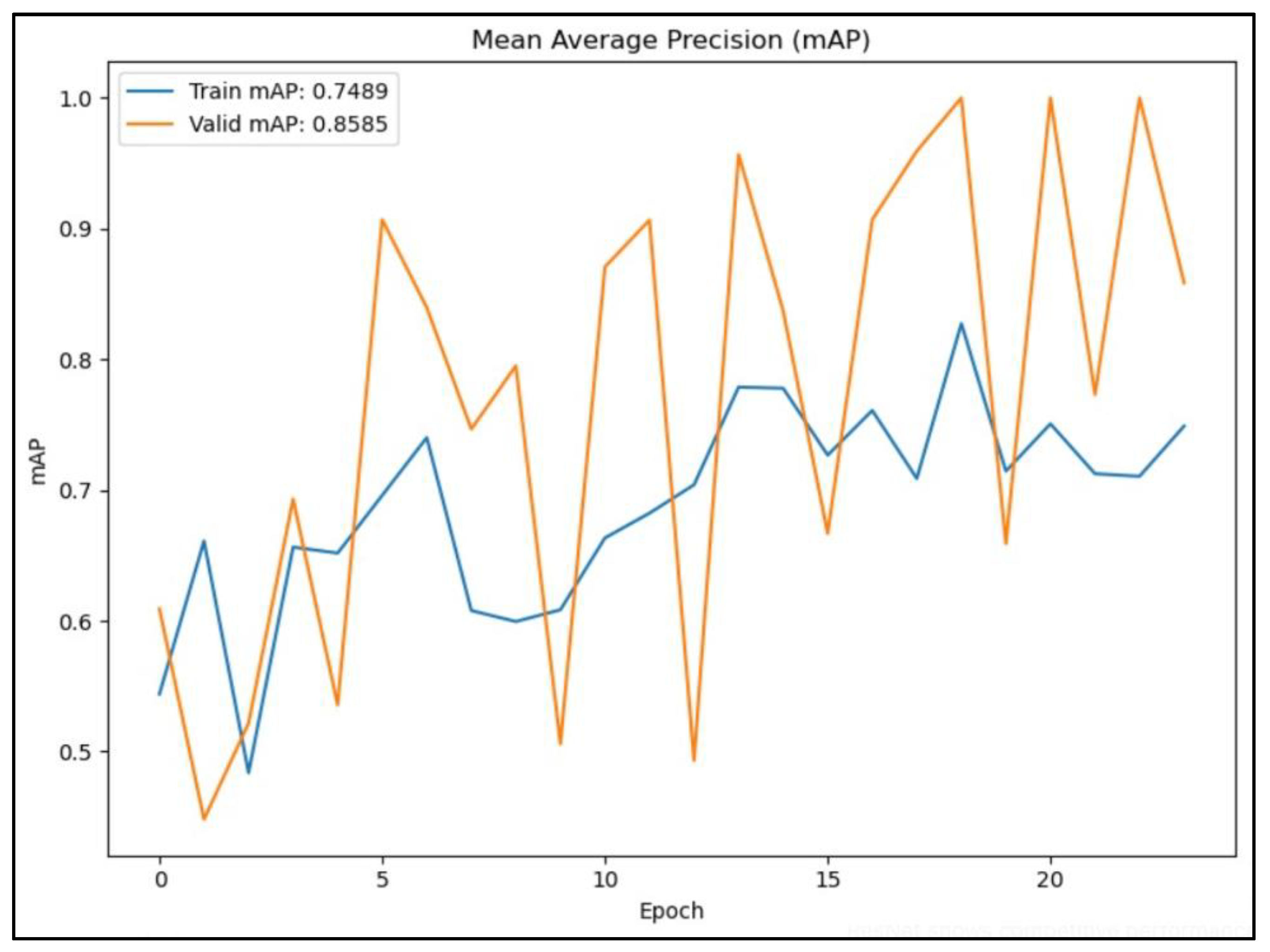
Figure 10.
mAP of YOLOv5.
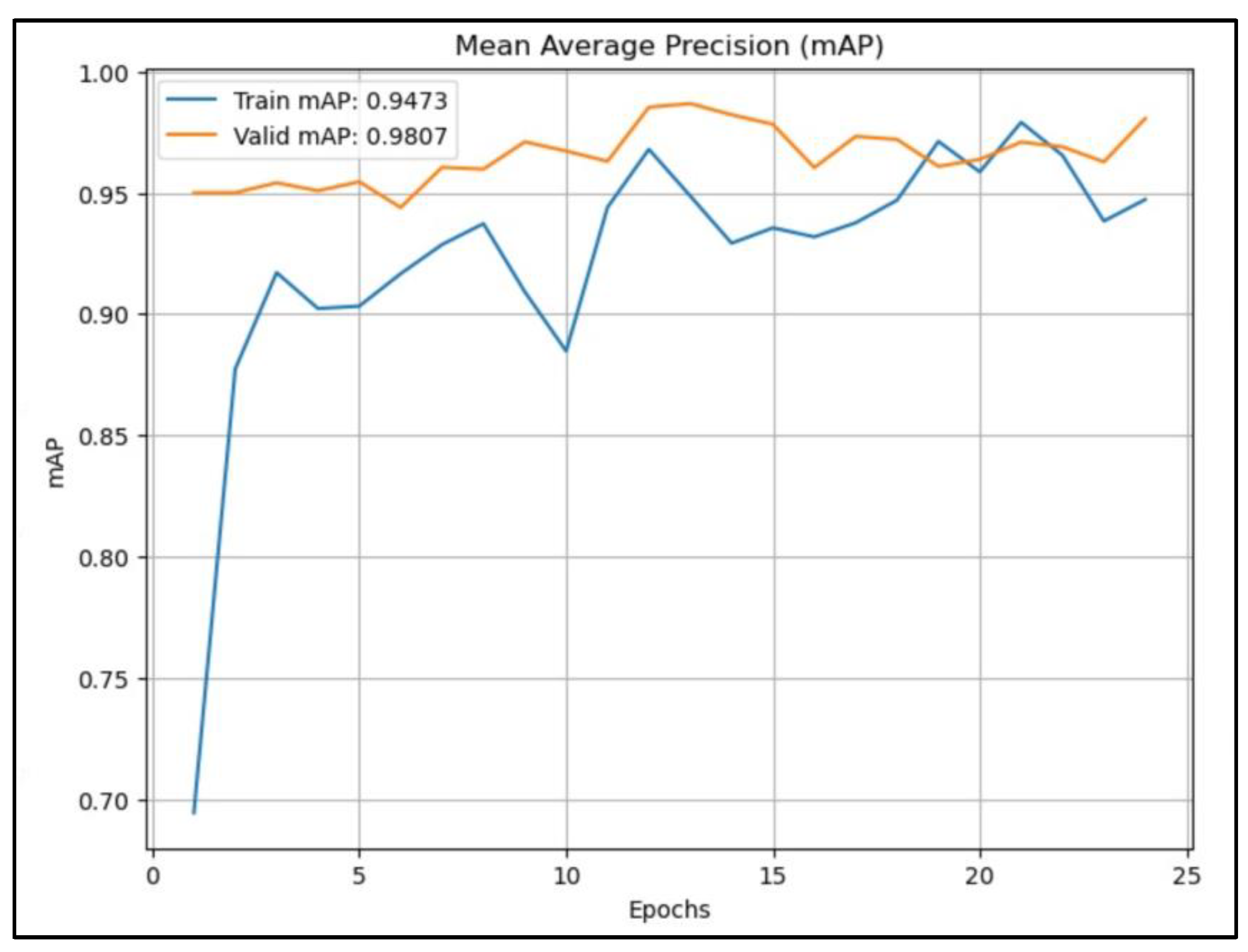
Figure 11.
Loss model of VGG-16.
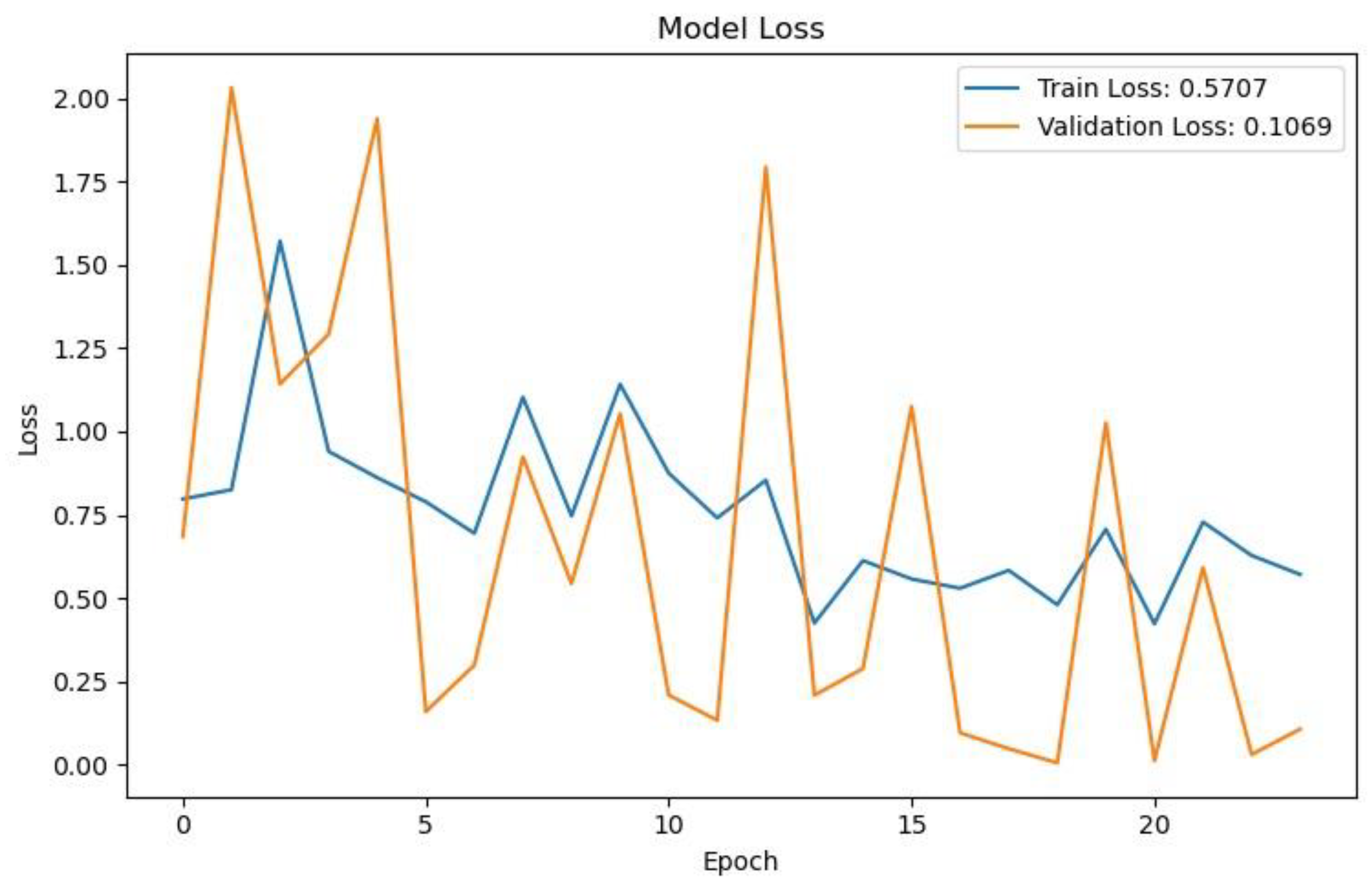
Figure 12.
Loss model of ResNet.
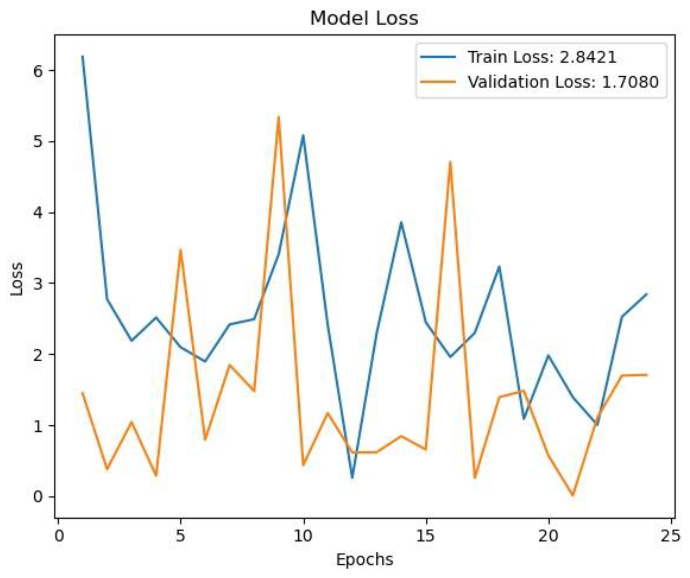
Figure 13.
Loss model of YOLOv5.
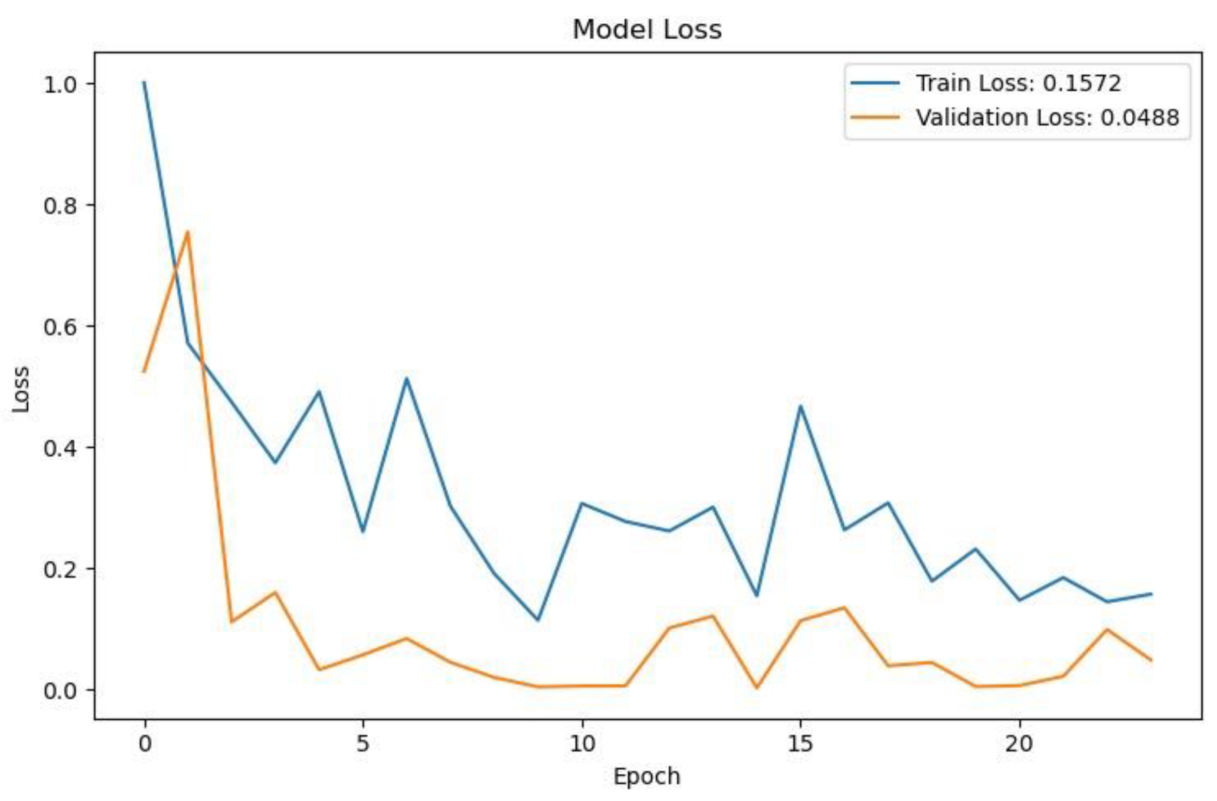
Figure 14.
VGG-16 precision-recall.
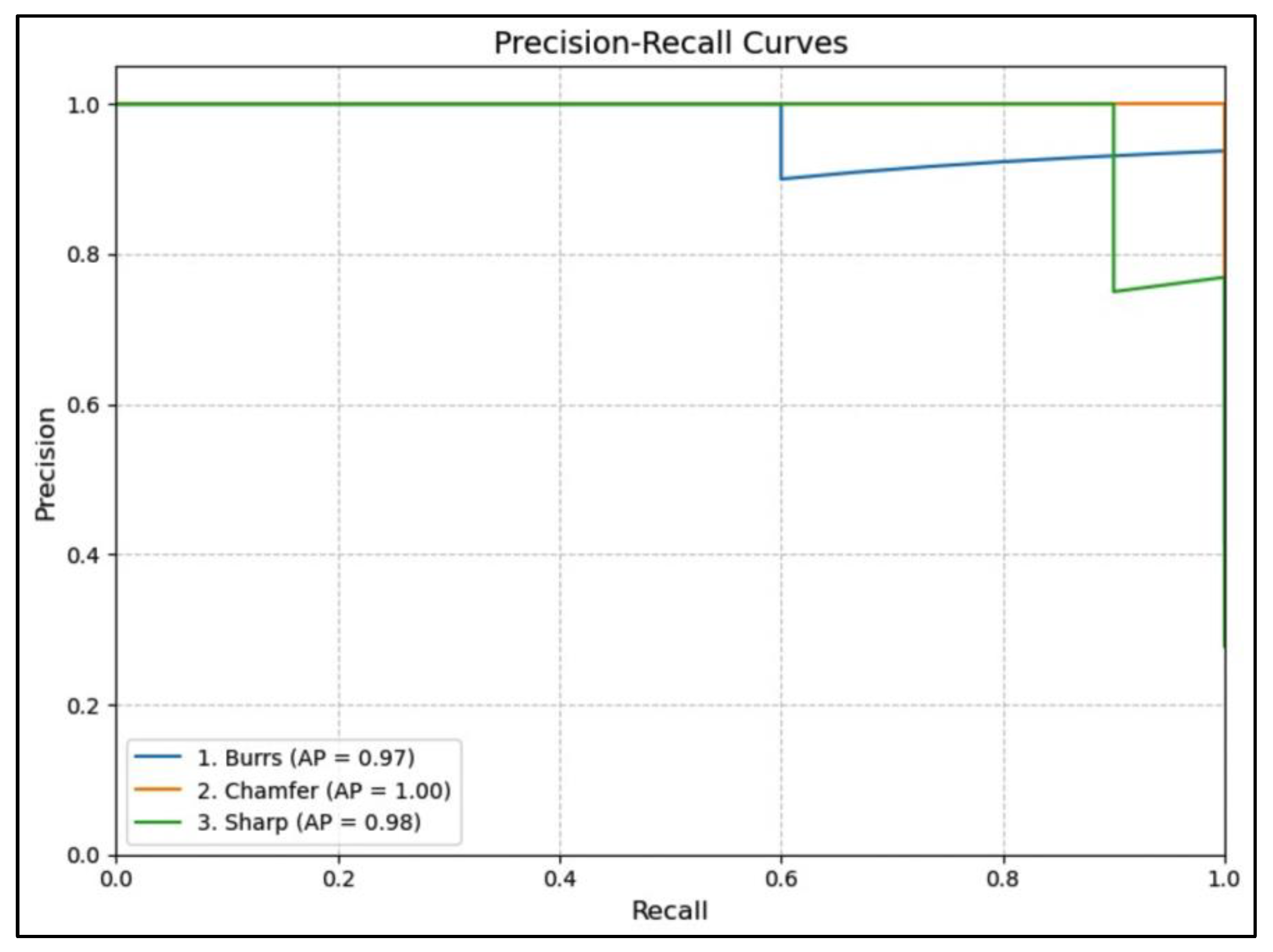
Figure 15.
ResNet precision-recall.
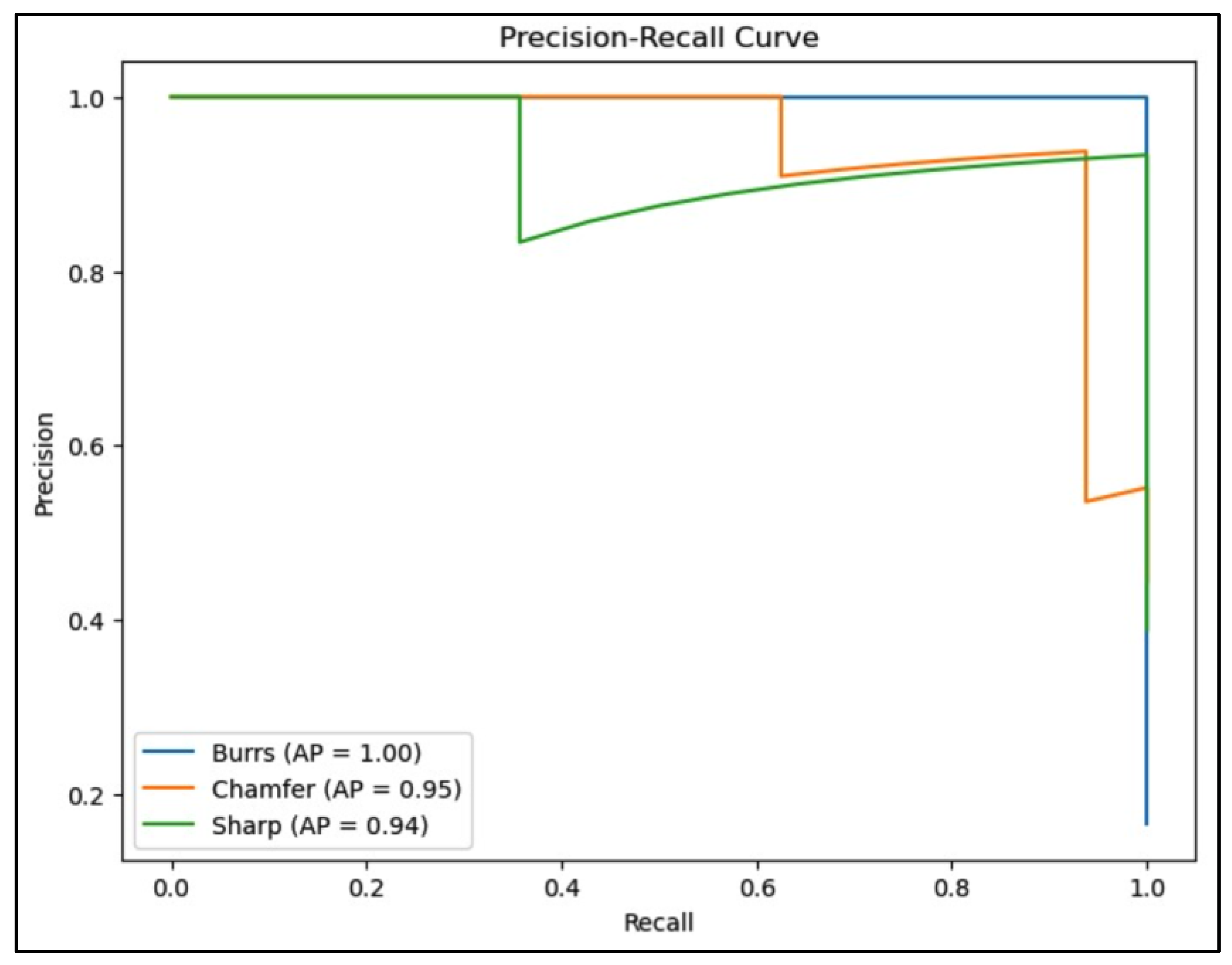
Figure 16.
YOLOv5 precision-recall.
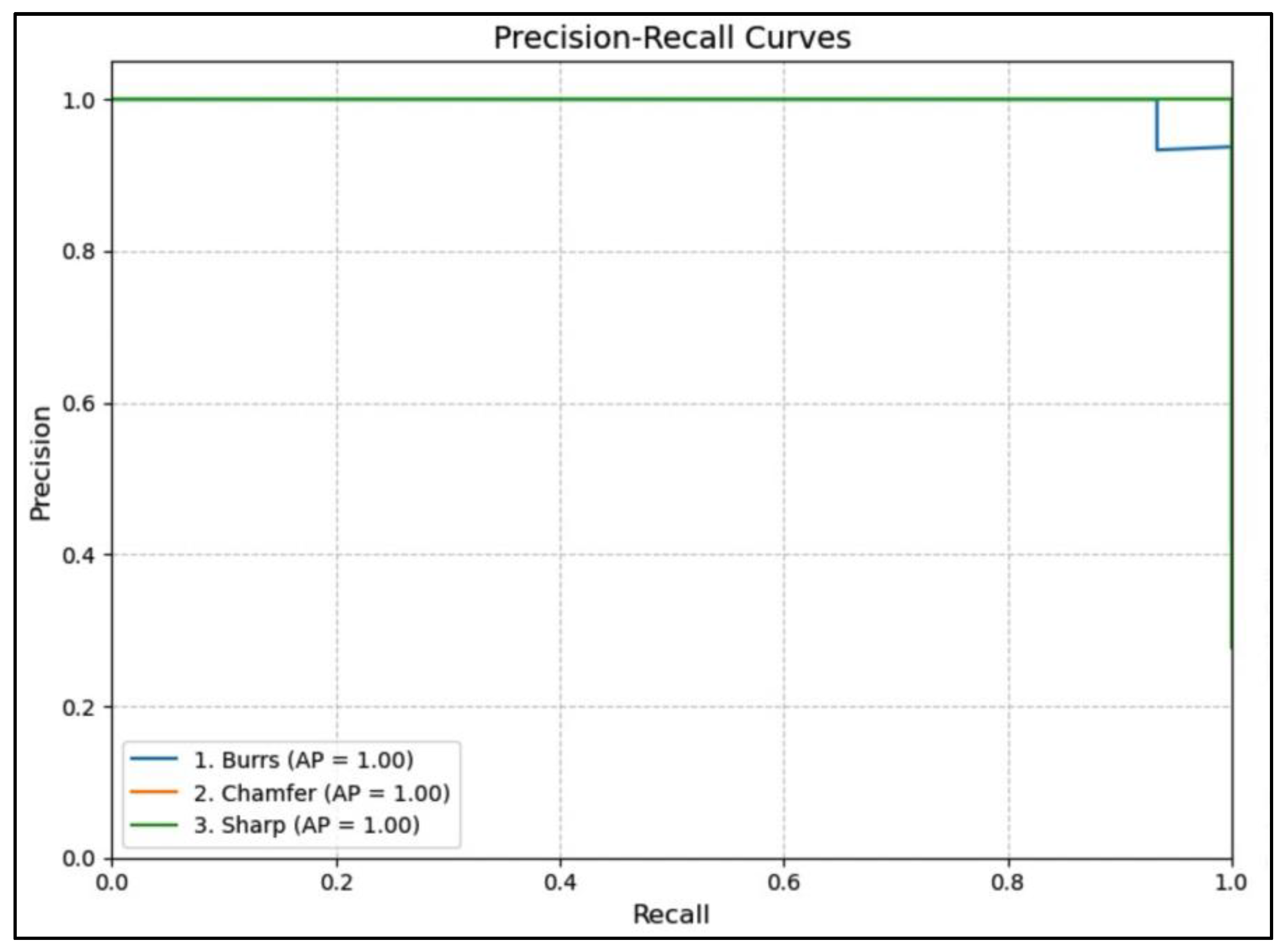
Figure 17.
Confusion matrix of VGG-16.
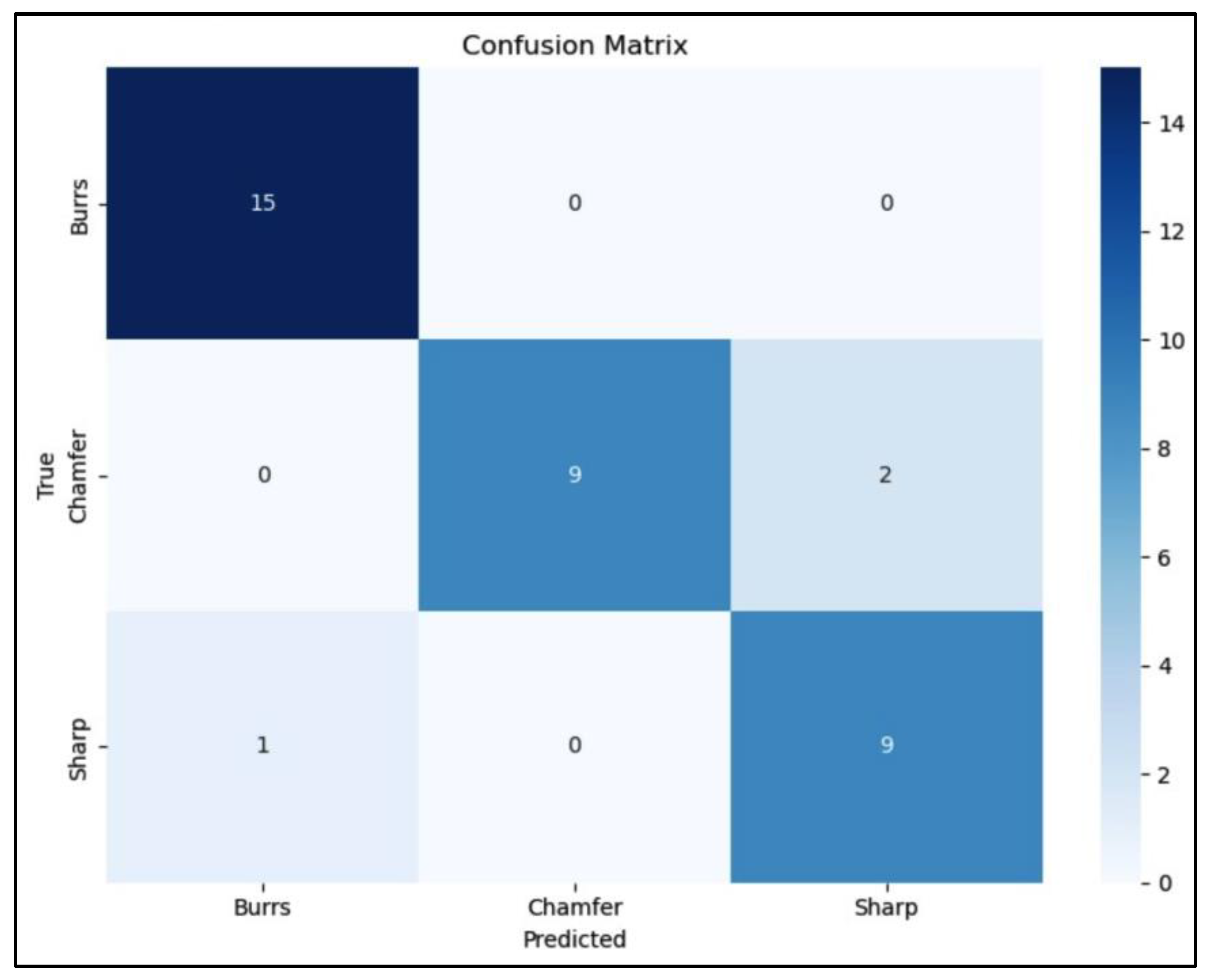
Figure 18.
Confusion matrix of ResNet.
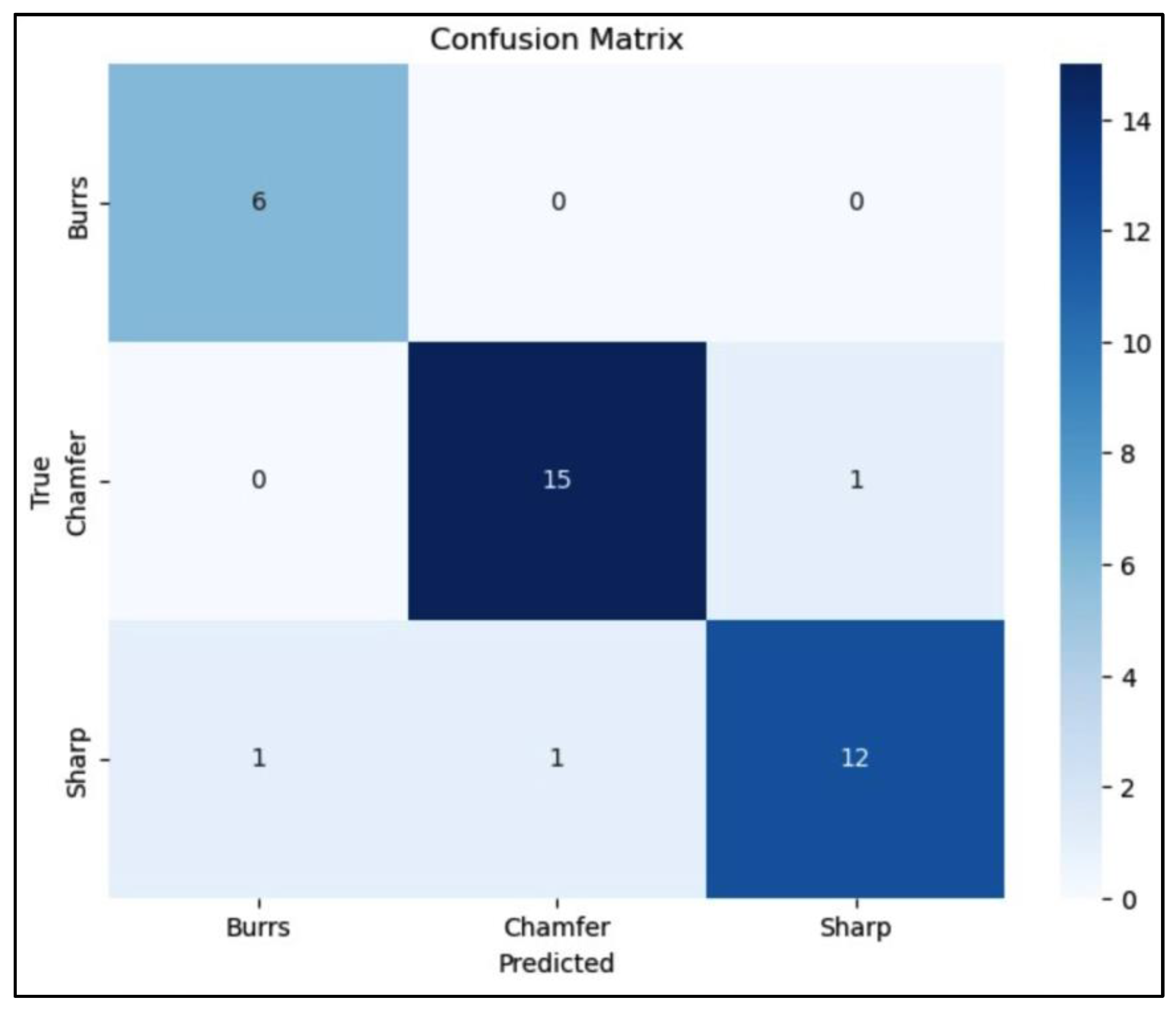
Figure 19.
Confusion matrix of YOLOv5.
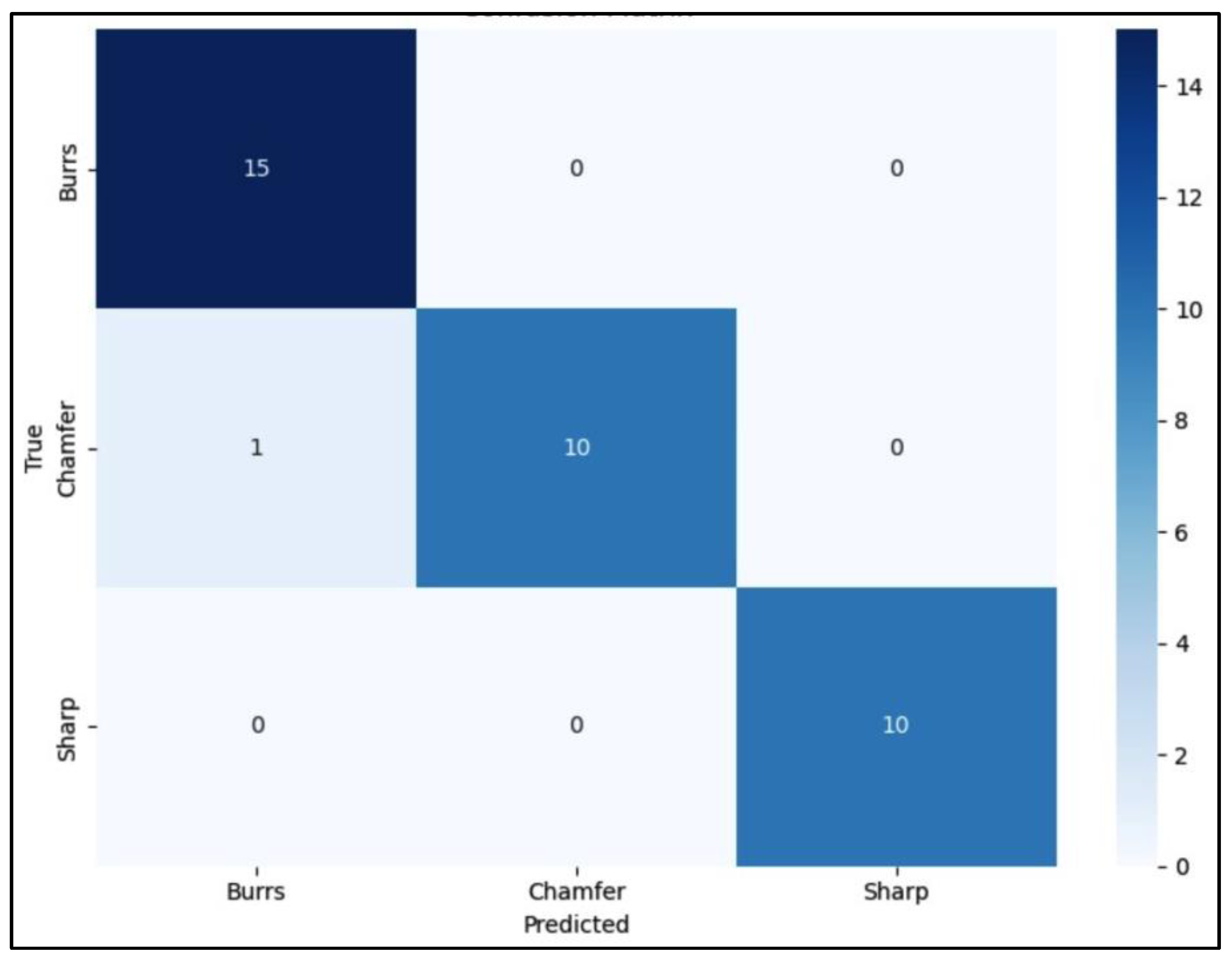
Table 3.
Label distribution.
| Total number of annotations | Sharp edge | Chamfer edge | Burrs edge |
|---|---|---|---|
| 300 | 100 | 100 | 100 |
| 100% | 33.33% | 33.33% | 33.33% |
Table 4.
Distributed images.
| Number of images | Training | Validation | Testing |
|---|---|---|---|
| 300 | 210 | 45 | 45 |
| 100% | 70% | 15% | 15% |
Table 5.
Hyperparameter settings.
| Hyperparameter | Value/Description |
|---|---|
| Batch size | 8 |
| Epochs | 24 |
| Image size | 224 x 224 |
| Learning rate (YOLOv5) | 0.01 |
| Learning rate (VGG16) | 0.001 |
| Learning rate (ResNet) | 0.001 |
| Optimizer | Adam |
Table 6.
Models performance of three DL models.
| Model | Accuracy | mAP | Avg. Precision | Avg. Recall | Avg. F1-Score |
|---|---|---|---|---|---|
| VGG-16 | 0.92 | 0.95 | 0.91 | 0.93 | 0.92 |
| ResNet | 0.92 | 0.85 | 0.92 | 0.91 | 0.92 |
| Yolov5 | 0.97 | 0.98 | 0.98 | 0.97 | 0.97 |
Table 7.
Class-wise performance of three DL models.
| Model | Class | Precision | Recall | F1-Score |
|---|---|---|---|---|
| VGG-16 | Burrs | 0.90 | 0.89 | 0.89 |
| Sharp | 0.92 | 0.91 | 0.91 | |
| Chamfer | 0.91 | 0.90 | 0.90 | |
| ResNet | Burrs | 0.87 | 0.85 | 0.86 |
| Sharp | 0.89 | 0.88 | 0.88 | |
| Chamfer | 0.88 | 0.88 | 0.88 | |
| Yolov5 | Burrs | 0.94 | 0.93 | 0.93 |
| Sharp | 0.95 | 0.94 | 0.94 | |
| Chamfer | 0.93 | 0.92 | 0.92 |
Disclaimer/Publisher’s Note: The statements, opinions and data contained in all publications are solely those of the individual author(s) and contributor(s) and not of MDPI and/or the editor(s). MDPI and/or the editor(s) disclaim responsibility for any injury to people or property resulting from any ideas, methods, instructions or products referred to in the content. |
© 2024 by the authors. Licensee MDPI, Basel, Switzerland. This article is an open access article distributed under the terms and conditions of the Creative Commons Attribution (CC BY) license (http://creativecommons.org/licenses/by/4.0/).
Copyright: This open access article is published under a Creative Commons CC BY 4.0 license, which permit the free download, distribution, and reuse, provided that the author and preprint are cited in any reuse.


