Submitted:
30 January 2026
Posted:
02 February 2026
You are already at the latest version
Abstract
In order to set nutrient and sediment load targets for the Chesapeake Bay, projections of changing environmental conditions to 2055 have been considered. This article expands the analysis to 2085. Under the CMIP5 RCP 4.5 ensemble scenario, temperature and precipitation trends for the Chesapeake Bay watershed prior to midcentury have a rate of change more than twice that of the post midcentury trend. Prior to midcentury, runoff and nutrient loading to the Bay estuary are projected to increase. In this analysis, model simulations for post midcentury suggest the trend of increasing runoff may be reduced. The combined effect of a reduced trend in temperature and precipitation increases post midcentury with continued sea level rise in the RCP 4.5 scenarios leads to a decreasing trend in Chesapeake hypoxia post midcentury resulting in a leveling off of dissolved oxygen water quality degradation.
Keywords:
changing environmental conditions
; Chesapeake Bay
; temperature
; sea level rise
; integrated environmental models
; hypoxia
; watershed management
; total maximum daily load
; TMDL
; eutrophication
1. Introduction
Located on the U.S. mid-Atlantic coast, the Chesapeake Bay has the largest surface area of any estuary in the contiguous United States, and like many East and Gulf coast estuaries is impacted by elevated nutrient loading and hypoxia (Boynton et al., 1995; Boynton and Kemp, 2008). In 2010, the Chesapeake Bay Program (CBP), a State and Federal partnership, developed the Chesapeake Total Maximum Daily Load (TMDL), which is a eutrophication management plan to improve water quality and habitat (USEPA 2010; Linker et al., 2013). The science behind the 2010 TMDL is documented in eleven articles in a JAWRA Featured Collection (JAWRA, 2013) and in USEPA (2010).
Changing environmental conditions was recognized in the 2010 TMDL as an influence on Chesapeake Bay water quality but was excluded from the 2010 target loads because of insufficient information to quantify its impact on nutrient and sediment loads and water quality standards (Pyke et al., 2008; USEPA, 2010). Since establishing the TMDL, extensive research has been carried out to estimate the impact of changing environmental conditions on temperature and precipitation (Najjar et al., 2010; Melillo et al., 2014; Romero-Lankao et al., 2014; Bhatt et al., 2023), tidal wetland erosion (Cornwell et al., 2021; Cerco and Tian, 2021), sea level rise (Irby et al., 2018; St-Laurent et al., 2019; Tian et al., 2022; Cai et al., 2021) and other factors affecting pollutant loads to the Bay (Linker et al., 2023).
A previous assessment of changing environmental condition effects on the Chesapeake Bay and its watershed, was done as part of the Midpoint Assessment in 2020 to set additional nutrient and sediment reductions required to maintain water quality standards under 2025 environmental conditions. The previous assessment conducted for pre midcentury used four decadal periods centered on 2025, 2035, 2045, and 2055, conditions that are three, four, five and six decades, respectively, beyond the end year of the 1993–1995 critical period, and the 1991-2000 base hydrology and nutrient loads used to set the 2010 Chesapeake TMDL allocations (Linker et al., 2013). The assessment was based on CBP decision making approaches with the model findings providing the basis for additional nutrient and sediment reductions applied to achieve living resource-based TMDL water quality standards under 2025 environmental conditions. Key drivers were considered, including changes in precipitation volume and intensity, evapotranspiration, atmospheric carbon dioxide (CO2) concentration, streamflow, and nutrient and sediment loads (Bhatt et al., 2023; Bertani et al., 2021). The impacts of other environmental drivers, including water-column warming, sea level rise, tidal wetland loss, and phenological changes in nutrient loading were also examined (Tian et al., 2021; Cerco and Tian, 2021; Cai et al., 2021; Cornwell et al., 2021; Testa et al., 2021; Basenback et al., 2021). Model simulations using integrated watershed, airshed, and estuarine models suggest that, by midcentury, changing environmental condition is likely to increase streamflow and nutrient loads to the Bay estuary (Karl and Knight, 1998; Rice et al., 2017; Bhatt et al., 2023; Shenk et al., 2021a). In the Bay, warming will reduce dissolved oxygen solubility and increase respiration and stratification (Irby et al., 2018; Tian et al., 2021), exacerbating hypoxia. These results indicate that increasing nutrient reductions will be needed to maintain habitat-based water quality standards of dissolved oxygen (DO). Overall, the study from 1995 to midcentury (2055) showed increasing temperatures, flows and loads, and a complex interaction with sea level rise on the Bay’s restoration goals. A detailed discussion of these findings is documented in thirteen articles in a JAWRA Featured Collection (JAWRA, 2022).
Understanding near term changes prior to mid-century are critical for informing strategies to meet Bay restoration goals. Longer term, however, a related goal of Chesapeake Bay Program modeling and planning is to anticipate major changes and prevent surprises. A data and information gap of what to anticipate beyond midcentury with respect to the Chesapeake DO water quality standards exists. Therefore, a long-term post midcentury look into the changing environmental conditions of the Chesapeake Bay and its watershed is warranted.
The objective of this paper is to examine the long-term trajectory of estimated nutrient reductions required to achieve and maintain living-resource-based DO water quality standards in the Chesapeake Bay. This objective is achieved through the use of sensitivity scenarios examining the major influences of temperature, precipitation, and sea level rise using the Chesapeake watershed and estuarine models. Sensitivity scenarios for 2065, 2075, and 2085 were developed to examine key forcing functions on Chesapeake Bay nutrient and sediment loads and on subsequent Bay water quality beyond midcentury. Extending the study beyond midcentury provides results suggesting a leveling of water quality hypoxia degradation due mainly to leveling of the increases in temperature and precipitation combined with continued increases in sea level rise.
2. Materials and Methods
The Chesapeake Bay Program airshed, watershed, land use, and tidal water quality models have undergone continuous cycles of development and application for more than four decades. As such they are extensively documented and were used to establish the historic 2010 Chesapeake TMDL (Cerco et al., 2010; Cerco and Noel, 2004, 2019; Dennis et al., 2007; Linker et al., 2013, 2023; Shenk and Linker, 2013). Major updates of the suite of models are referred to as Phases with the most recent version used in this analysis being finalized in 2017 and referred to as Phase 6 (Hood et al., 2021). The Phase 6 suite of integrated models includes a model of the airshed (the Community Multiscale Air Quality Model, or CMAQ, coupled with a regression model of wet nitrogen deposition), a watershed model (Phase 6 Chesapeake Bay Watershed Model), a land-use model (Chesapeake Bay Land Change Model or CBLCM), and a tidal Bay water-quality model (2017 Chesapeake Bay Water Quality and Sediment Transport Model or 2017 Chesapeake Bay WQSTM). The Phase 6 suite of models are used as a linked and coordinated whole with the output of airshed and landuse model being used as the input to the watershed model and the airshed and watershed model outputs used as input to the estuarine model.
The CBP Phase 6 airshed, land use, watershed, and tidal water quality models were used to predict changes in water quality conditions in the Chesapeake brought about by future environmental conditions of 2065, 2075, and 2085. Previously, the years of 1995, 2025, 2035, 2045, and 2055 were examined in Bhatt et al. (2023) and Linker et al. (2023). For all the CBP Phase 6 future environmental condition scenarios we used an ensemble of scenarios of the Intergovernmental Panel on Climate Change (IPCC) 5th Assessment Report (AR5) in both our previous analysis (1995 to 2055; Bhatt et al., 2023) and in this current (2065 to 2085) analysis of changing environmental condition impacts to Chesapeake Bay water quality. Specifically, the ensemble average of statistically downscaled Coupled Model Intercomparison Project Phase 5 (CMIP5) Representative Concentration Pathways (RCP) 4.5 scenarios of “modest mitigation” and the outlier RCP 8.5 using Bias-Correction Spatial Disaggregation (BCSD; Bureau of Reclamation, 2013; Maurer et al., 2007) method were applied as inputs to the integrated Phase 6 Chesapeake watershed, airshed, and estuarine models (Linker et al., 2023).
All future environmental condition scenarios were run with the Phase 6 Watershed Model using the delta method (Ramirez Villejas and Jarvis, 2010; Anandhi et al., 2011; Shenk et al., 2021b). The resultant delta method corrected Watershed Model-simulated nitrogen, phosphorus, and sediment loadings (Bhatt et al., 2023) were used as input into the 2017 Chesapeake Bay WQSTM to evaluate the response of critical water quality parameters, specifically the Deep Water DO and Deep Channel DO water quality standards (Tian et al., 2022; Cerco and Tian, 2021; Shenk et al., 2021b). The Deep Water DO water quality standard is set at 3 mg/L to provide fish habitat below the surface mixed layer. The Deep Channel DO water quality standard is set at 1 mg/L to provide benthos habitat in the deepest waters of the Chesapeake (USEPA 2010).
3. Results
3.1. Watershed Changing Environmental Condition Impacts Beyond Midcentury
Prior to midcentury, estimated changes in watershed inputs to the Bay from 1995 (the Chesapeake TMDL Reference Period) to 2025 (USEPA 2010; Linker et al., 2013) show increases in streamflow and loads of nitrogen, phosphorus, and sediment of 2.4, 2.6, 4.5, and 3.8%, respectively (Figure 1a; Table 1). During this period, increases in precipitation volume (3.1%) and intensity were estimated based on an analysis of long-term monitoring data. Post midcentury simulations for 2085 environmental conditions of RCP 4.5 (Figure 1b) show estimated precipitation, flow, and nitrogen, phosphorus, and sediment load increases relative to the 1995 Reference Period of 8.4, 8.0, 17.0, 45.2, and 28.2%, respectively. Temperature, precipitation, flow, and loads of nutrients and sediment are estimated for all decadal RCP 4.5 and RCP 8.5 scenarios from 2025 to 2085 in Table 1.
The estimated flow, nutrient, and sediment load increases due to changing environmental conditions over the next 75 years will present challenges for the CBP management of Chesapeake Bay water quality, but the post midcentury trends suggest the rate of increase diminishes after midcentury for the modest carbon emission mitigation RCP 4.5 scenario. Under the RCP 4.5 scenario, the rate of warming after midcentury diminishes due to moderate greenhouse gas (GHG) mitigation measures (Figure 2a). On the other hand, temperature and GHG emissions under the no mitigation RCP 8.5 scenario continues to increase at an unabated rate.
The amelioration of warming under the modest mitigation RCP 4.5 scenario has consequences for the Chesapeake Bay as it controls moisture in the air, which in turn governs the volume and intensity of precipitation and ultimately the freshwater, nutrient, and sediment loads from the watershed to the estuary (Bhatt et al., 2023). Figure 2a shows the decreased rate of temperature increase of 0.16 °C decade–1 post midcentury in the RCP 4.5 scenario compared to 0.31 °C decade–1 pre midcentury. The reduced rate of post midcentury temperature increase coincides with the reduced rate of precipitation increase under the RCP 4.5 scenario. Figure 2b shows a similar difference in pre and post midcentury rates of precipitation change. Interestingly, despite the unabated increases in temperature of the no mitigation RCP 8.5 scenario (Figure 2a) the estimated precipitation increases seems to be limited to about 10 percent relative to the 1995 Reference Period (Figure 2b), for unknown reasons.
The relative rate of change in both temperature and precipitation for the 31 individual GCMs in the ensemble providing environmental change inputs to the seven 2025 to 2085 CBP scenarios can be seen in the Appendix A material Figure A1. For the RCP 8.5 scenario 14 out of 31 individual GCMs had a similar temperature – precipitation response as indicated in Figure 2. In the case of the RCP 4.5 scenarios the pattern was less distinct, likely due to the more limited range of projected change in temperatures of the RCP 4.5 scenarios as compared to that of the RCP 8.5 as seen in the two ∆temperature boxplots in the Appendix A Figure A1. For each of the ensemble’s 31 statistically downscaled GCMs using BCSD method, the RCP 4.5 and RCP 8.5 decadal scenarios were examined for trends in precipitation and temperature change for pre midcentury (2025-2055) and post midcentury (2065-2085). The distributions of pre and post midcentury linear trends of individual GCMs (first two boxplots in Figure A1) show a lower rate of change (or increase) of precipitation post midcentury as compared to that of pre midcentury in both RCP 4.5 and RCP 8.5. Similar distributions for air temperature (last two boxplots in Figure A1) show a lower rate of change (or increase) in post midcentury air temperature as compared to that of pre midcentury in RCP 4.5 but a higher rate of change in RCP 8.5. Interestingly the interquartile range for post midcentury trend is smaller in both RCP 4.5 and RCP 8.5 for both air temperature as well as precipitation, except for RCP 8.5 precipitation.
A decadal analysis of Multivariate Adaptive Constructed Analogs (MACA; Abatzoglou, 2013) based statistical downscaling of 20 GCMs from the CMIP5 show similar pre and post midcentury relative rate of change in air temperature and precipitation as described above but with substantially lower rate of change in precipitation post midcentury under RCP 8.5 (Appendix A Figure A2).
3.2. Tidal Bay Changing Environmental Condition Impacts Beyond Midcentury
Major effects of changing environmental conditions on the Chesapeake Bay estuary are (1) water-column warming, generating more hypoxia because of decreased dissolved oxygen solubility, increased deep-water respiration, and increased stratification; and (2) higher nutrient and sediment loads delivered to the Bay from the watershed (Figure 3). Countering this to some extent is increased estuarine circulation, due to sea level rise as well as higher flows from the watershed, which decrease hypoxia (Tian et al., 2022).
Under the estimated 2025 Phase 3 Watershed Implementation Plan (WIP) loads and conditions, solely from a 1 °C temperature increase (Figure 1), the increase in average summer (June-September) hypoxic volume (DO < 1 mg/l) is estimated to be due to decreased solubility of oxygen (48%), increased respiration (43%), and increased stratification (9%) (Figure 3 - blue stacked bar for 2025 RCP 4.5). However, the estimated reduction in rate of temperature increases after midcentury under the RCP 4.5 scenario will moderate these effects on deep water hypoxia. Of note in Figure 3 is that the individual physical conditions of warmer waters and Sea Level Rise both had a greater influence on hypoxia than the increased loading from the watershed and airshed (Watershed Loads).
However, sea level rise is expected to continue at rates shown in Figure 1 and Appendix A Figure A3 to 2150 and likely beyond, reducing hypoxia through increased gravitational circulation in the Bay, lower bottom water temperature, and other effects (Irby et al., 2018; St-Laurent et al., 2019; Tian et al., 2022; Cai et al., 2021) as shown in Figure 3. Figure 3 shows that sea level rise reduces hypoxia in the Chesapeake to a considerable extent, more than enough to counter the increased nutrient loads from 2025 or 2085 environmental change, but with only half the impact of water temperature increase in the estuary and its attendant increase in hypoxia due to reduced DO solubility, increased respiration, and increased stratification
3.3. Overall Influence of Increased Temperature, Flow, Watershed Loads, and Sea Level on Hypoxia
Hypoxia under the RCP 4.5 scenario is estimated to increase from 2025 to 2085 but its rate of increase is decreasing over time and becoming asymptotic without further hypoxia increases between 2075 and 2085 (Figure 4). Then hypoxia decreases in a scoping scenario of 2135 sea level rise, keeping temperature, and loads at 2085 levels. Under these conditions estimated Chesapeake hypoxia approaches 2025 conditions.
However, there are several layers of contributing factors to consider (Figure 4). The estimated effect of increased RCP 4.5 estuarine water-column temperature (green dash line with triangle markers) is the most dominant component of environmental change contributing to increasing Chesapeake Bay hypoxia and its trend of monotonic increase stops at 2065 (rate of increase post midcentury is 51% less as compared to pre midcentury). Loads from the watershed (green dash line with cross markers) follow a similar pattern but with slower rate of increase from 2055 (rate of increase post midcentury is 30% less as compared to pre midcentury) due to the magnitude and spatial variability of precipitation, temperature, and flows. The positive effect of the sea level rise trend in reducing hypoxia is estimated (green dash line with plus sign markers, where rate of increase post midcentury is 17% less as compared to pre midcentury).
In contrast to the RCP 4.5 scenario the RCP 8.5 ensemble of scenarios (shown for 2055 to 2085 period) continues a monotonic trend of increased hypoxia to 2085 (purple solid line), driven primarily by continued temperature increases (purple dashed line with triangle markers). The estimated sea level rise component of RCP 8.5 hypoxia (purple dashed line with plus sign markers) is similar to the RCP 4.5 scenario trend.
4. Discussion
Projected post midcentury changes in environmental conditions and associated impacts on the Chesapeake Bay will be increasingly determined by trends in the trajectory of global fossil fuel emissions. Recent growth in low-CO2-emission energy sources coupled with renewable energy sources becoming less expensive and GHG mitigation policies are all estimated to contribute to the trend of CO2 emissions leveling off with a long plateau projected for midcentury and decreases in the later quarter of the century (Hausfather and Peters, 2020a; 2020b) which are consistent with the scenario results presented here. The overall trend could have some long-term positive influence, or at least less negative influence, on Chesapeake Bay water quality, particularly for the overall combined estimated environmental change impacts, including sea level rise, on the habitat-based DO water quality standard.
After midcentury the influence of GHG emissions tracked in the modest mitigation RCP 4.5 and no mitigation RCP 8.5 scenarios will become more important as they diverge. Thus, impacts on the Bay will vary depending on world-wide mitigation response and management. The Chesapeake Bay Program has initiated an analysis of what’s required to maintain the Chesapeake TMDL and restoration goals under 2035 environmental conditions and beyond making GHG mitigation management relevant to ecosystem management in eutrophic estuaries.
The International Energy Agency (IEA) estimates of current global CO2 emissions show climate mitigation policies tracking slightly higher and proposed mitigation policies slightly lower than the RCP 4.5 scenario (Pielke et al., 2022). The RCP 4.5 scenario is equivalent to the newer SSP2 (Shared Socioeconomic Pathway 2) modest mitigation scenario of the forthcoming CMIP6 scenarios. Both are plausible and consistent with current observed GHG emissions, and both estimate a 2.5 °C increase in global temperature by 2100. This is compared to the RCP 8.5 scenario, which is tracking higher than currently observed CO2 emission estimates (Hausfather and Peters, 2020a) (Figure 5), though this scenario better captures cumulative CO2 emissions, which are a better predictor of changing environmental conditions (Schwalm et al., 2020). Superimposed on the global GHG emissions from Huasfather and Peters (2020a) in Figure 5 are estimated regional responses of total Chesapeake Bay hypoxia volume (DO < 1.0 mg/l) for RCP 4.5 scenarios from 1995 to 2130, which follow the same pattern with a lag time as the global GHG emissions.
4.1. Long Tails and Uncertainties in the Chesapeake Climate Future
In the Bay estuary, SLR has been shown to counteract the negative impacts of increased watershed and airshed loads on DO. After midcentury, which is highly uncertain, temperature and precipitation increases may level off under modest mitigation RCP 4.5 conditions, but SLR is expected to continue unabated. In the long-term, post 2100, these changes may help offset climate induced hypoxia impacts experienced prior to midcentury.
Our analysis provides a quantitative linkage of climate and GHG mitigation to Chesapeake Bay water quality. The Chesapeake Bay Program is already actively engaged in climate adaptation in the Chesapeake Bay and its watershed. For example, sea level rise is estimated to continue unabated to 2150 and beyond, and adaptation to this trend is crucial for low-lying resources of the Chesapeake Bay (e.g., submerged vegetation, tidal marshes, coastal forests, and developed infrastructure). Likewise, increased precipitation, flooding, and the likelihood of extreme events is motivating watershed adaptation in stormwater and flood management.
While the need for further steep nutrient and sediment reductions beyond midcentury to achieve the habitat-based living resource DO water quality standards in the Chesapeake Bay could be less likely, adaptation will be an ongoing challenge. Insights into where decision-makers need to consider placing their adaptation efforts to minimize climate risk is important. Note that these results are conditional on the methods, models, and scenarios used in this study. A first order action to address uncertainty in this analysis will be to redo the analysis with CMIP6 scenarios and the new suite of Phase 7 Chesapeake Bay models now being developed.
Changing environmental conditions are a multi-generational challenge for Chesapeake Bay restoration. While impacts of environmental change on Chesapeake Bay water quality are inevitable over the century, there is some evidence that by midcentury, rates of increased temperature, precipitation, nutrient loads, and hypoxia could begin to decrease.
In the Chesapeake Bay watershed, major projected environmental change influences are greater precipitation volumes and intensities, which increase flows and consequently delivery of nitrogen, phosphorus, and sediment loads to the Bay (Bhatt et al., 2023; Linker et al, 2023). In the Chesapeake Bay, the estimated key impacts on water quality standards are higher water-column temperatures, which decrease dissolved oxygen solubility and increase stratification, and deep-water respiration, which both increase hypoxia (Tian et al., 2022). However, sea level rise and freshwater inflows (in the absence of their associated higher nutrient loads) from the watershed are estimated to increase estuarine circulation and ameliorate somewhat the estimated increase in hypoxia.
With the continued increase in sea level beyond 2100, the combined influence of these factors is likely to lessen the need for nutrient reductions post midcentury to maintain DO water quality standards suitable for living resources. Maintaining a low CO2 emissions mitigation path is important for Chesapeake Bay water quality and has implications for other eutrophic coastal waters of the East and Gulf coasts of the United States. The Chesapeake and other eutrophic estuaries could see similar continuing water quality degradation until about midcentury followed by a leveling-off of degrading water quality conditions toward the end of the century and improving hypoxia conditions beyond the close of the century due to increasing SLR and relatively constant precipitation and loads under modest (RCP 4.5) GHG mitigation strategies.
Author Contributions
Lewis C. Linker provided authorship, conceptualization; data curation; formal analysis; investigation; methodology; project administration; resources; supervision; validation; writing-original draft; writing, review, and editing. Gopal Bhatt provided authorship, conceptualization; data curation; formal analysis; investigation; methodology; software; validation; writing, review, and editing. Richard Tian contributed authorship conceptualization; data curation; formal analysis; investigation; methodology; software; validation; writing, review, and editing. Raymon Najjar provided authorship conceptualization; writing, review, and editing. All authors have read and agreed to the published version of the manuscript.”
Funding
This research received no external funding.
Data Availability Statement
Data are available upon request from the corresponding author
Acknowledgments
The authors thank the CBP’s Modeling Workgroup and Scientific and Technical Advisory Committee (STAC) for their ongoing review and guidance of the development, application, and analysis of climate with the CBP models of the watershed, airshed, and estuary. We also thank Thomas Johnson (U.S. Environmental Protection Agency, Office of Research and Development) for his valuable review provided on this research. We also thank Maria Herrmann (Penn State) for facilitating an analysis based on the MACA downscaling method.
Conflicts of Interest
The authors declare no conflicts of interest.
Abbreviations
The following abbreviations are used in this manuscript:
| U.S. | United States |
| EPA | Environmental Protection Agency |
| UM | University of Maryland |
| CMIP 5 | Coupled Model Intercomparison Project Phase 5 |
| CMIP 6 | Coupled Model Intercomparison Project Phase 6 |
| RCP | Representative Concentration Pathway |
| TMDL | Total Maximum Daily Load |
| CBP | Chesapeake Bay Program |
| CBPO | Chesapeake Bay Program Office |
| JAWRA | Journal of American Water Resources |
| DO | Dissolved Oxygen |
| CMAQ | Community Multiscale Air Quality Model |
| CBLCM | Chesapeake Bay Land Change Model |
| WQSTM | Water Quality Sediment Transport Model |
| IPCC | Intergovernmental Panel on Climate Change |
| BCSD | Bias-Correction Spatial Disaggregation |
| GCM | General Circulation Model |
| PT-LOE | Planning Target Level of Effort |
| PRC | Precipitation |
| TAS | Surface Air Temperature |
| TN | Total Nitrogen |
| TP | Total Phosphorus |
| SS | Suspended Sediment |
| PSU | Practical Salinity Unit |
| C | Celsius |
| CH3D-ICM | Chesapeake Bay Estuarine Model (CH3D hydrodynamic and ICM water quality code) |
| GHG | Green House Gas |
| MACA | Multivariate Adaptive Constructed Analogs |
| WIP | Watershed Implementation Plan |
| WIP3 | Phase 3 Watershed Implementation Plan |
| IEA | International Energy Agency |
| SSP2 | Shared Socioeconomic Pathway 2 |
| CO2 | Carbon Dioxide |
| SLR | Sea Level Rise |
Appendix A
Figure A1.
The change in precipitation vs. the change in air temperature relative to the 1995 Reference Period for CMIP5 RCP 4.5 (green circles) and RCP 8.5 (purple circles) ensembles for the years 2025, 2035, 2045, and 2055 (Bhatt et al., 2023) and for 2065, 2075, and 2085 (this analysis). Box plots show distribution of linear trend fitted to four decades, before and after midcentury for precipitation and temperature for both RCP 4.5 and RCP 8.5.
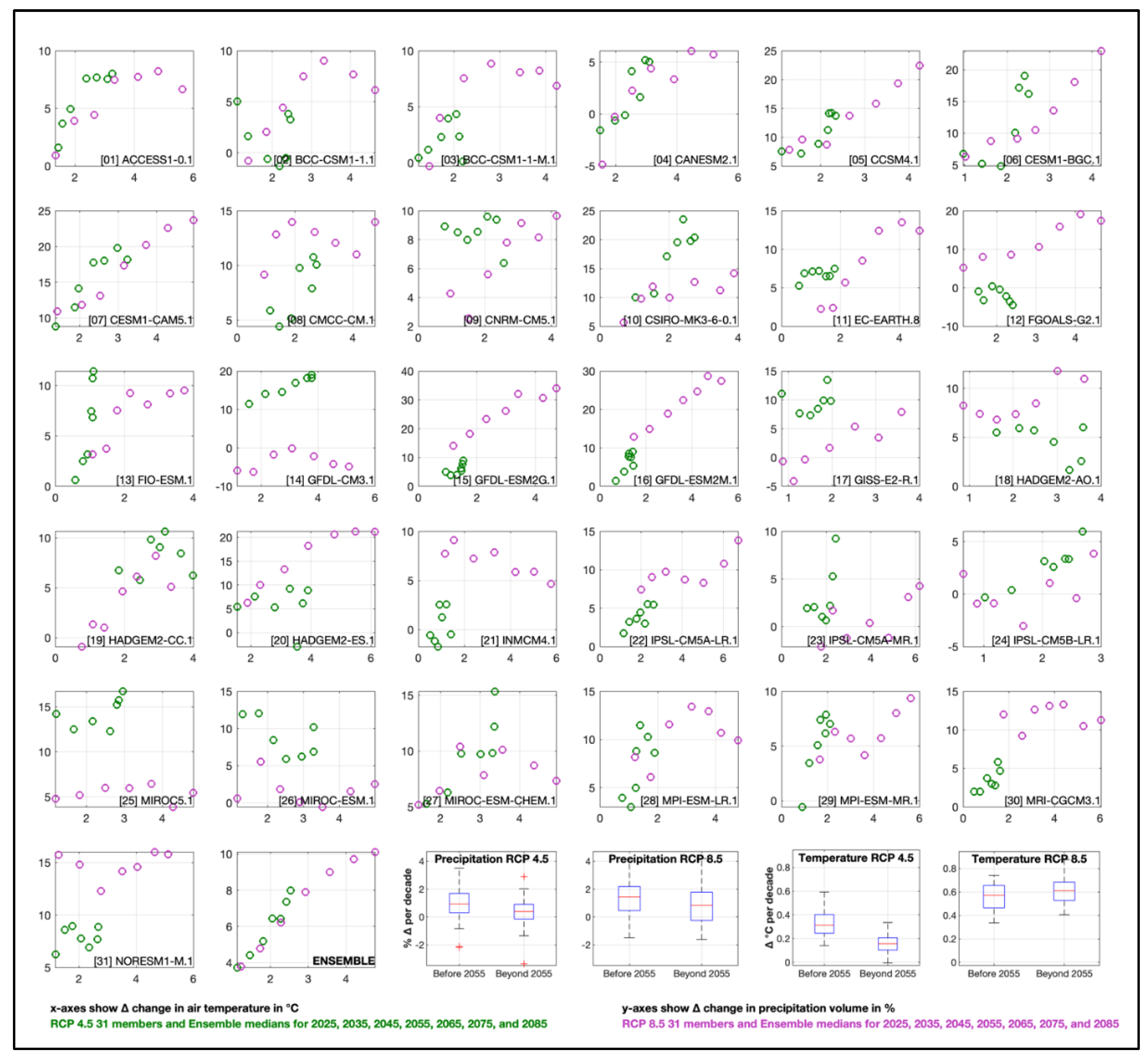
Figure A2.
Change in precipitation and air temperature over the Chesapeake Bay Watershed based on the MACA (Multivariate Adaptive Constructed Analogs) downscaling product from The Climatology Lab of John Abatzoglou. The MACA method (Abatzoglou, 2013) was applied to the output of 20 GCMs from the fifth phase of the Coupled Model Intercomparison Project (CMIP5) run under historical radiative forcing until 2005 and then for the RCP 4.5 and 8.5 scenarios until 2100. Shown are median changes in 30-year averages centered on 2025, 2035, 2045, 2055, 2065, 2075, and 2085 as compared to 1995.
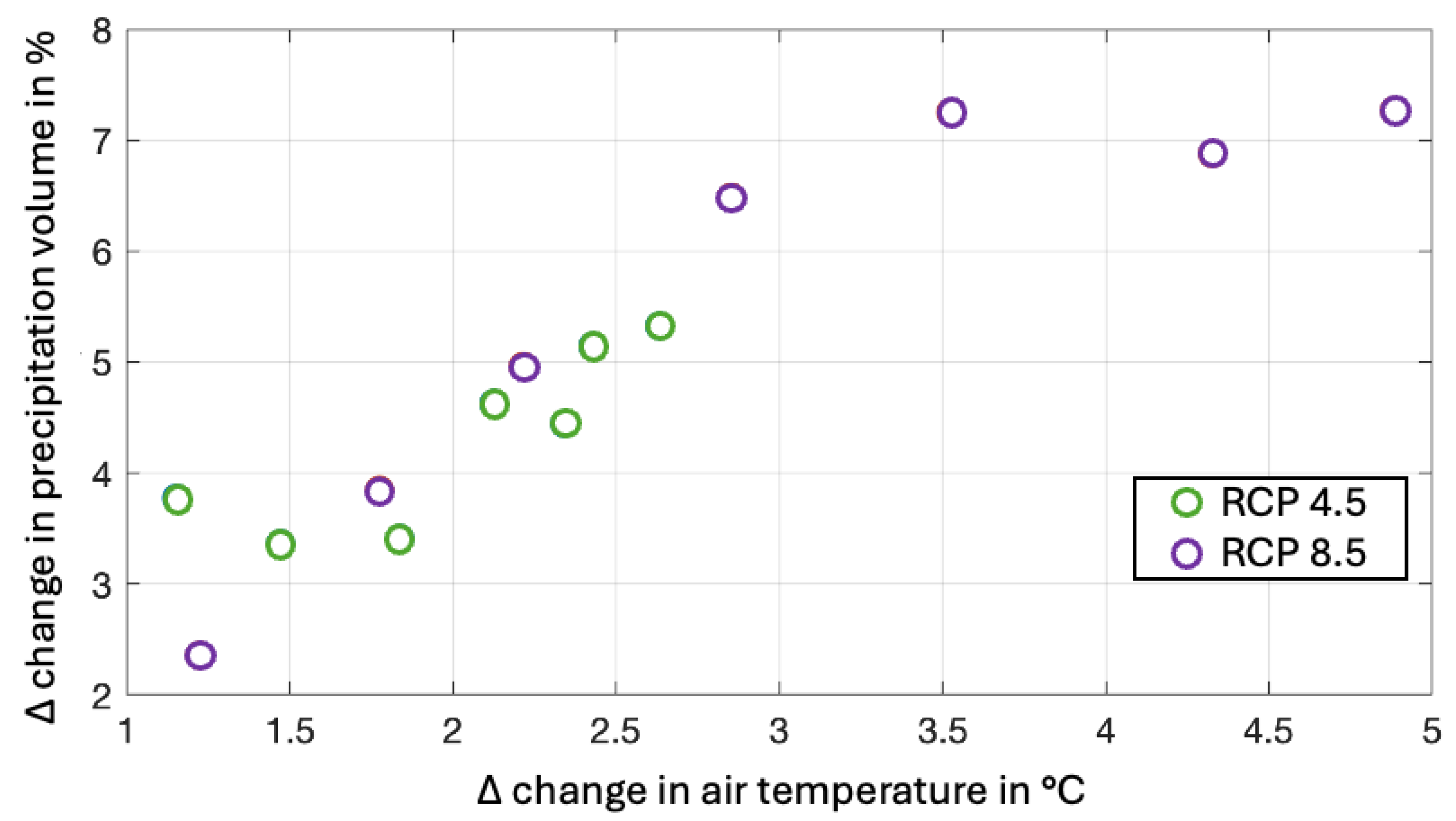
Figure A3.
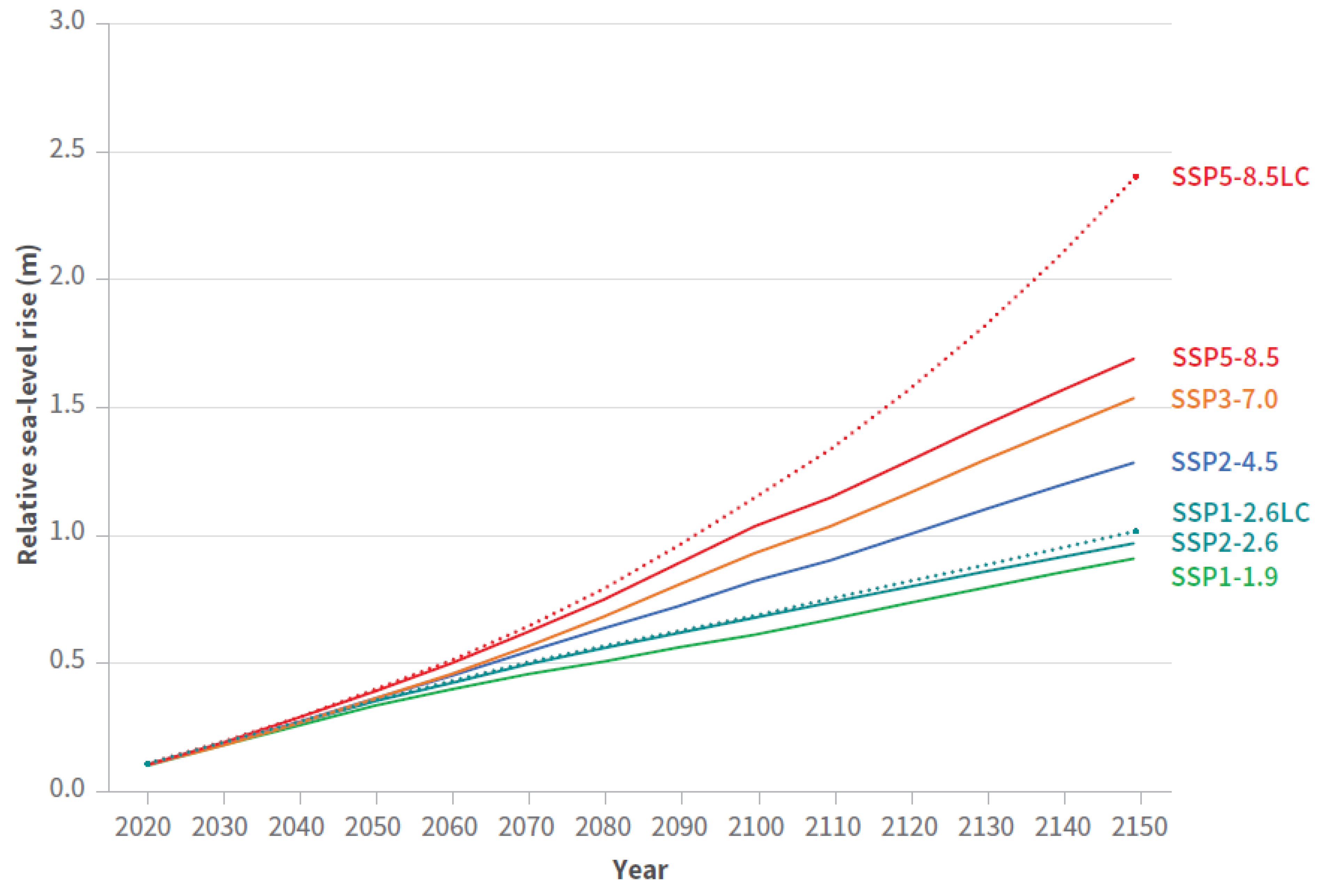
Estimated median sea level rise projections at Baltimore under emissions scenarios included in the IPCC AR6. Source: Bosch et al. 2023; NASA Sea Level Projection Tool and Sea-Level Rise Projections for Maryland.
Figure A3.
Estimated median sea level rise projections at Baltimore under emissions scenarios included in the IPCC AR6. Source: Bosch et al. 2023; NASA Sea Level Projection Tool and Sea-Level Rise Projections for Maryland.
References
- Abatzoglou, J.T., 2013. Development of gridded surface meteorological data for ecological applications and modelling. International Journal of Climatology, 33(1): 121–131.
- Anandhi, A., Frei, A., Pierson, D.C., Schneiderman, E.M., Zion, M.S., Lounsbury, D. and Matonse, A.H., 2011. Examination of change factor methodologies for climate change impact assessment. Water Resources Research 47:3.
- Basenback, N., J.M. Testa, and C. Shen, 2021. Warming and nutrient load timing effects on the phenology of Chesapeake Bay hypoxia. Journal of the American Water Resources Association.
- Bureau of Reclamation. 2013. Downscaled CMIP3 and CMIP5 Climate Projections: Release of Downscaled CMIP5 Climate Projections, Comparison with Preceding Information, and Summary of User Needs. iv Downscaled CMIP3 and CMIP5 Climate and Hydrology Projections. Denver, CO: U.S. Department of the Interior, Bureau of Reclamation, Technical Service, Center.
- Bhatt, G., L.C. Linker, G.W. Shenk, I. Bertani, R. Tian, J. Rigelman, K. Hinson, and P. Claggett, 2023. Water Quality Impacts of Climate Change, Land Use, and Population Growth in the Chesapeake Bay Watershed. Journal of the American Water Resources Association (JAWRA) J Am Water Resour Assoc. 2023;59:1313–1341.
- Boesch, D. F., Baecher, G. B., Boicourt, W. C., Cullather, R. I., Dangendorf, S., Henderson, G. R., Kilbourne, H. H., Kirwan, M. L., Kopp, R. E., Land, S., Li, M., McClure., K., Nardin, W., & Sweet, W. V. 2023. Sea-level Rise Projections for Maryland 2023. University of Maryland Center for Environmental Science, Cambridge, MD. (https://www. umces.edu/sea-level-rise-projections).
- Boon, J.D. and M. Mitchell, 2015. Nonlinear Change in Sea Level Observed at North American Tide Stations. Journal of Coastal Research (2015) 31 (6): 1295–1305. Accessed September 18, 2021. [CrossRef]
- Bormann, H., 2011. Sensitivity analysis of 18 different potential evapotranspiration models to observed climatic change at German climate stations. Climatic Change, 104(3), 729-753.
- Boynton, R.W., J.H. Garber, R. Summers, and W.M. Kemp, 1995. Inputs, Transformations, and Transport of Nitrogen and Phosphorus in Chesapeake Bay and Selected Tributaries. Estuaries 18(1B):285-314.
- Boynton, W.R. and W.M. Kemp, 2008. Estuaries. In: Nitrogen in the Marine Environment (Second Edition), D.G. Capone, D.A. Bronk, M.R. Mulholland, and E.J. Carpenter (Editors). Elsevier Inc., Burlington, Massachusetts, pp. 809-866.
- Cai, X., J. Shen, Y.J. Zhang, Q. Qin, Z. Wang, and H. Wang, 2021. Impacts of Sea-Level Rise on Hypoxia and Phytoplankton Production in Chesapeake Bay: Model Prediction and Assessment. Journal of the American Water Resources Association 1–18. Accessed August 7, 2021. [CrossRef]
- Campbell, P.C., J.O. Bash, C.G. Nolte, T.L. Spero, E.J Cooter, K. Hinson, and L.C. Linker, 2019. Projections of Atmospheric Nitrogen Deposition to the Chesapeake Bay Watershed. Journal of Geophysical Research: Biogeosciences, 124. Accessed August 7, 2021. [CrossRef]
- Cerco, C.F. and M.R. Noel, 2004. The 2002 Chesapeake Bay Eutrophication Model. EPA 903-R-04-004, U.S. Environmental Protection Agency, Chesapeake Bay Program Office, Annapolis, Maryland.
- Cerco, C.F., S.C. Kim, and M.R. Noel, 2010. The 2010 Chesapeake Bay Eutrophication Model. A Report to the US Environmental Protection Agency and to the US Army Corps of Engineer Baltimore District. US Army Engineer Research and Development Center, Vicksburg, Mississippi. http://www.chesapeakebay.net/publications/title/the_2010_chesapeake_bay_eutrophication_model1 Accessed April 2022.
- Cerco, C.F and M.R. Noel, 2019. Chesapeake Bay Water Quality and Sediment Transport Model Chesapeake Bay Program Office December 2019 Final Report. Annapolis, MD. 580 pages. https://www.chesapeakebay.net/channel_files/28679/2017_chesapeake_bay_water_quality_and_sediment_transport_model.pdf Accessed September 1, 2021.
- CBPO (Chesapeake Bay Program Office), 2020. Phase 6 Dynamic Watershed Model and CAST-17 Documentation. https://cast.chesapeakebay.net/Documentation/ModelDocumentation Accessed May 5, 2023.
- Daly, C., M. Halbleib, J.I. Smith, W.P. Gibson, M.K. Doggett, G.H. Taylor, J. Curtis, and P.P. Pasteris, 2008. Physiographically sensitive mapping of climatological temperature and precipitation across the conterminous United States. International Journal of Climatology: a Journal of the Royal Meteorological Society 28, no. 15: 2031-2064.
- de Castro, M., C. Gallardo, and K. Jylha, 2007. The use of a climate-type classification for assessing climate change effects in Europe from an ensemble of nine regional climate models. Climatic Change 81, 329–341. [CrossRef]
- Fox-Kemper, B., H.T. Hewitt, C. Xiao, G. Aðalgeirsdóttir, S.S. Drijfhout, T.L. Edwards, N.R. Golledge, M. Hemer, R.E. Kopp, G. Krinner, A. Mix, D. Notz, S. Nowicki, I.S. Nurhati, L. Ruiz, J.-B. Sallée, A.B.A. Slangen, and Y. Yu, 2021: Ocean, Cryosphere and Sea Level Change. In Climate Change 2021: The Physical Science Basis. Contribution of Working Group I to the Sixth Assessment Report of the Intergovernmental Panel on Climate Change [Masson-Delmotte, V., P. Zhai, A. Pirani, S.L. Connors, C. Péan, S. Berger, N. Caud, Y. Chen, L. Goldfarb, M.I. Gomis, M. Huang, K. Leitzell, E. Lonnoy, J.B.R. Matthews, T.K. Maycock, T. Waterfield, O. Yelekçi, R. Yu, and B. Zhou (eds.)]. Cambridge University Press, Cambridge, United Kingdom and New York, NY, USA, pp. 1211–1362, . [CrossRef]
- Hamon, W.R., 1961. Estimating potential evapotranspiration. Journal of the Hydraulics Division ASCE, 87(3): 107-120.
- Hargreaves, G. H., and Z.A. Samani, 1985. Reference crop evapotranspiration from temperature. Applied Engineering in Agriculture, 1(2), 96-99.
- Hausfather, Z., and G.P. Peters, 2020a. Emissions–the ‘business as usual’ story is misleading. Nature 577: 618-620.
- Hausfather, Z., and G.P. Peters, 2020b. RCP8.5 is a problematic scenario for near-term emissions." Proceedings of the National Academy of Sciences 117:45 27791-27792.
- Hood, R.R., G.W. Shenk, R.L. Dixon, S.M.C. Smith, W.P. Ball, J.O. Bash, R. Batiuk, K. Boomer, D.C. Brady, C.F. Cerco, P. Claggett, K. de Mutsert, Z.M. Easton, A.J. Elmore, M.A.M. Friedrichs, L. Harris, T.F. Ihde, I. Lacher, L. Li, L.C. Linker, A. Miller, J. Moriarty, G. Noe, G. Onyullo, K. Rose, K. Skalak, R. Tian, T.L. Veith, L. Wainger, D. Weller, Y. J. Zhang, 2021. The Chesapeake Bay Program Modeling System: Overview and Recommendations for Future Development. Ecological Modelling 456 (2021) 109635 Accessed August 7, 2020. [CrossRef]
- IPCC, 2013: Climate Change 2013: The Physical Science Basis. Contribution of Working Group I to the Fifth Assessment Report of the Intergovernmental Panel on Climate Change [Stocker, T.F., D. Qin, G.-K. Plattner, M. Tignor, S.K. Allen, J. Boschung, A. Nauels, Y. Xia, V. Bex and P.M. Midgley (eds.)]. Cambridge University Press, Cambridge, United Kingdom and New York, NY, USA, 1535 pp.
- IPCC, 2014: Climate Change 2014: Synthesis Report. Contribution of Working Groups I, II and III to the Fifth Assessment Report of the Intergovernmental Panel on Climate Change [Core Writing Team, R.K. Pachauri and L.A. Meyer (eds.)]. IPCC, Geneva, Switzerland, 151 pp.
- Irby, I.D., M.A.M. Friedrichs, F. Da, and K.E. Hinson, 2018. The Competing Impacts of Climate Change and Nutrient Reductions on Dissolved Oxygen in Chesapeake Bay. Biogeosciences, 15, 2649–2668, 2018 Accessed August 7, 2020. [CrossRef]
- Journal of American Water Resources Association (JAWRA) Featured Collection, 2013. Chesapeake Bay Total Maximum Daily Load Development and Application Eds. R.A Batiuk, L.C. Linker, and C.F. Cerco https://onlinelibrary.wiley.com/toc/17521688/2013/49/5 Accessed January 27, 2025.
- Journal of American Water Resources Association (JAWRA) Featured Collection, 2022. Influence of Climate Change on Chesapeake Bay Water Quality Eds. C.F. Cerco, L.C. Linker, G. Bhatt, and G.W. Shenk https://onlinelibrary.wiley.com/doi/toc/10.1111/(ISSN)1752-1688.chesapeake-bay Accessed January 27, 2025.
- Johnson, Z., M. Bennett, L.C. Linker, S. Julius, R. Najjar, M. Mitchell, D. Montali, R. Dixon. 2016. The Development of Climate Projections for Use in Chesapeake Bay Program Assessments. STAC Publication Number 16-006, Edgewater, MD. 52 pp. http://www.chesapeake.org/pubs/360_Johnson2016.pdf Accessed January 27, 2025.
- Karl, T.R. and Knight, R.W., 1998. Secular trends of precipitation amount, frequency, and intensity in the United States. Bulletin of the American Meteorological society, 79(2), pp.231-242.
- Kemp, W.M., P.A. Sampou, J.H. Garber, J. Tuttle, and W.R. Boynton, 1992. Seasonal Depletion of Oxygen from Bottom Waters of Chesapeake Bay: Roles of Benthic and Planktonic Respiration and Physical Exchange Processes. Marine Ecology Progress Series 85:137-152.
- Kemp, W.M., W.R Boynton, J.E. Adolf, D.F. Boesch, W.C. Boicourt, G. Brush, J.C. Cornwell, T.R. Fisher, P.M. Glibert, J.D. Hagy, L.W. Harding, E.D. Houde, D.G. Kimmel, W.D. Miller, R.E.I. Newell, M.R. Roman, E.M. Smith, J.C. Stevenson, 2005. Eutrophication of Chesapeake Bay: Historical trends and ecological interactions. Marine Ecology Progress Series 303, 1–29.
- Kingston, D. G., M. C. Todd, R.G. Taylor, J.R. Thompson, and N.W. Arnell, 2009. Uncertainty in the estimation of potential evapotranspiration under climate change. Geophysical Research Letters, 36(20).
- Kopp, R.E., R.M. Horton, C.M. Little, J.X. Mitrovica, M. Oppenheimer, D.J. Rasmussen, B.H. Strauss, and C. Tebaldi, 2014). Probabilistic 21st and 22ndcentury sea-level projections at a global network of tide-gauge sites, Earth’s Future, 2, 383–406, https://agupubs.onlinelibrary.wiley.com/doi/epdf/10.1002/2014EF000239. Accessed September 18, 2021. [CrossRef]
- Kutta, E. and J.A. Hubbart, 2018. Changing climatic averages and variance: Implications for mesophication at the eastern edge of North America’s Eastern deciduous forest. Forests 9(10), 605.
- Linker, L. C., R.A. Batiuk, G.W. Shenk, and C.F. Cerco, 2013. Development of the Chesapeake Bay Watershed Total Maximum Daily Load Allocation. Journal of the American Water Resources Association (JAWRA) 49(5): 986-1006. [CrossRef]
- Linker, L.C., G.W. Shenk, G. Bhatt, R. Tian, C.F. Cerco, and I. Bertani, 2023. Simulating climate change in a coastal watershed with an integrated suite of airshed, watershed, and estuary models. Journal of the American Water Resources Association (JAWRA) 60(2): 499-528. [CrossRef]
- Maurer, E.P., L. Brekke, T. Pruitt, and P.B. Duffy. 2007. “Fine-Resolution Climate Projections Enhance Regional Climate Change Impact Studies.” EOS Transactions 88(47): 504.
- Melillo, Jerry M., Terese (T.C.) Richmond, and Gary W. Yohe, Eds., 2014: Climate Change Impacts in the United States: The Third National Climate Assessment. U.S. Global Change Research Program, 841 pp. https://www.nrc.gov/docs/ML1412/ML14129A233.pdf. [CrossRef]
- Milly, P.C.D., J. Betancourt, M. Falkenmark, R.M. Hirsch, Z.W. Kundzewicz, D.P. Lettenmaier, R.J. Stouffer, 2008. Stationarity Is Dead: Whither Water Management? Science Vol 319 1 February 2008.
- Najjar, R., C. Pyke, M. Adams, D. Breitburg, C. Hershner, M. Kemp, R. Howarth, M. Mulholland, M. Mulholland, D. Secor, K. Sellner, D. Wardrop, and R. Woodman. 2010. Potential climate-change impacts on the Chesapeake Bay. Estuarine, Coastal and Shelf Science 86 (2010) 1–20.
- Paolisso, M., Trombley, J., Hood, R.R. et al., 2015. Environmental Models and Public Stakeholders in the Chesapeake Bay Watershed. Estuaries and Coasts 38, 97–113. [CrossRef]
- Pielke Jr, R., Burgess, M.G. and Ritchie, J., 2022. Plausible 2005-2050 emissions scenarios project between 2 and 3 degrees C of warming by 2100. Environmental Research Letters.
- Pyke, C.R., R.G. Najjar, M.B. Adams, D. Breitburg, M. Kemp, C. Hershner, R. Howarth, M. Mulholland, M. Paolisso, D. Secor, K. Sellner, D. Wardrop, and R. Wood. 2008. Climate Change and the Chesapeake Bay: State-of-the-Science Review and Recommendations. Chesapeake Bay Program Science and Technical Advisory Committee, Annapolis, MD. http://www.chesapeake.org/pubs/Pubs/climchangereport.pdf last accessed 4/2019.
- PSC (Principal’s Steering Committee), 2020. PSC Actions and Decisions of December 17, 2020 Meeting. Chesapeake Bay Program Office Annapolis, MD. https://www.chesapeakebay.net/channel_files/42484/draft_psc_actions-decisions_12-17-20_v5.pdf Accessed August 4, 2021.
- PSC (Principal’s Steering Committee), 2017. PSC Actions and Decisions of December 19-20, 2017 Meeting. Chesapeake Bay Program Office Annapolis, MD. https://www.chesapeakebay.net/channel_files/26045/dec_19 20_2917_cbp_psc_mtg_summary_of_actions_and_decisions_(3).pdf Accessed August 4, 2021.
- Ramirez Villejas, J., Jarvis, A. 2010. Downscaling Global Circulation Model Outputs: The Delta Method Decision and Policy Analysis Working Paper No. 1. International Center for Tropical Agriculture (CIAT). Cali. CO. 18 p. https://hdl.handle.net/10568/90731 Accessed August 26, 2021.
- Rice, K.C., Douglas L. Moyer, and Aaron L. Mills, 2017. Riverine discharges to Chesapeake Bay: Analysis of long-term (1927 - 2014) records and implications for future flows in the Chesapeake Bay basin Journal of Environmental Management 204 (2017) 246-254.
- Romero-Lankao, P., J.B. Smith, D.J. Davidson, N.S. Diffenbaugh, P.L. Kinney, P. Kirshen, P. Kovacs, and L. Villers Ruiz, 2014: North America. In: Climate Change 2014: Impacts, Adaptation, and Vulnerability. Part B: Regional Aspects. Contribution of Working Group II to the Fifth Assessment Report of the Intergovernmental Panel on Climate Change [Barros, V.R., C.B. Field, D.J. Dokken, M.D. Mastrandrea, K.J. Mach, T.E. Bilir, M. Chatterjee, K.L. Ebi, Y.O. Estrada, R.C. Genova, B. Girma, E.S. Kissel, A.N. Levy, S. MacCracken, P.R. Mastrandrea, and L.L. White (eds.)]. Cambridge University Press, Cambridge, United Kingdom and New York, NY, USA, pp. 1439-1498 https://www.ipcc.ch/site/assets/uploads/2018/02/WGIIAR5-Chap26_FINAL.pdf Accessed December 20, 2021.
- Schwalm, C.R., Glendon, S. and Duffy, P.B., 2020. RCP8.5 tracks cumulative CO2 emissions. Proceedings of the National Academy of Sciences, 117(33): 19656–19657.
- St-Laurent, P., M.A.M. Friedrichs, M. Li, and W. Ni. 2019. “Impacts of Sea Level Rise on Hypoxia in Chesapeake Bay: A Model Intercomparison.” Virginia Institute of Marine Science, William & Mary. Report to Virginia Tech and Chesapeake Bay Program, October 2019, 34 pp. https://scholarworks.wm.edu/reports/2310/ . [CrossRef]
- Shenk, G., M. Bennett, D. Boesch, L. Currey, M. Friedrichs, M. Herrmann, R. Hood, T. Johnson, L. Linker, A. Miller, and D. Montali. 2021a. Chesapeake Bay Program Climate Change Modeling 2.0 Workshop. STAC Publication Number 21-003, Edgewater, MD. 35 pp. https://www.chesapeake.org/stac/wp-content/uploads/2021/07/Final_STAC-Report-Climate-Change_7.22.2021.pdf.
- Shenk, G. W., Bhatt, G., Tian, R., Cerco, C.F., Bertani, I., Linker, L.C., 2021b. Modeling Climate Change Effects on Chesapeake Water Quality Standards and Development of 2025 Planning Targets to Address Climate Change. CBPO Publication Number 328-21, Annapolis, MD. 145 pp. https://cast-content.chesapeakebay.net/documents/P6ModelDocumentation%2FClimateChangeDocumentation.pdf Accessed October 15, 2022>.
- Shenk, Gary W. and Lewis C. Linker, 2013. Development and Application of the 2010 Chesapeake Bay Watershed Total Maximum Daily Load Model. Journal of the American Water Resources Association (JAWRA)49(5): 1042-1056. Accessed August 26, 2021. [CrossRef]
- Sinha, E., Michalak, A.M. and Balaji, V., 2017. Eutrophication will increase during the 21st century as a result of precipitation changes. Science, 357(6349), pp.405-408.
- STAC (Chesapeake Bay Program’s Scientific and Technical Advisory Committee), 2011. Adapting to Climate Change in the Chesapeake Bay: A STAC workshop to monitor progress in addressing climate change across the Chesapeake Bay Watershed. STAC Workshop Report March 15, 2011. STAC Publication 12-001. Philadelphia, PA.
- Tian, R., Cerco, C.F., Bhatt, G., Linker, L.C. and Shenk, G.W., 2022. Mechanisms controlling climate warming impact on the occurrence of hypoxia in Chesapeake Bay. JAWRA Journal of the American Water Resources Association, 58(6), pp.855-875. Accessed January 23, 2025. [CrossRef]
- USEPA (U.S. Environmental Protection Agency), 2010. Chesapeake Bay Total Maximum Daily Load for Nitrogen, Phosphorus and Sediment. U.S. Environmental Protection Agency Chesapeake Bay Program Office, Annapolis MD. https://www.epa.gov/chesapeake-bay-tmdl/chesapeake-bay-tmdl-document Accessed March 12, 2022.
- USEPA (U.S. Environmental Protection Agency), 2017. Community Multiscale Air Quality Model Version 5.2. U.S. EPA Office of Research and Development. Retrieved from https://zenodo.org/record/1167892.
- Wang, Ping, L. Linker, H. Wang, G. Bhatt, G. Yactayo, K. Hinson, and R Tian, 2017. Assessing water quality of the Chesapeake Bay by the impact of sea level rise and warming. 3rd International Conference on Water Resource and Environment (WRE 2017) IOP Conf. Series: Earth and Environmental Science 82 (2017) 012001 . [CrossRef]
- https://www.researchgate.net/publication/319412153_Assessing_water_quality_of_the_Chesapeake_Bay_by_the_impact_of_sea_level_rise_and_warming#fullTextFileContent Accessed September 21, 2021.
Figure 1.
Effects of 2025 (Figure 1a) and 2085 (Figure 1b) estimated assessment of changing environmental conditions on the Chesapeake Bay and its watershed relative to the 1995 Chesapeake TMDL Reference Period.
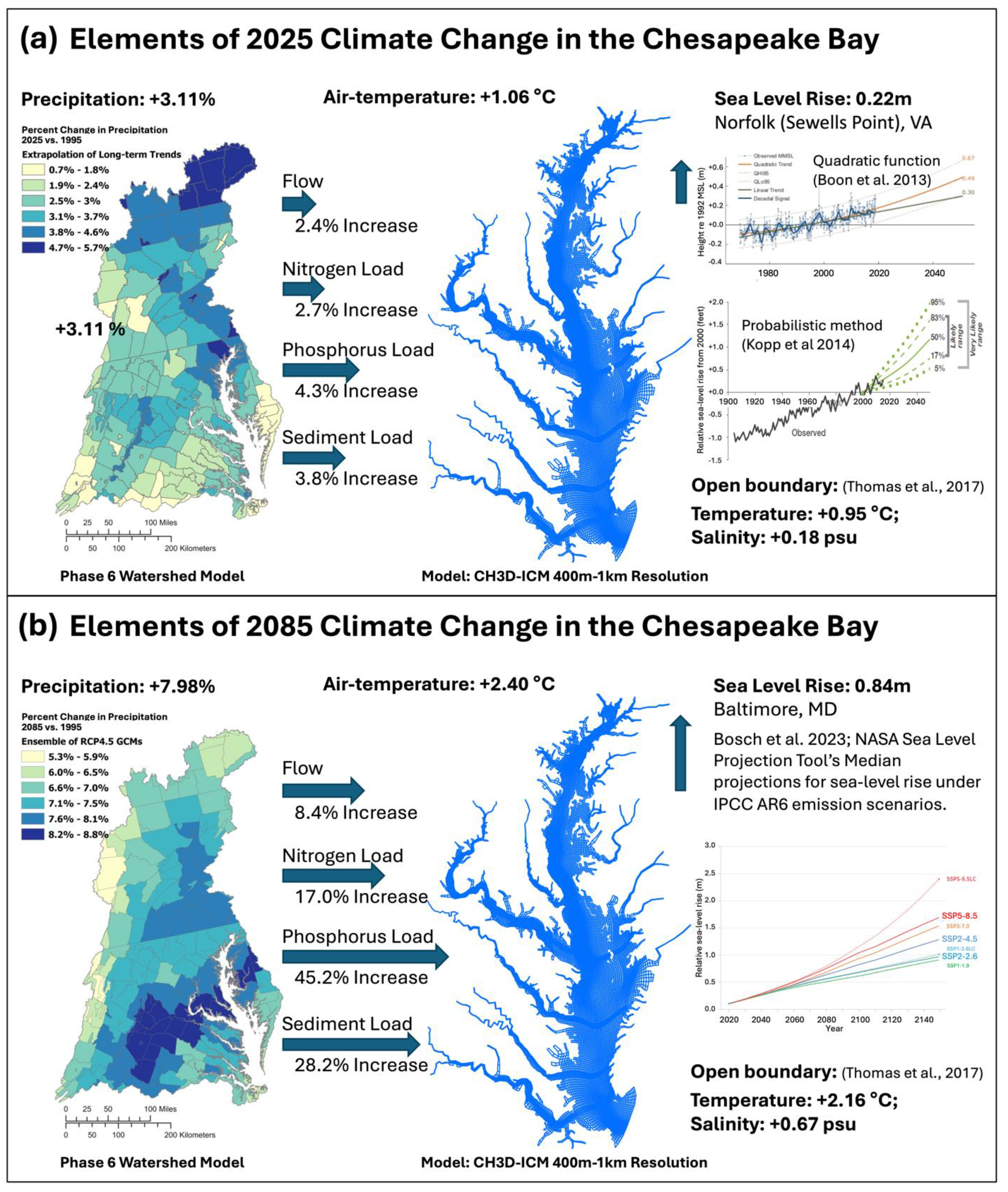
Figure 2.
Change in air temperature (2a) and precipitation (2b) relative to 1995 for the ensemble median of 31 statistically downscaled CMIP5 RCP 4.5 and RCP 8.5 scenarios. Prior assessment of changing environmental conditions for the years 2025, 2035, 2045, and 2055 were based on RCP 4.5 for air temperature, whereas change in precipitation was based on long-term observed trends for 2025, RCP 4.5 for 2055, and blend of the long-term trend and RCP 4.5 for 2035 and 2045 (Bhatt et al., 2023). This analysis for 2065, 2075, and 2085 considers ensemble median of both RCP 4.5 and RCP 8.5.
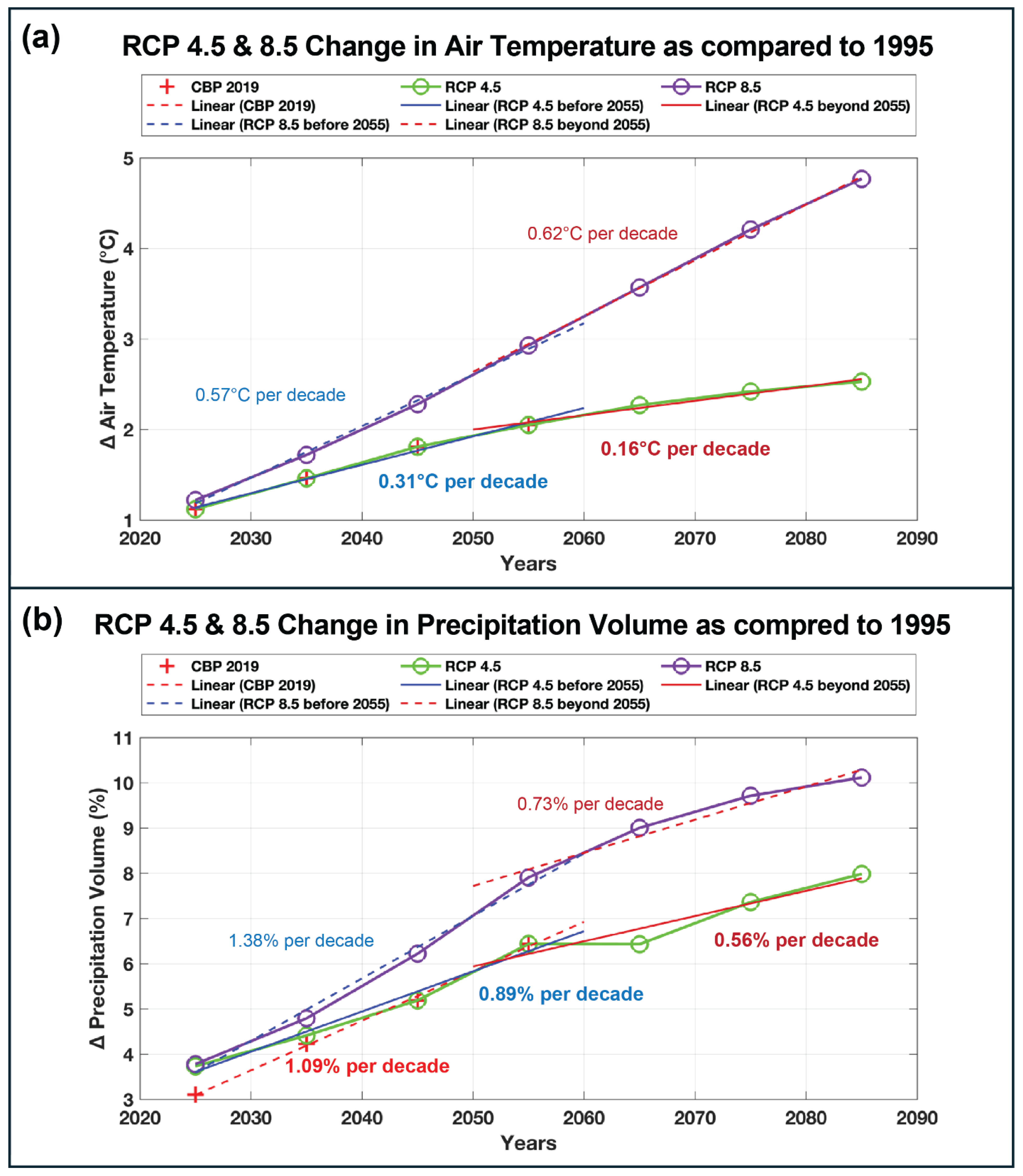
Figure 3.
Estimated hypoxia effects under 2025 Phase 3 WIP conditions (Blue bars) and 2085 Phase 3 WIP conditions (Red bars) with no environmental change effects (Reference), with the addition of environmental change watershed and airshed loads (Watershed Loads), with the addition of 2025 sea level rise (Sea Level Rise), with the addition of 2025 water-column warming (Warmer Water; D: Contribution of DO solubility to the total increase in hypoxia volume from the Reference scenario; R: Contribution of respiration to the total hypoxia volume increase; S: Contribution of stratification to the total increase of hypoxia volume increase), and with all three factors combined (All Together). Hypoxia volume (in km3) is the average in summer (June - September) from 1991 through 2000 in the whole Bay with DO concentration lower than 1 mg/L.
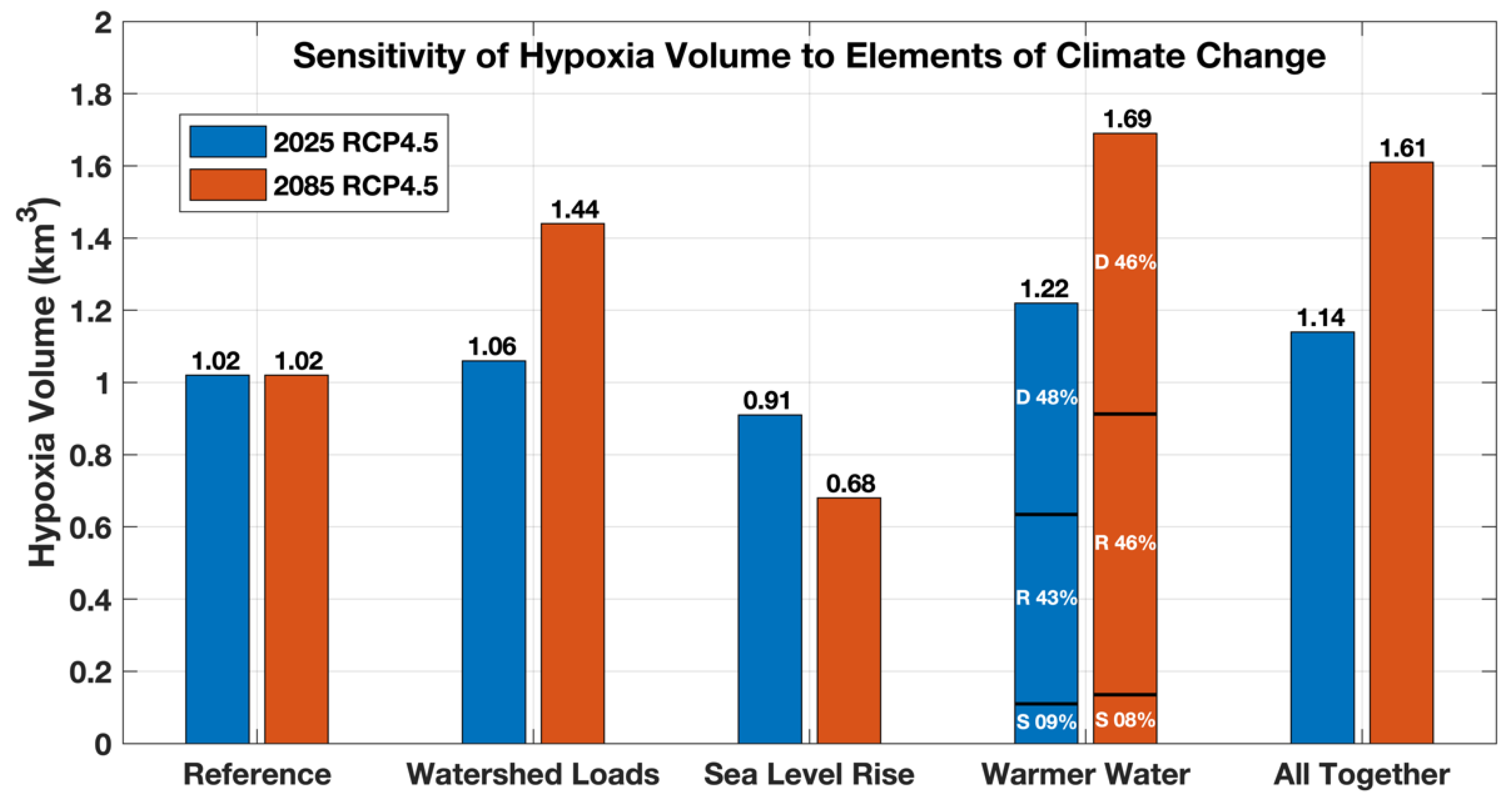
Figure 4.
Estimated Chesapeake hypoxia (June to September DO < 1.0 mg/l) for the decadal increments of environmental conditions from 2025 to 2085 all with the Phase 3 Chesapeake Watershed Implementation Plan (WIP3) under RCP 4.5 (green lines) and RCP 8.5 (purple lines). The hypoxia volume in the 1990s is for estimated watershed loads and Bay under the WIP3 conditions at the 1991-2000 base hydrology condition. Dashed lines with + markers are sea level rise, with x markers are nutrient load increase, triangle markers are temperature increase. Solid lines are the combined effect of sea level rise, nutrient load and temperature increases. The 2130 scenario kept all inputs the same as 2085 RCP 4.5 but the sea level rise changed to the 2130 level.
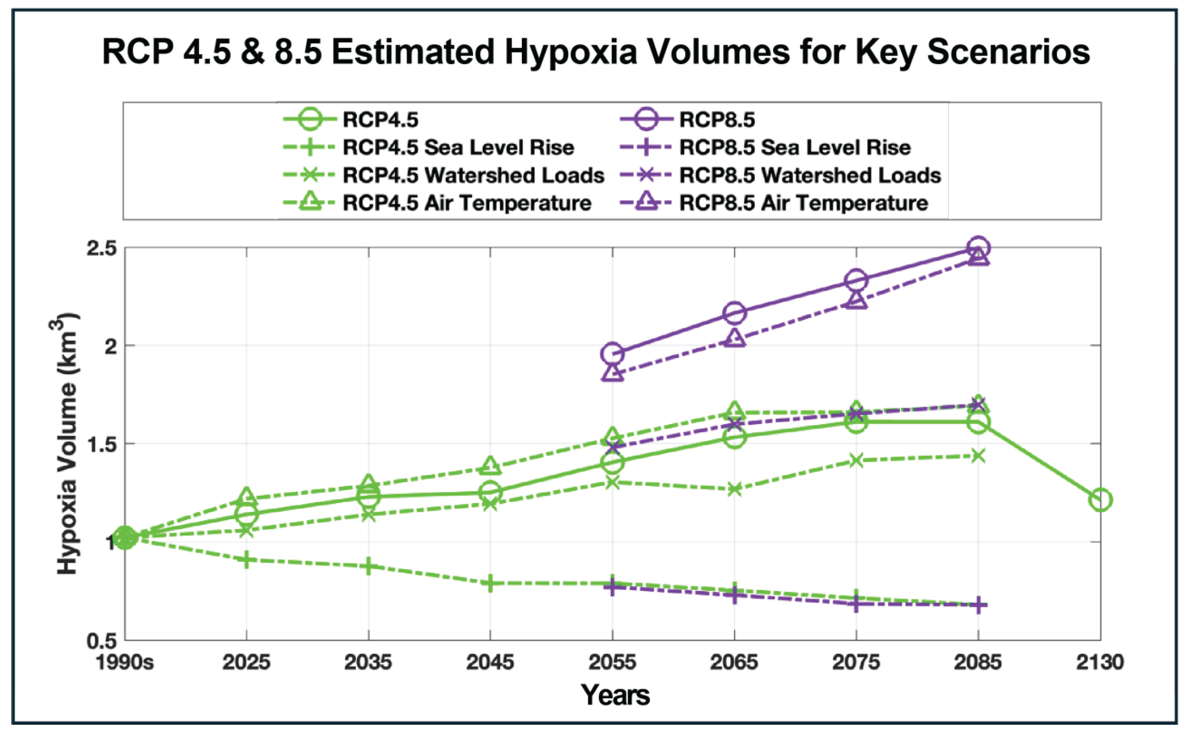
Figure 5.
Global CO2 emission estimates (adapted from Hausfather and Peters, 2020a. Nature) and estimated regional responses of total Chesapeake Bay hypoxia (June to September DO < 1.0 mg/l).
Figure 5.
Global CO2 emission estimates (adapted from Hausfather and Peters, 2020a. Nature) and estimated regional responses of total Chesapeake Bay hypoxia (June to September DO < 1.0 mg/l).
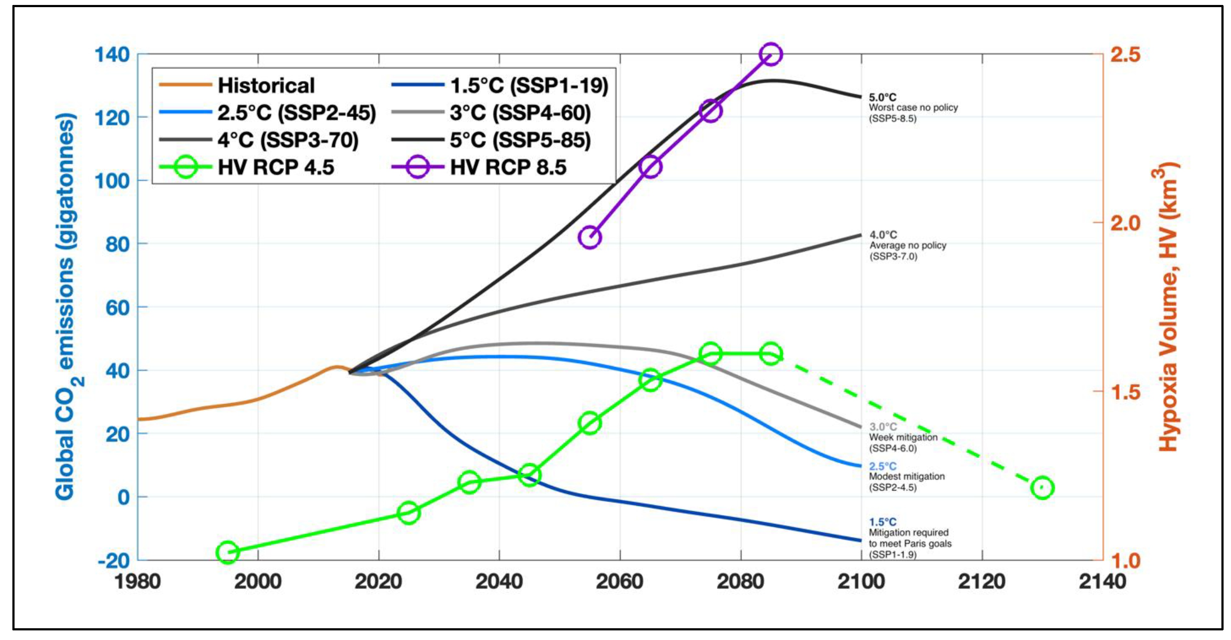

Table 1.
Watershed-wide estimated average change in precipitation (PRC), surface air temperature (TAS), streamflow (Flow), loads of nitrogen (TN Load), phosphorus (TP Load), in millions of kg, and suspended sediment (SS Load) in billions of kg delivered to the Chesapeake Bay for 2025 to 2085 with respect to 1995 Reference Period. The RCP 4.5 and RCP 8.5 indicate that the ensemble median of 31 statistically downscale GCMs were used. Hybrid indicates a combination of precipitation trends and ensemble medians were used as described in Bhatt et al. (2023). The 2025 to 2055 results were previously described in Linker et al. (2023). 1991–2000 base hydrology and conditions* were used for all scenarios and had average estimated annual rainfall of 105.6 cm, streamflow of 44.8 cm, nitrogen load of 90.3 million kg, phosphorus load of 6.09 million kg, and sediment load of 8.43 billion kg.
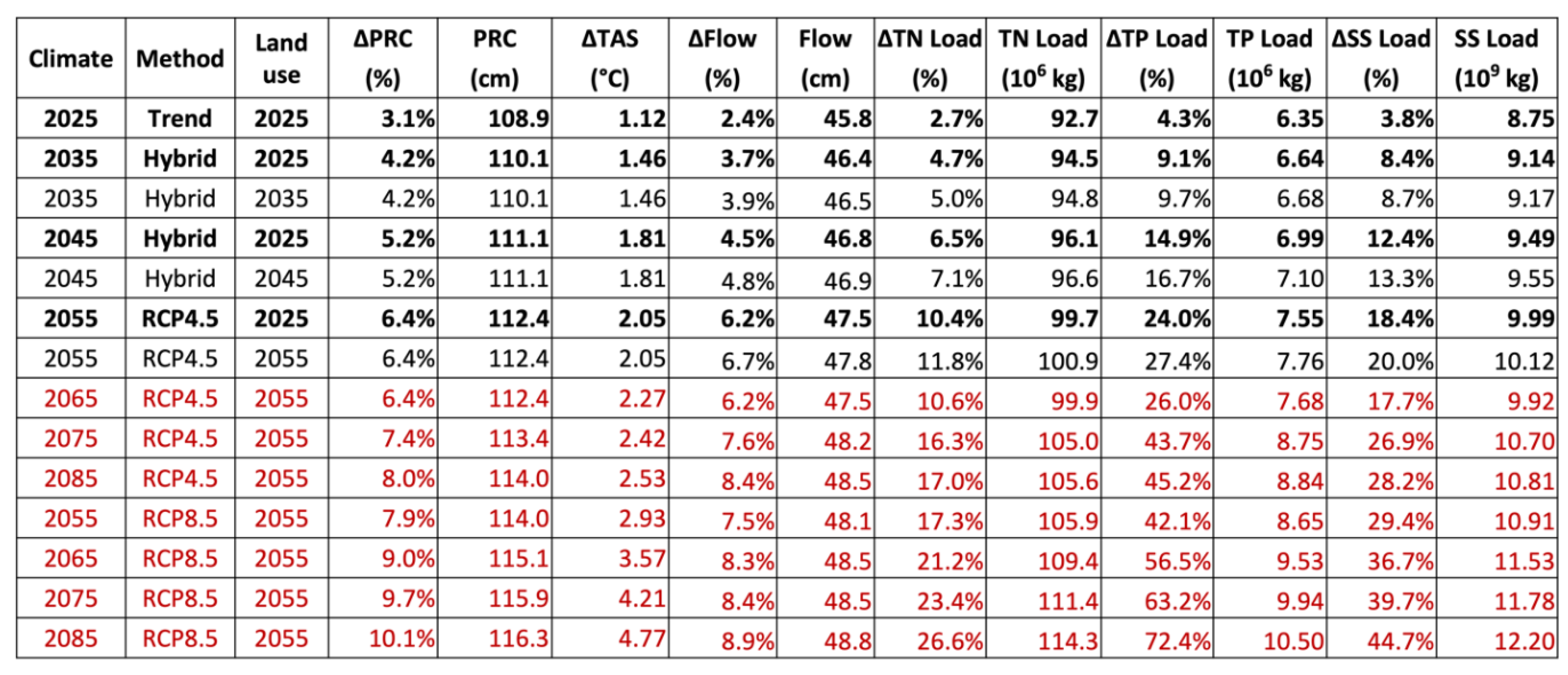 |
* The 1995 Reference Period, also called the 1991-2000 Planning Target Level of Effort Scenario (PT-LOE), was used as a base condition in all scenarios. The PT-LOE conditions represent the loads required to achieve water quality standards under the Chesapeake TMDL (apart from changing environmental conditions) and closely approximate the final Watershed Implementation Plan Phase 3 loads that were put forward by the CBP partnership.
Disclaimer/Publisher’s Note: The statements, opinions and data contained in all publications are solely those of the individual author(s) and contributor(s) and not of MDPI and/or the editor(s). MDPI and/or the editor(s) disclaim responsibility for any injury to people or property resulting from any ideas, methods, instructions or products referred to in the content. |
© 2026 by the authors. Licensee MDPI, Basel, Switzerland. This article is an open access article distributed under the terms and conditions of the Creative Commons Attribution (CC BY) license (http://creativecommons.org/licenses/by/4.0/).
Copyright: This open access article is published under a Creative Commons CC BY 4.0 license, which permit the free download, distribution, and reuse, provided that the author and preprint are cited in any reuse.


