Submitted:
30 January 2026
Posted:
02 February 2026
You are already at the latest version
Abstract
Being either true or false, 1 or 0, the standard logic and the Boolean algebra traditionality never rotate. Thus, it can only account for polarization states but not superposition states. This paper proves the Boolean rotation theorem through complexifications. This result allows us to formulate polarization spinors as well as superpositions spinors. It provides a new understanding of the Riemann sphere of two-state systems. It also provides an alternative solution to the measurement of wavefunctions, which accounts for both the U-process and the R-process. The work reported in this paper formulates the Penrose twistor geometry of the polarization spinors and the superposition spinors.
Keywords:
Boolean algebra
; complexification
; rotation theorem
; polarization
; superposition
; spinor
; twistor
; Riemann sphere
; wavefunction
; stochastic sampling
1. Introduction
Let’s pay attention to three things. First, the standard logic and the Boolean algebra traditionality never rotate; thus, it can only account for polarization states but not superposition states. Second, superposition states happen in many scientific domains such as in mathematics and theoretical physics. Third, as David Hilbert stated at the Second World Congress of Mathematicians (1900), the modern mathematics needs a logically consistent foundation. Gödel’s independent result (1931) did not meet the Hilbert expectation. This incredibly uncomfortable situation has been ongoing for more than a century and needs to be improved. Our approach to improve this situation is to change logic, namely, to let logic rotate. The question is how.
In this paper, we first prove the Boolean rotation theorem through complexifications. This result allows to formulate polarization spinors as well as superpositions spinors. It provides a new understanding of the Riemann sphere of two-state systems. It also provides an alternative solution of the measurement problem of wavefunction, which accounts for both the U-process and the R-process. This work formulates the Penrose twistor geometry of the polarization spinors and the superposition spinors.
The contents of the rest part of this paper are as follows.
§2. Logic Rotations as Spinors. 2.1 The gap between logic and mathematics. 2.2 Complexification and logic rotation. 2.3 The Boolean Weyl-spinor. 2.4 The Boolean Dirac-Spinor and superpositions. 2.5 The Boolean Penrose-twistor.
§3. Projection to Riemann Sphere of Two-Sate Systems. 3.1 Polarizations and analytic continuations. 3.2 Möbius transformation and Riemann sphere. 3.3 Metalogic charge and Boolean superpositions.
§4. Geometry of Wavefunctions. 4.1 Wavefunction as a dual-process. 4.2 The R-process and the Yes/No measurement. 4.3 Projections as polarizations. 4.4 Stochastic sampling. 4.5 Geometry of the wavefunction.
§5. Concluding Remarks.
2. Logic Rotations as Spinors
2.1. The gap between logic and mathematics
There is a gap between logic and mathematics. Consider two logical operators: the conjunction (denoted as ) and disjunction (denoted as ); also consider two mathematical operations: addition (denoted as ) and multiplication (denoted as ). We demonstrate that the pair of logical operators and the pair of mathematical operations are not exchangeable. This can be seen from the following four possible cases.
Case 1 (conjunction and multiplication). (P); .
Case 2 (conjunction and addition). (P) and ((P). However, though , but .
Case 3 (disjunction and multiplication). (P) and ((P). However, though , but .
Case 4. (disjunction and addition). (P), but .
The above analyses show that logic unit elements and the negation are different from mathematical operations and inversions. Note that the truth-semantics and Boolean algebra are equivalent and the latter is the base of the digital language. Hence, the above distinction is not only the gap between logic and mathematics but also the distinction between digital language (i.e., computer science) and mathematical language.
2.2. Complexification and logic rotation
Consider the logic unite elements (0,1) in Boolean algebra. Let and .
Definition 2.1 (complexification).
and (2.1)
Their complex conjugates are
and , respectively (2.2)
Theorem 2.1 (modulus rotation). and . (2.3)
Proof. We have:
and
.
Corollary 2.1 By Definition 2.1 and Theorem 2.1, we observe that the complexifications and modulus computations cause the rotation of the unit elements in Boolean algebra. Call the rotation of this kind the Boolean rotation.
2.3. The Boolean Weyl-spinor
Similar to the Weyl spinor in quantum field theory, by Boolean rotation, we have
Definition 2.2 (Boolean Weyl-spinor). By the Definition 2.1, the Boolean spinor consists two complex components:
(2.4)
Which forms a two-component internal space. Its rotation satisfies the following four properties:
Property 1. Similar to the Weyl spinor, the Boolean spinor is polarized. It has only two spin directions, spin (up) or else spin (down); there are no superposition states between and . Hence, it spins .
Property 2. We know that the equation of the Weyl spinor characterizes massless and spin particles. The massless particles travel in the speed of light; this is the reflection of special relativity. The physical background of the Weyl spinor is the neutrino physics. There are no coupling operations are involved here; hence the Boolean spinor can be treated as ‘massless’, by which it means that pure logical rotation is contentless.
Property 3. Spin reflects the momentum of rotation. Helicity is the proper property of the Weyl spinor as well as the Boolean Weyl-spinor, which can be either left-handed or the right-handed. Because the massless particle travels in the speed of light, there is no distinctions between spin and helicity, which means we may treat the spin up () as the left-handed (L) and the spin down (as the right-handed (R) without loss of generality.
Property 4. Spinors change the sign after a circle of the rotation. In mathematics, by the sign-change it means to add the minus sign to a formula. Note that logic negation is different. Boolean algebra has only two elements, 0 and 1; i.e., and . Thus, by Theorem 2.1, the Boolean Weyl-spinor satisfies the sign-change condition.
To summarize, we have
Postulate 2.1. The Boolean Weyl-spinor is only committed to polarization states and .
2.4. The Boolean Dirac-Spinor and superpositions
The basic level of logical analysis is the propositional logic. A logic is a formal system, which is described by a formal language. It consists of the formal syntax and the formal semantics as standard components. The semantics of propositional logic is the truth-semantics. In logic, the only logical meaning is the truth-value, being either true (T) or false (F). The truth semantics is represented by the well-known truth table. To define T as 1 and F as 0, the truth-table becomes the Boolean algebra. Boolean algebra is the structure of the digital language. It is the starting point and the foundation of computer science.
Here, it is worth mentioning two non-standard logics. First, in standard logic, it commits to the law of excluded middle, which is formally represented as . But the intuitionistic logic does not admit this law. For the intuitive logic, and need to be independently constructed respectively. Second, by the fuzzy logic, it allows the truth-value to be any real numbers ranging from 0 to 1.
Definition 2.3 (Boolean Dirac-spinor). Consider two Boolean Weyl-spinors as follows:
, ; (2.5)
To couple up and , we define the Boolean Dirac-spinor below,
. (2.6)
This treatment is similar to the construction of the Dirac spinor in spinor field theory. Dirac spinor satisfies three properties.
Property 1. Coupling constant as mass and electric charge.
Property 2. It represents the massive and spin half particles (electron and positron). Because it is massive, by relativity, it is travels slower than the speed of light.
Property 3. It has no clear helicity and thus, it allows superposition states.
To extend these properties as the line of inferences, we have
Postulate 2.2 (superpositions). The Boolean Dirac-spinor is committed to superposition states of and .
2.5. The Boolean Penrose-twistor
The philosophy of twister theory has three core ideas. First: it holds a principle of composibility and assembling. In other words, for the twistor theory, the twistor space can be assembled but not a priori. Second: its building blocks at the bottom are lines but not points. Third: the principle of shortest path, which means the straight lines, such as light rays or geodesics are fundamental. As
The philosophy of twister theory has three core ideas. First: it holds a principle of composibility and assembling. In other words, for the twistor theory, the twistor space can be assembled but not a priori. Second: its building blocks at the bottom are lines but not points. Third: the principle of shortest path, which means the straight lines, such as light rays or null geodesics are fundamental. As Penrose characterized (2004), “Light rays as twistors”. Accordingly, the mathematical twistor equation is a line equation, which has two formats, the differential format and the integration format.
Definition 2.4 The integration format of the twistor equation is as follows
This is a straight-line equation, where serves as the slope and the intercept. Thus, a twistor is composed by two spinors:
The twistor space T, the vector space of solutions to the formula above, is a four-dimensional complex vector space and may be coordinatized with respect to a choice of origin, by a pair of spinors. We can see from (2.2) that a twistor is a four-dimensional complex vector .
Definition 2.5 (Boolean Penrose-twistor). Let be the Boolean Weyl-spinor (2.4) and the Boolean Dirac-spinor (2.6). Together they satisfy the twistor equation (2.7). Call this the Boolean Penrose twistor.
Postulate 2.3 The Boolean Penrose-twistor provides a unified account of both polarization and superposition states.
3. Projections to Riemann Sphere of Two-Sate Systems
The above discussions can be geometrically projected to the Riemann sphere of two-state system, which characterizes spin half particles (Penrose 2004). Here, spin means geometry. We do this in steps.
3.1. Polarizations and analytic continuations
Consider the Boolean Weyl-spinor defined in (2.4). We know the Weyl spinor is polarized without superposition states; thus, we may treat it as the pair of antipodes of the Riemann sphere of two-state system, denoted as .
Let us be a pair of metalogical monad and consider the spinor: validity vs invalidity. All the valid and invalid argument forms can be represented their unique Gödel numbers which are integers. As we know, the integer fields can be converted to complex fields through Riemann analytic continuation. We call those complex numbers the Gödel complex. We first define two categories as below:
Definition 3.1 The category that contains all of those Gödel complex as objects that represent valid argument forms. Plus, we introduce the monad A, called the validity monad, into the category which stands for the validity as a metaproperty. Thus, there is a morphism from A to each .
The above definition is a brief version, which demands some explanation next. Let denote the set of Gödel complexes that stand for valid argument forms. From this set, we construct a free (strict) symmetric monoidal category , using the tensor product and a unit object I. Within , there exists an object such that , indicating that is a monoid object in . This allows us to define an endofunctor, which satisfies the monad axioms. We refer as the validity monad. By the similar explanation, we have,
Definition 3.2 The category that contains all of those Gödel complex which represent the invalid argument forms. In addition, we introduce a monad , called the invalidity monad, into the category w. Thus, there is a morphism from each We then introduce two complex planes as follows.
Definition 3.3. The complex plane is with the zero-point , where is the validity monad defined by Definition 1.
Definition 3.4. The complex plane is with the zero-point , where is the invalidity monad defined by Definition 2.
3.2. Möbius transformation and Riemann sphere
We define the transformation from complex plane to as a holomorphic function : ; so that we have , which satisfies . The general transformation is as below:
where , so that the numerator is not a fixed multiple of the denominator. This is called a bilinear or Möbius transformation.
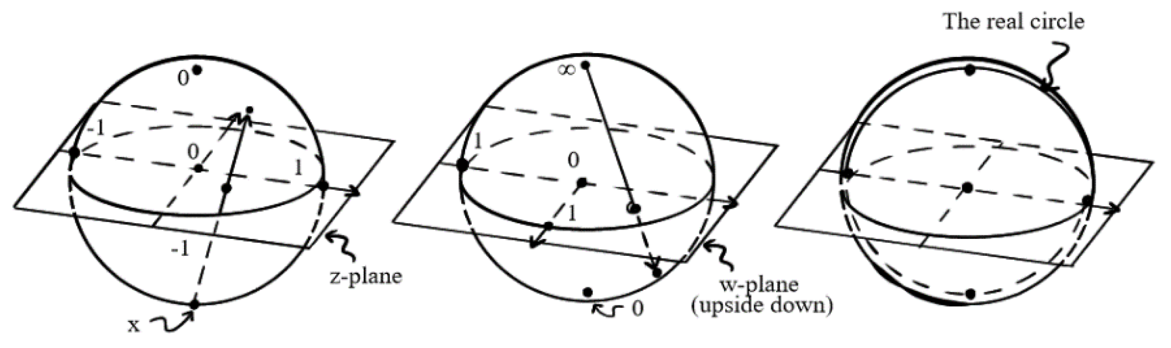
Note that the point removed from the -plane is that value which would give ‘’; correspondingly, the point removed from the w-plane is that value ( which would be achieved by ‘’. In fact, the whole transformation would make more global sense if we were to incorporate a quantity ‘’ into both the domain and target. This is one way of thinking about simplest (compact) Riemann surface of all: the Riemann sphere.
Now, we assume that a metalogic theory as a piece of mind has been divided into validity and invalidity based on the complex -plane and the w-plane respectively. The next step is to merge the complex planes into the so-called Riemann sphere of two-state systems. We regard the sphere as constructed from two ‘coordinate patches’: One of which is the -plane and the other the -plane. All but two points of the sphere are assigned both a -coordinate and a -coordinate (related by the Möbius transformation above). But one point has only -coordinate (where nd another has only w-coordinate (where We use , or both in order to define the needed conformal structure and, where we use both, we get the same conformal structure using either, because the relation between the two coordinates is holomorphic. In fact, for this, we do not need such a complicated transformation between and as the general Möbius transformation. It suffices to consider the particularly simple Möbius transformation given by
where and , would each give in the opposite patch. All this defines the Riemann sphere in a rather abstract way. See Penrose (2004, §8.3, pp.142-143) for further explanation.
Figure 1.
Riemann sphere from two complex planes.
The Riemann sphere above is called the conformal sphere, which puts validity and invalidity and in one system through metalogic. Here, we introduce another kind of Riemann sphere with more structures, which is called the metric sphere. This new Riemann sphere is a two-state system. The gauge field theoretic methods can be applied to make metalogic as a dynamic system.
Consider metalogical mind (like an electron) has an internal space. This internal space rotates. The mind possesses an intrinsic property called spin which is the momentum of its internal rotation. The metalogical mind-spin has two basic eigenstates: one is the validity monad and another is the invalidity monad, which are denoted as (called spin-up) and (spin-down), respectively. We assume the two eigenstates are orthogonal, and their linear superpositions are denoted by , which can be defined as follows,
where and are not just complex numbers but are amplitudes with certain Born probabilities. This is the reason why the corresponding Riemann sphere is a metric sphere that will be introduced shortly. The metalogical mind has an internal spin of , which is similar to an electron or quark. Each state has a complex phase. The difference between two state-phases yields new a phase (by linear superposition) called the dynamic or relative phase. For more detailed discussions, please see Penrose (2004, §22.9).
The above metalogic function of the two-state (the validity monad vs the invalidity monad) can be projected to the Riemann sphere of two-states. For the Riemann sphere with a two-state system, the key concept is the notion of antipodal points, which is part of the sphere’s structure. We use the north pole to represent the spin state . In the two-state metalogic function system, the north pole represents the validity monad and the south pole represents the invalidity monad , see Figure 2 below.
Suppose that the initial state of a two-state system is represented by the point B on the Riemann sphere and we wish to perform a Yes/No measurement corresponding to some other point on the sphere, where YES would find the state at A, and No would find it at the point , antipodal to A. If we take the sphere to have radius 1/2, and projecting B orthogonally to C on the axis , we find that the probability of YES is the length , which is and the probability of NO is the length CA, which is assuming that the angle is between OB and CA with the sphere’s centre being O.
The Riemann sphere of two-state system is the geometry of spin half particles. Penrose (2004, §22.9) provides a formal argument about the existence of superpositions by projecting the quantum mechanics to Riemann sphere. Here, an issue raises: How the superposition states could occur from purely logical perspectives? We answer this question next.
3.3. Metalogic charge and Boolean superpositions
Traditionally, we used to think that the truth-value, being either true or false, are naturally connected as given. The Theorem 2.1 shows that the Boolean rotation of truth values involve the coupling of two poles and . It has the operational cost. Indeed, the Möbius transformation is a coupling operation of two complex planes.
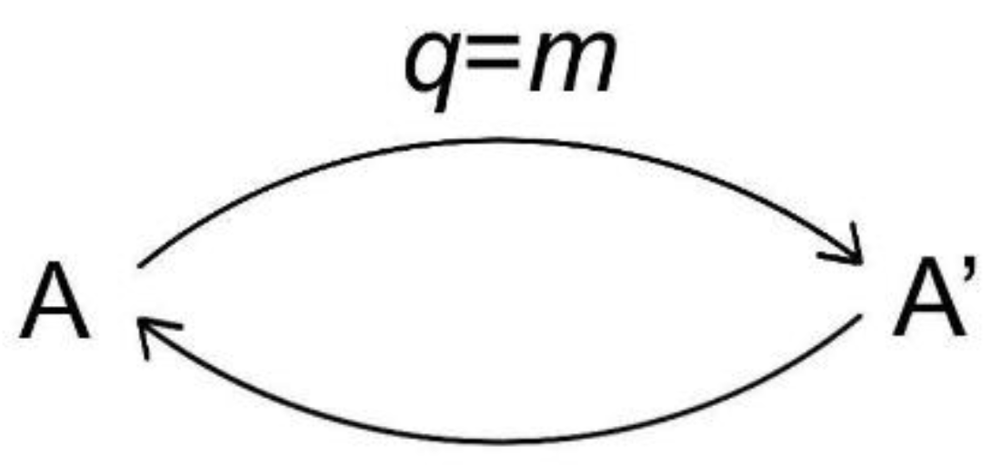
Postulate 3.1 (coupling constant). The Boolean rotation couples two Boolean poles, and . It generates the coupling constant, called metalogic charge, denoted as q, which is also called the rotational mass, denoted as m. This is roughly showed below.
Figure 3.
1.
In physics, a massive spin half spinor field has no clear helicity and it allows for superposition states, such as the Dirac spinor introduced earlier. Our argument here is more general.
Theorem 3.1 (superpositions). Boolean spinor with polarization poles (, will produce superpositions under the Boolean rotation (2.1).
Proof. Consider the complexification (2.4), we have the base states . The superpositions are any linear combination of and : , where and are complex numbers.
Theorem 3.2 The Riemann sphere of two-state system is a twistor.
Proof. The antipodal of a Riemann sphere (, is a Boolean Weyl-spinor, denoted as. By Postulate 2.2 and Theorem 3.1, the superpositions states of the Riemann sphere is characterized as the Dirac spinor, denoted as . To compose the two spinors, it satisfies the twistor equation (2.7), .
4. Geometry of Wavefunctions
4.1. Wavefunction as a dual-process
Wavefunction is the heart of the quantum mechanics (Dirac, 1930/1958). Von Newman (1932) regards that the wavefunction in quantum mechanics involves two processes. One is the U-process (unitary) and the other is the R-process (reduction). During the U-process, the wavefunction evolves by following the Schrödinger equation:
In this equation, the imaginative i makes the U-process not directly observable. The equation contains the mass term m such that the U-process produces superposition states. Superpositions occur when the particle is massive and spins half, which is the intrinsic property of a quantum particle with the internal space.
The R-process is based on observations. Quantum observations involves the so-call Yes/No measurement (von Newman, 1932; Penrose, 2004). There is a long-standing controversy about the measurement problem, which Penrose also calls the measurement paradox. It is still an open conjecture. The Yes/No measurement can be seen as the polarization of the wavefunction.
Penrose denotes Schrödinger evolution by U and state reduction by R. He wrote, “This alternation between the two completely different-looking procedures would appear to be a distinctly odd type of way for a universe to behave!” The figure Penrose provided is roughly given below.
Penrose wrote further, “Why is R mathematically inconsistent with U? Perhaps the most obvious reason is that R represents a discontinuous change in the state vector, whereas U always acts continuously. But even if we imagine that the ‘jump’ induced by R is not absolutely instantaneous, there would be trouble with uncertainty because of the lack of determinism in R. Different alternative outcomes can result from the same input, which is something that never happens with U. Moreover, a theory that makes R into a real process cannot ever be unitary when a (non-trivial) quantum jump – in accordance with R – actually takes place.”
In this section, we provide an alternative view for such a dual-process of the wavefunction.
4.2. The R-process and the Yes/No measurement
“Once animals begin to approach certain things and avoid others, the ability to adjust their judgement of good and bad becomes a matter of life and death. … “Learning was not the core function of the first brain; it was merely a feature, a trick to optimize steering decisions. Association, prediction, and learning merged for tweaking goodness and badness of things.” (Max Bennet, A brief History of Intelligence. 2024). The Good/Bad distinction is the origin of the Yes/No measurement.
Von Neumann pointed out (1932, 1955/2018) that experimental observations in quantum mechanics can be reduced to a kind of "Yes/No" measurement. Penrose also elaborates on this idea in details. In short, in a quantum experimentation, the particle detector is referred to as the "Yes gate." When the particle source excites a particle and the detector receives it, it is said that the particle has entered the Yes gate. If the detector does not receive the particle, rather than saying the particle was not excited, it is said that the excited particle has entered the "No-gate." This description differs from classical mechanics and is counterintuitive, but it is a key feature of quantum mechanics.
Such "Yes/No" type observations are mathematically represented by the Dirac δ-function (Griffel, 2002):
This function consists of two formulas. The first formula states that if an excited particle enters the Yes gate (the detector, the correct answer, or the predicted future event), the function value is infinite; if the excited particle enters the No gate (not detected, the question is answered incorrectly, or the prediction is wrong), the function value is zero. The second formula is the indefinite integral of the first formula, and its value equals a constant. Here, the second formula tells us that regardless of whether the particle enters the Yes gate or the No gate, the particle has been excited. In philosophical terms, the first formula of the Dirac function can be considered its epistemological support, while the second formula represents its ontological commitment. The Dirac function almost perfectly characterizes "Yes/No" type observations, but it is not a mathematically well-defined function.
It was not until later that the measurement theory in mathematics was developed. In this theory, starting from the second formula of the original Dirac function (the integral formula) to make an ontological commitment, and using the first formula as the integrand, (the test function) to provide the epistemological path, requires that this test function must have at least one "support point." This support point is the excited particle detected by the original quantum observation detector.
4.3. Projections as polarizations
Let us review a few key concepts concerning the measurement paradox.
The first key concept is the Observable Q. The measurement paradox can be simply characterized as U-procedure versus R-procedure. Here U stands for unitary, and R stands for reduction. On one hand, the U procedures work so supremely well for simple enough systems, whereas on the other, we have to give up on U and abruptly, yet stealthily, interpose the R process from time to time. The two quantum processes, U and R, are in conflict. On the one hand, U-procedure is the deterministic process of unitary evolution which can be described by Schrödinger’s Equation which controls the clear-cut temporal evolution of a definite mathematical quantity, namely the state vector The wavefunction in the U process is single-valued, continuous, differentiable, and square-integrable.R-Procedure is the quantum state reduction which takes place when a ‘measurement’ is performed. The R process is a discontinuous random jumping of this same , where only the probabilities of the different outcomes are determined.
The observable operator Q is responsible to transfer from U-process to R-process. Q has two eigenstates, say, one is YES and the other is NO. How the Q operator works is a mystery. Penrose (2004) reviewed and discussed six approaches toward this problem. An interested reader may read his book, particularly its §29.
The second key concept is the Projector E. The projector E was originally introduced by von Neuman (1955). Penrose (2004) provides a thorough characterization of E. Indeed, his §22.5 is titled: Yes/No measurement. It is the view of von Neuman and Penrose that all the quantum measurements are the Yes/No type measurements. Once Q turns a quantum process into the R-procedure, then E projects the quantum state to Yes or else No. In other words, the projector E has exactly two eigenstates.
The third key concept is the Yes/No measurement. The Yes/No type measurement originally proposed by von Neuman (1955) and outlined in detail by Penrose (2004). Both authors stated that all the quantum theoretic experiments are Yes/No type measurements, characterized by the projector E. Examples of experiments in physics, e.g., the Stern-Gerlach experiment, can be found in Sakurai.
E-projector is defined as follows. Consider an any given wavefunction , ranges over all space points of X. For any given space point Q where stands for a testing point. Then, E projects to be Yes or No. We call it the E operation, which stands for the any given the Yes/No observations. In measurement theory (, in (4.2) is called a testing function, and in (4.1) is called the supporting point of . Now we look at an important property of the -function.
Let be an any given one-dimensional wavefunction. Assume () is a R-interval. Then we have
(4.3)
It is held simply by the well-known selectivity of the Dirac -function.
To solve the measurement paradox, the existentiality is not enough. It needs to further formulate a constructive proof. The Yes/No type measurement enables us to recapture paradox of U-process vs. R-process. From mathematical perspectives, it is a single-valued vs. two-valued problem. During the U-process, the wavefunction is single valued. While during the R-process, any measurement of the wavefunction becomes two-valued. However, the two processes must share the same semantics, namely the squared modulus, i.e., the Born probability. Thus, how to generate the required Born probability from R-process is a sensitive issue.
We can see from the above discussion that the projection operator polarizes the wavefunction to two poles: Yes or No. There are two issues for the measurement problem. The first is the semantic one. The wavefunction semantics is the amplitude semantic. The meaning of the U-process of a wavefunction is its amplitude, which is the Born probability that is single-valued. While the R-process is two-valued process, resulting in Yes/No measurement. The second issue is syntactic. The U-process is characterized by the Schrödinger equation, in which the wavefunction is a continuous function, while the R-process is discrete. We solve the first issue in the next section and the second issue in the following section.
4.4. Stochastic sampling
Yang (2024) proposed a stochastic sampling method to generate Born Probability from the R-process. Let us consider an any given wavefunction (x), where x ranges over all of the space points. We assume that (x) is one-dimensional without loss of generality for multi-dimensions. Thus, the corresponding Hilbert space we are currently discussing is one-dimensional, denoted by H. Hence, we may treat all the vectors in H as space points also without loss of generality. Now, it introduces an observation operator Q, which is defined below.
Definition 4.1 For any given a, , . We call that is the observational conjugate of . Accordingly, we define | ranges over all possible observational . Call the observational dual space of .
The necessity of the distinction between the space points and the observational points is analytical to the distinction between of the intuitive natural numbers and the set-theoretic enumerers in Gödel’s work (Yang, 2022).
Consider the power set of , . Now, we start to select the elements from . Notice that this selection process is countable, but the cardinal number of is an uncountable infinity. We may reasonably assume this selection process is stochastic.
Definition 4.2 We introduce a new variable , . Of course, we also have , so we can introduce another variable , where the superscript j indicates the jth element stochastically selected from , the subscript i indicates that x ranges over only those space points within . It is easy to see that connects and . Accordingly, we have
Definition 4.3 We introduce a new operator , called the sample generator. , . Call the testing adjoint of .
Definition 4.4 Stochastic sampling: 1. For any given once a is stochastically selected, its adjoint becomes a testing sample. 2. For any , if it has not been selected, then its adjoint is not a testable sample yet.
Note, this definition is analytical to the expressibility in Gödel’s work [6]. (Hint, the notion of expressibility is necessary to bridge the relations in Piano arithmetic and functions in the first order theory.) While here the definition of stochastic sampling process is necessary to bridge any from sampling perspectives.
Definition 4.5 (R-process). Let stand for an any given sample , denote a YES/No type experiment, and q be a Yes/No type stimuli that can use to test . By Dirac bra-ket formalism, we can write this structure as . When gives the stimulus q to , each operational conjugate in returns a Yes/No type response. Thus, is a function of . This is called the R-procedure of the wavefunction. Note, this idea is from Feynman (1965), who calls the final state and the initial state of a quantum theoretic experiment.
Definition 4.6 (Sample space). The sample space for the Yes/No type measurement is two-valued, i.e., This means the E-projector has two and only two eigenstates, of which the eigenvalues are Yes and No.
Definition 4.7 (Sample phase). Consider projector E, for each proper sample of Yes/No type measurement, produces a pair of the yes-number c and the no-number d, which in turn produces a sample phase with respect to the exponential form of . All the possible sample phases form an group, write it G. From Definitions 1 to 4, it is easy to see that G is originally generated from the wavefunction , so we write G as .
Because symmetry, the stochastic sampling here satisfies the required conservativeness. It is worth mentioning that, in addition to the well-documented dynamic phase and Berry phase in the literature of dynamic analysis, the sample phase introduced here is the third kind of phase. This is one significant character of the R-procedure. For the U-procedure, we have the dynamic phase potential group, write it as .
Definition 4.8 (Linearization). The linearization operator L is defined by ).
Definition 4.9 (Sample Born probability). For any given testing sample , which produces a yes-number and a no-number . The sample Born probability is defined by
. (4.4)
Born probability is a kind of explanation, which serves as a semantics for the evolution of wavefunction. As Penrose pointes out [1], the U-procedure and R-procedure must share the same semantics, i.e., the squared magnitude of two eigenvalues.
Theorem 4.1 (Born rule). The Born probability defined by Definition 9 obeys Born rule.
Proof. Let be a testing sample. eigenstates, Yes or else No. Assume the eigenvalue for Yes is c and the eigenvalue for No is d. Then, by Definition 8, we have ). Hence, by Definition 9, we have
( . (4.5)
This shows that Definition 8 is conformal with respect to the Born rule.
4.5. Geometry of the wavefunction
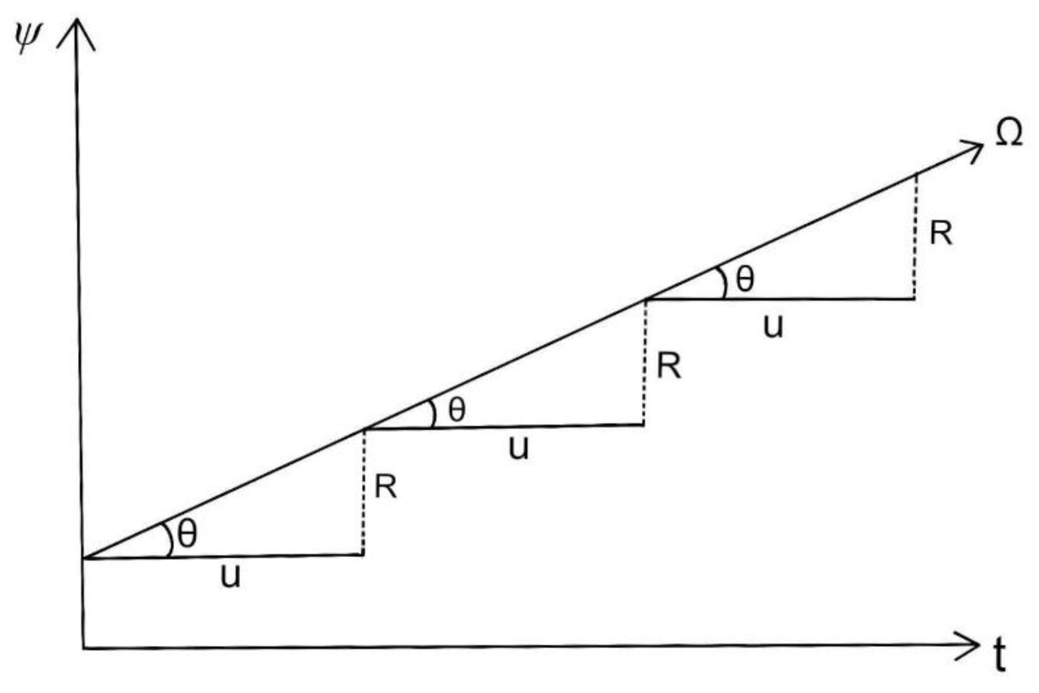
Consider the Yes/No measurement (Yes, No) as a Boolean Weyl-spinor . By Theorem 2.1, rotates through complexification. The phase of such a rotation is a continuous variable. Call this spinor the R-spinor. As we analyzed earlier in §2 and §3, The decomposition and reassemble of this R-spinor result in a Boolean Dirac-spinor with superpositions. Call this new spinor the U-spinor. Denote the R-spinor as and the U-spinor as . To compose the two spinors, it satisfies the twistor equation (2.7), . Recall the Figure 4.1, we now have a new geometry of the wavefunction as follows.
In this new picture, the wavefunction is represented as a twistor , which connects straight paths. It is not hard to characterize the twistor path by the path integral. In addition, the angle in Figure 4.2 is actually the dynamic phase from gauge field theoretic perspectives; thus, it would be interesting to address the gauge symmetry issue. These are topics that go beyond the scope of this paper.
5. Concluding Remarks
Remark 1. As Penrose (2004) argued convincingly, the complex field has many miraculous properties. The Boolean rotation through complexification introduced in this paper is a fantastic example. This looks like a small and simple change, but is actually a big move in analytic sciences including logic, mathematics, and computer science.
Remark 2. Logic and the Boolean algebra are embodied in mathematical language. Mathematics needs to take polarization as well as superposition states into account. If the logic does not rotate, it can only cover the polarizations but not superpositions. Consequently, in other words, the logic foundation of mathematics can only be limited and partial. The Boolean rotation theorem changes the situation. It opens the possibilities to account for superposition states as well. This would allow us to build the more complete logical foundation of the mathematics.
Remark 3. Riemann sphere of two-state systems and wavefunction in quantum mechanics are two sample mathematical domains to demonstrate the claims in Remark 2.
Remark 4. Since Gödel’s independence result (1931), the so-called Hilbert second conjecture has been seemingly hopeless. But careful analysis would disclose that the self-referential statements are superposition states. Indeed, the self-referential statements involve two Gödel numbers and can be characterized by the complex numbers and spinor fields. This is an interesting topic for further research.
Remark 5. The Boolean rotation allows we characterized both polarization states and superposition states as spinors, and together they satisfy the twistor equation. This geometric method is general and has a wide range of implications. One significant implication is of the digital language, which is the foundation of computer science and artificial intelligence. It is not hard to treat the bits as polarized Boolean Weyl-spinors without superpositions (Wheeler, 1989) and the qubits as the Boolean Dirac-spinors with superpositions. This will be our immediate next issue to address.
Acknowledgments
The author thanks Yong-Shi Wu for helpful and inspiring discussions.
References
- Bell, J.; Machover, M. A course in Mathematical Logic; North Holland Publisher, 1977. [Google Scholar]
- Dirac, P. A. M. Principles of Quantum Mechanics; Oxford University Press, Pearson Education, Inc.: New York, 1930/1958. [Google Scholar]
- Griffel, D. H. Applied Functional Analysis; Dover Publications, Inc.: Mineola, New York, 1981/2002. [Google Scholar]
- Penrose, R. The Road to Reality: A Complete Guide to the Laws of Universe; Random House Inc.: New York, 2004. [Google Scholar]
- von Neuman, J. The Mathematical Foundations of Quantum Mechanics; Princeton University Press: Princeton, New Jersey, 1955/1983. [Google Scholar]
- Wheeler, J. A. INFORMATION, PHYSICS, QUANTUM: THE SEARCH FOR LINKS. Reproduced from Proc. 3rd Int. Symp. Foundations of Quantum Mechanics, Tokyo, 1989; pp. 354–368. [Google Scholar]
- Yang, Y. The Revised Schrödinger Equation as a Solution of Measurement Paradox: A Unified Model of the U-procedure and R-procedure. 2024. [Google Scholar] [CrossRef]
- Zee, A. Quantum field Theory in a Nutshell; Princeton University Press, 2010. [Google Scholar]
Figure 2.
Riemann sphere of two-state system.
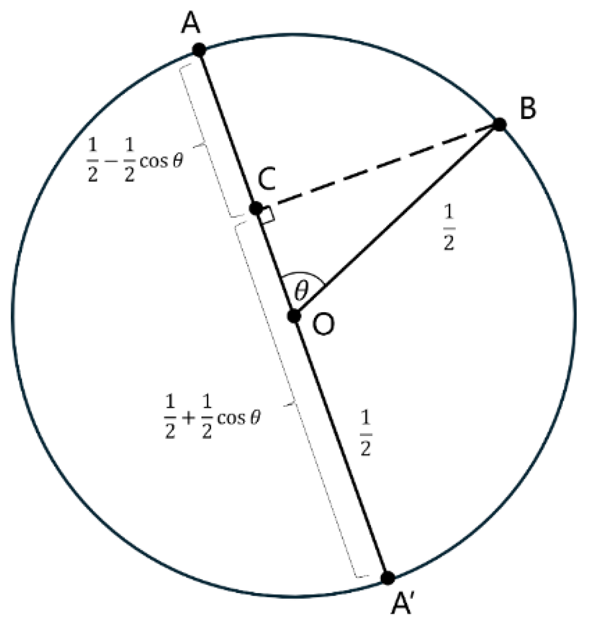
Figure 4.
1.
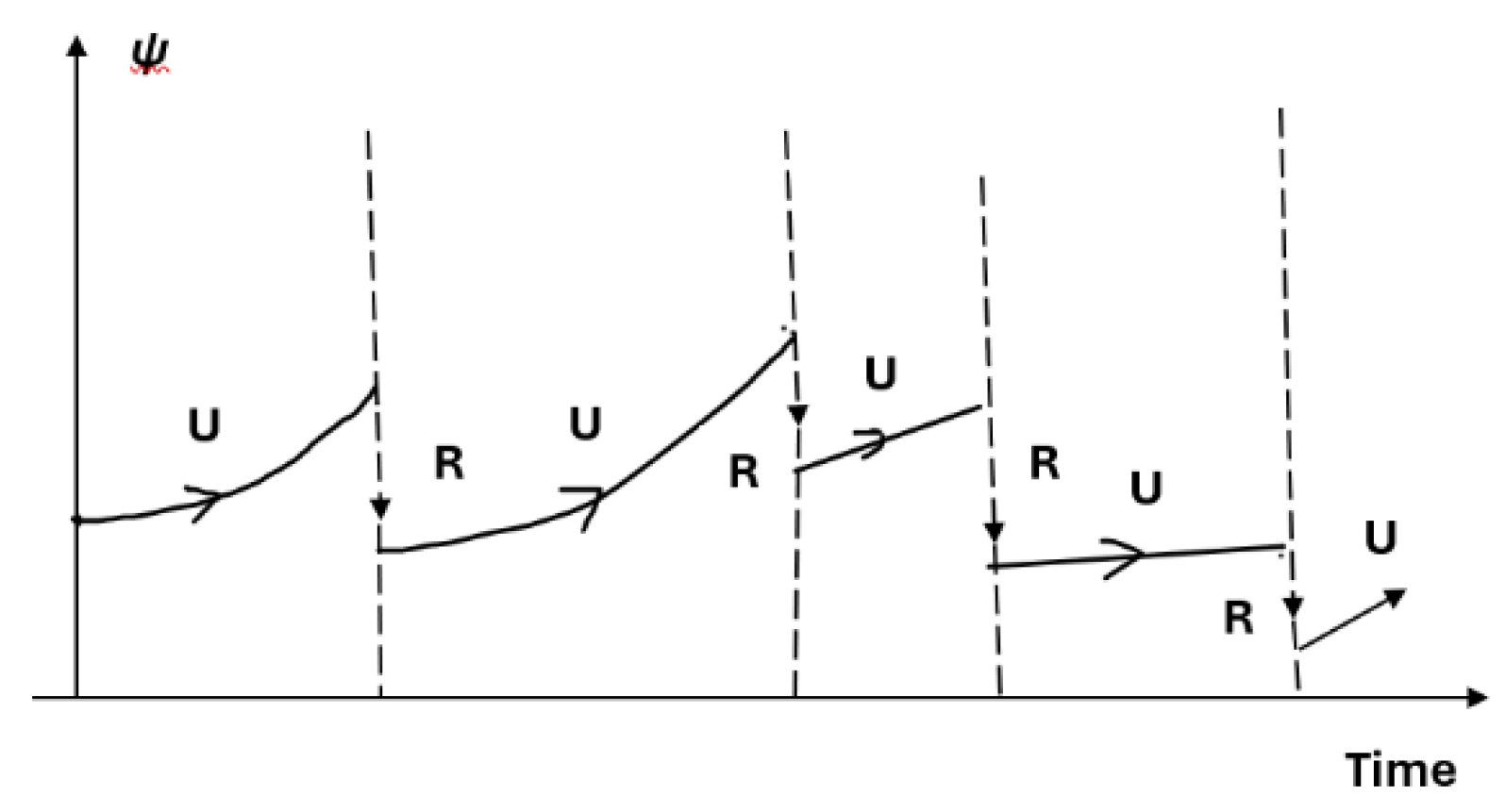
Figure 4.
2.
Disclaimer/Publisher’s Note: The statements, opinions and data contained in all publications are solely those of the individual author(s) and contributor(s) and not of MDPI and/or the editor(s). MDPI and/or the editor(s) disclaim responsibility for any injury to people or property resulting from any ideas, methods, instructions or products referred to in the content. |
© 2026 by the authors. Licensee MDPI, Basel, Switzerland. This article is an open access article distributed under the terms and conditions of the Creative Commons Attribution (CC BY) license (http://creativecommons.org/licenses/by/4.0/).
Copyright: This open access article is published under a Creative Commons CC BY 4.0 license, which permit the free download, distribution, and reuse, provided that the author and preprint are cited in any reuse.


