Submitted:
30 January 2026
Posted:
30 January 2026
You are already at the latest version
Abstract
In this paper, we present a deep neural network–based approach for computing radar cross section (RCS) over a wide frequency band and a broad range of incident angles.The proposed network, termed WBRCS-Net, is designed to converge to the solution of the method of moments (MoM) formulation by minimizing a mean-squared residual loss without explicitly solving the MoM linear system, thereby avoiding the numerical instabilities commonly encountered in conventional iterative solvers.
Moreover, by using only the frequency and incident angle as inputs, WBRCS-Net enables wideband RCS prediction over a broad range of incident angles while substantially simplifying the network architecture. The performance of WBRCS-Net is evaluated on perfectly electrically conducting (PEC) spheres and cubes and compared with the Maehly approximation based on Chebyshev polynomials. Experimental results show that, once trained, WBRCS-Net provides accurate and stable wideband RCS computations over a wide range of incident angles with instantaneous inference speed, highlighting a key advantage of the neural network–based approach.
Keywords:
radar cross section (RCS)
; method of moments (MoM)
; wideband
; wide incident angle
; neural network approach
1. Introduction
The radar cross section (RCS) is a fundamental metric for radar detection and target identification, and it is a critical design driver for stealth applications. RCS can be computed from the scattered electromagnetic fields obtained by solving electromagnetic scattering problems. Owing to its high accuracy and broad applicability to arbitrarily complex three-dimensional geometries, the method of moments (MoM) is widely used to compute scattering fields [1]. MoM is a numerical technique based on surface discretization, in which continuous electromagnetic integral equations are transformed into a finite-dimensional linear system characterized by an impedance matrix and an excitation vector, from which the surface current vector is obtained. However, achieving higher accuracy requires finer surface discretization, which significantly increases the dimension of the impedance matrix.
Consequently, building and solving large linear systems is a major bottleneck in MoM-based RCS computation [2]. Conventional iterative solvers, such as the Conjugate Gradient (CG) and Biconjugate Gradient (BiCG) methods, have been widely adopted to accelerate the solution process [3,4]. Nevertheless, for high-frequency scenarios and electrically large or geometrically complex targets, the impedance matrix becomes extremely large, leading to high computational complexity and slow or unstable convergence.
The computational burden is further exacerbated in wideband RCS analysis, where RCS must be evaluated over a broad frequency range. In such cases, the impedance matrix must be built and the corresponding linear system solved at each frequency point [2]. To alleviate this cost, various interpolation techniques have been developed to approximate impedance matrices at intermediate frequencies. Quadratic interpolation was introduced in [5], and cubic polynomial interpolation was later shown to improve accuracy [6].
To further reduce the cost associated with repeatedly solving linear systems, several methods have been proposed to approximate the MoM solution vector over frequency. The asymptotic waveform evaluation (AWE) relies on high-order frequency derivatives of the impedance matrix to approximate the MoM solution vector, and the need to compute and store these derivatives can impose significant memory overhead [7]. To address this limitation, Chebyshev polynomial approximation methods have been introduced, which reconstruct the MoM solution vector using samples at Chebyshev nodes [8,9]. Building on this idea, Maehly approximation, a rational-function method based on Chebyshev polynomials, has been proposed to further improve approximation accuracy [10] and has since been widely applied in wideband RCS computation [11,12,13,14].
In addition to frequency dependence, RCS also varies with the incident angle. Consequently, wideband and wide incident angle RCS analysis requires repeated MoM solutions over a two-dimensional frequency–angle domain. Each frequency–angle pair corresponds to a distinct MoM linear system, rendering direct computation prohibitively expensive. To reduce this cost, Maehly approximation has been extended to a two-dimensional frequency–angle formulation for efficient wideband and wide incident angle RCS computation [15]. Nevertheless, these interpolation methods necessitate solving large MoM linear systems at every sampled frequency–angle point, leaving the fundamental challenge of large-scale linear system solves unresolved.
Recently, neural networks have been explored for solving large-scale linear systems due to their modeling flexibility and computational efficiency [16,17,18]. In [19], a neural network directly maps discretized geometric grid points to the MoM solution vector by minimizing the residual of the corresponding MoM linear system. While promising, this approach requires a high-capacity network to represent the extremely high-dimensional input–output mapping and does not inherently support interpolation with respect to frequency or incident angle, thereby limiting its applicability to wideband RCS analysis and scenarios involving a broad range of incident angles.
In this paper, we propose WBRCS-Net, an efficient neural-network-based framework for solving large-scale linear systems arising from the method of moments (MoM), specifically tailored for wideband and wide–incident-angle RCS computation. Unlike existing neural-network-based approaches that learn high-dimensional–to–high-dimensional mappings, WBRCS-Net predicts the MoM solution vector conditioned solely on the frequency and incident angle by learning a low-dimensional–to–high-dimensional mapping, which substantially simplifies the network architecture. Specifically, the network takes two scalar inputs—the frequency and the incident angle—and outputs the corresponding MoM solution vector. This formulation provides intrinsic interpolation capability across both frequency and incident angle, enabling accurate prediction at intermediate frequency–angle points without additional MoM solves.
The training time of WBRCS-Net depends on the size of the MoM system and the number of training points, and may be relatively long. However, once trained, WBRCS-Net computes RCS over a wide range of incident angles with instantaneous inference speed, highlighting a key advantage of the neural network–based approach.
To evaluate WBRCS-Net, we conduct monostatic RCS experiments on two perfectly electrically conducting (PEC) targets: a sphere and a cube. We first demonstrate the convergence behavior of WBRCS-Net at several representative frequencies. Using these sampled points as training data, we evaluate the prediction performance of WBRCS-Net over wideband frequencies, in comparison with the widely used Maehly approximation. The two-dimensional interpolation capability of WBRCS-Net across frequency and incident angle is illustrated by visualizing the resulting 3D RCS surface. We further compare the MoM reference solutions and the WBRCS-Net predictions through cross-sectional slices along fixed-frequency and fixed-angle cuts.
2. Related Works
2.1. Method of Moments for Surface Current
The method of moments (MoM) [1] is a widely used numerical method for computing the induced surface current on a triangulated surface approximating the target object in electromagnetic scattering problems. The unknown surface current is represented as a linear combination of given surface basis functions, (e.g., Rao-Wilton-Glisson (RWG) functions defined on triangular meshes with L edges [20]),
MoM converts the continuous EFIE into a discretized linear system for the surface current coefficient vector (referred to as the MoM solution vector, or simply the solution vector) at the incident-field frequency f and incident angle ,
where is the impedance matrix and is the excitation vector given by [21]
where is the Green’s function, and is the incident electric field at frequency f and incident angle .
2.2. Maehly Approximation
The RCS at a frequency f is computed using the surface current coefficient vector that is obtained from the MoM linear system (2) with respect to f. To compute the RCS over a broad frequency band, the MoM linear system must be built and solved at many frequency points, which is computationally expensive. Maehly approximation [22] is the most popular method to alleviate this burden. The Maehly method accurately interpolates the surface current coefficient vector at a given frequency using a rational function of Chebyshev polynomials [23] obtained from the Chebyshev-Gaussian sampling frequencies [14].
For the given frequency range , the Chebyshev-Gauss sampling nodes for sample points are given as
The Maehly method approximates the coefficient vector with a rational function of Chebyshev polynomials
where is the normalized frequency of , i.e. , is a Chebyshev polynomial of degree i[23], and are Maehly coefficients that can be recursively computed [14].
Since the RCS computation depends on both frequency and incident angle, the surface current coefficient vector can be treated as a bivariate function . Following the two-dimensional approximation approach in [15], each surface current coefficient is approximated over the frequency and angular domains with a rational function of bivariate Chebyshev polynomials constructed on Chebyshev-Gauss sampling nodes:
where is the normalized incident angle of , i.e., , with denoting the number of sampled incident angles, and the Maehly coefficients can be recursively computed [15].
3. Methods
3.1. Architecture of WBRCS-Net
Figure 1 illustrates the WBRCS-Net, which solves the MoM linear system using a neural network approach. We design the WBRCS-Net to output a solution vector . Since the solution vector is complex-valued, the number of output nodes is set to twice the dimension of the solution vector. Odd-numbered output nodes represent the real part of the solution vector, while even-numbered output nodes represent the imaginary part. We construct the WBRCS-Net using only two residual blocks and fully connected (FC) layers. It has two input nodes that receive the frequency and incident angle. The number of nodes in the hidden layers is expanded step-wise from 2, , L, and , where L is the number of edges in the triangulated object. Hence, the proposed WBRCS-Net has total parameters. The activation function used is the hyperbolic tangent function.
3.2. WBRCS-Net for MoM Solutions
In this section, we present a neural-network-based approach for solving Method of Moments (MoM) systems using WBRCS-Net. For a given frequency f and incident angle , we construct the impedance matrix and the excitation vector . The solution of the resulting linear system is obtained by minimizing the following residual loss via back-propagation:
where denotes the output of WBRCS-Net at the t-th iteration, and L is the dimension of the MoM linear system.
Since the impedance matrix and the excitation vector remain fixed throughout all iterations, the network input does not encode any physical parameters and can be set to arbitrary dummy values. Instead, WBRCS-Net learns an iterative update rule that progressively reduces the residual of the MoM linear system. In this sense, WBRCS-Net can be interpreted as a learned iterative solver whose update dynamics are optimized through training.
3.3. Training WBRCS-Net for Wideband Frequency and Wide Range Incident Angle
To extend WBRCS-Net to wideband frequencies and a wide range of incident angles, we construct impedance matrices and excitation vectors over a set of training points and , where and denote the numbers of training frequencies and incident angles, respectively.
Accordingly, the residual loss in (8) is extended to all training frequency–angle pairs as
With this formulation, the output of WBRCS-Net, , explicitly depends on the frequency and incident angle, enabling the network to learn a continuous mapping from to the MoM solution vector.
In order to accelerate training speed, the first step of back-propagation is performed directly using the following pre-computed gradient of the loss function, instead of using the automatic optimizer:
where is the conjugate transpose of . To avoid computing and for each update, we pre-compute
This pre-computation method enables neural network training much faster than the conventional optimizer method.
The training time of WBRCS-Net depends on the number of edges (L) and the number of training points, and is on the order of minutes in our experiments. In contrast, the prediction (inference) runtime for an arbitrary test point, specified by frequency and incident angle, is only seconds to compute the solution vector, highlighting a key advantage of the neural network–based approach.
3.4. RCS Computation
The RCS computation diagram is shown in Figure 2. Using the trained WBRCS-Net, the surface current is obtained from (1). Then, the RCS is computed using the surface current [21]. The formula is as follows:
where is a given frequency, is the speed of light in vacuum, is the wavenumber and is the unit observation vector.
4. Experiment Settings
4.1. MoM Configuration
In order to train WBRCS-Net, impedance matrices and excitation vectors were built at the training sample frequencies using the python-based BEM++ package [24]. The surface currents were expanded with Rao–Wilton–Glisson (RWG) basis functions [20] on triangular surface meshes for perfectly electrically conducting (PEC) objects. The incident wave is a plane wave polarized along the x-axis, and its propagation direction is defined by . In the frequency-only setting, the incident angle is set to zero, i.e., (propagation along the +z-axis), while in the joint frequency–angle setting, ranges from to . The RCS is evaluated in a monostatic configuration, where the observation direction is opposite to the propagation direction of the incident wave.
We evaluated two PEC objects: a sphere and a cube. For the sphere, two radii were considered (3cm and 4cm), and for the cube, two side lengths were considered (3cm and 6cm), resulting in four experimental cases in total. The corresponding surface meshes are illustrated in Figure 3. The numbers of edges for the four cases are 1641 (sphere, 3cm), 1884 (sphere, 4cm), 810 (cube, 3cm), and 1788 (cube, 6cm). All cases are evaluated over the frequency range from 2 GHz to 12 GHz.
4.2. Data and Training Setting
For the sphere and cube, we consider several different numbers of training frequency samples. We set the number of training epochs separately for each training frequency-sample setting, increasing the number of epochs for larger training frequency sets. The training frequencies are uniformly sampled over the given frequency band. All frequencies are converted to GHz and used as inputs to the neural network. All incident angles are normalized from the range of to to the range of 0 to 1 and used as inputs to the neural network. Training is performed in a full-batch setting, where all training samples are processed simultaneously in each optimization step using the Adam optimizer with a learning rate of 0.001. All experiments are carried out on an NVIDIA H100 GPU.
5. Experiment Results
5.1. Demonstration of WBRCS-Net for MoM
We conducted experiments to demonstrate the feasibility of the proposed WBRCS-Net for MoM. The experiment was conducted on a unit sphere, triangulated with , at a frequency of 100 MHz with the incident angle fixed at . During training, the network input was set to a constant dummy value of 1 for the frequency and 0 for the incident angle.
Figure 4 presents the training loss over epochs, demonstrating stable and consistent convergence. Figure 5(a,b) visualize the real component of the surface currents obtained from the MoM solution and the WBRCS-Net, respectively. The surface currents predicted by WBRCS-Net closely match the MoM surface currents. The corresponding RCS values computed from the MoM and WBRCS-Net surface currents are 4.15204 and 4.150207, respectively, indicating near-identical RCS results. After 5,000 iterations, WBRCS-Net achieves a residual error of approximately with a runtime of 5.35 seconds on an NVIDIA H100 GPU.
5.2. Wideband RCS Computation on the Sphere
In Figure 6, we compare the wideband RCS obtained using the Maehly approximation and WBRCS-Net under different numbers of sampled frequencies. Figure 6(a,b) present the results for a sphere with a radius of 3cm () when the number of sampled frequencies is and , respectively. The black, blue, and red curves correspond to the RCS computed by MoM, Maehly, and WBRCS-Net, respectively. For WBRCS-Net, the training runtime is 334.1 seconds for (120,000 epochs) and 579.8 seconds for (200,000 epochs), while the inference time is only seconds per test point. For the 3cm sphere, both methods exhibit good interpolation performance.
Figure 7 presents an experiment designed to evaluate interpolation performance under a more rapidly changing RCS response. We increase the sphere radius to 4cm (), which yields an RCS curve with more rapid changes. We consider two training frequency-sample settings, and ; for WBRCS-Net, the training runtime is 352.9 seconds for (120,000 epochs) and 609.1 seconds for (200,000 epochs), while the inference time is only seconds per test point. When the RCS varies more rapidly, the Maehly approximation exhibits unsatisfactory interpolation performance even as the number of sampled frequencies increases from to . In contrast, WBRCS-Net maintains reliable interpolation performance even with , and with , the computed wideband RCS closely matches the MoM reference. WBRCS-Net produces a smooth and well-behaved wideband response without abrupt spikes, indicating improved robustness under rapidly varying RCS behavior compared with the Maehly approximation.
To provide a quantitative comparison, Figure 8 reports the mean squared error (MSE) with respect to the RCS directly computed by MoM, evaluated at the at test frequencies in every 100 MHz. Figure 8(a) summarizes the results for the 3cm sphere by sweeping the number of training frequencies from 9 to 30. In this less rapidly changing case, the MSE gap between the Maehly approximation and WBRCS-Net remains relatively small, indicating comparable interpolation performance. However, as shown in Figure 8(b), for the more rapidly changing 4cm sphere, WBRCS-Net achieves lower MSE than the Maehly approximation for almost all sampling configurations. Overall, these results suggest that WBRCS-Net provides more accurate and reliable wideband interpolation when the RCS exhibits more rapid changes with frequency.
5.3. Wideband RCS Computation on the Cube
In Figure 9, we compare the wideband RCS of the cube with an edge length of 3cm () computed using the Maehly approximation and WBRCS-Net. For WBRCS-Net, the training runtime is 286.2 seconds for (120,000 epochs) and 488.1 seconds for (200,000 epochs), while the inference time is only seconds per test point. The RCS curve is relatively smooth across the frequency band, showing a single broad change followed by a gradual increase toward higher frequencies. When , the Maehly approximation shows a small spike around 12 GHz. When is increased to 30, both Maehly and WBRCS-Net yield accurate and stable wideband interpolation, closely following the MoM reference.
In Figure 10, we evaluate a more challenging case by increasing the cube edge length to 6cm (). Compared with the 3cm cube, the wideband RCS curve exhibits more frequent changes across the frequency band. For WBRCS-Net, the training runtime is 349.3 seconds for (120,000 epochs) and 599.9 seconds for (200,000 epochs), while the inference time is only seconds per test point. In Figure 10(a) with , the Maehly approximation is consistent with the MoM reference over most of the band. Interestingly, when the number of training frequencies is increased to in Figure 10(b), the Maehly result exhibits a slightly local mismatch around 12 GHz. In contrast, WBRCS-Net remains stable and closely aligned with the MoM reference for both and , demonstrating accurate and robust wideband interpolation even for an RCS curve with more frequent variations.
To provide a quantitative comparison, Figure 11 reports the mean squared error (MSE) relative to the MoM reference, evaluated at test frequency in every 100 MHz. Figure 11(a) summarizes the results for the 3cm cube by varying the number of training frequencies from 9 to 30. The MSE difference between the Maehly approximation and WBRCS-Net remains small across this range, indicating comparable interpolation fidelity; in some cases, the Maehly approximation even slightly outperforms WBRCS-Net. Figure 11(b) shows that for the 6cm cube, whose RCS response varies more rapidly with frequency, WBRCS-Net exhibits comparable MSE at lower sampling counts, while delivering lower MSE as the number of sampled frequencies increases. Overall, these results indicate that WBRCS-Net provides more accurate and reliable wideband interpolation when the RCS curve exhibits more frequent variations across frequency.
5.4. Wideband RCS Computation with Incident Angle on the Cube
Following the experimental setup in [15] for joint interpolation over frequency and incident angle, we consider a PEC cube with an edge length of 0.5cm, triangulated with , over a frequency band of 10–50 GHz and an incident angle range of . We construct a training set using frequencies and incident angles, yielding total 441 training points. WBRCS-Net is trained for 500,000 epochs, with a total training runtime of approximately 52 minutes, while the inference runtime is seconds per test point. For evaluation, we test on a dense grid with a 100 MHz frequency spacing and a angular spacing, resulting in test points. Figure 12 illustrates the predicted frequency–angle RCS as a 3D surface (in dB), providing an overall view of the joint variation with respect to frequency and incident angle.
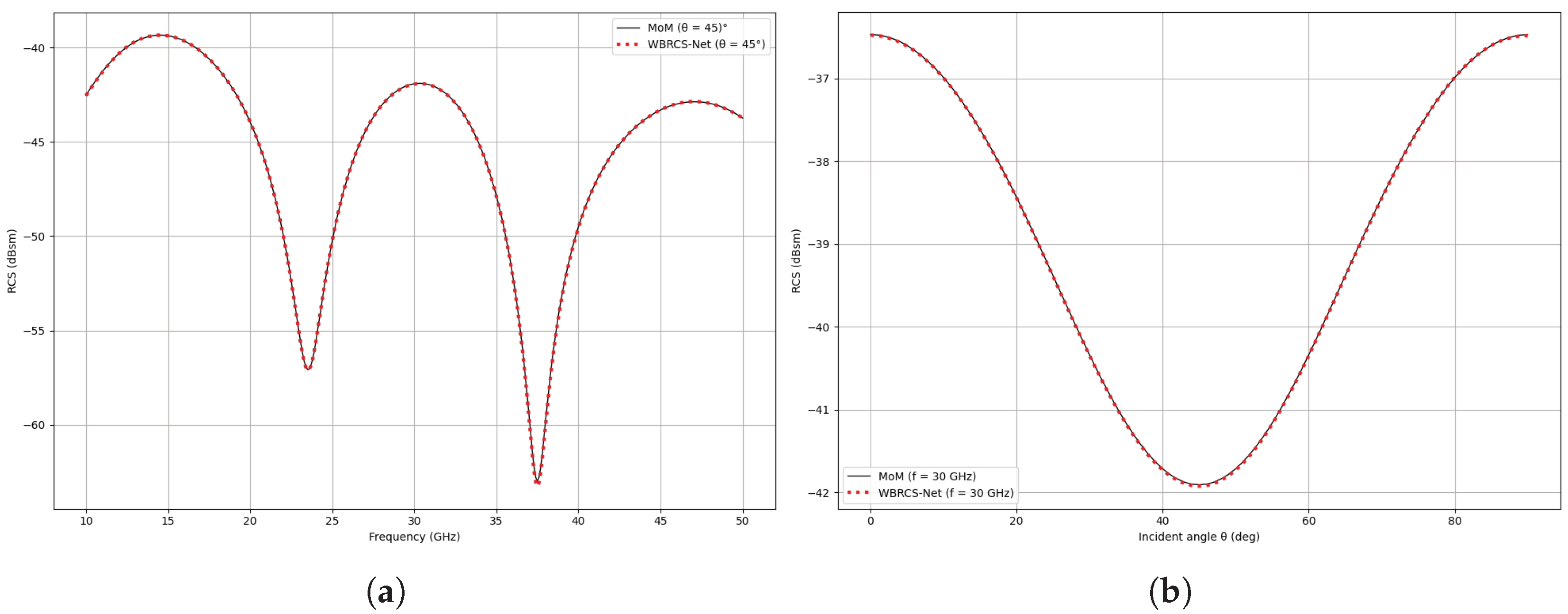
To validate the surface prediction against the MoM reference, we take representative one-dimensional cuts along each axis. Specifically, Figure 13(a) plots the RCS versus frequency at a fixed incident angle of , and Figure 13(b) plots the RCS versus incident angle at a fixed frequency of GHz. In both cuts, WBRCS-Net remains consistent with the MoM response, indicating accurate and stable interpolation in both frequency and angle. These results demonstrate that WBRCS-Net enables accurate and stable joint interpolation over frequency and incident angle.
6. Conclusions
In this work, we propose WBRCS-Net, an efficient neural network for solving large-scale linear systems arising in MoM-based RCS computation. By minimizing the residual error as a loss function, WBRCS-Net converges to the accurate solution of the underlying linear system. Moreover, by taking the frequency and incident angle as inputs, WBRCS-Net enables RCS interpolation at arbitrary frequency–angle points, thereby eliminating the need for repeated impedance matrix construction and corresponding linear solves. The effectiveness of WBRCS-Net is demonstrated on PEC spheres and cubes over a wide range of frequencies and incident angles, highlighting both its accuracy and interpolation capability.
References
- Gibson, W.C. The Method of Moments in Electromagnetics, 3rd ed.; Chapman and Hall/CRC: Boca Raton, FL, USA, 2021. [Google Scholar] [CrossRef]
- Liu, Z.-H.; Chua, E.K.; See, K.Y. Accurate and efficient evaluation of MoM matrix based on a generalized analytical approach. Prog. Electromagn. Res. 2009, 94, 367–382. [Google Scholar] [CrossRef]
- Sarkar, T.K.; Yang, X.; Arvas, E. A limited survey of various conjugate gradient methods for solving complex matrix equations arising in electromagnetic wave interactions. Wave Motion 1988, 10, 527–546. [Google Scholar] [CrossRef]
- Pocock, M.D.; Walker, S.P. The complex bi-conjugate gradient solver applied to large electromagnetic scattering problems, computational costs, and cost scalings. IEEE Trans. Antennas Propag. 1997, 45, 140–146. [Google Scholar] [CrossRef]
- Newman, E.H. Generation of wide-band data from the method of moments by interpolating the impedance matrix. IEEE Trans. Antennas Propag. 1988, 36, 1820–1824. [Google Scholar] [CrossRef]
- Li, W.; Zhou, H.; Hu, J.; Song, Z.; Hong, W. Accuracy improvement of cubic polynomial inter/extrapolation of MoM matrices by optimizing frequency samples. IEEE Antennas Wireless Propag. Lett. 2011, 10, 888–891. [Google Scholar] [CrossRef]
- Reddy, C.J.; Deshpande, M.D.; Cockrell, K.L.; Beck, G.A. Fast RCS computation over a frequency band using method of moments in conjunction with asymptotic waveform evaluation technique. IEEE Trans. Antennas Propag. 1998, 46, 1229–1233. [Google Scholar] [CrossRef]
- Chen, M.; Wu, X.; Huang, Z.; Sha, W.E.I. Chebyshev approximation for fast frequency-sweep analysis of electromagnetic scattering problem. Chin. J. Electron. 2006, 15, 736–738. Available online: http://hdl.handle.net/10722/148879.
- Chen, M.; Wu, X.; Sha, W.E.I.; Huang, Z. Fast frequency sweep scattering analysis for multiple PEC objects. Appl. Comput. Electromagn. Soc. J. 2007, 22, 250–253. Available online: https://aces-society.org/includes/downloadpaper.php?nf=4dbe68aa89b67796b7c1a2439d954fe5&of=J2007J10.
- Chen, M.; Wu, X.; Huang, Z.; Sha, W.E.I. Accurate computation of wide-band response of electromagnetic scattering problems via Maehly approximation. Microw. Opt. Technol. Lett. 2007, 49, 1144–1146. [Google Scholar] [CrossRef]
- Chen, M.; Wu, X.; Sha, W.E.I.; Huang, Z. Fast and accurate radar cross-section computation over a broad frequency band using the best uniform rational approximation. IET Microw. Antennas Propag. 2008, 2, 200–204. [Google Scholar] [CrossRef]
- Dong, H.-L.; Gong, S.-X.; Zhang, P.-F.; Ma, J.; Zhao, B. Fast and accurate analysis of broadband RCS using method of moments with loop-tree basis functions. IET Microw. Antennas Propag. 2015, 9, 775–780. [Google Scholar] [CrossRef]
- Wang, W.; Wang, H.; Li, Y.; Wang, X.; Fan, Z.; Gong, S. Efficient RCS computation over a broad frequency band using subdomain MoM and Chebyshev approximation technique. IEEE Access 2020, 8, 33522–33531. [Google Scholar] [CrossRef]
- Wang, X.; Gong, H.; Zhang, S.; Liu, Y.; Yang, R.; Liu, C. A hybrid method of adaptive cross approximation algorithm and Chebyshev approximation technique for fast broadband BCS prediction applicable to passive radar detection. Electronics 2023, 12, 295. [Google Scholar] [CrossRef]
- Ling, J.; Gong, S.-X.; Wang, X. A novel two-dimensional extrapolation technique for fast and accurate radar cross section computation. IEEE Antennas Wireless Propag. Lett. 2010, 9, 244–247. [Google Scholar] [CrossRef]
- Li, L.; Hu, J. An efficient second-order neural network model for computing the Moore–Penrose inverse of matrices. IET Signal Processing 2022, 16, 1106–1117. [Google Scholar] [CrossRef]
- Grementieri, L.; Galeone, P. Towards Neural Sparse Linear Solvers. arXiv 2022, arXiv:2203.06944. Available online: https://arxiv.org/abs/2203.06944. [CrossRef]
- Gu, Y.; Ng, M.K. Deep neural networks for solving large linear systems arising from high-dimensional problems. SIAM Journal on Scientific Computing 2023, 45(5), A2356–A2381. [Google Scholar] [CrossRef]
- Zhou, R.; Jiao, D. Efficient neural-network based solution of integral equations for electromagnetic analysis. In Proceedings of the 2024 IEEE International Symposium on Antennas and Propagation and INC/USNC-URSI Radio Science Meeting (AP-S/INC-USNC-URSI 2024), Florence, Italy, 14–19 July 2024; pp. 895–896. [Google Scholar] [CrossRef]
- Rao, S.M.; Wilton, D.R.; Glisson, A.W. Electromagnetic scattering by surfaces of arbitrary shape. IEEE Trans. Antennas Propag. 1982, 30, 409–418. [Google Scholar] [CrossRef]
- Sefi, S. Computational Electromagnetics: Software Development and High Frequency Modeling of Surface Currents on Perfect Conductors. Ph.D. Thesis, KTH Royal Institute of Technology, Stockholm, Sweden, 2005. Available online: http://urn.kb.se/resolve?urn=urn:nbn:se:kth:diva-590.
- Maehly, H.J. Rational approximations for transcendental functions. In Proceedings of the IFIP Congress 1959, Paris, France, 15–20 June 1959; pp. 57–61. Available online: https://unesdoc.unesco.org/ark:/48223/pf0000013303.
- Mason, J.C.; Handscomb, D.C. Chebyshev Polynomials; Chapman and Hall/CRC: Boca Raton, FL, USA, 2002. [Google Scholar] [CrossRef]
- Śmigaj, W.; Betcke, T.; Arridge, S.R.; Phillips, J.; Schweiger, M. Solving boundary integral problems with BEM++. ACM Trans. Math. Softw. 2015, 41, 6:1–6:40. [Google Scholar] [CrossRef]
- Mahafza, B.R. Radar Systems Analysis and Design Using MATLAB, 2nd ed.; Chapman and Hall/CRC: Boca Raton, FL, USA, 2005. [Google Scholar] [CrossRef]
Figure 1.
Architecture of WBRCS-Net.
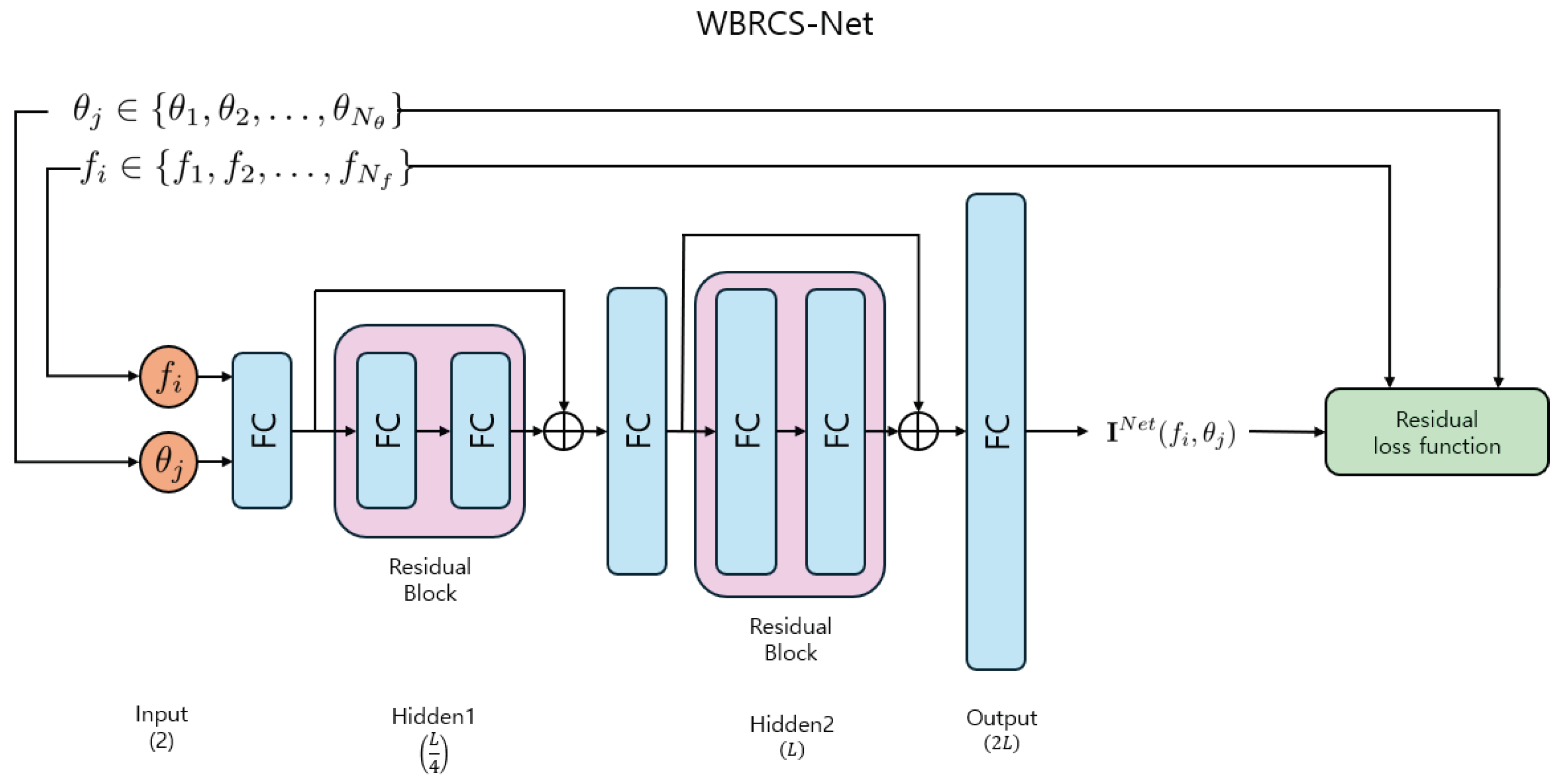
Figure 2.
Diagram of RCS computation.

Figure 3.
Two triangulated PEC objects: (a) Sphere. (b) Cube.
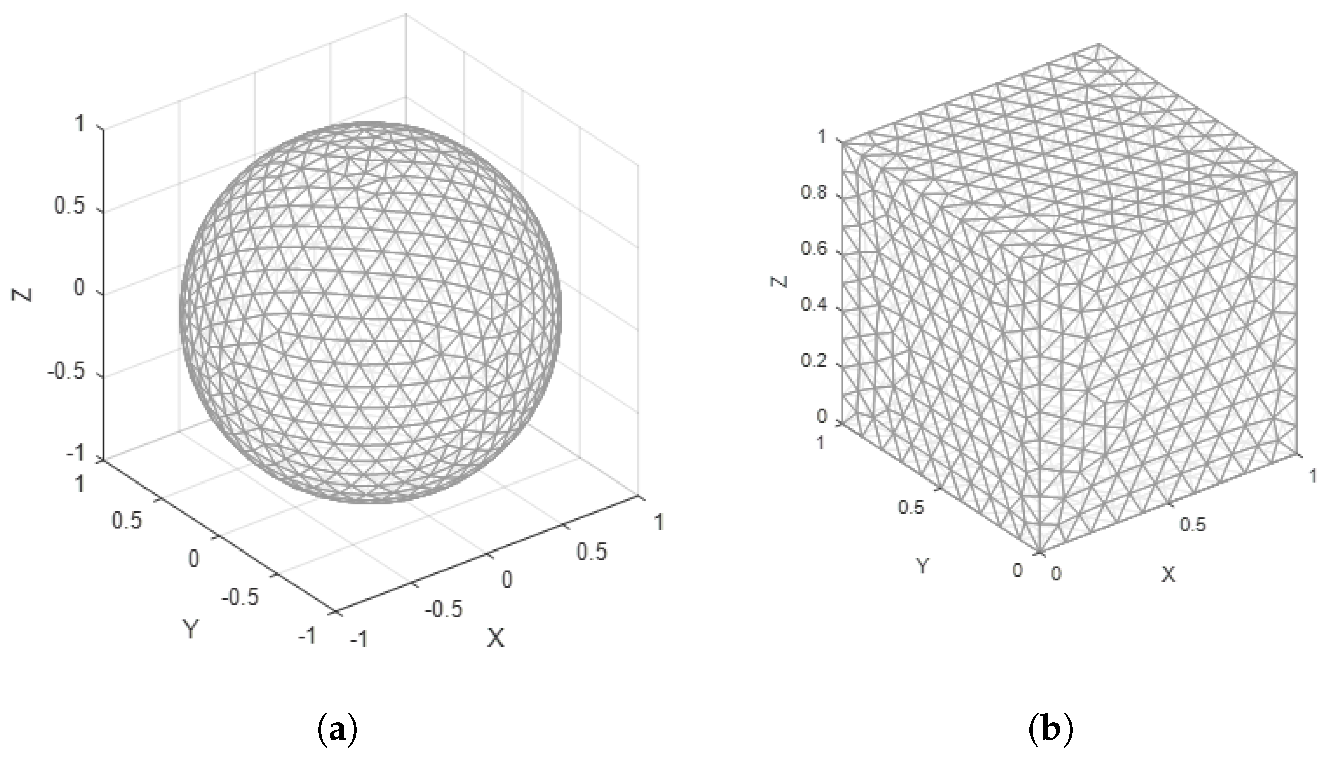
Figure 4.
Training loss over epochs.
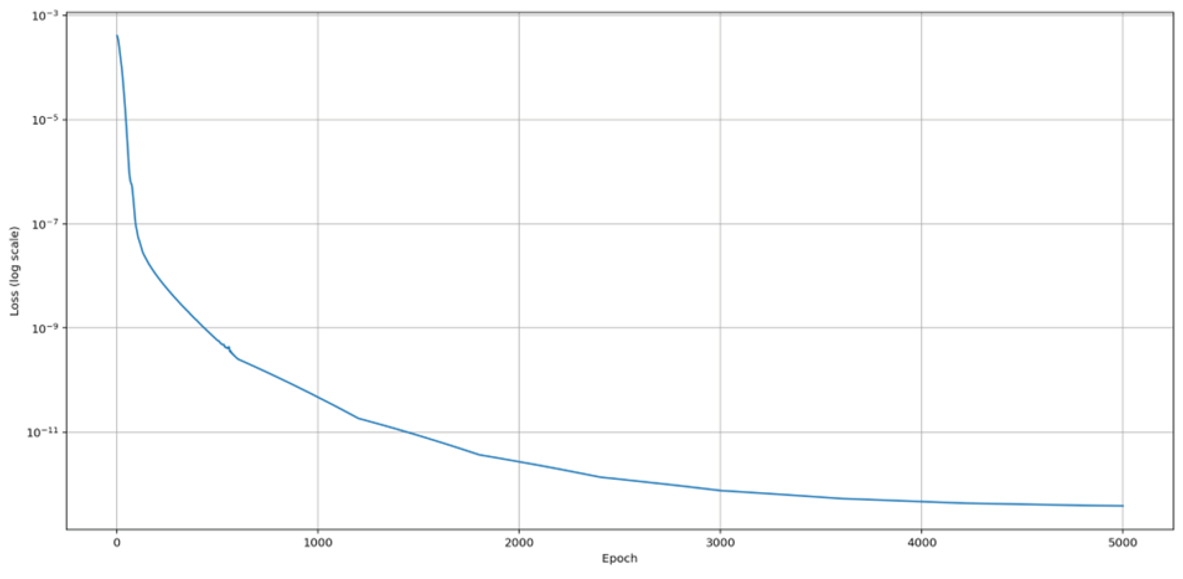
Figure 5.
Surface currents on unit sphere at 100MHz: (a) MoM. (b) WBRCS-Net.
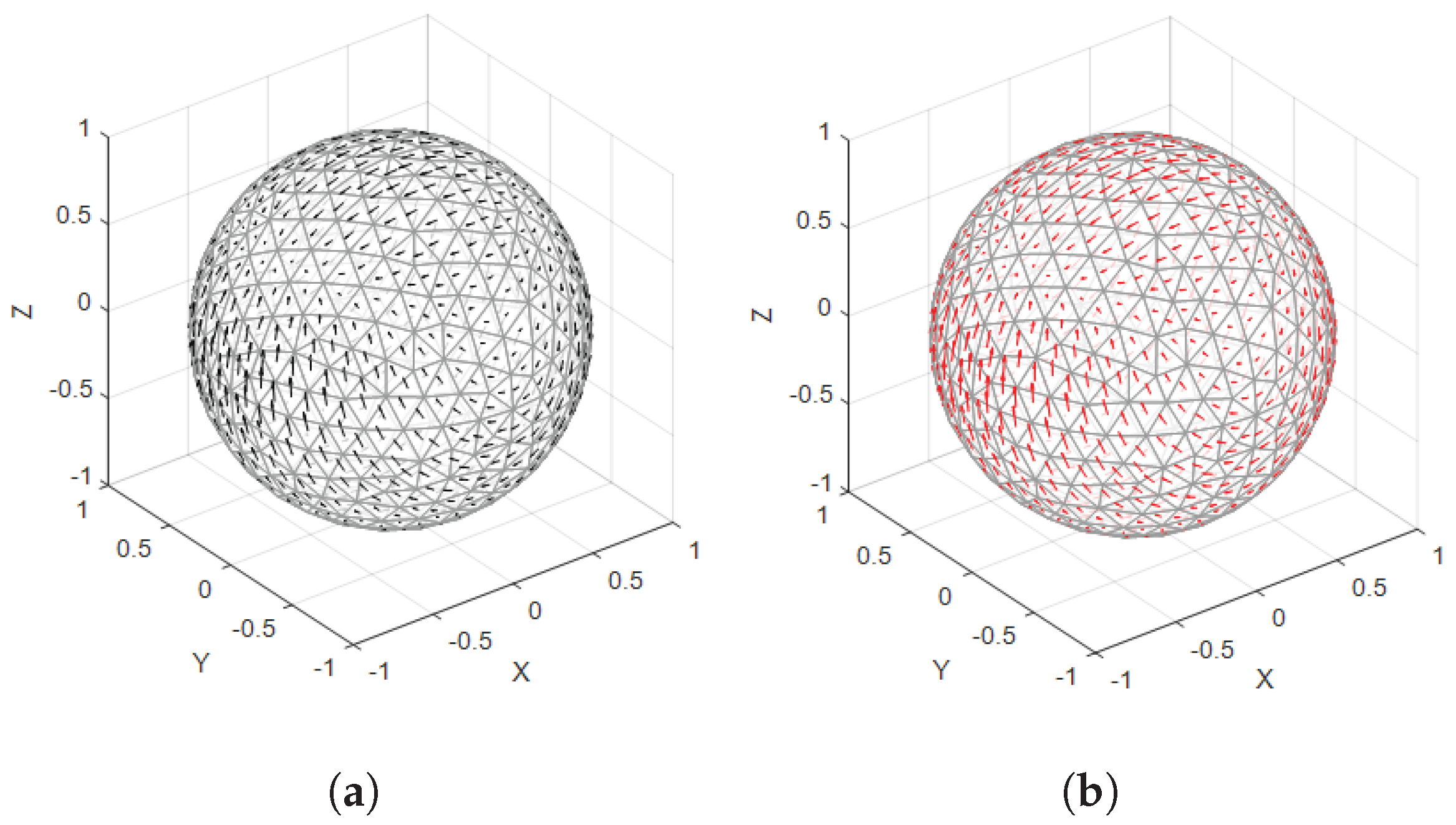
Figure 6.
Monostatic RCS on the sphere (r=3cm) with sampled points: (a) . (b) .
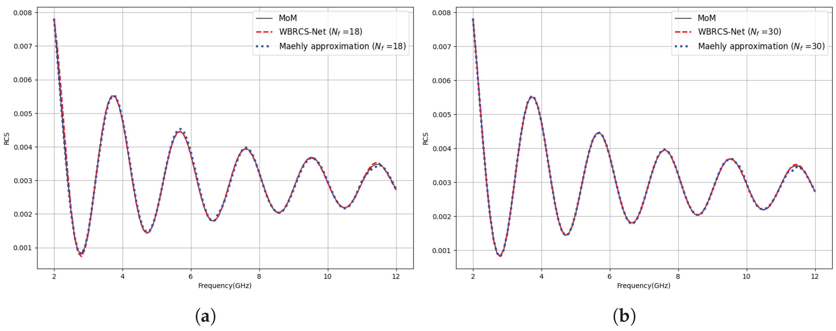
Figure 7.
Monostatic RCS on the sphere (r=4cm) with sampled points: (a) . (b) .
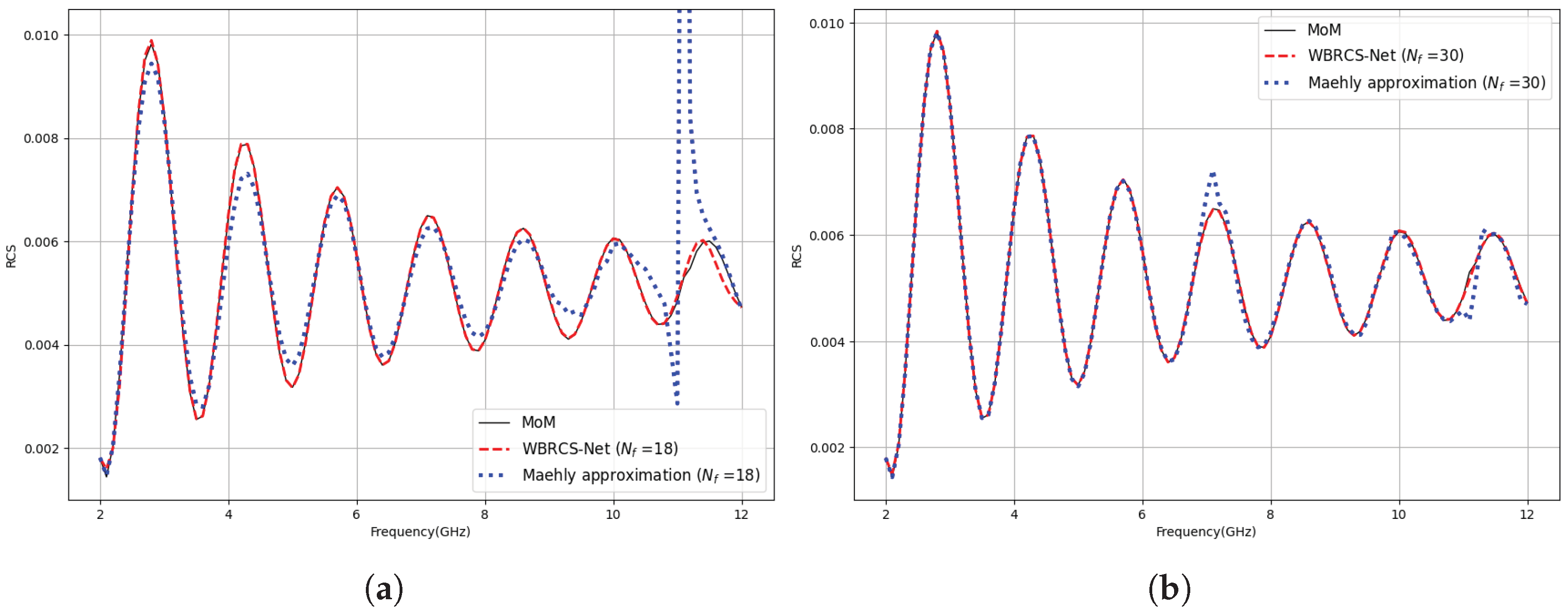
Figure 8.
MSE for each number of samples: (a) sphere(r = 3cm). (b) sphere(r = 4cm).
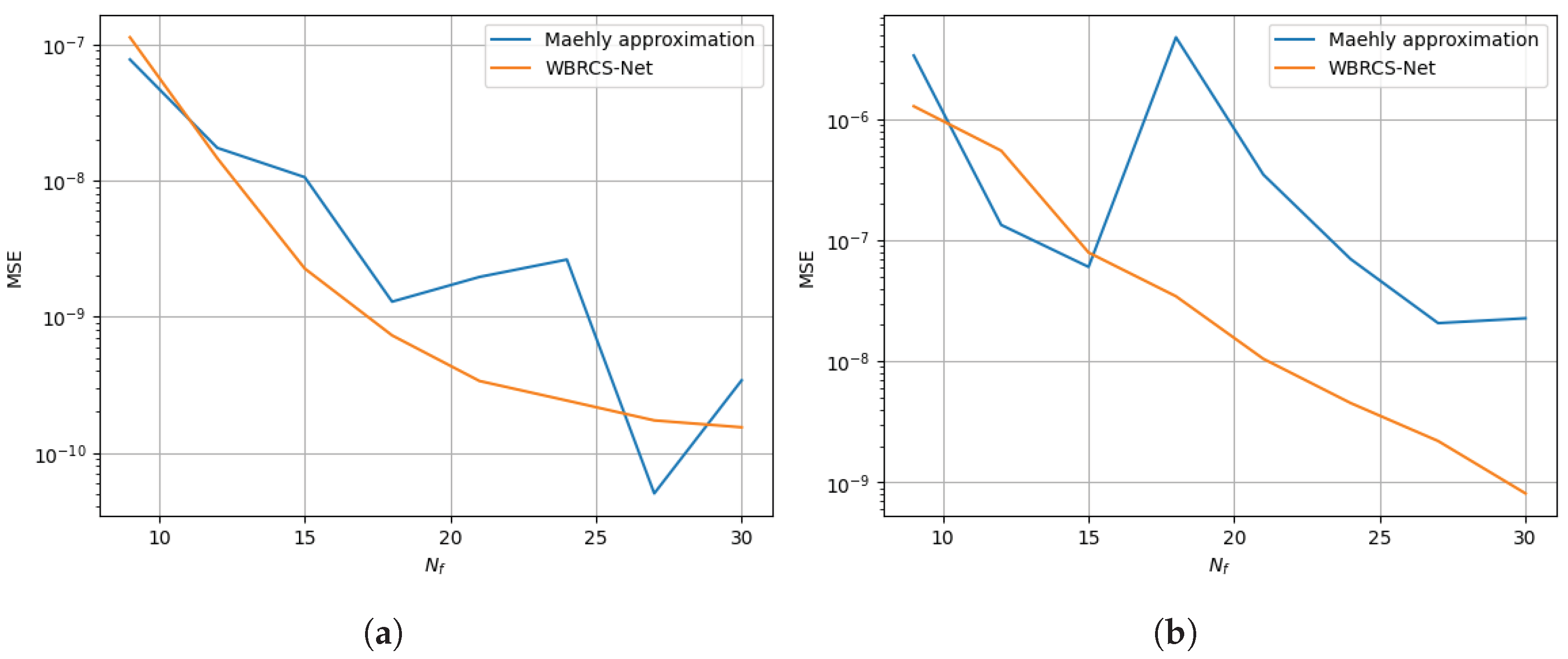
Figure 9.
Monostatic RCS on the cube (a = 3cm) with sampled points: (a) . (b) .
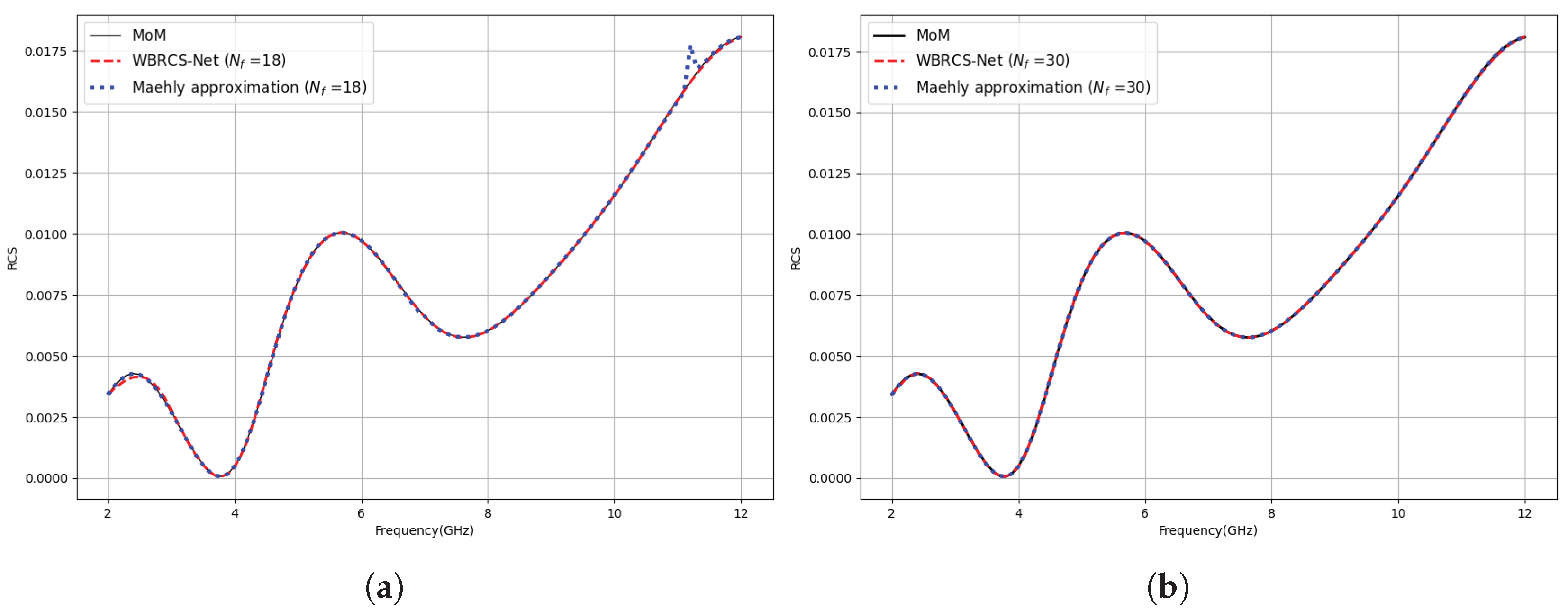
Figure 10.
Monostatic RCS on the cube (a = 6cm) with sampled points: (a) . (b) .
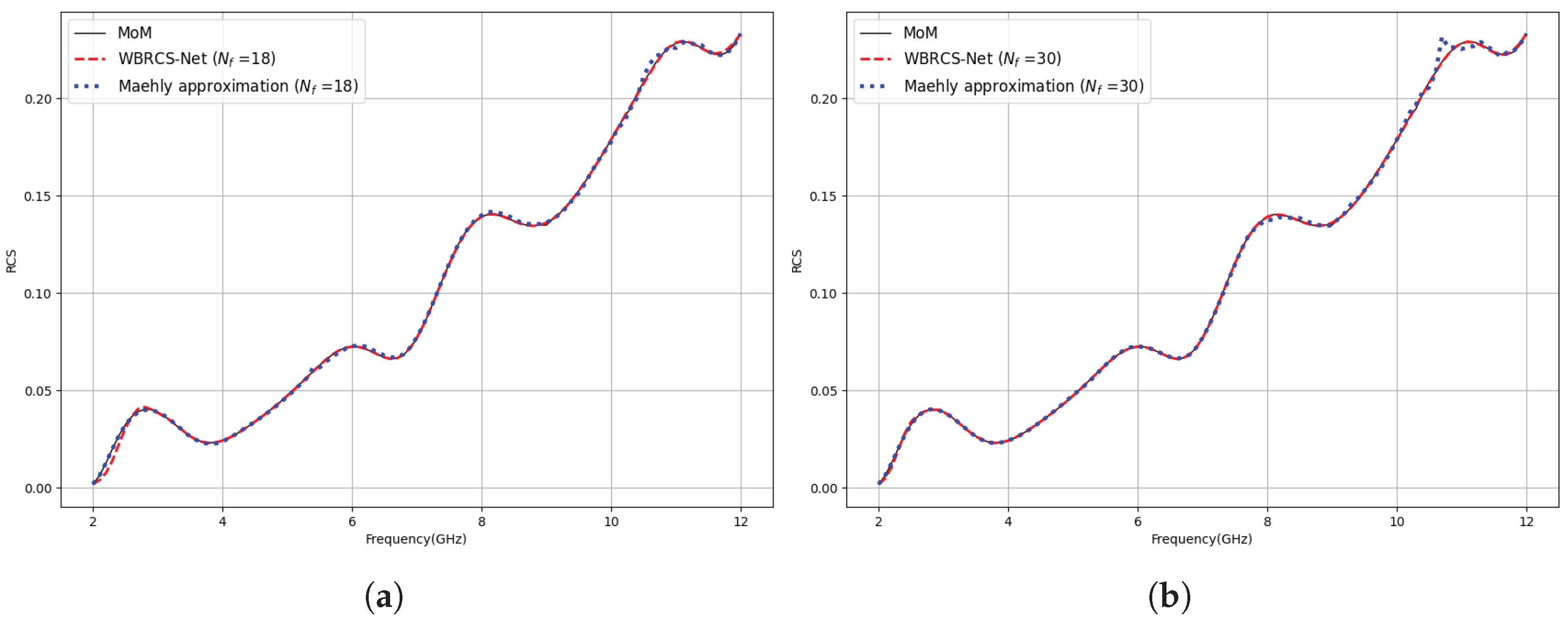
Figure 11.
MSE for each number of samples: (a) cube(a = 3cm). (b) cube(a = 6cm).
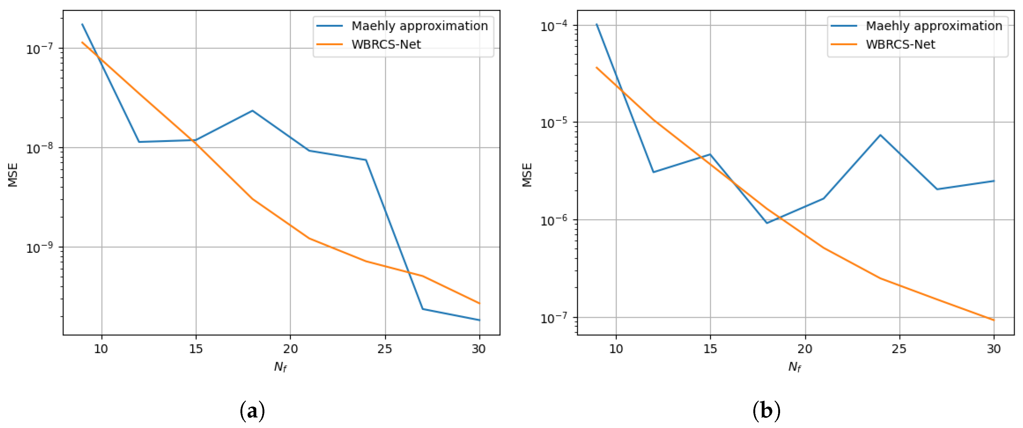
Figure 12.
3D Monostatic RCS on the cube(a = 0.5cm) predicted by WBRCS-Net
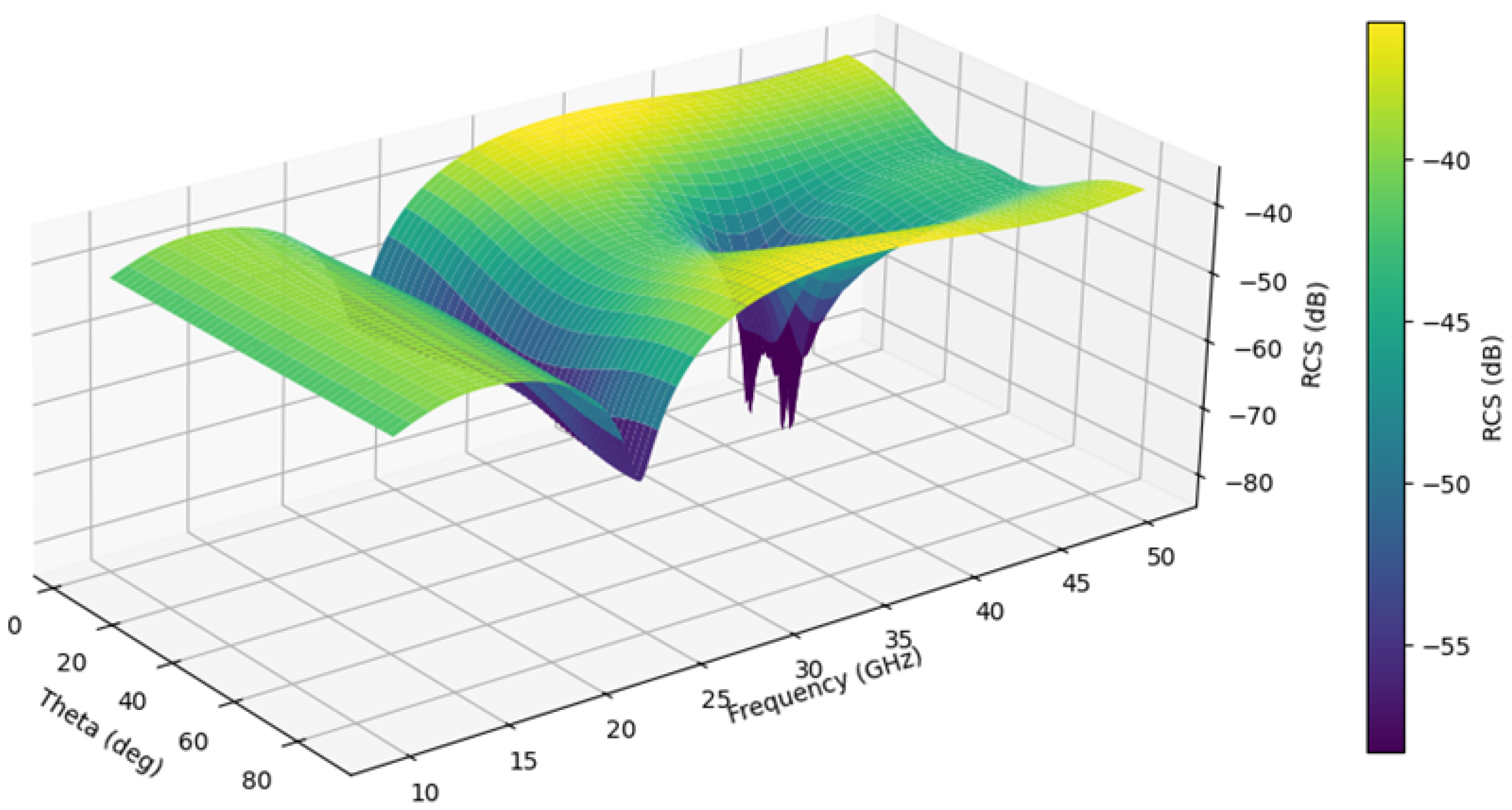
Figure 13.
Monostatic RCS on the cube (a = 0.5cm): (a) Incident angle . (b) Incident frequency f = 30 GHz.
Figure 13.
Monostatic RCS on the cube (a = 0.5cm): (a) Incident angle . (b) Incident frequency f = 30 GHz.
Disclaimer/Publisher’s Note: The statements, opinions and data contained in all publications are solely those of the individual author(s) and contributor(s) and not of MDPI and/or the editor(s). MDPI and/or the editor(s) disclaim responsibility for any injury to people or property resulting from any ideas, methods, instructions or products referred to in the content. |
© 2026 by the authors. Licensee MDPI, Basel, Switzerland. This article is an open access article distributed under the terms and conditions of the Creative Commons Attribution (CC BY) license (http://creativecommons.org/licenses/by/4.0/).
Copyright: This open access article is published under a Creative Commons CC BY 4.0 license, which permit the free download, distribution, and reuse, provided that the author and preprint are cited in any reuse.


