
Submitted:
30 January 2026
Posted:
30 January 2026
You are already at the latest version
Abstract
The cascaded liquid crystal polarization grating (CLCPG), a core non-mechanical beam scanning device, suffers from insufficient pointing accuracy due to inherent manu-facturing/assembly errors, which requires compensation by the liquid crystal optical phased array (LCOPA). Yet LCOPA is vulnerable to internal/external disturbance cou-pling and inherent time delay in practical conditions, hindering accurate compensation and limiting integrated system performance. This paper proposes a fractional-order com-posite control strategy: a fractional-order dynamic model of LCOPA is established first to characterize its response and viscoelastic memory effect; then a fractional-order mod-el-assisted extended state observer is designed for total disturbance estimation, combined with an improved Smith predictor for time-delay compensation and a phase margin method for fractional-order PID parameter tuning. Comparative experiments on a CLCPG-LCOPA experimental platform validate the strategy’s effectiveness: it suppresses disturbances, compensates CLCPG errors, reduces the overall pointing error by over 30%, improves dynamic response speed by 25%, and exhibits excellent robustness and stability, providing theoretical and technical support for high-precision CLCPG scanning system engineering.
Keywords:
cascaded liquid crystal polarization grating
; liquid crystal optical phased array
; fractional‐order composite control
; pointing error compensation
; improved smith predictor
; phase margin method
1. Introduction
The phased array lidar has emerged as a core technology in target detection [1,2], autonomous driving [3], and remote sensing imaging [4], where non-mechanical beam scanning is the key to achieving high-resolution and fast-response detection performance [5,6]. As a core component for non-mechanical scanning in phased array lidar, the cascaded liquid crystal polarization grating (CLCPG) exhibits distinct advantages of inertia-free operation and high precision [7,8,9,10], and thus plays an indispensable role in enhancing system integration and reducing the volume and weight of equipment [11,12]. The dynamic performance (e.g., scanning speed, response time) and pointing accuracy of CLCPG directly determine the imaging quality and detection efficiency of lidar systems. However, manufacturing and assembly errors are inevitably incurred during the fabrication and assembly of CLCPG, which directly result in insufficient beam pointing accuracy and necessitate dynamic compensation via the liquid crystal optical phased array (LCOPA) [13]. In practical operating conditions, LCOPA is susceptible to the combined effects of internal disturbances (e.g., viscoelastic hysteresis of liquid crystal molecules, nonlinear electro-optical response) and external disturbances (e.g., temperature fluctuations, mechanical vibration, power supply noise), and it also has an inherent time-delay characteristic superimposed on itself [14,15]. These factors render accurate compensation difficult, thereby restricting the scanning performance of the entire system. Therefore, developing a high-performance control strategy based on LCOPA compensation to address the above bottleneck issues has become the key to advancing the development of phased array lidar technology toward the high-precision field.
At present, research on beam control and error compensation of LCOPA is mainly divided into two directions: open-loop calibration optimization and closed-loop control, which provides a theoretical and technical foundation for the strategy design in this paper. Open-loop calibration optimization technology improves the pointing accuracy by correcting the corresponding relationship between the phase and the beam deflection angle. Zhou et al. [16] proposed a pattern search method to regulate the voltage distribution of adjacent electrodes to address the problem of unstable phase difference between adjacent array elements caused by voltage quantization, which further leads to different stepped heights of the outgoing light wavefront. This method effectively improves the beam pointing accuracy and reduces the system error by two orders of magnitude. Qiao [17] adopted a phase iterative compensation method to enhance the pointing accuracy of the LCOPA beam control system, which compensates the quantized voltage of each array element of the LCOPA to obtain the optimal voltage value and thus correct the phase delay. Wang et al. [18] proposed an improved beam control method with periodic phase distribution, which maintains a good linear relationship between the driving voltage and the phase, thereby improving the beam pointing accuracy and achieving a precision error of less than 5 urad for beam scanning with constant angular resolution. Niu et al. [19] solved the director distribution of liquid crystal molecules by using the nonlinear least square method, established a more accurate electro-optical control characteristic curve of the LCOPA, obtained a precise corresponding relationship between phase and voltage, and significantly improved the beam pointing accuracy with an average pointing accuracy error of 0.0098° within the beam scanning range. Zeng et al. [20] developed a digital holographic measurement and calibration technology, reducing the nonlinear error of the LCOPA response to 2.45%. Zhang et al. [21] revealed the dynamic beam deflection law in depth by establishing the dynamic response and far-field diffraction model of the LCOPA, which provides important theoretical support for high-precision control. In the research of closed-loop control strategies, scholars have carried out extensive explorations focusing on the objectives of disturbance rejection and response speed improvement. Orzechowski et al. [22] proposed a closed-loop beam control method for the LCOPA and designed a variable-order adaptive controller based on a recursive least square filter, which achieved high deflection accuracy within the deflection range. This method effectively suppresses the disturbances of the LCOPA beam control system and enhances the system robustness. Du [23] designed an LCOPA beam control system based on a PI controller, which effectively improves the system response speed and suppresses external disturbances. Li et al. [24] designed a fractional-order PID controller for LCOPA beam control. Experimental results show that compared with the traditional integer-order PID controller, this scheme can shorten the dynamic adjustment time of the system by more than 30% and reduce the steady-state error by 45%, which effectively improves the dynamic response characteristics and error suppression capability of the system. Xu et al. [25] proposed a PID tracking method for space laser communication based on the LCOPA, which realizes the agile deflection of the incident beam to achieve the tracking purpose. Fan [26] adopted a BP neural network PID control strategy and built a closed-loop LCOPA beam control system, which can adaptively adjust its own parameters and improve the stability and anti-interference ability of the system. Wang [27] proposed a three-step control method for the beam deflection control problem of the LCOPA, aiming to achieve fast, accurate and stable beam deflection.
Despite the phased progress achieved in existing research on pointing accuracy optimization and nonlinear error suppression, two critical gaps remain in meeting the practical high-precision scanning requirements of CLCPG. First, most existing control strategies focus on improving a single performance index (e.g., pointing accuracy) and fail to realize the coordinated optimization of dynamic response speed and pointing accuracy, making it difficult to match the dual demands of fast response and high precision. Second, in the face of the combined internal and external disturbances and inherent time-delay characteristics of LCOPA, existing schemes have limited capabilities in disturbance observation and compensation, leading to insufficient system robustness. Fractional-order composite control integrates the high-precision dynamic regulation characteristics and the advantage of adaptive disturbance compensation of fractional-order control, which can effectively handle complex systems with nonlinearity, strong coupling and multiple disturbances, thus providing an ideal technical approach to address the above problems.
To this end, a fractional-order composite control strategy is proposed in this paper. By precisely controlling the LCOPA, the strategy drives it to efficiently compensate for the pointing error of the CLCPG. The specific research work is as follows: First, an error compensation system for CLCPG is designed, and a fractional-order dynamic nominal model of LCOPA is established to accurately characterize its response law and viscoelastic memory effect. Subsequently, a fractional-order model assisted extended state observer (FMAESO) is designed, which combines the model parameters of LCOPA to accurately estimate the total disturbance and realize real-time feedback. Based on the observation results, a fractional-order composite control law is designed to drive LCOPA to output a disturbance-adaptive compensation amount for correcting the CLCPG deviation. Meanwhile, an improved Smith predictor is introduced to compensate for the system time delay, thus constructing a complete control architecture. Then, the parameters of the fractional-order PID (FOPID) controller are tuned based on the phase margin method to ensure the compensation accuracy of LCOPA, achieving fast, accurate and stable beam pointing of the overall system. Finally, an optical experimental platform integrating CLCPG and LCOPA is built, and the effectiveness of the proposed control strategy is verified through comparative experiments. The results show that the proposed strategy can effectively suppress the influence of working condition disturbances on the beam pointing accuracy of LCOPA and efficiently compensate for the manufacturing and assembly errors of CLCPG. Compared with the traditional control scheme, the overall beam pointing error of the system is reduced by more than 30%, the dynamic response speed is increased by 25%, and the system exhibits excellent robustness and stability simultaneously. This research provides an important theoretical basis and technical support for the engineering implementation of high-precision CLCPG scanning systems.
2. Design and Dynamic Characteristic Analysis of the LCOPA Compensation System
2.1. Design of the Coarse-Fine Two-Stage Compensation System for the LCOPA
The CLCPG enables discrete beam steering with a large angle and high diffraction efficiency [28]. To achieve multi-angle scanning and expand the steering range, a cascaded system is formed by the alternating arrangement of multiple liquid crystal polarization gratings (LCPG) and circular polarization switches. The circular polarization switch dynamically reverses the handedness of circularly polarized light, while the liquid crystal polarization grating deflects circularly polarized light with different handedness to distinct directions. These two components complement each other to realize dynamic beam scanning, and its structure is shown in Figure 1.
However, limited by manufacturing and assembly processes, the deflection angles of LCPG exhibit inherent errors, with the error magnitude increasing as the number of cascaded gratings rises. For this reason, the CLCPG is regarded as a coarse beam steering system for large-angle beam control. In contrast, the LCOPA features high resolution, continuous deflection and programmable logic control, enabling high-precision beam steering within a small angular range, and is thus defined as a fine beam steering system. By combining the advantages of LCPG and LCOPA, the fine steering system is used to compensate for the beam pointing errors of the coarse steering system, achieving large-angle, high-precision, fast and stable beam steering. The corresponding compensation system is illustrated in Figure 2.
2.2. Modeling and Dynamic Characteristic Analysis of the LCOPA
The LCOPA generates a phase difference by regulating the voltage distribution between adjacent electrodes, forming a wavefront with a phase modulation amount of . The driving voltage corresponding to the wavefront is calculated according to the liquid crystal phase regulation characteristic curve, and then the voltage is converted into a grayscale image using a linear voltage lookup table (LUT), which is loaded onto all electrodes of the LCOPA. Driven by the driving voltage, the birefringence of liquid crystal molecules changes, thereby realizing the phase regulation of the incident light beam and achieving beam deflection [29,30]. Starting from the viscoelastic characteristics of the liquid crystal molecular deformation of the LCOPA, this paper constructs a dynamic equilibrium equation of liquid crystal molecules in a single array element based on the fractional-order Kelvin model. Combined with the idea of the microwave phased array radar, a dynamic model between the phase difference of the LCOPA and the beam deflection angle is established, which is expressed as follows:
 where: is the volume charge distribution coefficient, is the time-delay coefficient of the system, is the element width of the LCOPA, is the viscosity coefficient of the splay deformation, is the fractional order of the splay deformation, is the viscosity coefficient of the bend deformation, is the fractional order of the bend deformation, and are the elastic coefficients of the splay deformation and bend deformation, respectively.
By building an optical experimental platform to collect the angular data during the dynamic beam deflection process, the fractional-order model of the LCOPA identified via the system identification method is expressed as follows:
Then, the dynamic response characteristic curves of the integer-order and fractional-order models during the power-on and power-off phases of the LCOPA were compared and analyzed when the phase difference , as shown in Figure 3 and Figure 4 below.
It can be seen from Figure 3 that when the applied phase difference is , the beam deflection angle gradually shifts from 0 rad to 0.0272 rad. The fractional-order model established in this paper can well characterize the dynamic performance of beam deflection with a fitting degree of 98%, whereas the integer-order model exhibits a large fitting error with the actual data. As shown in Figure 4, after the voltage is removed, the beam deflection angle gradually returns from 0.0272 rad to 0 rad, and the fractional-order model can also accurately simulate the power-off process, which verifies the effectiveness of the proposed fractional-order model. Furthermore, the response characteristics of the integer-order and fractional-order models of the LCOPA at different frequency bands are simulated and analyzed in the frequency domain, with the simulation results presented in Figure 5. It can be observed from the amplitude-frequency characteristic curves that the fractional-order model has a slower amplitude attenuation and a slightly larger bandwidth (1.3 rad/s) than the integer-order model, indicating that the fractional-order model can better match the viscoelastic dynamic response of the liquid crystal. From the phase-frequency characteristic curves, the fractional-order model features a lower phase delay, a smaller beam pointing error and better system stability, with its phase margin close to 60°.
3. Design of the Fractional-Order Composite Controller
In practical operating conditions, the LCOPA is susceptible to the combined effects of internal and external disturbances such as voltage quantization, liquid crystal cell surface unevenness, pixel crosstalk, phase dips and hysteresis zones. Coupled with the inherent time-delay characteristics of the system in transmission and data processing links, it is difficult to achieve accurate compensation for CLCPG errors, which in turn restricts the performance improvement of the entire scanning system. To address this issue, a composite fractional-order controller is designed in this paper based on the fractional-order model of the LCOPA, which realizes high-efficiency compensation for the pointing accuracy of the CLCPG through the high-precision control of the LCOPA. The composite fractional-order controller consists of a modified Smith predictor, a FMAESO and a FOPID controller. Among them, the modified Smith predictor is specially used to compensate for the time-delay caused by system transmission and data processing, thus improving the dynamic response characteristics of the system; the FAMESO integrates the a priori information of the LCOPA fractional-order model to realize real-time and accurate observation of multi-source composite disturbances including voltage quantization and pixel crosstalk, and complete adaptive compensation for such disturbances; the FOPID controller utilizes the flexible regulation characteristics of fractional-order calculus to achieve refined adjustment of the dynamic response process of the system, which significantly enhances the dynamic response performance of the system. The structure of the composite fractional-order control system for the LCOPA is shown in Figure 6.
3.1. Design of the Improved Smith Predictor
Before the Smith predictor is incorporated into the system, the closed-loop transfer function between the system input and output is expressed as follows:
From the above equation, it can be seen that the characteristic equation contains a time-delay term . When the system output is fed back to the controller, and the controller then outputs the adjustment signal, the presence of this delay may prevent the controller from responding promptly to changes in the system state, which can lead to oscillations or instability. Therefore, a Smith predictor is introduced to mitigate the impact of time delay on the system’s dynamic performance, as shown in Figure 7 below.
In the figure above, is the system input, is the FOPID controller, is the controlled plant with a pure time-delay element, is the time-delay factor of the controlled plant, is the prediction model with the pure time-delay element removed, is the time-delay factor of the prediction model, and is the system output.
At this point, the closed-loop transfer function between the system input and output is given as follows:
It can be seen from Equation (4) that, under ideal conditions, when the model is perfectly matched (i.e., and ), the closed-loop transfer function is transformed into:
It can be concluded from the above equation that there is no time-delay term in the characteristic equation, such that the control performance of the system can respond in a timely manner and the control quality of the system is thus improved.
Smith predictive compensation strategy can eliminate the influence of pure time delay on the control system. However, the conventional Smith predictive compensator has poor anti-interference capability. During the operation of the LCOPA, factors such as ambient temperature fluctuations and changes in the viscoelasticity of the liquid crystal layer are likely to introduce certain errors into the system model. The existence of such errors will lead to a significant degradation in the compensation performance of the conventional Smith predictive compensator and may even result in system instability. Therefore, the conventional Smith predictive compensation strategy is improved, and the structure of the improved Smith predictive compensator is shown in Figure 8 below.
In the figure above, is the filter time constant of the system, is the estimated output of the system with the pure time-delay element removed, and is the output of the deviation between the estimated system output with the pure time-delay element and the actual output after passing through a first-order filter. As can be seen from Figure 8, after the improved Smith predictive compensator is applied, the closed-loop transfer function between the system input and output is given as follows:
Under ideal conditions, when the prediction model is perfectly matched with the controlled plant (i.e., and ), the situation is consistent with Equation (5). When there is a mismatch between the prediction model and the controlled plant, the closed-loop feedback signal is derived from the output signal and the output signal of the prediction model. Thus, the improved Smith predictive compensator can adjust part of the feedback signal by tuning the filter time constant, thereby enhancing the anti-interference capability and stability of the system.
From the above analysis, it can be concluded that the designed improved Smith predictor can eliminate the time-delay term in the system. Therefore, the fractional-order model of the LCOPA can be rewritten in the following time-delay-free form:
3.2. Design of the FMAESO
After compensating for the system time delay with the improved Smith predictor, the LCOPA is still subject to the effects of combined internal and external disturbances, including nonlinear factors such as voltage quantization errors, temperature drifts, and viscoelastic hysteresis of liquid crystal materials. To achieve high-precision observation and compensation of the total disturbance, a FMAESO is designed in this section based on the fractional-order dynamic model of the LCOPA established in Section 2.2. This observer uniformly models the system dynamic characteristics and external disturbances as an extended state, and realizes real-time estimation and feedforward compensation through output feedback, thereby improving the anti-disturbance performance and control accuracy of the system.
The fractional-order model of the LCOPA considering the total disturbance can be rewritten as follows:
Further organize into:
where: denotes the fractional differential operator, is the fractional order, and are the fractional dynamic coefficients, and are the input and output of the controlled plant, respectively, is the total disturbance term, which includes system dynamics, order discrepancies, and unknown disturbances, and is the nominal control gain.
To construct the FMAESO, the following extended state variables are defined:
Among them, represents the beam deflection angle of the LCOPA, is the -order derivative of the output, reflecting the viscoelastic dynamic change rate of liquid crystal deformation, and is the extended state, i.e., the total disturbance. Based on this, the fractional-order state-space equation of the system is established as follows:
Its matrix form is:
Among them
The FMAESO estimates the state variables and the total disturbance in real time through output feedback, and its observer equation is:
The matrix form is:
where: is the observer gain matrix, and is the state estimation vector. The observer gain matrix is obtained through observer pole placement calculation.
where: is the observer bandwidth. Based on the analysis of the dynamic characteristics of the controlled plant, is set to 6rad/s to balance the estimation speed and anti-interference performance.
The estimated total disturbance is used for feedforward compensation, and the overall control rate is designed as:
where: is generated by the FOPID controller based on the tracking error .
The frequency domain expression is
where: is the proportional gain, is the differential gain, is the integral gain, and are the fractional orders.
The designed FMAESO is shown in Figure 9. This FMAESO structure assists state estimation using model prior information, which significantly improves the observation accuracy and response speed, and provides a reliable disturbance observation basis for subsequent composite control.
3.3. Design of the Fractional-order Controller
It can be seen from the design process of the FOPID controller that the parameters of the fractional-order error feedback control rate, , and , are unknown. Therefore, this paper starts from the frequency-domain characteristics of the LCOPA system and adopts the phase margin method to calculate the controller parameters. The open-loop transfer function of the designed LCOPA system is , and the phase margin at the system’s open-loop crossover frequency is . Thus, performing the fractional-order Laplace transform on Equation (1) yields the following fractional-order transfer function form:
Let and , then the transfer function of the phased array control system can be simplified as:
Since the phase and system damping of the LCOPA system are interrelated, phase margin should be treated as a key criterion in the design of the fractional-order controller for the relative stability of the control system. Based on the desired characteristics of the phased array in application, by specifying the phase margin and cutoff frequency of the phased array system, the following parameter tuning rules for the FOPID controller can be obtained:
The magnitude at the crossover frequency on the magnitude-frequency characteristic curve of the system open-loop transfer function satisfies:
The phase at the crossover frequency on the phase-frequency characteristic curve of the system open-loop transfer function satisfies:
The phase of the system open-loop transfer function satisfies the following relation:
The open-loop transfer function and open-loop frequency response of the LCOPA system based on the FOPID controller are:
From this, we can obtain the phase and magnitude characteristics of the system open-loop transfer function . Furthermore, based on the tuning rules (21), (22), and (23) for the fractional-order controller parameters in this paper, the following controller parameter relations are derived:
Among them
Since the FOPID controller has two additional tuning parameters and , to solve for the five parameters , , , and , an optimization function approach is required in addition to the three parameter tuning rules (21), (22), and (23). The fmincon function in the MATLAB optimization toolbox is used to solve these nonlinear equations. Equation (27) is selected as the main minimization function, and by combining Equations (26), (27) and (28), the parameters of the FOPID controller can be obtained. To ensure strong stability and robustness of the beam steering system, the system is designed with a bandwidth =2.4rad/s and a phase margin . The calculated parameters are , , , and . Thus, the transfer function model of the FOPID controller is:
4. Simulation Analysis
To verify the control performance of the designed fractional-order composite controller, a comparison is made with the PID controller and the FOPID controller. The PID parameter tuning toolbox in MATLAB/Simulink is used to tune the controller parameters, yielding the optimal PID controller parameters as: , , .
4.1. Step Response Test
The deflection angle of the beam precision control system for the liquid crystal optical phased array was set to 1∘, and the step response performances of the three controllers were compared, with the comparison results recorded in Table 1. Figure 10(a) and Figure 10(b) show the step response and error comparison results, respectively. It can be seen from the figures that both the response speed and control accuracy of the fractional-order composite controller designed in this paper are superior to those of the other two controllers. The system reaches a steady state at 8.84 ms without overshoot, while the response times of the FOPID and PID controllers are 30.25 ms and 42.18 ms, respectively, with a certain overshoot for both. The ITAE performance index also fully demonstrates that the fractional-order composite controller has the minimum ITAE value, and the index of the FOPID controller is lower than that of the PID controller. This verifies that the fractional-order controller exhibits better control performance for fractional-order systems.
4.2. Dynamic Beam Variation Performance Test
The beam deflection angle of the LCOPA beam precision control system changes continuously during actual operation. Therefore, to verify whether the designed controller can rapidly regulate the beam deflection angle to enable fast and accurate tracking of the variation in the target trajectory, verification tests were conducted in accordance with three operating modes of the beam control system: polyline scanning, continuous scanning and fixed-point switching. First, the polyline scanning mode was verified: the beam started at , deflected to with a step of and a step interval of 50 ms, and then scanned back from to . Second, the continuous scanning mode was verified, where the beam was driven to vary continuously between and . Finally, the fixed-point switching mode was verified, in which the beam deflection angle was switched mutually between and with a period of 100 ms. The dynamic tracking results of the target trajectory are shown in Figure 11, Figure 12 and Figure 13.
It can be seen from the above figures that the method proposed in this paper exhibits excellent tracking performance for beam trajectory variations under all operating modes, with fast tracking speed and small tracking errors. In contrast, although the PID and FOPID controllers are also able to track target changes, their tracking performance is poor, characterized by long dynamic adjustment times and large tracking errors.
4.3. Robustness Test
The beam pointing of the LCOPA beam precision control system may mutate due to carrier vibration or external disturbances. To simulate the process of abrupt disturbance, a step signal with an amplitude of was added to the output position to mimic external disturbances when the system reached a steady state. The dynamic response of the system under external disturbances is shown in Figure 14. It can be seen from the figure that the PID and FOPID controllers exhibit a slow adjustment speed to disturbances, while the fractional-order composite controller can effectively regulate the beam deflection angle and restore the system to a steady state rapidly.
Due to temperature variations and device aging, the model parameters of the LCOPA beam precision control system will change. Therefore, it is assumed that the model parameters and vary within ±10%, as shown in the table. Similarly, the orders of the fractional-order model and are also varied within ±10%, and the control system performance is illustrated in Figure 15, Figure 16 and Figure 17. The results indicate that the designed fractional-order composite controller exhibits strong robustness. Whether the system model parameters change or the model order varies, it can effectively regulate the LCOPA to maintain the stability of the beam pointing.

Table 2.
Parameters of the fractional-order model for the beam precision control system.
| Model | b | ||||||
|---|---|---|---|---|---|---|---|
| G1 | 80.37 | 75.97 | 28.20 | 0.50 | 1.8 | 0.9 | 3.027 |
| G2 | 76.72 | 72.51 | 28.20 | 0.50 | 1.8 | 0.9 | 3.027 |
| G3 | 73.07 | 69.06 | 28.20 | 0.50 | 1.8 | 0.9 | 3.027 |
| G4 | 69.41 | 65.61 | 28.20 | 0.50 | 1.8 | 0.9 | 3.027 |
| G5 | 65.76 | 62.16 | 28.20 | 0.50 | 1.8 | 0.9 | 3.027 |
Next, the gain robustness of the controller is verified. The gain of the fractional-order error feedback control law, the integral order and the differential order are varied within ±10% respectively, with the control effects shown in Figure 18, Figure 19 and Figure 20. It can be seen from the figures that when the gain and orders of the fractional-order error feedback control law change, the dynamic performance of the beam pointing exhibits minimal variation. This is because the fractional-order model auxiliary extended state observer in the fractional-order composite controller plays a primary regulatory role, while the fractional-order error feedback control performs auxiliary adjustment within a small error range, serving to eliminate steady-state errors and suppress disturbances. Therefore, this further verifies that the designed controller has strong robustness.
5. Experimental Verification
To verify the effectiveness of the designed coarse-fine two-stage synchronous control system for the LCOPA, a hardware-in-the-loop simulation platform based on LabVIEW was developed for validation. First, the fractional-order composite controller was discretized using the Oustaloup method and numerically implemented on LabVIEW. Second, the data interaction between the LCOPA, high-speed CCD camera and LabVIEW were realized via dynamic link library (DLL) calling: the LCOPA was controlled by LabVIEW for beam deflection through a PCIE interface, and the high-speed CCD camera was used by LabVIEW for data acquisition of the light spot deflection angle through an Ethernet interface. Finally, the experimental platform as shown in Figure 21 was built to verify the response speed, beam pointing accuracy and disturbance rejection capability of the system.
5.1. System Response Speed
In the coarse-fine two-stage synchronous control system for the LCOPA, the response speed of the LCOPA is faster than that of the CLCPG; therefore, the beam pointing speed of the LCOPA determines the system’s response speed. To verify whether the designed fractional-order composite controller can effectively improve the response speed of the LCOPA, the response speeds of the LCOPA with and without the fractional-order composite controller were compared. First, the beam pointing angle of the fine control system was set to , and the beam pointing angle of the coarse control system was set to . Second, the system was operated, and the fractional-order composite controller was used to regulate the beam pointing. Finally, the image processing system was employed to record the change process of the light spot centroid and convert it into the actual deflection angle. The comparison results are shown in Figure 22.
It can be seen from the comparison results that the designed fractional-order composite controller can effectively improve the response speed of the system. With the fractional-order composite controller incorporated, the beam pointing reaches a steady state at 10 ms; in contrast, the system does not achieve stability until 14 ms without the controller. Thus, it is verified that the designed fractional-order composite controller can effectively enhance the response speed of the coarse-fine two-stage synchronous control system for the LCOPA, with the response speed improved by 28.57%.
5.2. System Pointing Accuracy
To verify the beam pointing accuracy of the coarse-fine two-stage synchronous control system for the LCOPA, the triangulation method was adopted to obtain the actual deflection angle of the beam, which was then compared with the theoretical value to derive the beam pointing error. In addition, the beam pointing accuracy before and after the incorporation of the fine control system was compared to validate the accuracy compensation performance of the fine control system. First, a laser rangefinder was used to measure the distance between the high-speed CCD camera and the light screen as 0.82 meters. Second, the fine control system was deactivated, and only the CLCPG were regulated to deflect the beam from to with an angular resolution of . Finally, the image processing system was employed to calculate the offset of the light spot centroid and convert it into the actual beam pointing angle. To ensure the accuracy of the calculations, the displacement of the light spot centroid was measured 100 times for each deflection angle, and the average value was taken. The results are recorded in Table 3, and the beam pointing errors are shown in Figure 23.
Figure 23 shows that a considerable error exists between the actual beam pointing and the theoretical value when the fine control system is not in operation. This is because the period of the LCPG is difficult to match the theoretical value due to manufacturing and assembly errors, which further leads to errors in the beam deflection angle; in addition, the more gratings are cascaded, the larger the error becomes. The root mean square error (RMSE) is used to characterize the beam pointing accuracy, and the RMSE of the system is 0.0185. The fine control system was then operated synchronously with the coarse control system to compensate for the beam pointing error of the coarse control system, with the results recorded in Table 4. The comparison results of the beam pointing error before and after the operation of the fine control system are presented in Figure 24. It can be seen from the figure that the LCOPA can effectively compensate for the beam pointing error of the coarse control system; the RMSE after compensation is 0.0066, which is a reduction of 0.0119 compared with that before compensation.
5.3. System Robustness
Finally, the disturbance rejection capability of the coarse-fine two-stage synchronous control system for the LCOPA was verified. First, the beam deflection angle was set to . Then, an external disturbance of was applied to the system when it reached a steady state. Finally, the offset of the light spot centroid was calculated via the image processing system and converted into the deflection angle to verify whether the system could regulate the beam pointing rapidly and accurately. The beam regulation results are shown in Figure 25.
It can be seen from the figure that in the face of external disturbances, the fractional-order composite controller can effectively regulate the beam deflection angle, enabling it to quickly return to the set value and achieve fast, accurate, and stable beam regulation. Thus, it is further verified that the coarse-fine two-stage synchronous control system for the LCOPA designed in this paper has strong robustness.
6. Discussion
Aiming at the problem that the performance of the CLCPG system is restricted by the composite disturbances and time-delay effects of the LCOPA, this paper conducts the research on the fractional-order composite control strategy. First, a fractional-order model of LCOPA integrating the viscoelastic memory effect and disturbances is established, which accurately characterizes its nonlinear characteristics. Second, a composite control strategy based on the FMAESO is proposed, which combines the FOPID with the improved Smith predictor to realize the collaborative optimization of dynamic response and pointing accuracy. Finally, the phase margin method and numerical optimization are adopted to tune the parameters, which solves the problem of multi-parameter tuning for the fractional-order controller. Experimental verification results show that the step response time of the proposed composite control strategy is 8.84 ms with the pointing error ≤. Compared with the traditional scheme, the pointing error of the CLCPG system is reduced by 30%, the response speed is increased by 25%, and the system exhibits excellent anti-disturbance performance. The research results can provide technical support for the engineering application of the CLCPG system and can be extended to other similar nonlinear systems. In the future, the research will focus on optimizing the performance of the observer, developing the controller for complex working conditions, and promoting the hardware implementation of the proposed control strategy.
Author Contributions
Conceptualization, M.T. and J.Y.; methodology, M.T.; software, M.T.; validation, M.T., J.Y. and J.J.; formal analysis, X.L.; investigation, M.T.; resources, M.T.; data curation, J.Y.; writing—original draft preparation, M.T.; writing—review and editing, C.W.; visualization, M.T.; supervision, J.J.; project administration, C.W. All authors have read and agreed to the published version of the manuscript.
Funding
This research received no external funding.
Data Availability Statement
Not applicable
Acknowledgments
The manuscript was supported by the Xi’an Key Laboratory of Active Optoelectronic Imaging Detection Technology. This research did not receive any specific grant from funding agencies in the public, commercial, or not-for-profit sectors.
Conflicts of Interest
The authors declare no conflicts of interest.
References
- Xie, D.; Wang, X.; Wang, C.; Yuan, K.; Wei, X.; Liu, X.; Huang, T. A Fractional-Order Total Variation Regularization-Based Method for Recovering Geiger-Mode Avalanche Photodiode Light Detection and Ranging Depth Images. Fractal Fract. 2023, 7, 445. [Google Scholar] [CrossRef]
- Wei, X.; Wang, C.; Xie, D.; Yuan, K.; Liu, X.; Wang, Z.; Wang, X.; Huang, T. Fractional-Order Total Variation Geiger-Mode Avalanche Photodiode Lidar Range-Image Denoising Algorithm Based on Spatial Kernel Function and Range Kernel Function. Fractal Fract. 2023, 7, 674. [Google Scholar] [CrossRef]
- Yue, W.; Fu, Y.; Hu, X.; Tao, M.; Wang, P.; Liang, L.; Chen, B.; Song, J.; Wang, L. Extrinsic Parameter Calibration for Camera and Optical Phased Array LiDAR. IEEE Trans. Instrum. Meas. 2025, 74, 1–15. [Google Scholar] [CrossRef]
- Fu, Y.; Chen, B.; Yue, W.; Tao, M.; Zhao, H.; Li, Y.; Li, X.; Qu, H.; Li, X.; Hu, X.; et al. Target-adaptive optical phased array lidar. Photon- Res. 2024, 12, 904–911. [Google Scholar] [CrossRef]
- Wang, Z.; Li, C.; Chen, B.; Du, H.; Song, J.; Tao, M. Research on the Control Technology of Optical Phased Array High-Speed Scanning. IEEE Trans. Instrum. Meas. 2024, 73, 1–12. [Google Scholar] [CrossRef]
- Wang, J.; Song, R.; Li, X.; Yue, W.; Cai, Y.; Wang, S.; Yu, M. Beam Steering Technology of Optical Phased Array Based on Silicon Photonic Integrated Chip. Micromachines 2024, 15, 322. [Google Scholar] [CrossRef]
- Zeng, Z.; Li, Z.; Fang, F.; Zhang, X. Phase Compensation of the Non-Uniformity of the Liquid Crystal on Silicon Spatial Light Modulator at Pixel Level. Sensors 2021, 21, 967. [Google Scholar] [CrossRef]
- Park, C.; Lee, K.; Baek, Y.; Park, Y. Low-coherence optical diffraction tomography using a ferroelectric liquid crystal spatial light modulator. Opt. Express 2020, 28, 39649–39659. [Google Scholar] [CrossRef]
- McManamon, P.F.; Ataei, A. Progress and opportunities in the development of nonmechanical beam steering for electro-optical systems. Opt. Eng. 2019, 58, 120901. [Google Scholar] [CrossRef]
- Arias, A.; Paniagua-Diaz, A.M.; Prieto, P.M.; Roca, J.; Artal, P. Phase-only modulation with two vertical aligned liquid crystal devices. Opt. Express 2020, 28, 34180–34189. [Google Scholar] [CrossRef]
- Qin, H.; Liu, Z.; Wang, Q.; Fu, Q. Optimal Control of Passive Cascaded Liquid Crystal Polarization Gratings. Appl. Sci. 2023, 13, 2037. [Google Scholar] [CrossRef]
- Yang, Q.; Zou, J.; Li, Y.; Wu, S.-T. Fast-Response Liquid Crystal Phase Modulators with an Excellent Photostability. Crystals 2020, 10, 765. [Google Scholar] [CrossRef]
- Liu, Y.; Li, Z.; Gong, J.; Yuan, Y.; Yu, B.; Gao, X.; Gu, Z.; Hong, R.; Zhang, D.; Mao, H.; et al. Research on high- precision beam pointing based on liquid crystal optical phased arrays. Opt. Laser Technol. 2025, 195. [Google Scholar] [CrossRef]
- Wang, C.; Wang, Q.; Mu, Q.; Peng, Z. High-precision beam array scanning system based on Liquid Crystal Optical Phased Array and its zero-order leakage elimination. Opt. Commun. 2022, 506. [Google Scholar] [CrossRef]
- Wang, Z.; Wang, C.; Liang, S.; Liu, X. Liquid crystal spatial light modulator based non-mechanical beam steering system fractional-order model. Opt. Express 2022, 30, 12178–12191. [Google Scholar] [CrossRef]
- Roueff, A.; Réfrégier, P. Separation technique of a mixing of two uncorrelated and perfectly polarized lights with different coherence and polarization properties. J. Opt. Soc. Am. A 2008, 25, 838–845. [Google Scholar] [CrossRef]
- Qiao, TY. Research on the accuracy of imaging lidar based on liquid crystal phased array [D]; Harbin Institute of Technology, 2015. [Google Scholar]
- Wang, X.; Wu, L.; Xiong, C.; Li, M.; Tan, Q.; Shang, J.; Wu, S.; Qiu, Q. Agile Laser Beam Deflection With High Steering Precision and Angular Resolution Using Liquid Crystal Optical Phased Array. 7th IEEE International Nanoelectronics Conference (IEEE INEC); LOCATION OF CONFERENCE, COUNTRYDATE OF CONFERENCE; pp. 26–28.
- Niu, Q.; Wang, C. High precision beam steering using a liquid crystal spatial light modulator. Opt. Quantum Electron. 2019, 51, 180. [Google Scholar] [CrossRef]
- Zeng, JX; Hong, YJ; Lu, JS; et al. Fast measurement and calibration method for phase modulation characteristics of liquid crystal optical phased array [J]. Acta Optical Sinica 2023, 43(3), 103–110. [Google Scholar]
- Zhang, Y.; Wang, Q.; Jiang, H.; Peng, Z.; Mu, Q.; Wang, C.; Wang, Y. Dynamic response characteristics of optical beam deflection in liquid crystal optical phased array. Opt. Express 2024, 32, 35733–35742. [Google Scholar] [CrossRef]
- ORZECHOWSKI, P K; GIBSON, S; TSAO, T C; et al. Nonlinear adaptive control of optical jitter with a new liquid crystal beam steering device[C]//2008 American Control Conference; IEEE: Seattle, WA, 2008; pp. 4185–4190. [Google Scholar]
- Du, SP. Research on liquid crystal beam deflection technology applied to free space optical communication [D]; University of Chinese Academy of Sciences (Institute of Optoelectronics, Chinese Academy of Sciences), 2017. [Google Scholar]
- Wang, CY; Li, LT; Shi, HW; et al. Research on beam deflection control method based on liquid crystal phased array [J]. Chinese Journal of Liquid Crystals and Displays 2018, 33(10), 857–863. [Google Scholar] [CrossRef]
- Xu, JH; Wang, XR; Huang, ZQ; et al. PID tracking method for space laser communication based on liquid crystal optical phased array [J]. Laser & Optoelectronics Progress 2017, 54(2), 21202–1. [Google Scholar]
- Fan, JX. Research on beam pointing control method of liquid crystal optical phased array [D]; Changchun University of Science and Technology, 2022. [Google Scholar]
- Wang, Z.; Wang, C.; Liang, S.; Wang, Z. Liquid crystal phased array beam deflection control with triple-step method. 2021 40th Chinese Control Conference (CCC); LOCATION OF CONFERENCE, ChinaDATE OF CONFERENCE; pp. 2520–2525.
- Wang, Z.; Wang, C.; Liang, S.; Liu, X. Diffraction characteristics of a non-mechanical beam steering system with liquid crystal polarization gratings. Opt. Express 2022, 30, 7319–7331. [Google Scholar] [CrossRef] [PubMed]
- Li, Y.; Yan, J.; Shi, B.; Xuan, W.; Mo, Z.; Wang, H.; Mao, B.; Feng, Z.; Liu, M.; You, Q.; et al. High-precision phase profile modeling for liquid crystal on silicon devices. Appl. Opt. 2025, 64, 10173. [Google Scholar] [CrossRef]
- Jaggi, C.; Kumar, P. Polyhedral oligomeric silsesquioxane nanoparticles: an effective dopant for homeotropic alignment of liquid crystals with enhanced electro-optic performance. J. Nanoparticle Res. 2025, 27, 311. [Google Scholar] [CrossRef]
Figure 1.
Structural design of the cascaded liquid crystal polarization grating.
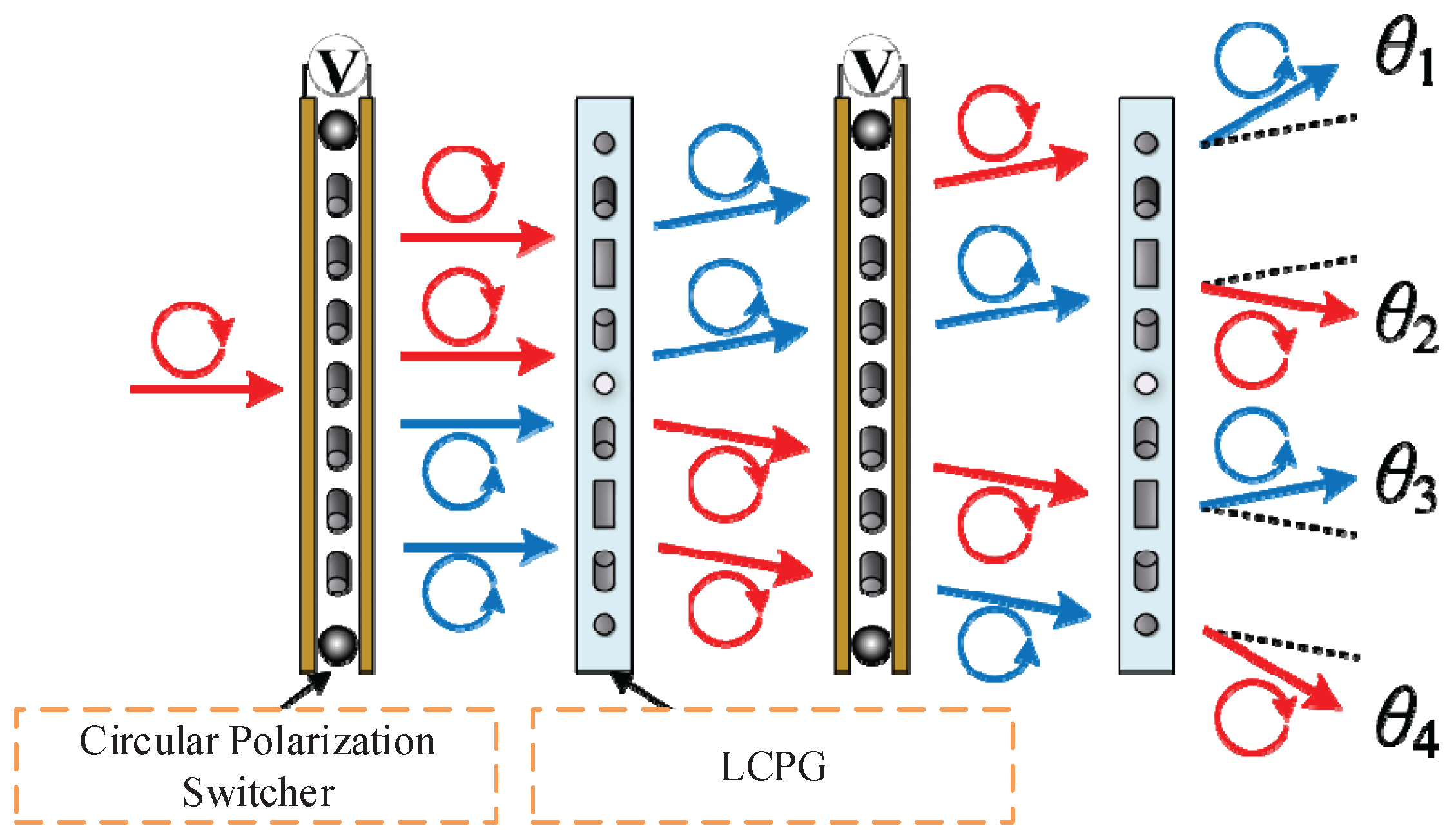
Figure 2.
Schematic diagram of the coarse-fine two-stage synchronous control system for LCOPA.

Figure 3.
Time-domain dynamic characteristics of the LCOPA during power-on.
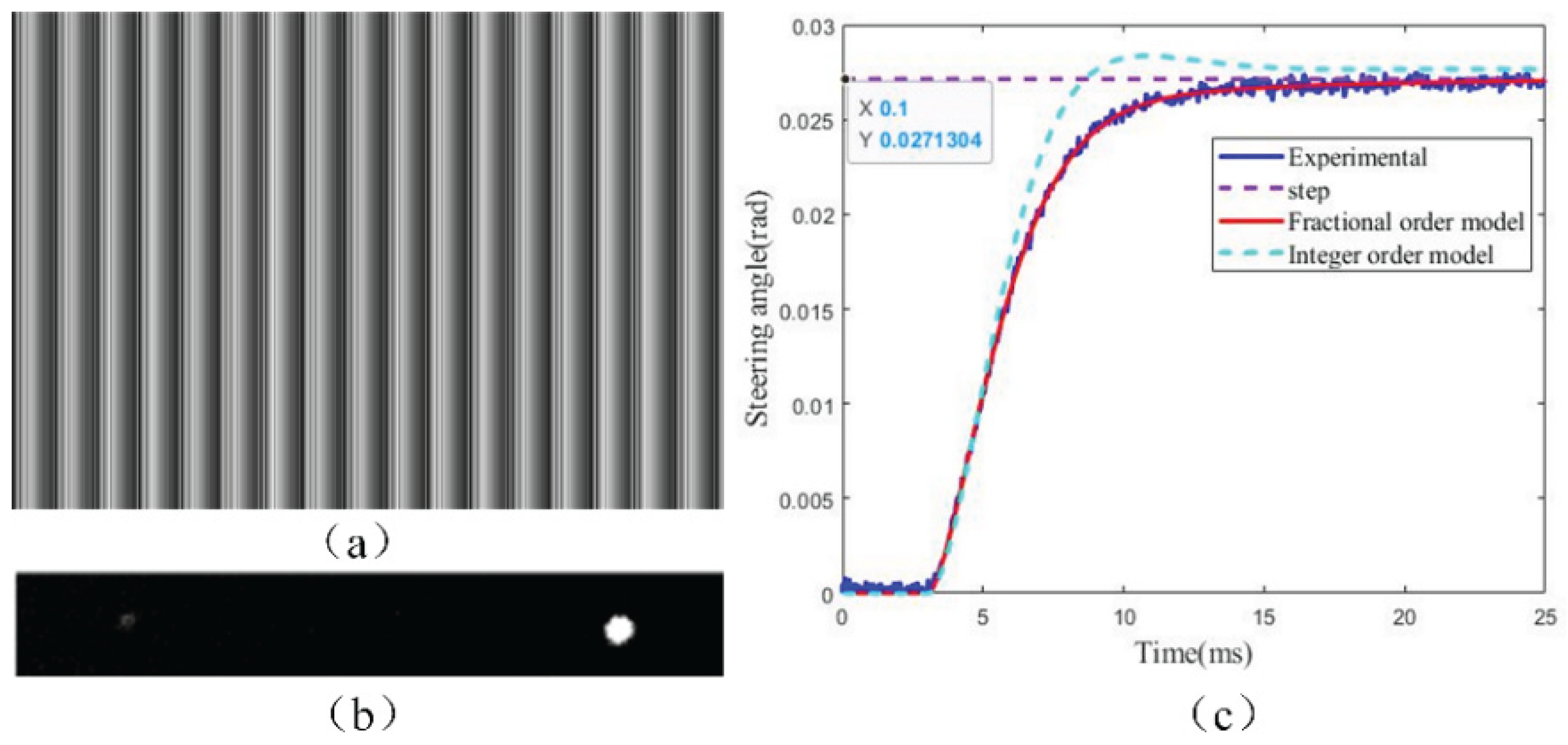
Figure 4.
Time-domain dynamic characteristics of the LCOPA during power-off.
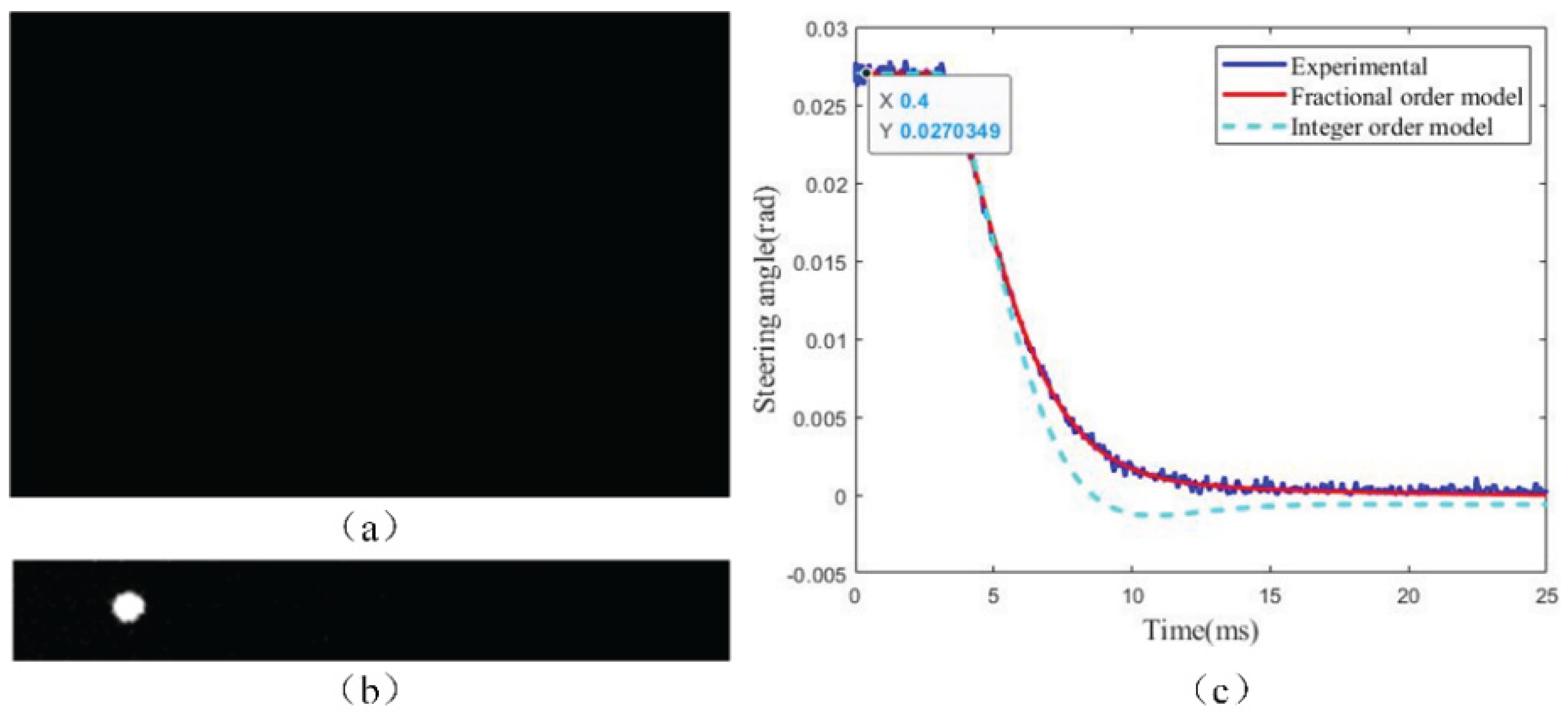
Figure 5.
Frequency-domain characteristics of integer-order and fractional-order models of the LCOPA.
Figure 5.
Frequency-domain characteristics of integer-order and fractional-order models of the LCOPA.
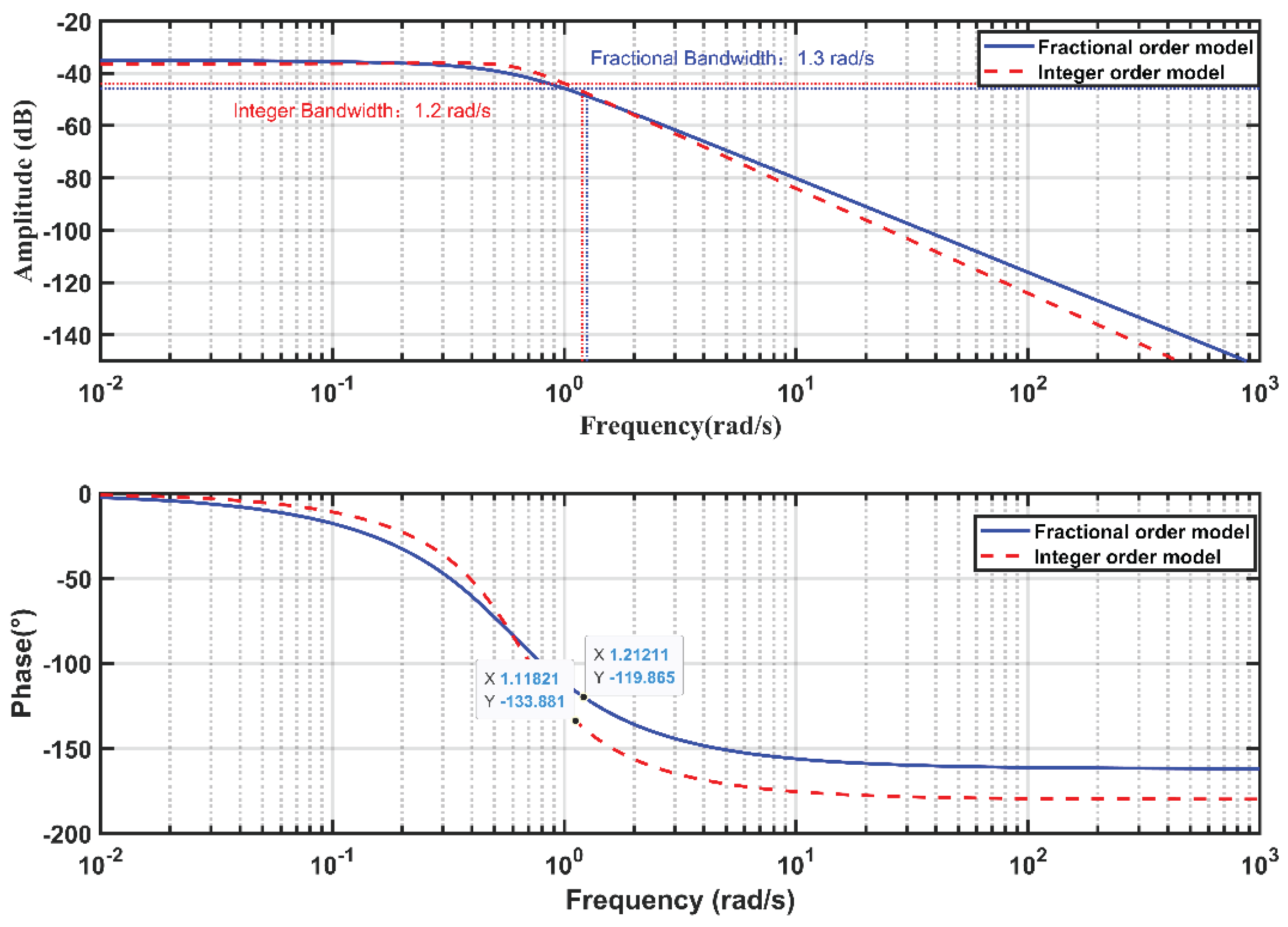
Figure 6.
Control block diagram of the fractional-order composite controller.
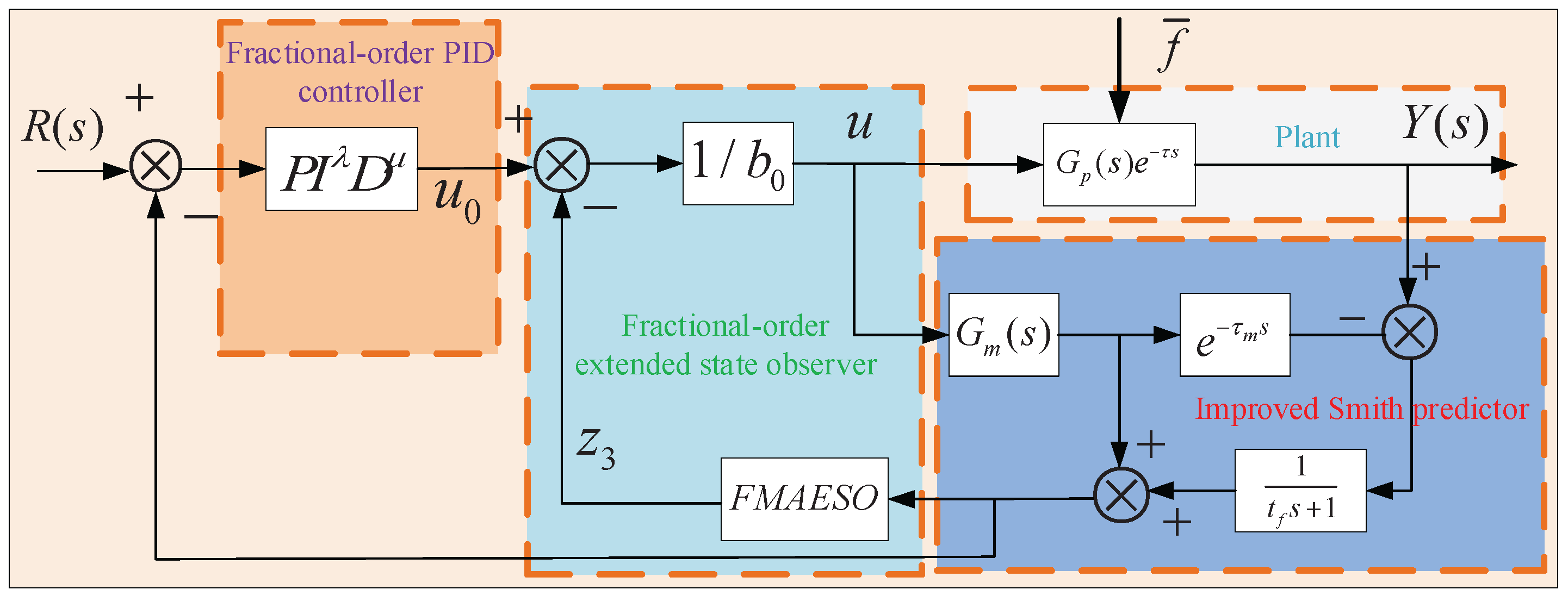
Figure 7.
Design of the Smith predictor.
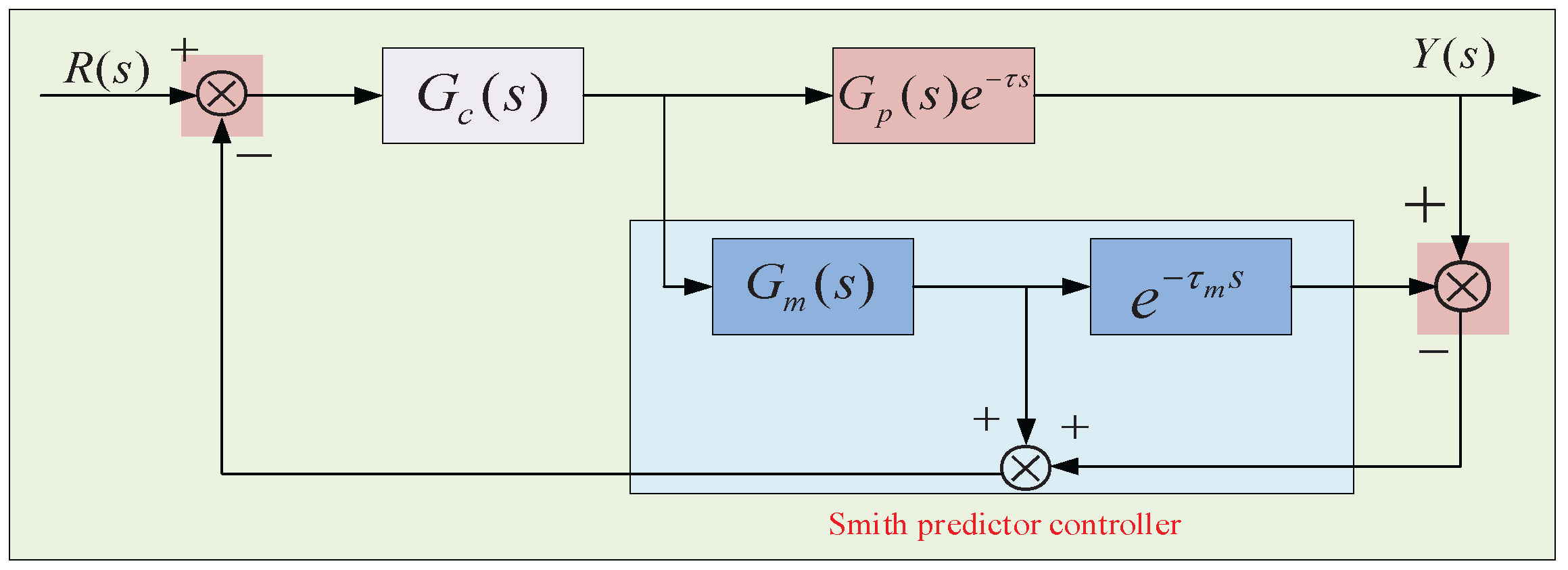
Figure 8.
Design of the improved Smith predictor.
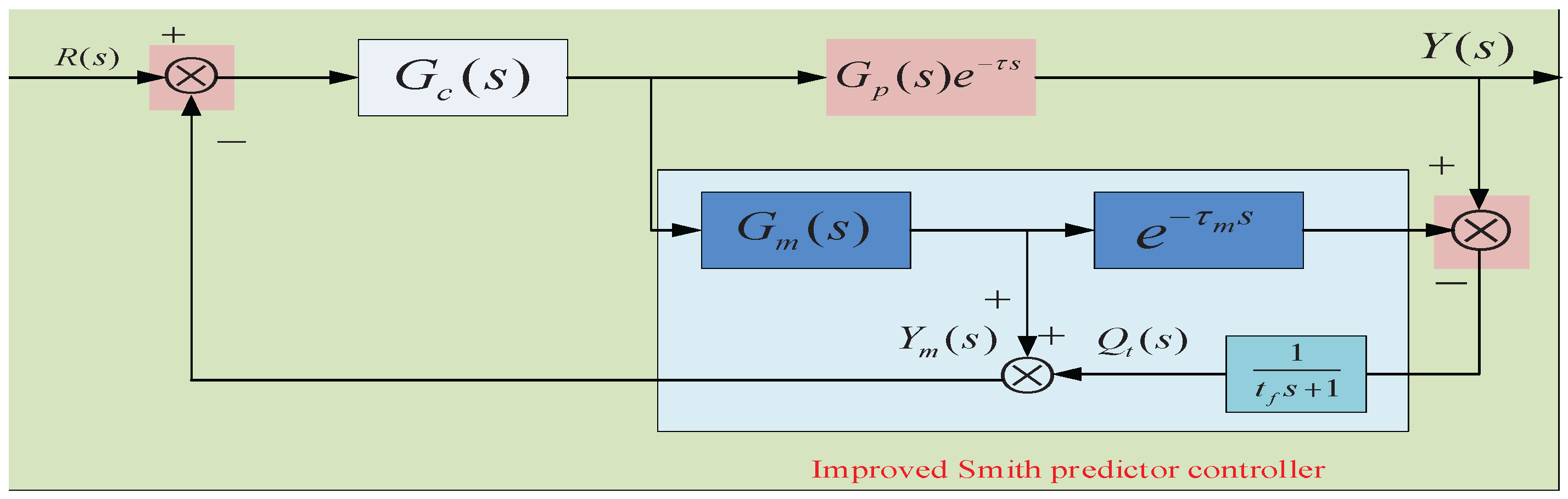
Figure 9.
Design of the extended state observer.
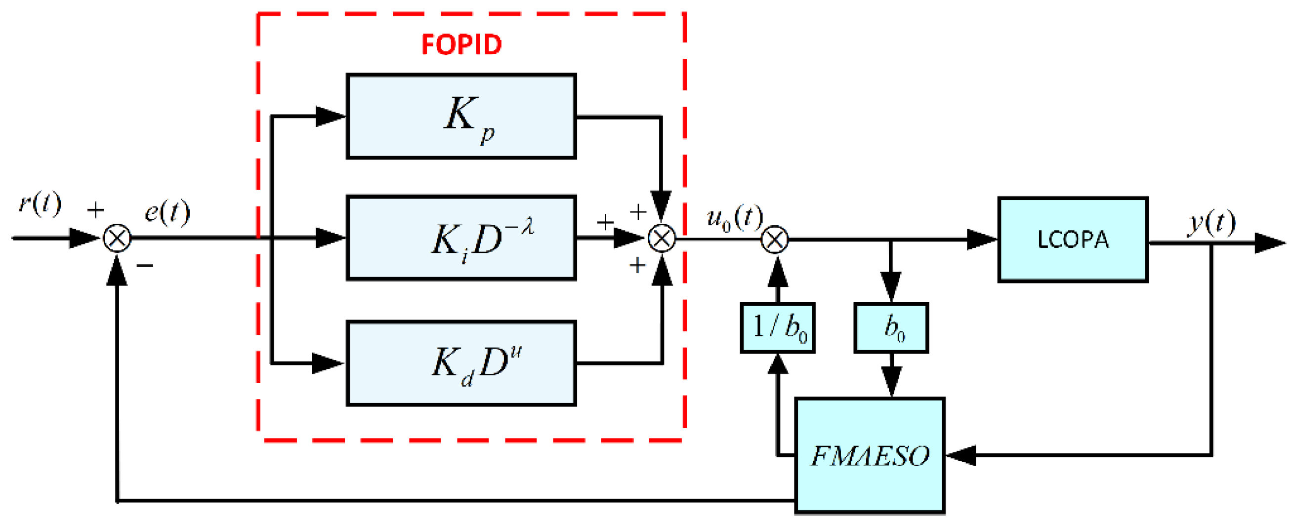
Figure 10.
Comparison of step responses and errors of different controllers: (a) Comparison of step responses of different controllers; (b) Comparison of error values of different controllers.
Figure 10.
Comparison of step responses and errors of different controllers: (a) Comparison of step responses of different controllers; (b) Comparison of error values of different controllers.
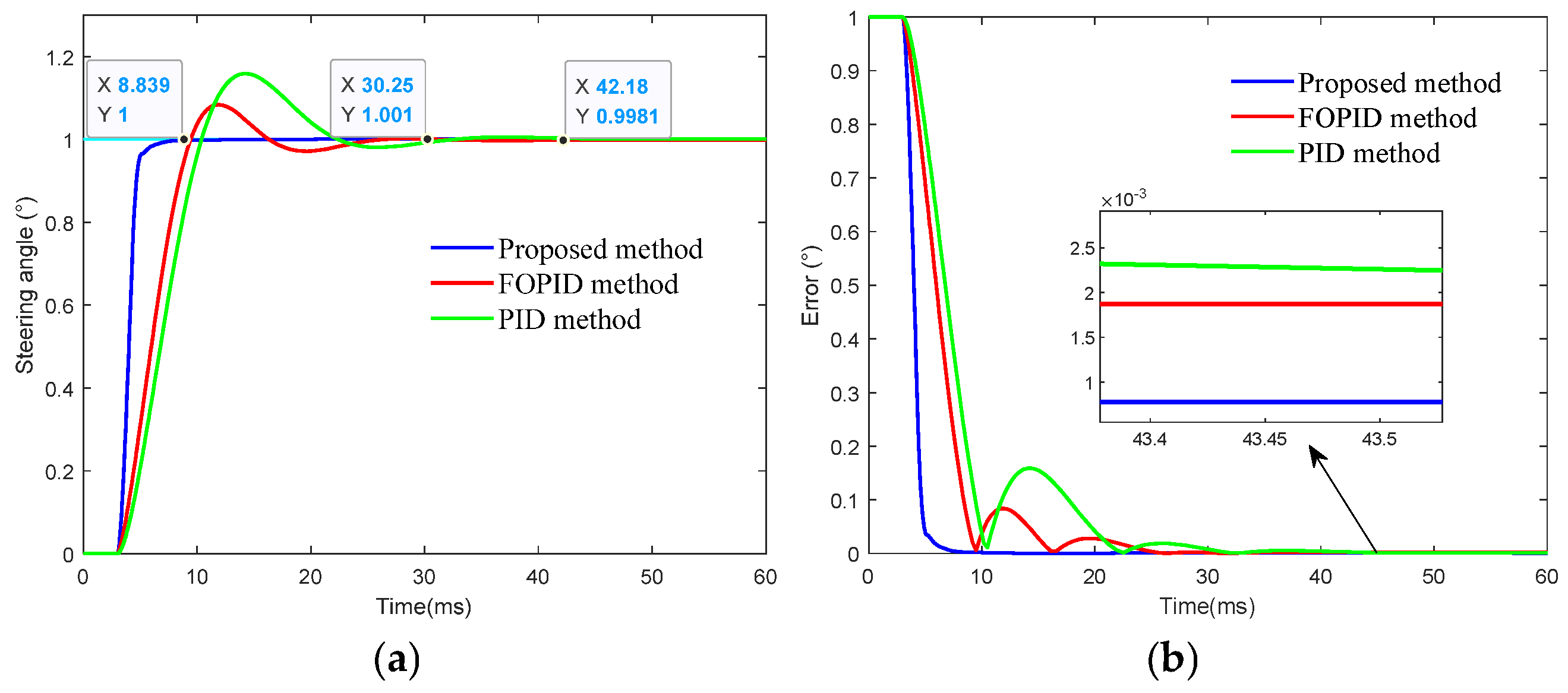
Figure 11.
Comparison of control performance of different controllers during polyline scanning of the beam: (a) Equally spaced variation of target trajectory; (b) Tracking absolute error.
Figure 11.
Comparison of control performance of different controllers during polyline scanning of the beam: (a) Equally spaced variation of target trajectory; (b) Tracking absolute error.
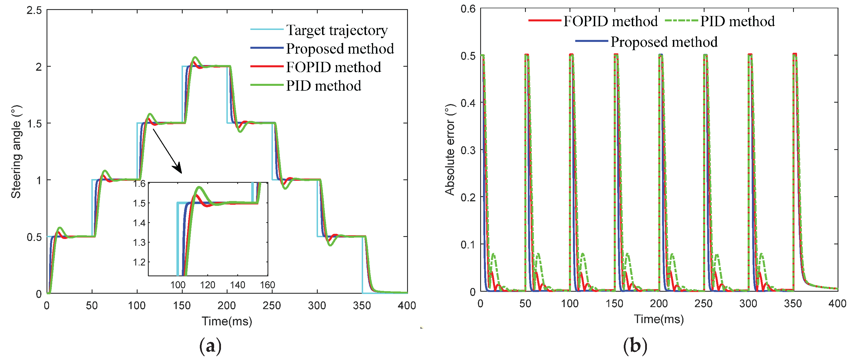
Figure 12.
Comparison of control performance of different controllers during continuous scanning of the beam: (a) Continuous variation of target trajectory; (b) Tracking absolute error.
Figure 12.
Comparison of control performance of different controllers during continuous scanning of the beam: (a) Continuous variation of target trajectory; (b) Tracking absolute error.
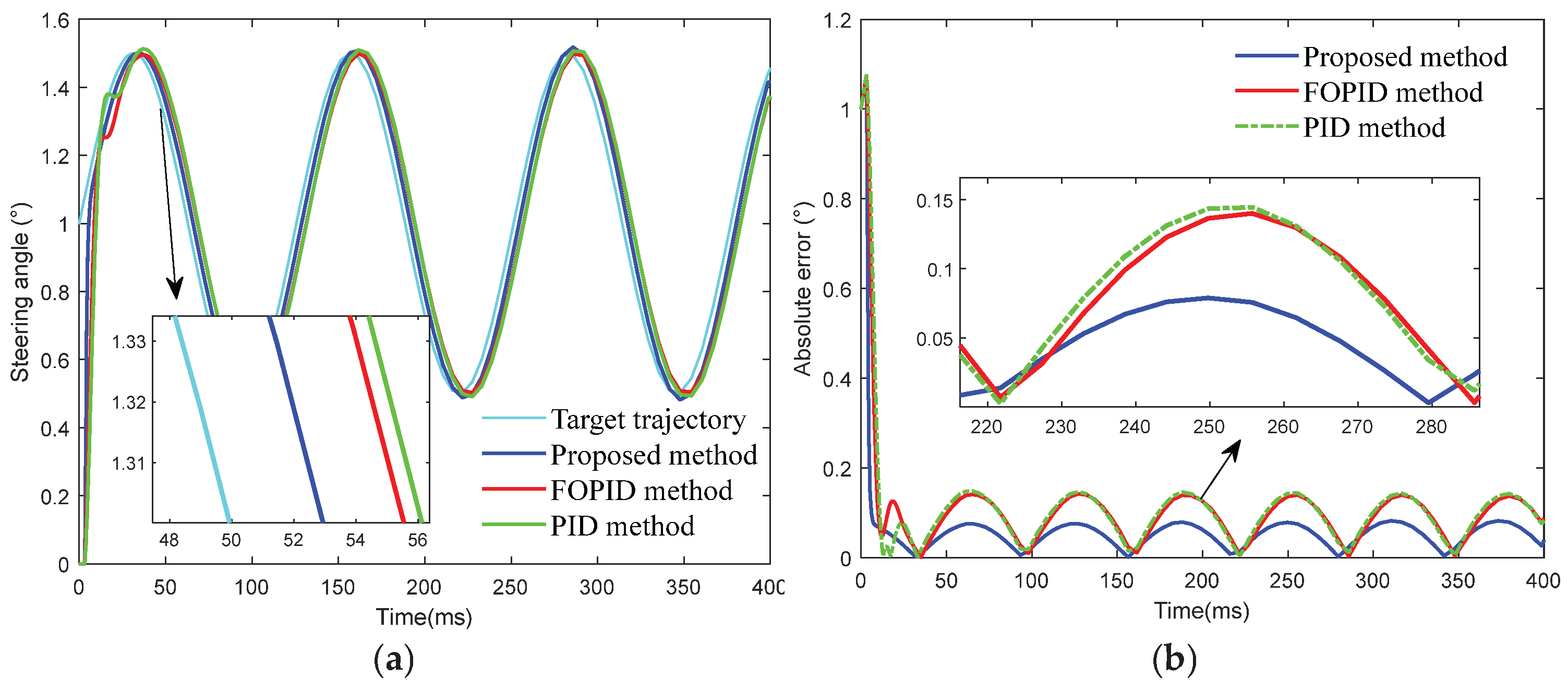
Figure 13.
Comparison of control performance of different controllers when the beam switches between fixed points: (a) Periodic variation of target trajectory; (b) Tracking absolute error.
Figure 13.
Comparison of control performance of different controllers when the beam switches between fixed points: (a) Periodic variation of target trajectory; (b) Tracking absolute error.
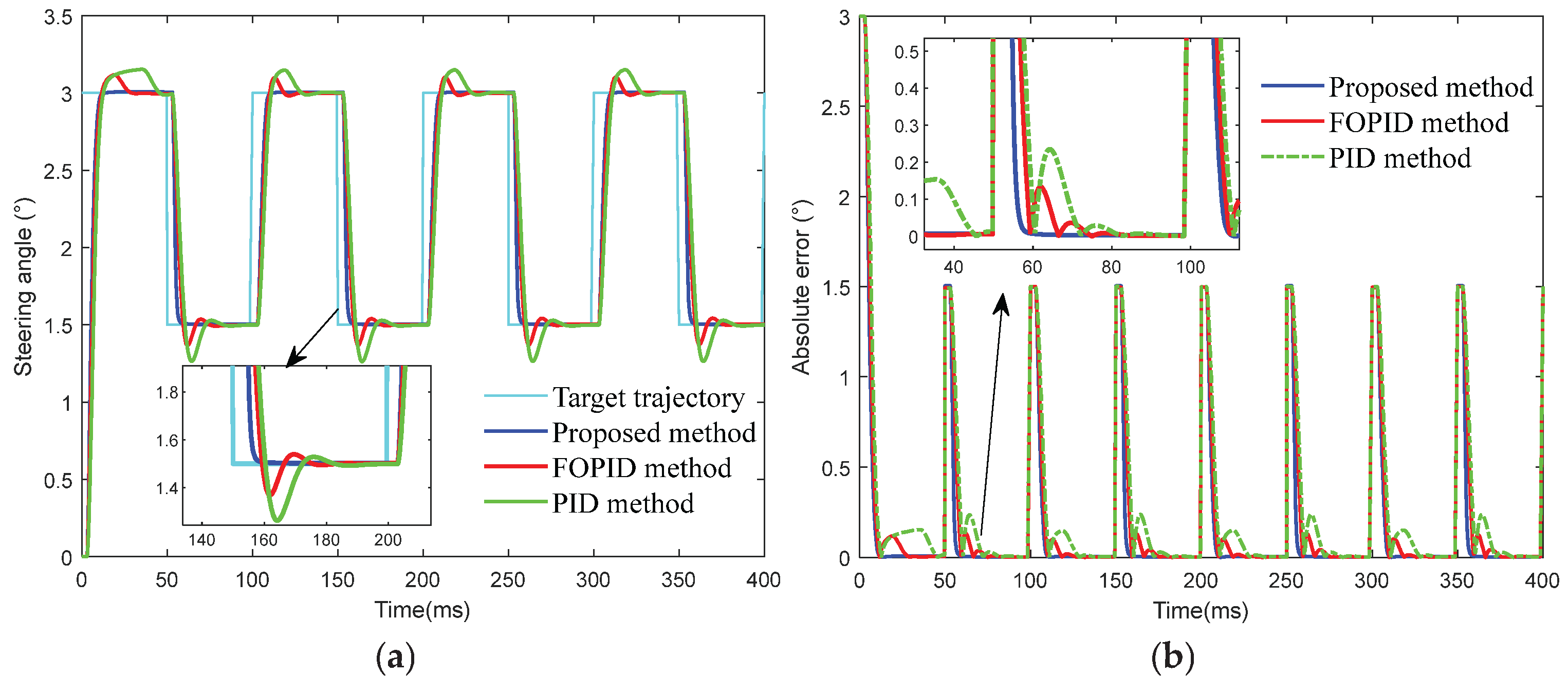
Figure 14.
Dynamic response of the system under external disturbances: (a) Step disturbance amplitude = +0.2°; (b) Step disturbance amplitude = −0.2°.
Figure 14.
Dynamic response of the system under external disturbances: (a) Step disturbance amplitude = +0.2°; (b) Step disturbance amplitude = −0.2°.
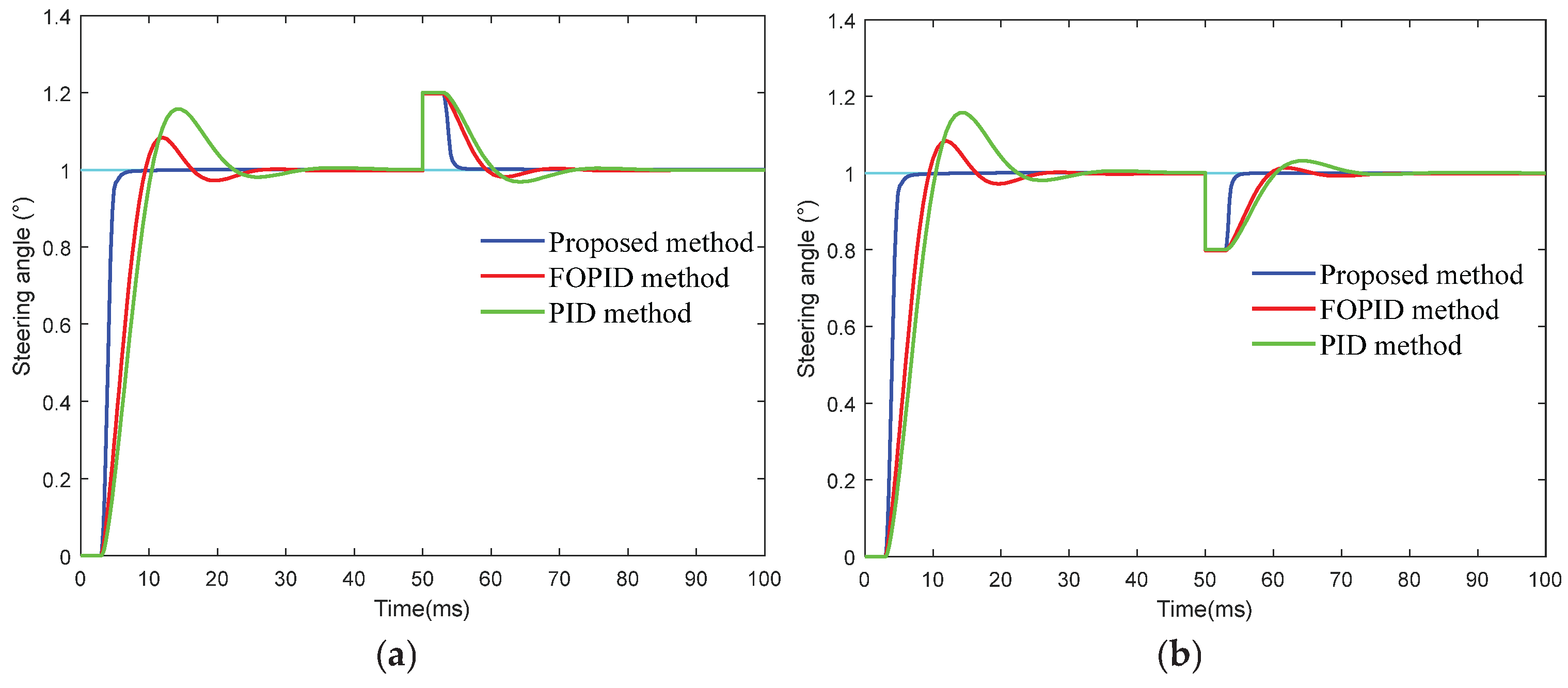
Figure 15.
System output when model parameters and Change.
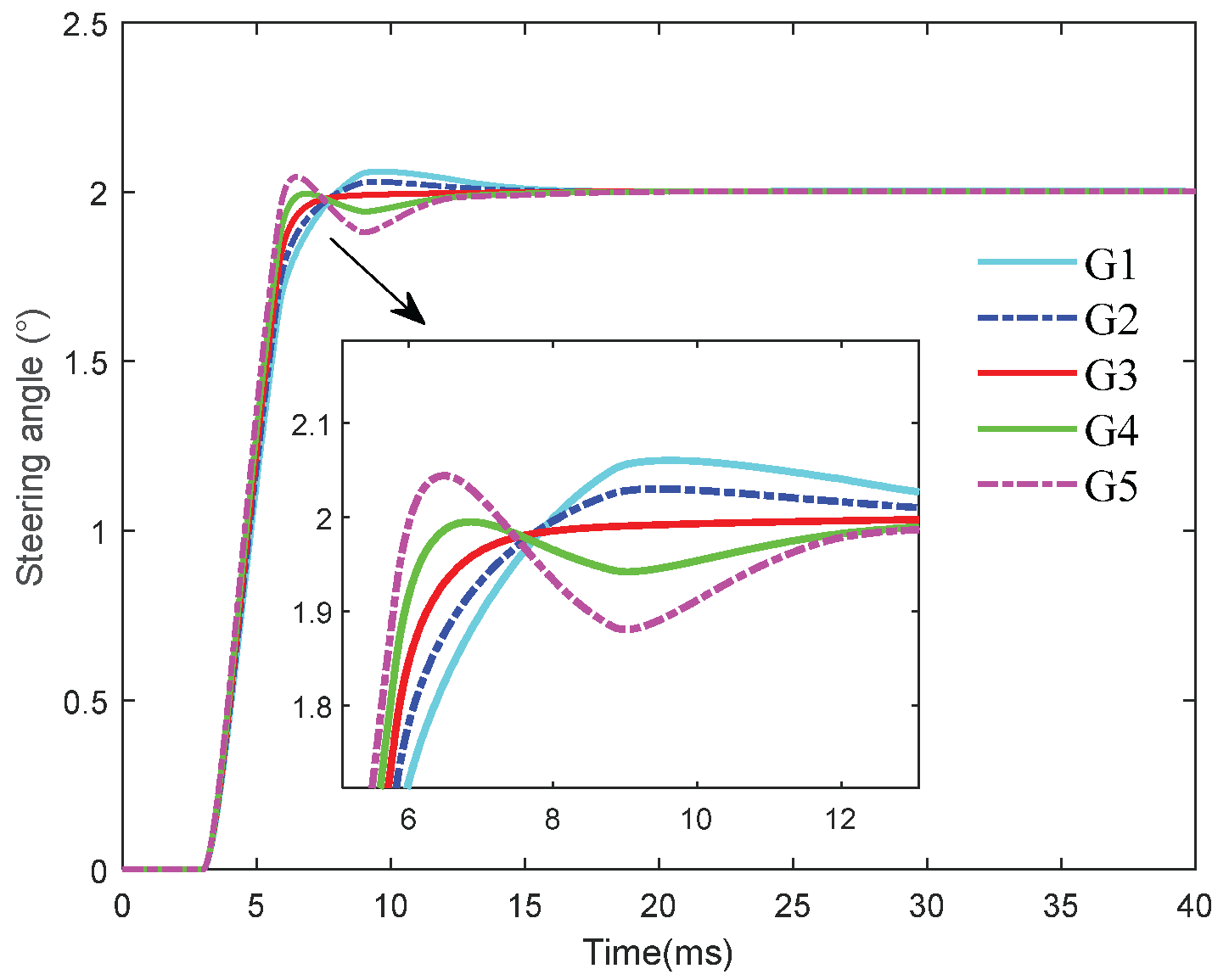
Figure 16.
System output when model order
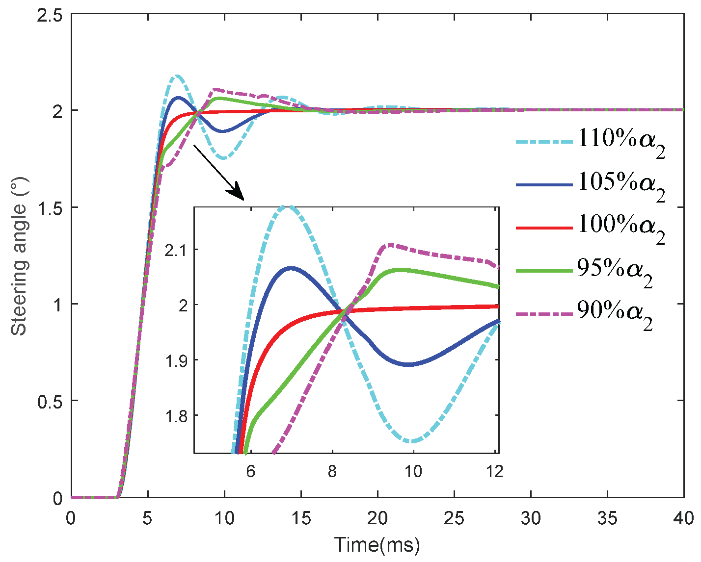
Figure 17.
System output when model order changes.
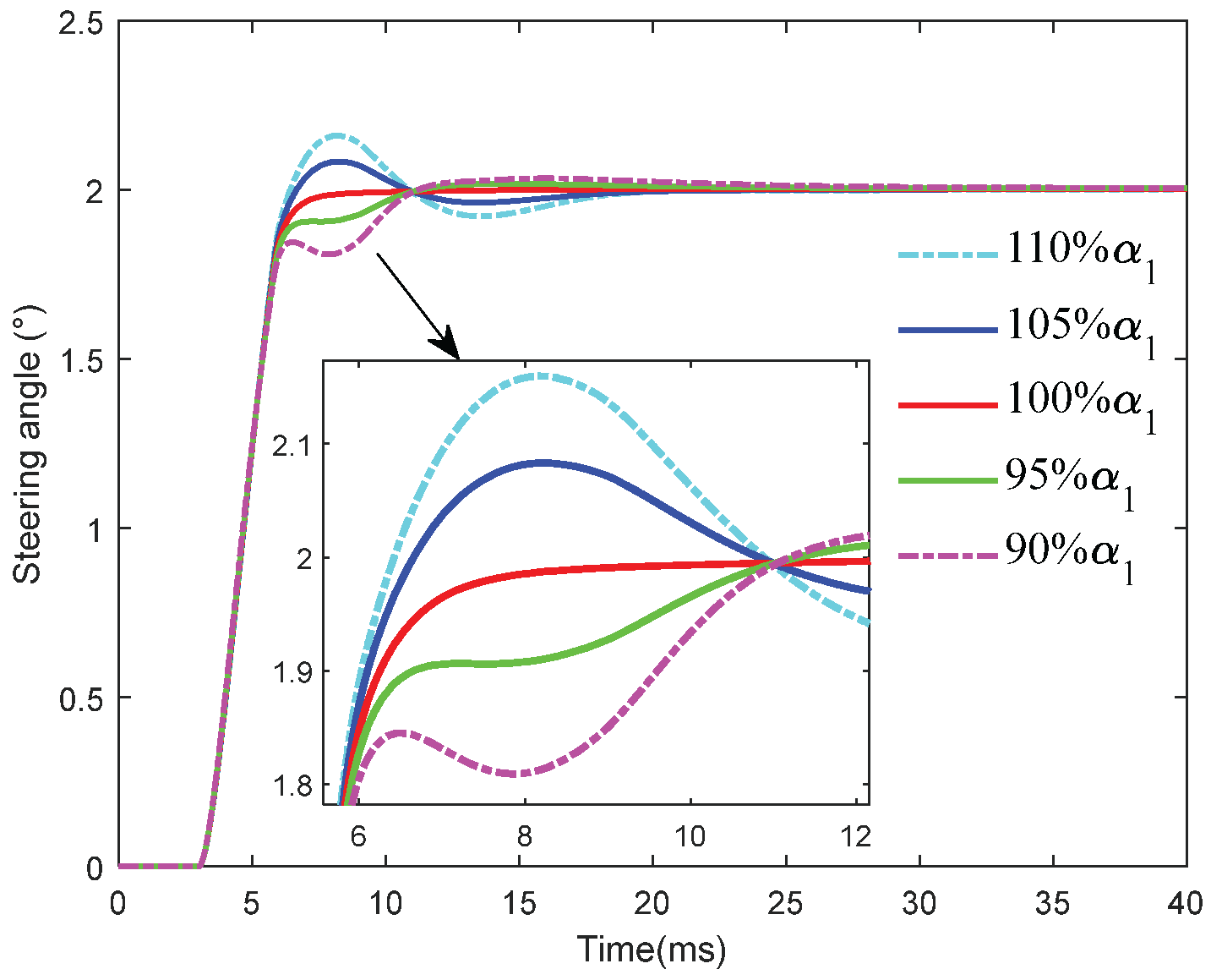
Figure 18.
Dynamic response of the system when controller gain changes.
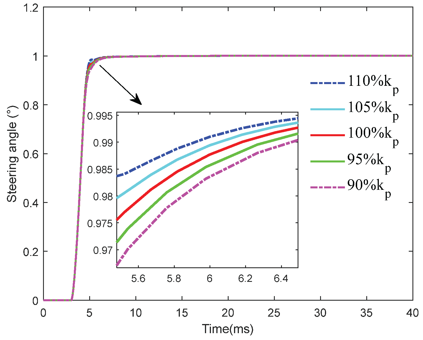
Figure 19.
System response when integral order
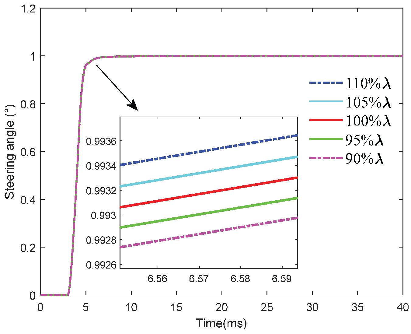
Figure 20.
System response when differential order
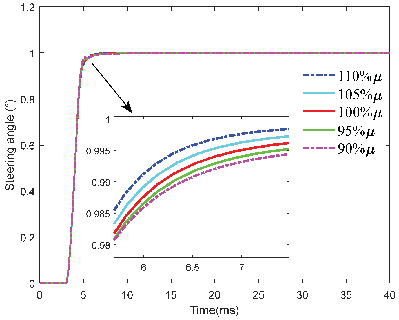
Figure 21.
Experimental platform of the coarse-fine two-stage synchronous control system for LCOPA.
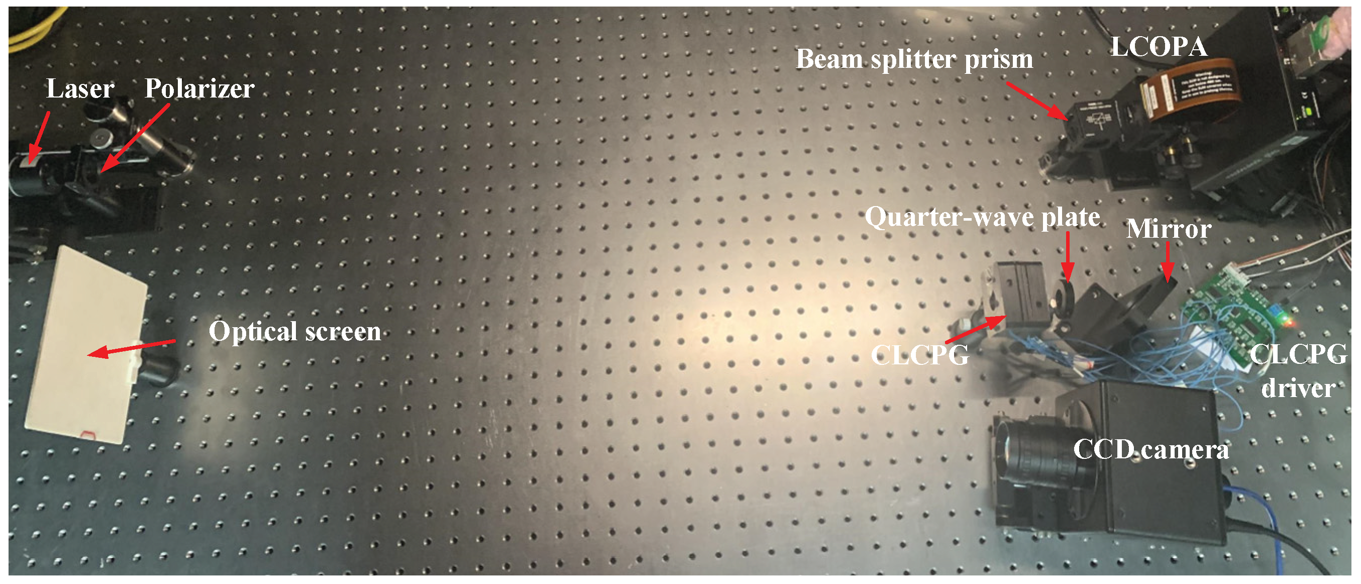
Figure 22.
Comparison results of system response speed: (a) Response speed comparison; (b) LabVIEW output results.
Figure 22.
Comparison results of system response speed: (a) Response speed comparison; (b) LabVIEW output results.
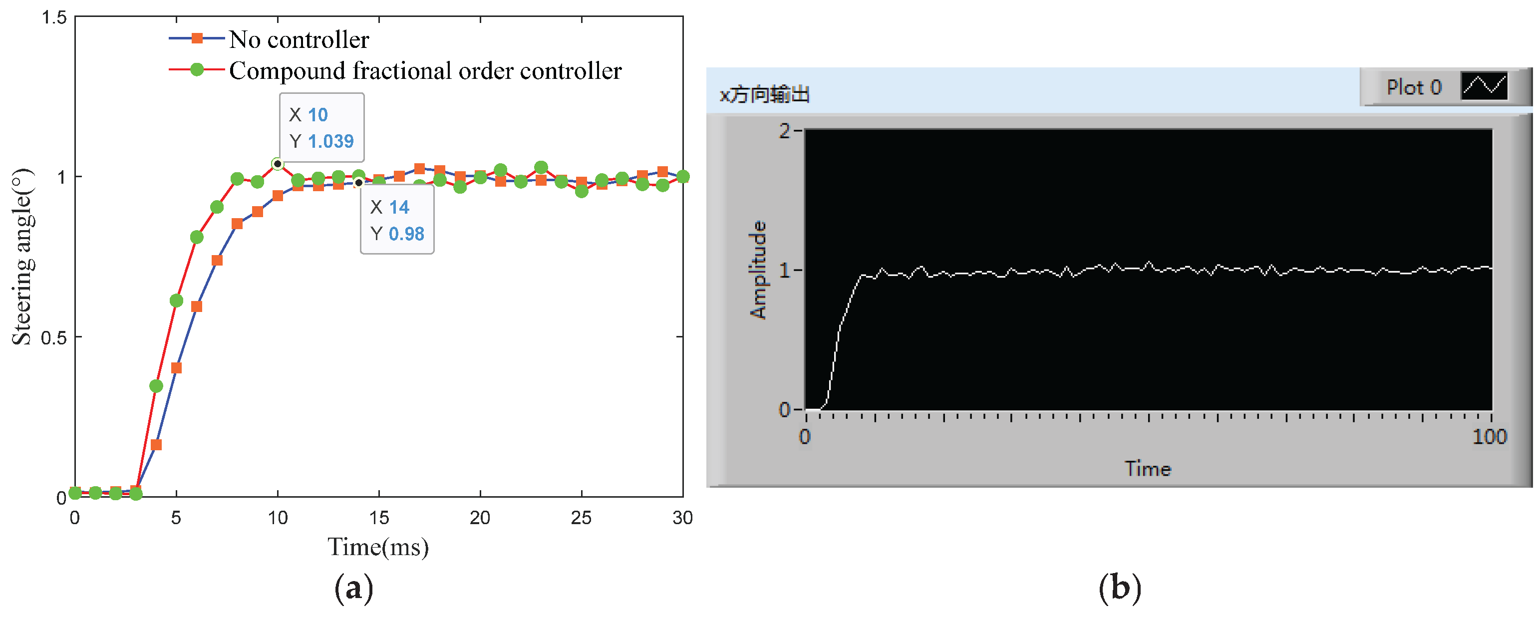
Figure 23.
Beam pointing error without the operation of the fine control system.
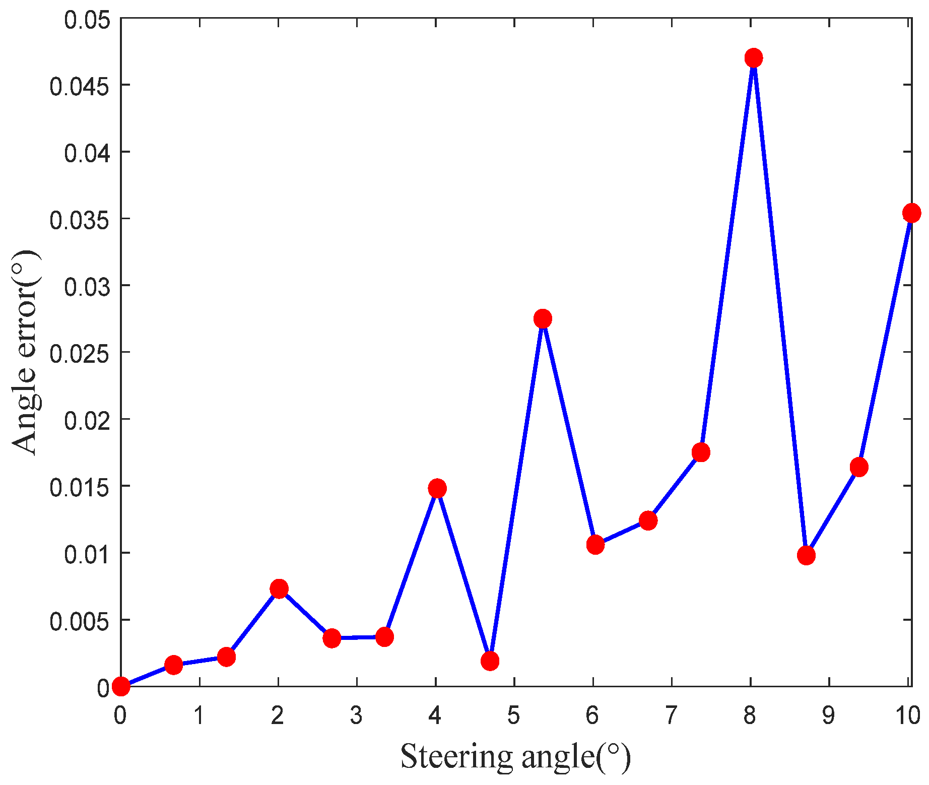
Figure 24.
Comparison of beam pointing accuracy before and after compensation by the fine control system.
Figure 24.
Comparison of beam pointing accuracy before and after compensation by the fine control system.
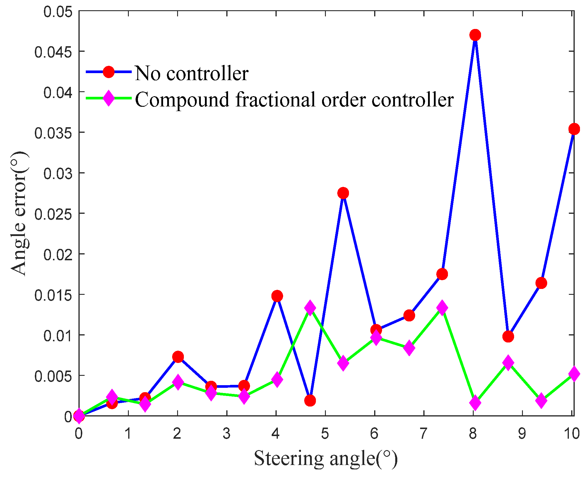
Figure 25.
Disturbance rejection performance test results of the coarse-fine two-stage synchronous control system for LCOPA: (a) Disturbance amplitude = −1°; (b) Disturbance amplitude = +1°.
Figure 25.
Disturbance rejection performance test results of the coarse-fine two-stage synchronous control system for LCOPA: (a) Disturbance amplitude = −1°; (b) Disturbance amplitude = +1°.
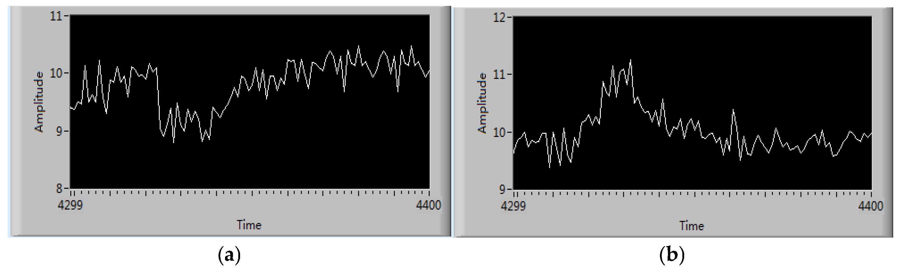
Table 1.
Comparison of control performance of different controllers.
| Response Speed (ms) | Overshoot (%) | ITAE Criterion | |
|---|---|---|---|
| Compound Fractional-Order Controller | 8.84 | 0.1 | 330.85 |
| FOPID Controller | 30.25 | 8.3 | 498.31 |
| PID Controller | 42.18 | 15.9 | 548.13 |
Table 3.
Beam pointing accuracy without the operation of the fine control system.
| Beam Spot Centroid Position | Actual Deflection Angle | Theoretical Deflection Angle | Angle Error |
|---|---|---|---|
| 0 | 0° | 0° | 0.0000 |
| 73.508 | 0.6716° | 0.67° | -0.0016 |
| 146.446 | 1.3378° | 1.34° | 0.0022 |
| 220.880 | 2.0173° | 2.01° | -0.0073 |
| 293.139 | 2.6764° | 2.68° | 0.0036 |
| 366.662 | 3.3463° | 3.35° | 0.0037 |
| 442.331 | 4.0348° | 4.02° | -0.0148 |
| 514.669 | 4.6919° | 4.69° | -0.0019 |
| 585.321 | 5.3325° | 5.36° | 0.0275 |
| 661.244 | 6.0194° | 6.03° | 0.0106 |
| 738.036 | 6.7124° | 6.70° | -0.0124 |
| 813.056 | 7.3875° | 7.37° | -0.0175 |
| 880.535 | 7.9930° | 8.04° | 0.0470 |
| 961.799 | 8.7198° | 8.71° | -0.0098 |
| 1037.734 | 9.3964° | 9.38° | -0.0164 |
| 1115.367 | 10.0854° | 10.05° | -0.0354 |
Table 4.
Pointing accuracy of the beam control system after compensation.
| Beam Spot Centroid Position | Actual Deflection Angle | Theoretical Deflection Angle | Angle Error |
|---|---|---|---|
| 0 | 0° | 0° | 0.0000 |
| 73.585 | 0.6723° | 0.67° | -0.0023 |
| 146.840 | 1.3414° | 1.34° | -0.0014 |
| 220.529 | 2.0141° | 2.01° | -0.0041 |
| 293.841 | 2.6828° | 2.68° | -0.0028 |
| 366.794 | 3.3475° | 3.35° | 0.0025 |
| 441.188 | 4.0244° | 4.02° | -0.0044 |
| 512.994 | 4.6767° | 4.69° | 0.0133 |
| 587.628 | 5.3534° | 5.36° | 0.0066 |
| 661.344 | 6.0203° | 6.03° | 0.0097 |
| 737.593 | 6.7084° | 6.70° | -0.0084 |
| 812.588 | 7.3833° | 7.37° | -0.0133 |
| 885.591 | 8.0383° | 8.04° | 0.0017 |
| 961.429 | 8.7165° | 8.71° | -0.0065 |
| 1036.103 | 9.3819° | 9.38° | -0.0019 |
| 1111.957 | 10.0552° | 10.05 | -0.0052 |
Disclaimer/Publisher’s Note: The statements, opinions and data contained in all publications are solely those of the individual author(s) and contributor(s) and not of MDPI and/or the editor(s). MDPI and/or the editor(s) disclaim responsibility for any injury to people or property resulting from any ideas, methods, instructions or products referred to in the content. |
© 2026 by the authors. Licensee MDPI, Basel, Switzerland. This article is an open access article distributed under the terms and conditions of the Creative Commons Attribution (CC BY) license (http://creativecommons.org/licenses/by/4.0/).
Copyright: This open access article is published under a Creative Commons CC BY 4.0 license, which permit the free download, distribution, and reuse, provided that the author and preprint are cited in any reuse.


