Submitted:
27 January 2026
Posted:
29 January 2026
You are already at the latest version
Abstract
Counter and concurrent flow in channels separated by membrane were studied to simulate the mass transfer through the membranes in many experimental and theoretical published research, where limited of them use the computational fluid dynamics (CFD). The current study aims to numerically simulate and physically describe the mass transfer in the counter current flow by solving Navier–Stokes (N-S) equations in the channel and membrane holes (vertical channels), while most of the previous studies, the channel flow is simulated by using N-S equations and ultra-filtration flow (membrane holes-vertical channel) is simulated by using Darcy’s Law. Consequently, the current study was implemented by using CFD to achieve several significances: avoiding the experimental tests execution, reducing the effort of module design for expensive and time-consuming, and easy observing of the variations in pressure, horizontal and vertical velocity for the model. Two-dimensional CFD Methods directly simulated the flow in channels and membrane holes to solve the Navier-Stokes (N-S) equations in each point in the whole domain where the velocity (horizontal and vertical) and pressure are calculated. In the current study it was found that the pressure decreases from inlet to the outlet of the upper and lower channel, the horizontal velocity decreases from the inlet to middle of the upper and lower channel length and increases to the outlet of the upper and lower channel, and the vertical velocity decreases from the inlet to the middle of the upper and lower channel length and increases to the outlet of the upper and lower channel. The results perfectly explored and displayed the flow distribution patterns inside channels and described the ultra-filtration profiles along the surface and in the holes of the porous membrane which is like the hemodialysis process.
Keywords:
membrane
; CFD
; N-S equations
; Darcy’s law
; Poiseuille flow
; counter current flow
1. Introduction
The flow in the channels was developed over several decades. Several research were performed to study the flow in the channels with different assumption and boundary conditions. Babu, V. (2022) and reported the analytical solution of Poiseuille flows:
P = [12*μ * u mean * L] / (h2) (1)
Where:
P = pressure at the inlet of the channel.
u mean = Mean horizontal velocity at the inlet of channel.
μ = Dynamic Viscosity (kg /m.s)
L = Length of the channel.
h = Height of the channel.
However, flow between two porous parallel plates is reported by few researchers. The Navier-Stokes equations have been solved to obtain a complete description of the fluid flow of two-dimensional incompressible steady-state laminar flow in a channel having a rectangular cross section. One side of the cross section, representing the distance between the porous walls, is much smaller than the other with two equally porous walls which leads to detailed expressions for the dependence of the velocity components and the pressure on position coordinates, channel dimensions, and fluid properties (Berman A. S, 1953). Computer simulation was used to model the flow field in crossflow membrane filtration in a porous tube and shell system. Porous (permeable) wall flow is represented by the Darcy equation which relates the pressure gradients within a flow stream to the flow rates through the permeable walls of the flow domain. The feed stream is modelled by the Navier—Stokes equations to represent viscous laminar Newtonian flow. Nassehi, (1998) developed a fluid dynamic model for crossflow filtration which is robust, accurate and cost-effective finite-element simulation scheme to link the Navier—Stokes and the Darcy equations in a solution. Damak et al, (2004) solved a fluid dynamic model of a crossflow filtration tubular membrane by numerical simulations using a finite difference scheme that were performed for laminar fluid flow in a porous tube with variable wall suction. The flow rates through the permeable wall were modeled by Darcy’s law that relates it to the pressure gradient within a flow stream. The feed stream in the tube, which flows mainly tangentially to the porous wall, is modelled by the Navier-Stokes equations. The solution depends on both the Reynolds axial and filtration number. Babu, V. (2022) reported the analytical solution of the Poiseuille flows between two porous parallel plates for two – dimensional incompressible fluid flow. There is a crossflow (vertical velocity) along the y-direction due to the walls being porous. The analytical solution was found by applying the continuity equation and Navier-Stokes equations with specific assumptions and boundary conditions. The solution depends on the cross-stream Reynolds number. During the last decades, the flow in the channels and membranes has been studied by several researchers but Computational fluid dynamics (CFD) were used in limited research to simulate the fluid flow. Karode, (2001) reported an analytical solution for the pressure drop in a rectangular slit with constant wall velocity being proportional to the trans-membrane pressure difference (constant wall permeability) and tube with porous (permeable) walls for the constant wall permeability. Numerical CFD simulation for constant wall permeability is reported for comparison. The pressure drops in crossflow membrane modules are a function of wall permeability, channel dimension, axial position and fluid properties. Pak et al., (2008) numerically simulated the laminar fluid flow in porous tubes (crossflow filtration tubular membrane) using the computational fluid dynamics (CFD) techniques. A two-dimensional numerical solution of the coupled Navier–Stokes, Darcy’s law and mass transfer equation has been developed using control volume based finite difference method. They studied the effects of geometrical dimension, required membrane surface area, Reynolds number and fouling on the performance of membrane. Khor et al., (2009) modeled the crossflow membrane filtration through the relationship between hydrodynamics and the transfer of the flows across the membrane. From the model, some connecting variables are identified and established in this modeling work. By attaining these connections, optimization of membrane filtration can be achieved by adjusting the operating parameters. The FLUENT simulated model is in good agreement with experimental results. However, Giorges et al., (2015) simulated the actual micro-pore flow and the porous medium flow (Darcy flow) for various pressure and pore sizes (porosity and permeability) by using two-dimensional CFD models to solve Navier-Stokes equations in all regions including pores and to find pore flow average outlet velocity by using porous medium characteristics.
In membrane filtration processes where a combined free and porous flow occurs, Navier-Stokes equations used to model free flows, while Darcy’s law used to model flows in porous media with small porosity. A combination of free flow and flow through porous media occurs and the continuity of flow field regime across the interface between laminar flow and porous region can be modeled by coupling Darcy’s law and the Navier-Stokes equations.
Separation by membranes plays an important role in the processing industries and in the medical sector, such as hemodialysis. There are many models developed to simulate mass transfer in hemodialysis. Counter current flow is modelled using N-S equations while membrane flow is simulated using the Darcy’s law and Kedem - Katchalsky (K-K) equations. Nassehi (1998), Eloot et al. (2002), Liao et al. (2003, 2004, 2005), Ding et al. (2004, 2015), and Cancilla et al. (2022) used different computer models with finite elements for simulation. While Abaci et al. (2010) used Stokes–Einstein’s equation for mass and momentum transfer. However, Donato et al. (2017) used Darcy’s law -Brinkman equations for flow across the membrane. Fiber in dialyzer is modeled to calculate mass transfer in the channels and membrane.
Computational fluid dynamics (CFD) has become an essential tool for analyzing complex transport phenomena in membrane-based systems, which are important for a wide range of applications from water purification to biomedical devices like hemodialysis (Stamatialis et al., 2008; Ronco et al., 2018). In processes such as hemodialysis, the counter-current flow configuration- where two fluid streams move in opposite directions on either side of a semi-permeable membrane- is widely employed due to its potential for maximizing the concentration gradient and enhancing mass transfer efficiency compared to co-current flow (Baldwin et al., 2016; Kim et al., 2013).
The fundamental function of these systems relies on the transport of solutes (e.g., urea in blood) across the membrane, driven by diffusion (concentration gradient) and convection (pressure gradient). Accurately modeling this transport is complex, as it involves coupled flow phenomena in the open channels and through the membrane's holes. A common approach in the literature has been to combine the Navier-Stokes equations for channel flow with simplified models like Darcy's law or the Kedem-Katchalsky equations for flow through the membrane (Eloot et al., 2002; Nassehi, 1998; Abaci et al., 2010). While this hybrid approach is practical, it depends on empirically determined membrane properties and may not fully resolve the detailed flow physics within the membrane's holes themselves.
Recent studies have advanced the modeling of hollow fiber dialyzers, focusing on module-scale performance and mass transfer (Cancilla et al., 2022; Donato et al., 2017; Zhuang et al., 2017). However, a clear gap exists in the high-fidelity, pore-scale resolution of flow within the membrane. Many models treat the membrane as a continuum, neglecting the specific hydrodynamics inside the pores, which can critically influence phenomena like back-filtration and overall separation efficiency (Lu et al., 2010). Directly solving the Navier-Stokes equations throughout the entire domain, including the membrane holes, presents a computationally intensive but more physically comprehensive alternative. This approach eliminates the need for semi-empirical membrane models and can provide deeper insight into local velocity and pressure fields that govern mass transfer.
The hollow fiber dialyzer is used in the therapy of hemodialysis. The hollow fiber dialyzer was examined by several authors. Labicki et al. (1995), Legallais et al. (2000), Ding et al. (2004), Liao et al. (2005), Lu et al. (2010), Kim et al. (2013), Cancilla et al. (2021, 2022), Donato et al. (2017), Elahi et al. (2023) studied the hollow fiber dialyzers (membrane) which are the main parts of the hemodialysis device with 15-25 cm in length, 200 µm in inner diameter, and 8000-16000 in number. While Abaci et al. (2010) used membrane with 8 nm in pore size. Lu et al. (2010) studied membrane with 40-80 nm in pore size and channel velocity 1.67-2.78 mm/s. They disclosed an existent Nano-scale reverse osmosis problem due to two opposite running confined flows (counter current flow). Because of this problem, they recommended using two flows in the same direction (concurrent flow) instead of counter current flow. However, Baldwin et al. (2016) studied blood flow in the lower channel and fluid flow (dialysate) in the upper channel in countercurrent and they found that countercurrent 20% increase in removal than concurrent. Kim et al. 2013 compared transmembrane pressure and the total filtration rate between counter current and concurrent flow in channels separated by a membrane. Cancilla et al., (2022) and Ciofalo, (2023) are the only authors that used 30 µm in membrane height (thickness) and channel flow 300-500 mL/min to examine the flow in dialyzers. The reverse osmosis happens when the hydraulic trans-membrane pressure could not overcome it and result in a back-filtration especially in channel with 10 nm height. By decreasing the diameter of hollow fiber, we are increasing their numbers and consequently we are increasing contact filtration area which will improve the filtration efficiency. Predicting and optimizing the flow through these microscopic channels is key to making dialysis faster and critical for designing more efficient hemodialysis equipment (Lu et al., 2010).
The current study displayed the flow distribution patterns inside channels and described the ultra-filtration profiles along the surface and the holes of the porous membrane to explore the process of hemodialysis. It used membrane with the holes (pore size) (vertical channels) = (4µm) and (15 µm) in height. While in hemodialysis, the membrane height = 30 µm as reported by (Cancilla et al., 2022) and depends on the concentration differences (diffusion) not convection. Mulder (1992) reported that blood and dialysis solutes in hemodialysis are present on both sides of the membrane in the absence of a pressure difference. The hemodialysis separation process works with concentration difference (difference in diffusion rate and molecular size) for thickness 10-100 µm in a porous membrane.
Counter current flow in channels separated by membrane is modeled to solve the continuity and N-S partial differential equations using finite difference methods in CFD to find the velocity and pressure at any point in in the whole flow domain including channels and the membrane holes (vertical channels).
Therefore, the current study presents a detailed CFD model of counter-current flow in channels separated by a membrane, with a specific focus on resolving the flow within the membrane pores. Unlike previous works that rely on Darcy's law, the current model solves the full Navier-Stokes and continuity equations simultaneously across the entire flow domain—the channels and the membrane holes. This methodology leverages modern computational capabilities to provide a direct and detailed visualization of the flow, pressure distribution, and ultrafiltration profiles. The primary objectives are to physically describe the flow patterns that develop under counter-current conditions and to demonstrate the advantages of a full-domain CFD solution for the design and optimization of membrane contactors, ultimately saving the time and cost associated with extensive experimental prototyping.
The main objective of the current study is to numerically simulate and physically describe the counter current flow in channels separated by a membrane by solving Navier–Stokes equations in the channel and membrane holes (vertical channels) instead of solving Darcy’s Law for membrane holes which needs execution the physical experiment, consequently, this approach will save time and cost and implemented by using CFD. The current study used CFD to solve N-S equations and to find the flow parameters in the whole domain (channel and vertical channel in membrane) where CFD characterized by the following advantages.
- CFD can precisely model and visualize the flow condition with higher accuracy compared to measure with physical equipment and to avoid the execution of experimental tests which face challenges in tiny channels and membranes.
- CFD reduces the expensive and time-consuming for physical modeling and experimental tests and identifies potential problems like back flow before manufacture of costly physical modules.
- CFD helps to observe variations in pressure, horizontal and vertical velocity in computer modeling in easy way, but in real experiments, it is very difficult to observe.
2. Materials & Methods
2.1. Model Concept
Hoskins et al. (2024) fabricated membranes using direct 3D printing with dimensions 75 µm *75 µm *15 µm (height) and pores of approximately 3.73 µm in diameter and very high porosities that reached up to 60% to be used for specific applications in microfluidics.
To examine the membrane efficiency and performance, the membrane in counter current flow in channels was modeled. The model is proposed with the following dimensions and properties as shown in Figure 1.
The current study examined the model as shown in Figure 1 to produce transmembrane pressure difference to produce mass transfer flow through the membrane holes (vertical channels).
- Upper channel is15 µm in height (flow from right to left) (backward).
- Membrane height is15 µm with the membrane hole (pore size) (vertical channels) is (4 µm) and wall thickness is (1 µm)
- Lower channel is 15 µm in height (flow from left to right) (forward).
- Channels and membrane are (6-301 µm) in length
- two opposite running flows in the model with axial mean velocity (1 m/s), viscosity (3 E−4 kg/ (m s)), and Re (1/300) with channel and membrane length (6-301 µm).
- Counter current fluid was used with the same viscosities.
The two-dimensional steady-state incompressible laminar flow of a fluid in a counter current channels having rectangular cross section separated by a membrane has been studied using the solution of the continuity and N-S equations.
Why does the current study use 2-D not 3-D? Height (h) =15 µm, Length (L) = variable and Width(w) >>> Height (h), this agrees with the justification reported by (Berman A. S. (1953) and Babu, V., (2022)). The current study considered as 2-D not 3-D to simulate the case with CFD by decreasing number of grid points and the time required for the program running.
The general continuity equation for 2-D incompressible fluid flow as reported by (Selvam, R.P. 2022).
∂u/∂x + ∂v/∂y = 0
The general N-S equations for 2-D incompressible fluid flow as reported by (Selvam, R.P. 2022).
ρ (u ∂u/∂x + v ∂u/∂y) = −∂p/∂x + μ (∂2u/∂x2 + ∂2u/∂y2) + ρgx
ρ (u ∂v/∂x + v ∂v/∂y) = − ∂p/∂y + μ (∂2v/∂x2 + ∂2v/∂y2) + ρgy
Physical properties and description of the current study are represented in Table 1 and shown in Figure 1.
2.1.1. Governing Equations
In two - Dimensional flow, the governing equations are:
(I) The continuity equation for 2-D (x, y).
∂u/∂x + ∂v/∂y =0
(II) The N-S equations for 2-D (x, y).
1/ ρ (∂p/∂x) = ν (∂2u/∂x2 + ∂2u/∂y2)
1/ ρ (∂p/∂y) = ν (∂2v/∂x2 + ∂2v/∂y2)
2.1.2. Boundary Conditions
The boundary conditions are adopted as follows and shown in Figure 2.
- At the inlet, a fully developed laminar profile is considered, i.e., Poiseuille flow. At x = 0: u = u(y) v = 0, p is calculated from u
- At the exit, a fully developed profile is assumed. At x = L ∂u/∂x =0, v=0, P = 0
- At the outlet, all derivatives in the flow direction are set to zero.
- At the walls there are no momentum fluxes crossing the boundary. At y= h: ∂u/∂y = 0, ∂ v /∂y = 0 or v=0
The solution of governing equations is modeled by using CFD. CFD Simulations help to predict how changing the geometry of these microscopic channels—such as the size, shape, and distribution of membrane pores—affects these transport processes. CFD as a useful tool is used to model flow in channels and membranes. Kim et al. (2013), Zhuang et al. (2015, 2017), Cancilla et al. (2021), and Elahi et al. (2023) used CFD simulation to study flow and mass transfer for hollow fiber membrane module in devices. They modeled N-S equations for flow in channels and modeled Darcy’s law for membrane as a porous medium. The simulation links the channel flow (upper and lower channel) and membrane flow (the ultra-filtration) is difficult because the boundary conditions on the membrane surface are hardly to be assumed (Lu et al., 2010). Giorges et al. (2015) presented CFD models where micro pores modeled using N-S equations to solve the flow in all regions including the pores. Ciofalo (2023) derived the analytical solutions for the two fluids flowing in parallel or counterflow through passages separated by a permeable wall as 1-D model.
However, the model in the current study is examined using 2D steady incompressible laminar Newtonian fluid to solve continuity and Navier-Stokes equation using FDM in CFD to determine the mass transfer and calculate the pressure and horizontal and vertical velocity in the at any point in the whole model including channels and the membrane holes (vertical channels). The physical description of the channel flow and the membrane (ultra-filtration) flow is governed by the N–S equations. The velocity components and the pressure on positional coordinates, channel dimensions and fluid properties are obtained. The CFD approach as a useful tool for flow visualization is adopted here as it provides a cost-effective and accurate means to find flow characteristics within whole domain model.
Current study used in-house CFD software, which was programed by Prof Selvam, R.P., to solve N-S equations, find pressure and velocity in the whole domain (channel and membrane), and visualize with help of Tec-plot. Most of previous studies developed models to find the solutions of N-S equations, Darcy’s law, and K-K equations. The velocity and pressure in channel flow are described by N-S equations, while filtration flow is described by (K-K) equations or Darcy’s law to predict the flow through a membrane. However, Giorges et al. (2015) directly simulated the actual micro pore by using two-dimensional CFD models to solve N-S equations in all regions including the pores. But, to the best of the authors’ knowledge, the current study is the first study that used CFD to model N-S equations in the two-dimensional counter current flow in channels separated by a membrane to find the velocity and pressure in the whole domain. Poiseuille flow equation (1) was used to calculate velocity and pressure along the channel without membrane to explain the difference in results for channels with membrane which we got from CFD. The 2D domain was gridded with uniform mesh (square grid spacing 0.25 µm *0.25 µm) of (181 * 1205) in y and x directions ∼218,100 nodes for simulations (for 45µm (2 channels &membrane) *60 holes (301µm)). The CFD program was run until the steady-state solution was obtained after numbers of iteration cycles. This approach is used because it is difficult to experimentally measure the pressure and velocity distribution at different locations.
2.2. Computational Procedure
The steady state N-S equations are approximated by the finite difference procedure. Since the Reynolds number is less than 1, the convection term is not considered in the current solver. The momentum and pressure equations are solved by the Successive Over Relaxation (SOR) procedure on a non-staggered grid. Since equal grid spacing is used all around the domain, the diagonal term for U and V (Ap term) is same everywhere and hence they are used to form the pressure Poisson equation as follows:
∇. U'-∆P/Ap=0
Here U' is the velocity vector obtained by solving the momentum equations. The above equation with P = 0 at the outlet and dP/dx=0 on the wall is used to solve for P. Once P is solved to required convergence, the velocities are updated as follows:
U= U'-(dP/dx)/Ap
V=V'-(dP/dy)/Ap
The current study examined the flow in the channel as Poiseuille flow to find the pressure and horizontal velocity variation along the channel length, which are constant for horizontal velocity and decreased in constant rate for the pressure, but the case is different for a counter current membrane flow. To understand the counter current membrane flow, the current study used the CFD software program and tec-plot visualization to calculate pressure and horizontal and vertical velocity, then tec-plot is used to visualize results.
3. Results
The current study gathered the CFD results for different channels length (6 µm to 301 µm) (1-60 holes). Figure 3 shows the horizontal velocity, vertical velocity, and pressure variation at the h/2 of the upper and the lower channels for a counter current in channel length (60 holes) with visualization in Tec-plot as the output of CFD software.
where: - x = Length of channel and membrane (No. of holes) in (μm)
- y = Height of channel and membrane in (μm)
- u = Horizontal velocity in m/s
- v = Vertical velocity in m/s
- p = Pressure in Pa.
Figure 3 shows that the horizontal velocity decreases from inlet velocity(1.5m/s) to 0.194m/s (represent 13% of the maximum velocity (1.5m/s)) at L/2of the channel length and then increases to outlet velocity (1.5m/s), vertical velocity decreases (downward direction) from inlet velocity (0.148m/s) to 0 at L/2 of the channel length and then increases (upward direction) from 0 to outlet velocity (0.148m/s) and Pressure decreases from inlet pressure (1725Pa) ((represent 36 % of the maximum pressure (4816 Pa = Poiseuille pressure) to outlet pressure (0) where the pressure does not decrease in linear rate. The CFD results do not follow the Poiseuille flow pattern.
For the channels (1-60 holes = 6-301μm in length), the results of CFD show that the horizontal velocity decreases from the inlet to some intermediate distance (channel middle) and then increases back to the outlet of the channel. The decreases in the velocity are increased as the channel length increases. The vertical velocity increases as the channel length (No. of holes) increases but does not do so at a constant rate. The direction of the vertical velocity is upward from the inlet to the middle of the channel length and changes direction to the downward from the middle to the outlet of the channel length. The flow in membrane holes is due to the pressure difference. It produces a vertical velocity that creates a flow through the membrane holes. The pressure increases as the channel length (No. of holes) increases but does not do so at a constant rate. This increase is required to create a flow through the channels and membrane holes.
The pressure (PCFD) and the velocity (UCFD, VCFD) are gathered from the computer model for the channel length (1-60 Holes) as shown in Figure 4.
Where: U = maximum horizontal velocity at L/2 of the channel length and h/2 of the channel height.
P = maximum pressure on the inlet and h/2 of the channel height.
V = maximum vertical velocity at the inlet and h/2 of the channel height.
Figure 4a shows that the pressure increases as the channel length increases. Figure 4b shows that the horizontal velocity decreases as the channel length increases. Figure 4c shows that the vertical velocity increases as the channel length increases but does not do so at a constant rate, eventually plateaus. From Figure 4, the horizontal velocity (U), vertical velocity (V), and pressure (P) can be calculated for any channel length (1-60 holes) (6-301μm) at the middle of the channel for U, and at the inlet of the channel for V and P.
In the current study, counter current flow does not follow the Poiseuille flow equation because of the existence of the holes in the membranes which take part of the horizontal velocity and the pressure in form of vertical velocity to generate flow through the holes of the membrane. The transmembrane pressure from CFD results is range from (97 Pa (0.14psi) to 1725 Pa (2.5psi)) for channel length 6-301µm. It is classified as microfiltration process according to (Mulder, 1992).
Non-Dimensional Pressure and Velocity Variation
At the inlet of the channel, the pressure, horizontal velocity, and vertical velocity for the counter current flow for the channels (20,40, and 60) holes are presented and plotted in a non-dimensional form to show the effect of the existence of a membrane as shown in Table 3 and Figure 5.
Table 3 shows that the horizontal velocity decreases while the pressure increases as the length of the channel increases. For example, the horizontal velocity (UCFD) is only 68 % of the U. max inlet and the pressure (PCFD) is only 78 % of the P Analytical for channel (20 holes) while they are 13% and 36% for channel (60 holes) as previously mentioned.
Figure 5a shows that the non-dimensional pressure increases as the non-dimensional channel length increases. Figure 5b shows that the non-dimensional horizontal velocity decreases as the non-dimensional channel length increases along with the channel length (L). Figure 5c shows that the non-dimensional vertical velocity changes from inlet to outlet, which is not linear. It decreases until the middle of the channel length (L/2) (positive/downward direction). It increases and changes its direction (negative/downward direction) to the outlet of channel.
4. Comparison of CFD Numerical Solution with 1-D Analytical (Ciofalo) Solution
There are many methods to compare simulation model results. One of the methods is an analytical solution while the other one is experimental procedures. Most studies prefer the analytical solution over the experimental procedures because of the cost and time. The current study used the 1-D analytical (Ciofalo (2023)) solution to compare with the CFD numerical results. The current study modeled the counter current flow as shown in Table 1 and Figure 1. The permeability (k), Porosity, and hydraulic permeability (Lp) parameters that were used in 1-D analytical (Ciofalo (2023)) solution were calculated as shown in Table 4.
For current study, CFD model numerical results were compared with 1-D analytical (Ciofalo, 2023) model results and Poiseuille flow between two solid parallel plates. Figure 6 shows comparison of the mean horizontal velocity for the channel length (6-301 µm) between the two models. Figure 7 shows comparison of the pressure for the channel length (6-301 µm) between the models.
There are differences between the results of 1-D analytical (Ciofalo) model and the CFD model for the current study. These differences are due to the boundary conditions and assumption and due to differences in equations that are being used to solve the flow in the channel. The CFD model uses continuity and Navier-Stokes (N-S) equations for the flow in channel and membrane holes (vertical channel), while 1-D analytical (Ciofalo) model uses continuity equation for the flow in channel and Darcy’s law for flow through membrane. The 1-D analytical (Ciofalo) model results are close to the CFD model results.
The 1-D analytical (Ciofalo) model results with the permeable wall are slightly close to CFD numerical results with membrane. The CFD model results are matched with 1-D analytical (Ciofalo) model results which give the current study results much confidence.
5. Analysis and Discussion
Most of the previous studies used N-S equations to model channels flow and Darcy’s law to model trans-membrane ultra-filtration flow (membrane flow). They found that the channel pressure drops, the trans-membrane pressure, the channel velocity, and ultra-filtration velocity are nearly linear. However, the current study used N-S equations to model channels flow and trans-membrane ultra-filtration flow (membrane flow). The mass transfer through membrane holes occurs due to the pressure differences between the upper and the lower channel. The pressure is maximum at the inlet of the channels. This means that maximum pressure occurs between the inlet of the upper channel and the outlet of lower channel and vice versa between the outlet of the upper channel and the inlet of lower channel. This maximum pressure difference makes high mass transfer flux through the membrane holes (vertical channels). This is giving an explanation why the current study uses counter current not concurrent flow. From the results of current study, the existence of membrane changes the properties of the flow from Poiseuille flow between two rigid plates to flow in channels separated by a membrane.
Noda et al. (1979), Zhuang et al. (2015, 2017), and Ciofalo (2023) determined the mass transfer for counter current flow where counter current could improve the uniformity of mass flux distribution, and the flow rate decreases from the inlet to some intermediate distance and then increases back to outlet in counter current. Gostoli et al. (1980), Davenport et al. (1990), Kim et al. (2013), and Baldwin et al. (2016) determined the mass transfer for both con-current and counter current flow, where counter current flow was more efficient and is associated with a 20% increase in removal than con-current flow. In contrast, Lu, et al. (2010) recommended con-current flow instead of counter current flow.
For the current study as shown in Table 5, the membrane pore (hole) size is (4 µm) (membrane holes-vertical channels) and the height (thickness) is (15 µm).According to the IUPAC (International Union of Pure and Applied Chemistry) the pores in the membrane are 3.75 µm and are classified as macropores > 50 nm (0.05 µm) and considered as ultrafiltration process with membrane pores 2 -100 µm (porous membrane) for ∆P =1 to 5 bar (10000 Pa – 50000 Pa). The transmembrane pressure from CFD results is range from (97 Pa (0.14psi) to 1725 Pa (2.5psi)) for channel length (6-301µm). It is classified as microfiltration process according to Mulder, (1992). In hemodialysis, the membrane height = 30 µm as reported by (Cancilla et al., 2022) and Ciofalo, 2023)) and depend on the concentration differences not on the pressure differences. Mulder (1992) reported that blood and dialysis solutes in hemodialysis are present on both sides of the membrane with absence of pressure difference and works with concentration difference (difference in diffusion rate and molecular size) for porous membrane thickness 10-100 µm.
The current study found that the horizontal velocity decreases from inlet to the middle length of channel (L/2) and increases to the outlet. The pressure decreases from the inlet to the outlet. There is a vertical velocity in the channel as the result of membrane existence which is responsible for flow through the membrane hole. The increase of the trans-membrane pressure (= upper/lower channel inlet pressure – lower/upper channel outlet pressure) causes increase in the amount of ultra-filtration. At the interface between the channel and membrane surface, the current study found that the direction of vertical velocity is upward to L/2 of the channel length and change the direction to downward from L/2 to L of the channel length. This means that the flow in the membrane holes is due to vertical velocity which produces from trans-membrane pressure differences. The pressure, Horizontal and vertical velocity variations in channel aren’t linear, but the pressure inside membrane holes (vertical channels) is linear because it is small length (15 µm) and follows Poiseuille flow. The horizontal velocity decreases from the channel inlet to the L/2 of the channel and increases to the outlet. The horizontal velocity decreases as the channel length increases to the length that horizontal velocity almost zero. This phenomenon causes trouble in the microfluidics devices through back flow and stagnation.
6. Conclusion
In the current study, Counter current flow does not follow the Poiseuille flow equation because of an increase in the holes in the membrane (channel length). The holes in the membrane take part of pressure and horizontal velocity in the form of vertical velocity to create flow in the holes of membrane. The flow pattern in the current study (2-D model) can be summarized in the following
- Horizontal velocity decreases as the length of channel increases and as the height of channel and membrane decreases
- Pressure and Vertical velocity increases as the length of channel increases and as the height of channel and membrane decreases
The current study can improve the efficiency of the device and decrease the time required to treat the patient’s blood, especially the hemodialysis, if we understand counter current flow in the channel separated by a membrane. As reported by (Liao et al., 2003, Baldwin et al., 2016, and Cancilla et al. 2022) for counter-current dialysate flow, the current study suggested that using different channel height (one channel for blood and the other channel for dialysate) is more efficient. If we find the best combination of channels height, we can increase the contact time between blood and dialysate (solute) through the membrane by increasing the vertical velocity through the membrane holes (the vertical channel), then we can decrease the time for the patient under hemodialysis and then decrease the suffering and pain. The CFD model results are matched with 1-D analytical (Ciofalo) model results which give the current study results much confidence.
7. Current Study Contributions
Most of the previous studies used CFD to model channels flow by solving Navier-Stokes (N-S) equations and to model trans-membrane ultra-filtration flow (membrane flow) by solving Darcy’s law or Kedem-Katchalsky (K-K) which needs an execution of the physical experiments to find some parameters like permeability. These studies found that the channel pressure drops, the trans-membrane pressure, the channel velocity, and ultra-filtration velocity are nearly linear. To the best of the authors’ knowledge, the current study is the first study that used CFD to model the two-dimensional counter current flow in channels separated by a membrane by solving N-S equations in channels and membrane holes (vertical channels) to find the velocity and pressure at any point in the whole domain because it is difficult to experimentally measure. Consequently, this approach as reliable tool saves cost and time. Instead of manufacturing the microfluidics devices and conducting expensive and time-consuming physical experiments, it can test and optimize hundreds of different designs of these devices.
Author Contributions
Conceptualization R.P.S.; methodology, R.P.S. and A.A.; software, R.P.S.; validation, R.P.S. and A.A.; resources R.P.S.; investigation A.A.; data curation A.A.; formal analysis, R.P.S. and A.A.; writing—original draft preparation, A.A.; writing—review and editing, R.P.S. and A.A.; visualization, A.A.; supervision, R.P.S.
Funding
This study received funding from the Civil Engineering Department/ Engineering Collage/ University of Arkansas.
Data Availability Statement
The data presented in this study is available on request from the corresponding author.
Acknowledgments
This study was funded by Civil Engineering Department/ Engineering Collage/ University of Arkansas. The authors extend great thanks to The Head of Civil Engineering Department/ Professor Hale for his assistance and support.
Conflicts of Interest
The authors declare no conflict of interest. The funders had no role in the design of the study; in the collection, analyses, or interpretation of data; in the writing of the manuscript; or in the decision to publish the results.
Nomenclature
| CFD computational fluid dynamics N-S Naveir-Stokes K-K Kedem-Katchalsky P pressure (N/m2= kg/m. s 2 = Pascal) U, u horizontal velocity (m/s) V, v vertical velocity (m/s) L channel length (m) h channel height (m) D dimension (m) Re Reynolds number |
Q flow rate (m3/s) u, v, w velocity components in x, y, z direction (m/s) g x, y, z gravity components in x, y, z direction (m/s2) Greek letters µm micrometer ρ Density (Kg/m3) μ Dynamic Viscosity (kg /m.s) ν = μ/ρ Kinematic Viscosity (m2/s) |
References
- Abaci, H. E., &Altinkaya, S. A. (2010). Modeling of hemodialysis operation. Annals of biomedical engineering, 38(11), 3347–3362. [CrossRef]
- Babu, V. (2022). Fundamentals of Incompressible Fluid Flow. Springer International Publishing AG. (eBook). [CrossRef]
- Baldwin, I., Baldwin, M., Fealy, N., Neri, M., Garzotto, F., Kim, J. C., Giuliani, A., Basso, F., Nalesso, F., Brendolan, A., & Ronco, C. (2016). Con-Current versus Counter-Current Dialysate Flow during CVVHD. A Comparative Study for Creatinine and Urea Removal. Blood purification, 41(1-3), 171–176. [CrossRef]
- Berman, Abraham S. (1953). Laminar Flow in Channels with Porous Walls. JOURNAL OF APPLIED PHYSICS, 24(9).
- Cancilla, N., Gurreri, L., Marotta, G., Ciofalo, M., Cipollina, A., Tamburini, A., Micale, G. (2021). CFD prediction of shell-side flow and mass transfer in regular fiber arrays. International Journal of Heat and Mass Transfer, 168. [CrossRef]
- Cancilla, N., Gurreri, L., Marotta, G., Ciofalo, M., Cipollina, A. Tamburini, A., Micale, G. (2022). A porous media CFD model for the simulation of hemodialysis in hollow fiber membrane modules. Journal of Membrane Science,646. [CrossRef]
- Chen,X., Shen, J. (2016). Review of membranes in microfluidics. Journal of Chemical Technology & Biotechnology, 92(2), 271-282. [CrossRef]
- Ciofalo, M. (2023). Flow Through Parallel Channels Separated by a Permeable Wall. In: Thermofluid Dynamics. UNIPA Springer Series. Springer, Cham. [CrossRef]
- Davenport, A., Will, E. J., & Davison, A. M. (1990). Effect of the direction of dialysate flow on the efficiency of continuous arteriovenous haemodialysis. Blood purification, 8(6), 329–336. [CrossRef]
- Damak, Kamel, Ayadi,Abdelmoneim, Zeghmati, B. & Schmitz, Philippe. (2004). A new Navier-Stokes and Darcy's law combined model for fluid flow in crossflow filtration tubular membranes. Desalination, 161, 67-77. [CrossRef]
- Ding, W., Li, W., Sun, S., Zhou, X., Hardy, P. A., Ahmad, S., & Gao, D. (2015). Three-dimensional simulation of mass transfer in artificial kidneys. Artificial organs, 39(6), E79–E89. [CrossRef]
- Ding, Weiping & He, Liqun & Zhao, Gang & Zhang, Haifeng& Shu, Zhiquan& Gao, Dayong. (2004). Double porous media model for mass transfer of hemodialyzers. International Journal of Heat and Mass Transfer, 4849-4855. [CrossRef]
- Donato, Danilo & Boschetti de Fierro, Adriana & Zweigart, Carina & Kolb, Michael &Eloot, Sunny & Storr, Markus & Krause, Bernd & Leypoldt, Ken & Segers, Patrick. (2017). Optimization of dialyzer design to maximize solute removal with a two-dimensional transport model. Journal of Membrane Science, 541, 519-528. [CrossRef]
- Elahi, A., & Chaudhuri, S. (2023). Computational Fluid Dynamics Modeling of the Filtration of 2D Materials Using Hollow Fiber Membranes. ChemEngineering, 7(6), 108. [CrossRef]
- Eloot, S., De Wachter, D., Van Tricht, I., & Verdonck, P. (2002). Computational flow modeling in hollow-fiber dialyzers. Artificial organs, 26(7), 590–599. [CrossRef]
- Giorges, Aklilu & Pierson, John. (2015). Modeling and CFD Simulation of Membrane Flow Process. https://doi.org/10.1115/IMECE2015-53530 Gostoli, C., Gatta, A. (1980). Mass transfer in a hollow fiber dialyzer. Journal of Membrane Science, 6, 133-148. [CrossRef]
- Hoskins, J.K.; Zou, M. (2024). 3D Printing of High-Porosity Membranes with Submicron Pores for Microfluidics. Nanomanufacturing, 4, 120–137. [CrossRef]
- Kim, J. C., Cruz, D., Garzotto, F., Kaushik, M., Teixeria, C., Baldwin, M., Baldwin, I., Nalesso, F., Kim, J. H., Kang, E., Kim, H. C., & Ronco, C. (2013). Effects of dialysate flow configurations in continuous renal replacement therapy on solute removal: computational modeling. Blood purification, 35(1-3), 106–111. [CrossRef]
- Karode, Sandeep. (2001). Laminar Flow in Channels with Porous Walls, Revisited. Journal of Membrane Science, 191, 237-241. [CrossRef]
- Khor, E., Kumar, Perumal&Samyudia, Yudi. 2009. CFD Modeling of Crossflow Membrane Filtration - Integration of Filtration Model and Fluid Transport Model, in Agus et al. (ed), Curtin University of Technology Engineering and Science International Conference (CUTSE 2009), Miri, Sarawak, Malaysia: CUTSE 2009.
- Labicki, M., Piret, J.M. & Bowen, B.D.(1995). TWO-DIMENSIONAL ANALYSIS OF FLUID FLOW IN HOLLOW-FIBRE MODULES.Chemical Engineering Science,50(21), 3369-3384.
- Legallais, Cecile &Catapano, Gerardo & Von Harten, Bodo & Baurmeister, Ulrich. (2000). A theoretical model to predict the in vitro performance of hemodiafilters. Journal of Membrane Science, 168,3-15. [CrossRef]
- Liao, Z., Klein, E., Poh, C. K., Huang, Z., Hardy, P. A., Morti, S., Clark, W. R., & Gao, D. (2004). A modified equivalent annulus model for the hollow fiber hemodialyzer. The International journal of artificial organs, 27(2), 110–117. [CrossRef]
- Liao, Z., Poh, C. K., Huang, Z., Hardy, P. A., Clark, W. R., & Gao, D. (2003). A numerical and experimental study of mass transfer in the artificial kidney. Journal of biomechanical engineering, 125(4), 472–480. [CrossRef]
- Liao, Z., Klein, E., Poh, C. K., Huang, Z., Lu, J. Hardy, P. A., & Gao, D. (2005). Measurement of hollow fiber membrane transport properties in hemodialyzers. Journal of Membrane Science, 256(1–2),176-183. [CrossRef]
- Lu, J., Lu, W-Q. (2010). A numerical simulation for mass transfer through the porous membrane of parallel straight channels.International Journal of Heat and Mass Transfer, 53(11–12), 2404-2413. [CrossRef]
- Mulder, M. H. V. (1992). Basic principles of membrane technology. Springer Science and Business Media Dordrecht.
- Nassehi, V. (1998). Modelling of combined Navier-Stokes and Darcy flows in crossflow membrane filtration. Chemical Engineering Science, 53(6),1253-1265. [CrossRef]
- Noda, I., Gryte, C.C. (1979). Mass transfer in regular arrays of hollow fibers in countercurrent dialysis. AIChE Journal, 25(1), 113-122. [CrossRef]
- Pak, Afshin, Toraj Mohammadi, S.M. Hosseinalipour, Vida Allahdini. (2008). CFD modeling of porous membranes. Desalination, 222(1–3), 482-488. [CrossRef]
- Ronco, Claudio & Clark, William R. (2018). Haemodialysis membranes. Nature Reviews Nephrology, 14,394–410.
- Selvam, R.P. (2022). Computational Fluid Dynamics for Wind Engineering (1st ed.). Hoboken, NJ: Wiley-Blackwell.
- Sheng, D., Li, X., Sun, Ch., Zhou, J., & Feng, Xiao. (2023). The Separation Membranes in Artificial Organs. Materials Chemistry Frontiers, 7. [CrossRef]
- Stamatialis, D.F., Bernke J. Papenburg, Miriam Gironés, SaifulSaiful, Srivatsa N.M. Bettahalli, Stephanie Schmitmeier, Matthias Wessling. (2008). Medical applications of membranes: Drug delivery, artificial organs and tissue engineering. Journal of Membrane Science, 308(1–2),1-34. [CrossRef]
- Zhuang, Liwei&Guo, Hanfei& Dai, Gance& Xu, Zhenliang. (2017). Effect of the inlet manifold on the performance of a hollow fiber membrane module-A CFD study. Journal of Membrane Science, 526, 73-93. [CrossRef]
- Zhuang, Liwei&Guo, Hanfei& Wang, Penghui& Dai, Gance. (2015). Study on the flux distribution in a dead-end outside-in hollow fiber membrane module. Journal of Membrane Science, 495, 372-383. [CrossRef]
Figure 1.
Model of counter current flow in channels separated by membrane (Dimension in µm).
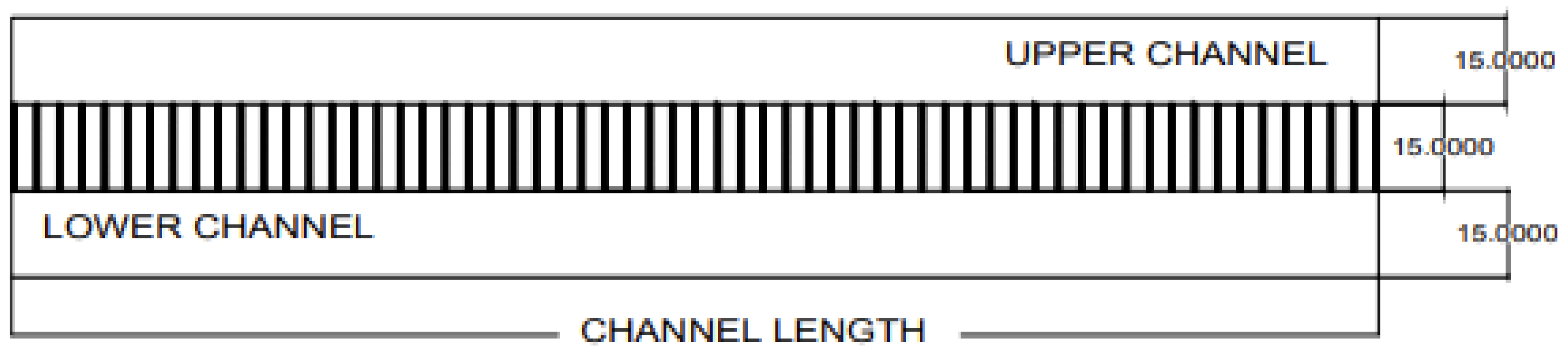
Figure 2.
Counter current flow in channels separated by membrane– Boundary Conditions.
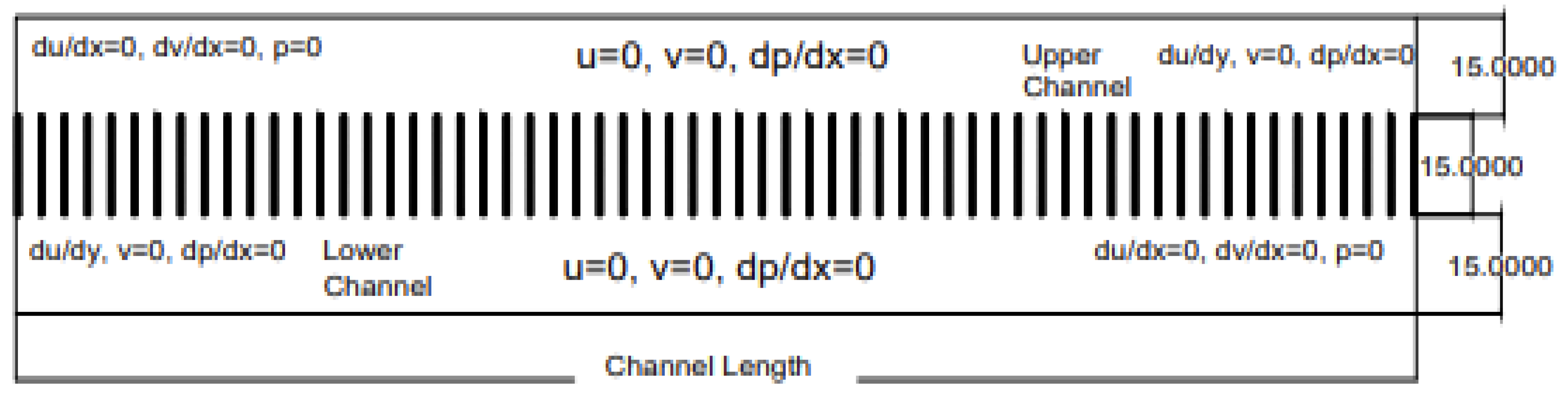
Figure 3.
Horizontal Velocity, Vertical Velocity, and Pressure for Channel Length (60 Holes).
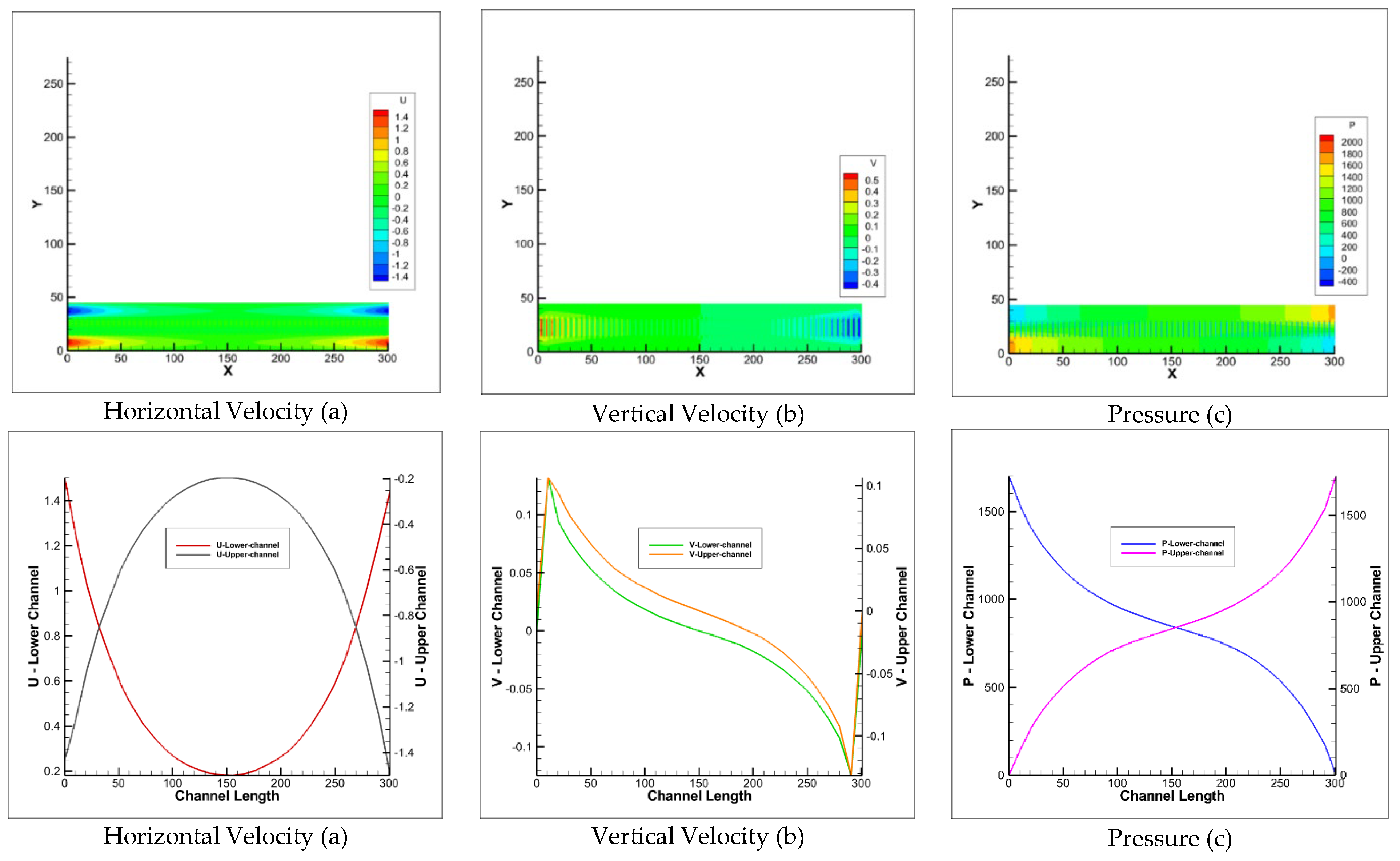
Figure 4.
Pressure, Horizontal velocity, and Vertical velocity along channel length (No. of holes).
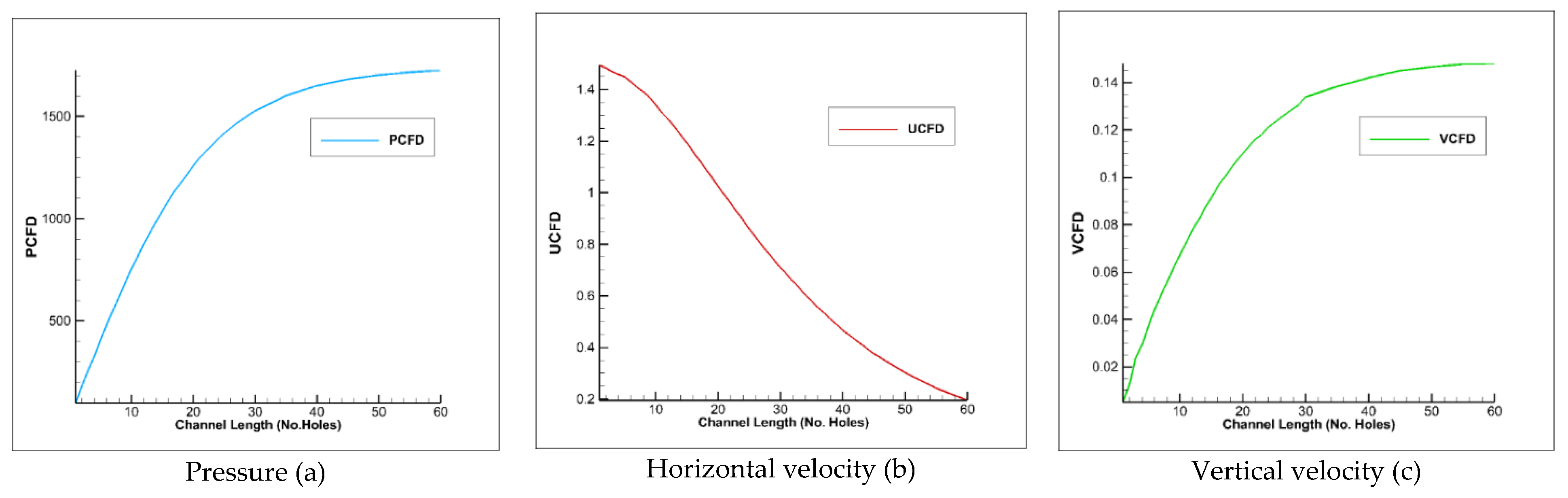
Figure 5.
Non-dimensional pressure (a), horizontal velocity (b) and vertical velocity (c) with non-dimensional length of the channel.
Figure 5.
Non-dimensional pressure (a), horizontal velocity (b) and vertical velocity (c) with non-dimensional length of the channel.
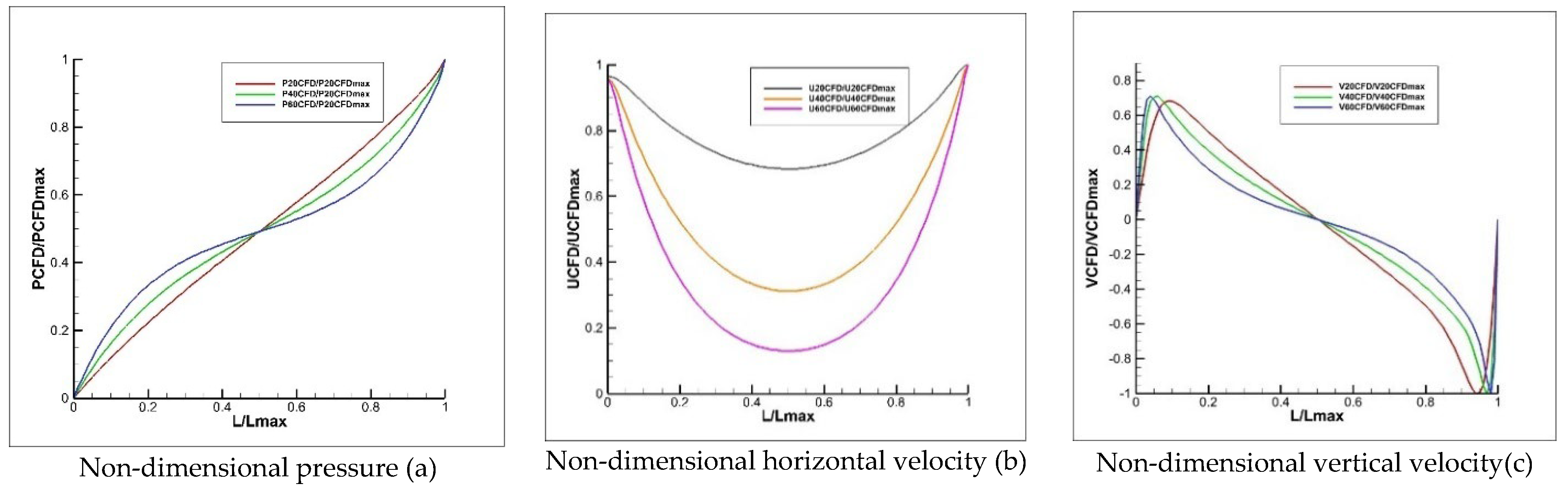
Figure 6.
Comparison of the mean horizontal velocity for the channel length between the models.
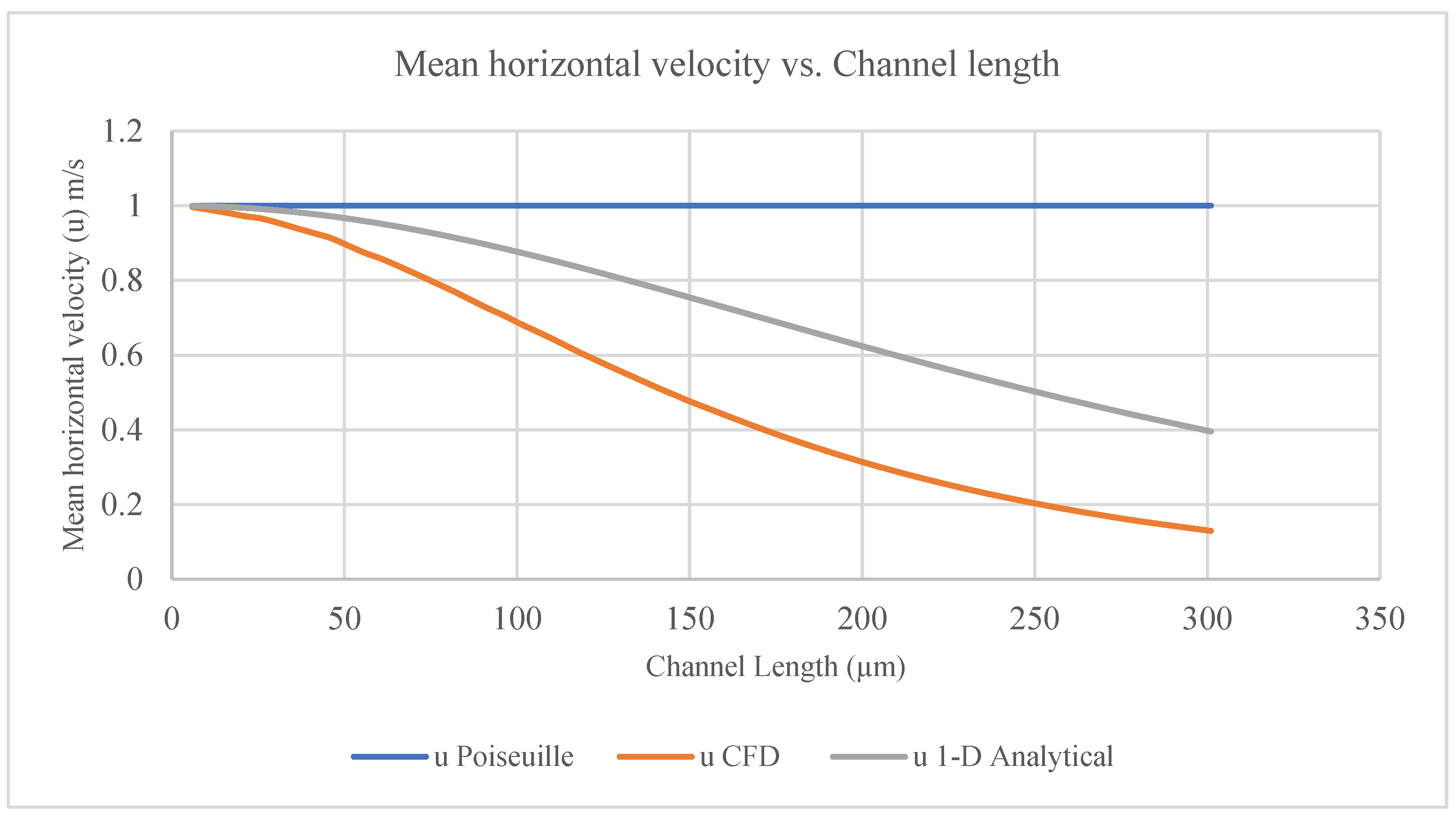
Figure 7.
Comparison of the inlet pressure for the channel length between the models.
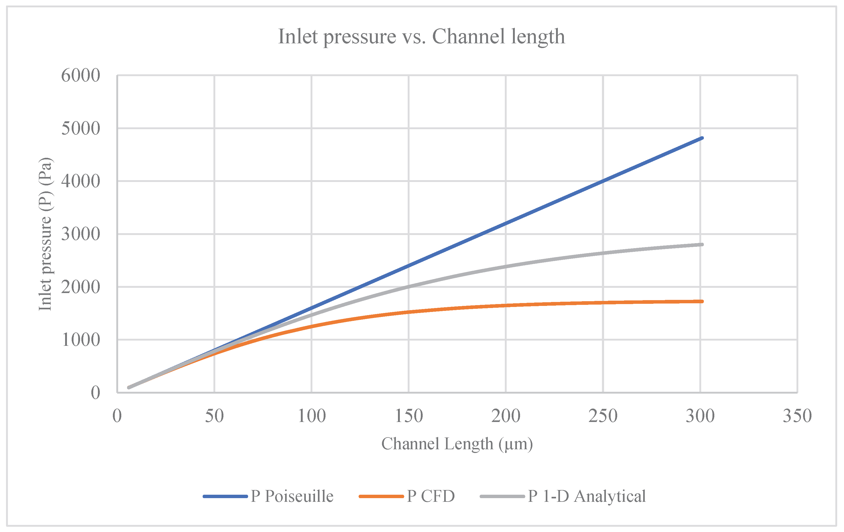

Table 1.
The current study input parameters.
| Parameter | Unit | Values | Notes |
|---|---|---|---|
| The channel (lower and upper) height (hc) | µm | 15 | hc =1.50E-05m |
| The membrane height(hm) | µm | 15 | hm =1.50E-05m |
| The Length of channel (lower and upper) and membrane (L) | µm | 6 - 301 | L = 6.0E-06m - 3.01E-04m |
| Density (ρ) | Kg/m3 | 1000 | water at (40C) |
| Dynamic Viscosity (μ) | [(Pa ·s) =(N·s/m²) = (kg /m.s)] |
3.00E-04 | |
| Kinematic Viscosity (ν) | (m2/s) | 3.00E-07 | ν = μ/ ρ |
| Reynold Number (Re) | - | 3.33E-03 =1/300 | Re = ρ u L/ μ = u L / ν |
| Maximum Horizontal Velocity (umax) | m/s | 1.5 | Assume at inlet |
| Average Horizontal Velocity (umean) | m/s | 1.0 | umean=2/3 umax |
Table 3.
Non-dimensional for horizontal, vertical velocity, and pressure.
| Channel length (No of Holes) | V inlet-CFD | U middle-CFD | U middle-CFD /U maxinlet | PCFD | PANALY | PCFD/PANALY |
|---|---|---|---|---|---|---|
| 101(20) | 0.110 | 1.0252 | 0.683 | 1258 | 1616 | 0.778 |
| 201(40) | 0.142 | 0.467 | 0.311 | 1650 | 3216 | 0.513 |
| 301(60) | 0.148 | 0.194 | 0.129 | 1725 | 4816 | 0.358 |
Where: U max inlet (m/s) (1.5 m/s) =maximum horizontal velocity at inlet of the channel length without membrane (Poiseuille flow). U CFD (m/s) = maximum horizontal velocity at L/2 of the channel length with membrane. V CFD (m/s) = maximum vertical velocity at the inlet of the channel with membrane. P CFD (Pa) = maximum pressure at the inlet of the channel with membrane. P Analytical (Pa) = Analytical pressure at the inlet of the channel without membrane (Poiseuille flow). P Analytical can be calculated by using equation (1). Figure 5 shows the non – dimensional pressure, horizontal velocity, and vertical velocity. Where: P = pressure variation at the inlet of the channel. U = horizontal velocity variation at L/2 of channel length. V = vertical velocity variation along the channel.
Table 4.
2D Permeability (k), Porosity(ɸ), and Hydraulic Permeability (Lp) for 2Dchannels.
| No. | References | Equation | Description |
|---|---|---|---|
| 1 | (Selvam, R.P., 2022) |
K= h2/12 | Permeability / 2D Channel = 1.88E-11 m2 |
| 2 | Hoskins et al., (2024) | Porosity (ɸ) = volume of voids/total volume | Porosity (ɸ) / 2D Channel = 0.64 |
| 3 | (Ciofalo, M., 2023) | Lp = ∆Q/L*w*p | Hydraulic Permeability / 2D channels = 5.16E-05 m/Pa.s |
Table 5.
Comparison between current study and recent related studies.
| Current study 2025 | Cancilla et al., 2022& Ciafalo, 2023 | |
| Channel height (µm) | 15 | 45 (upper channel), 75 (lower channel) |
| Membrane thickness(height) (µm) | 15 | 30 µm |
| Channel length (µm) | 6-301 | 15000 –25000, used (24400) |
| Pore size (R) (µm) | 4.0 | - |
| Fiber inner diameter (D) (µm) | - | 200 No 8000–16,000 |
| Q blood | - | 300 mL/min |
| Q dialysis | - | 500 mL/min |
| Forward velocity (inlet) | 1m/s | - |
| Backward velocity (inlet) | 1m/s | - |
| Forward pressure (inlet) | variable | - |
| Backward pressure (inlet) | variable | - |
| Transmembrane Pressure | 97 Pa (0.14psi) -1725 Pa (2.5psi) | concentration difference |
| Filtration Process | Microfiltration | Ultrafiltration |
Disclaimer/Publisher’s Note: The statements, opinions and data contained in all publications are solely those of the individual author(s) and contributor(s) and not of MDPI and/or the editor(s). MDPI and/or the editor(s) disclaim responsibility for any injury to people or property resulting from any ideas, methods, instructions or products referred to in the content. |
© 2026 by the authors. Licensee MDPI, Basel, Switzerland. This article is an open access article distributed under the terms and conditions of the Creative Commons Attribution (CC BY) license (http://creativecommons.org/licenses/by/4.0/).
Copyright: This open access article is published under a Creative Commons CC BY 4.0 license, which permit the free download, distribution, and reuse, provided that the author and preprint are cited in any reuse.


