
Submitted:
27 January 2026
Posted:
28 January 2026
You are already at the latest version
Abstract
Residuals play a central role in linear regression, but their geometric structure is often obscured by formulas built from matrix inverses and pseudoinverses. This paper develops a rank-aware geometric framework for residual projection that makes the underlying orthogonality explicit. When the design matrix has codimension-one, the unexplained part of the response lies on a single unit normal to the predictor space, so the residual projector collapses to a rank-one operator nn⊤ and no matrix inversion is needed. For general, possibly rank-deficient, designs the residual lies in a higher-dimensional orthogonal complement spanned by an orthonormal basis N, and the residual projector factorizes as NN⊤. Using generalized cross products, wedge products, and Gram determinants, we give a basis-independent characterization of this residual space. On top of this, we introduce the Geometric Multicollinearity Index (GMI), a scale-invariant diagnostic derived from the polar sine that measures how the volume of the predictor space shrinks as multicollinearity increases. Synthetic examples and an illustrative real-data experiment show that the proposed projectors reproduce ordinary least squares residuals, that GMI responds predictably to controlled collinearity, and that the geometric viewpoint clarifies the different roles of regression projection and principal component analysis in both full-rank and rank-deficient settings.
Keywords:
linear regression
; orthogonal projection
; geometric residuals
; multicollinearity
; polar sine
; Gram determinant
; geometric multicollinearity index (GMI)
; null-space
1. Introduction
Linear regression remains one of the most widely used modeling tools in statistics, data science, and machine learning [2]. In its familiar form
The ordinary least squares (OLS) estimator chooses coefficients that minimize the squared discrepancy between observations and predictions. When the design matrix X has the full column-rank, the fitted values and the associated orthogonal projector onto the column space take the classical form
with P symmetric and idempotent [5]. More generally, the orthogonal projector onto can be written as in terms of the Moore–Penrose pseudoinverse [5].
The fitted component and residual are
so that and
is the orthogonal decomposition of the response into a part explained by and a part orthogonal to it. This algebraic formulation is standard, but it can obscure the underlying geometry that governs the behavior of the residuals, and inversion-based formulas can be fragile in high-dimensional or nearly singular regimes [5].
A classical identity from numerical linear algebra makes the geometry explicit:
where the columns of N form an orthonormal basis of [5]. When , the orthogonal complement is one-dimensional and the projector reduces to the rank-one form
where n is the unit vector (ambiguous sign) perpendicular to . In this codimension-one setting, the residual is the projection of Y into a single direction, and the operator (5) completely avoids matrix inversion. For higher-codimension, the residual lies in a subspace of dimension , and the factorization (4) makes this structure explicit.
The construction of normal directions motivates generalizations of the classical cross-product to . Belhaouari et al. formalize a determinant-based vector product that yields a vector orthogonal to linearly independent vectors in [7]. In regression problems with , a single normal vector uniquely defines the rank-one projector (5). For higher-codimensions, these constructions naturally combine with null-space and QR-based methods to form an orthonormal residual basis N.
Multicollinearity is a persistent challenge in regression modeling, as highly dependent predictors inflate variances, destabilize coefficient estimates, and impede interpretation [11]. Classical diagnostics such as the variance inflation factor (VIF) quantify this effect but offer limited geometric insight. We therefore introduce the Geometric Multicollinearity Index (GMI), a scale-invariant, volume-based measure derived from the polar sine and the Gram determinant. For a full column-rank matrix with , the polar sine normalizes by the product of the column norms, taking values in : it equals 1 for orthogonal predictors and approaches 0 as multicollinearity increases.
In rank-deficient or over-parameterized regimes, the Gram determinant vanishes and the GMI saturates at 1, indicating extreme geometric degeneracy. As a normalized volume measure of the parallelotope spanned by the columns of X, the GMI provides a compact, scale-invariant geometric diagnostic across dimensions. In this regime, should be interpreted as a diagnostic flag for complete geometric collapse, rather than as a measure of severity beyond rank deficiency.
Although both regression and principal component analysis (PCA) rely on orthogonal projections, their objectives differ fundamentally [4]. PCA projects X onto directions of maximum variance, yielding residuals that remain in . By contrast, regression projects the response, decomposing Y into a fitted component and a residual [5]. This distinction between feature-space and response-space residuals is essential for interpreting linear-model diagnostics.
Scope of the present paper. The identities and are standard results from orthogonal projection theory. The contribution of this paper lies in a rank-aware geometric interpretation of these identities via multivector and cross-product constructions, together with the introduction of the volume-based Geometric Multicollinearity Index (GMI) as a complementary geometric diagnostic.
This work is theoretical in nature. We develop a rank-aware residual projector, characterize the associated residual subspaces, and formalize GMI as an intrinsic measure of multicollinearity. Algorithmic, large-scale, regularized, and nonlinear extensions are beyond the scope of this paper and are left for future work.
Contributions. The main contributions of this theoretical paper are as follows:
- Rank-aware geometric formulation. We develop a unified, rank-aware description of the residual projector based on the identity , which reduces to the rank-one form when and generalizes to arbitrary rank.
- Multivector perspective on residual spaces. We reformulate and the associated projector using multivectors, wedge products, and cross-products, yielding a basis-independent geometric characterization valid in both codimension-one and higher-codimension settings.
- Geometric Multicollinearity Index (GMI). We introduce a scale-invariant, volume-based diagnostic derived from the Gram determinant and polar sine, which quantifies geometric degeneracy in both full-rank and rank-deficient regimes and complements classical VIF-type measures.
- Regression versus PCA residuals. We clarify the conceptual distinction between regression residuals and PCA reconstruction residuals, emphasizing the impact of projecting the response versus the predictors on residual geometry and interpretation.
- Illustrative examples. We provide simple numerical examples illustrating rank-one and multivector residual projections and the behavior of GMI under controlled perturbations.
Organization of the paper.Section 2 introduces the notation and basic geometric concepts. Section 3 develops the main theoretical results on residual projectors and the geometric structure of . Section 4 presents numerical illustrations, including the behavior of GMI under controlled multicollinearity. Section 5 and Section 6 discuss implications and conclude.
2. Notation and Preliminaries
We briefly fix notation and recall the algebraic and geometric concepts that underpin the proposed framework. We follow standard linear algebra conventions as in Strang [1], Lay et al. [3], and Golub and Van Loan [5].
2.1. Basic Notation and Subspaces
The transpose of a matrix or vector is denoted by the superscript ⊤. Lowercase letters (e.g., x, n) denote column vectors, and uppercase letters (e.g., X, N) denote matrices. For a matrix , we write for its column space and denote its rank by . Throughout, r denotes the residual vector, while denotes the rank of X, to avoid notational ambiguity. All notation is defined once and used consistently throughout the manuscript; in particular, N denotes an orthonormal basis of the orthogonal complement .
We reserve r exclusively for the residual vector in (8).
The orthogonal complement of a subspace is denoted by , and the null-space of a matrix A is
A summary of all symbols and subspace conventions is provided in Abbreviations.
Given , the matrix denotes its outer product. The identity matrix in is denoted by I.
2.2. Projection and Residual Operators
Let have rank ; when X has full column-rank (), the orthogonal projector admits the classical closed form .
The orthogonal projector onto the column space is the unique symmetric idempotent matrix P that satisfies
When X has full column-rank , this projector admits the well-known closed form
which is symmetric and idempotent [5]. In the general case, including rank-deficient designs, P can be written as
where denotes the Moore–Penrose pseudoinverse of X [5].Throughout, denotes the Moore–Penrose pseudoinverse of X, computed via an SVD-based routine.
When , the same orthogonal projector can equivalently be constructed by Cholesky factorization of , producing identical residuals while requiring positive definiteness of the Gram matrix.
For any response vector , the fitted component is
and the residual is
which obeys and hence lies in the orthogonal complement [5].
Let and set . Choose any matrix whose columns form an orthonormal basis of :
Then the residual projector admits the geometric factorization
and the null-space of is
This characterization is standard in numerical linear algebra and regression theory [5] and forms the algebraic backbone of our geometric residual formulation. Equation (10) makes explicit that the residual r lies in a k-dimensional orthogonal complement spanned by the columns of N.
2.3. Cross-Product and Cross–Wedge–QR Method
To construct explicit orthogonal directions, especially in the case of codimension-one where , we employ the cross-product in [7]. Given linearly independent vectors
the determinant-based construction of Belhaouari et al. produces
which is orthogonal to each :
This extends earlier n-dimensional vector products and related constructions in eigenanalysis and geometry [8,9].
In the regression setting, when the predictor space has codimension one and is spanned by a single unit vector n. Choosing any basis of and applying the cross-product yields a nonzero vector orthogonal to ; normalizing it gives a unit normal n spanning . In this case, the residual projector reduces to the rank-one form
and the residual is simply .
In this codimension-one setting, the rank-one projector coincides with the classical construction of the cross-product, and we refer to this case as the residual projector of the cross-product (rank-one).
A key geometric property of the cross-product is that its norm equals the -dimensional volume of the parallelotope spanned by its arguments [7]:
Thus, the cross-product simultaneously provides an orthogonal direction and encodes a volume. When , a single cross-product yields at most one null direction; in that case additional null directions must be obtained by other means (e.g., null-space methods and QR), as discussed later.
2.4. Wedge Products, Gram Matrices, and Polar Sine
To describe volumes and linear independence in a coordinate-free manner, we rely on standard constructions from linear algebra and multilinear geometry [1,3,5]. Given vectors , their wedge product encodes the oriented k-dimensional parallelotope spanned by . Geometrically, if and only if the vectors are linearly dependent, and its norm equals the volume k of the associated parallelotope. This interpretation underlies many geometric treatments of subspaces, volumes, and orthogonality in [1,5].
For computational purposes, such volumes can be expressed using Gram matrices. Given vectors , the associated Gram matrix is
The m-dimensional volume of the parallelotope spanned by is given by
a classical identity that plays a central role in covariance analysis and principal component analysis [4,5].
We quantify the angular separation of p predictor vectors using the polar sine. Let with Gram matrix . Following geometric constructions based on determinants and cross-products [7,8,9], the polar sine is defined as
When and the columns of X are linearly independent, and ; it equals 1 if and only if the vectors are mutually orthogonal. If the columns of X are linearly dependent or , then is singular and , and we adopt the convention . Thus, the polar sine takes values in , is scale-invariant, and decreases toward zero as the set of columns becomes geometrically degenerate.
Within the present framework, the polar sine provides a normalized geometric measure of predictor-space collapse under multicollinearity and forms the basis of the Geometric Multicollinearity Index (GMI) introduced in the following section.
2.5. Projection Strategies: QR and Cross-Product Formulations
Two projection strategies play a central role in the remainder of the paper.
First, QR decomposition is used when an entire orthonormal basis of or is required. If is a (thin) QR factorization with orthonormal columns in Q, then
is the orthogonal projector onto , and orthonormal complements can be obtained by extending Q to an orthogonal basis of [5]. QR-based projectors are numerically stable and well suited for high-dimensional or nearly singular problems.
Second, when the residual space is one-dimensional (for example, when ), the cross-product provides a compact alternative. It produces a normal vector n directly from which the residual projector is derived:
This follows without forming or inverting [7]. In higher-codimension settings (), cross-products can still be used to generate individual null directions, but a full residual basis is obtained more naturally from and orthonormalised via QR.
When null directions are generated sequentially via cross-products and accumulated into a multivector basis that is subsequently orthonormalised using QR, we refer to the resulting construction as the Recursive Cross–Wedge–QR method.
These geometric primitives—orthonormal bases, cross-products, wedge products, Gram matrices, and polar sine—constitute the toolkit on which the residual projection framework developed in the following sections is built.
Here s denotes the sketch size (number of random probe vectors) used in the Gaussian range-finding procedure.
2.5.0.1. Sketch–QR Baseline (Reproducibility)
The Sketch–QR baseline follows a standard randomized range-finding procedure. Given and a sketch size s, we draw a Gaussian sketching matrix with i.i.d. entries and form . We then compute a thin QR factorization , where has orthonormal columns. The approximate projector is , and the approximate residual is . Unless stated otherwise, we use a single sketch without power iterations or oversampling [6,16].
3. Core Theory
3.1. Rank-One Residual Projection
Assume that has rank . Then and . There exists a (unique up to sign) unit vector such that
Proposition 1 (Rank-One Residual Projection).
Let have , and let P denote the orthogonal projector onto (for example, in terms of the Moore–Penrose pseudoinverse ). Then the orthogonal residual projector is
Proof.
Because is one-dimensional, any residual can be written as for some scalar . Since and P is the orthogonal projector onto , we have and therefore . For any , we may write with and . Then
while
because and v is a scalar multiple of n. Thus for all Y, and therefore , which is symmetric and idempotent. □
3.2. Generalization to n Dimensions
The rank-one projector extends naturally to the general setting in which the predictor matrix has . In this case the orthogonal complement has dimension , and the residual is no longer confined to a single direction but lies in a k-dimensional subspace.
Theorem 2 (Multivector Residual Projection).
Let X have rank and set . Let have orthonormal columns spanning (so ). Then the residual projector is and .
Proof.
Since , the matrix is symmetric and satisfies
so is an orthogonal projector. Its range equals .
On the other hand, P is the orthogonal projector onto , so is the orthogonal projector onto . For any , write with and . Then
Since and the columns of N are orthonormal, we also have
because and acts as the identity on . Thus for all Y, and hence . □
Figure 1 illustrates the situation in a simple three-dimensional example. The predictor space occupies a lower-dimensional subspace (blue), while the residual lies in its orthogonal complement (orange), spanned by multiple orthonormal directions when .
3.2.1. Geometric Multicollinearity Index (GMI)
The multivector formulation of the residual projector reflects the angular configuration of the columns of X. When the predictors are nearly linearly dependent, the volume of the parallelotope spanned by these columns collapses, signaling instability. To capture this behavior geometrically, we introduce the Geometric Multicollinearity Index (GMI), a scale-invariant measure based on the polar sine.
Definition 1 (Polar Sine and GMI).
Let have nonzero columns , and let be the polar sine defined in Equation (16)
. We adopt the shorthand
and define the Geometric Multicollinearity Index by
Lemma 3 (Basic properties).
Let have nonzero columns, and let denote its Gram matrix. Then:
- i)
- and hence ;
- ii)
- (and ) if and only if the columns of X are mutually orthogonal;
- iii)
- (and ) whenever the columns are linearly dependent or .
Proof.
By Hadamard’s inequality,
with equality if and only if the columns of X are mutually orthogonal. Substituting this bound into the polar-sine definition Equation (16) yields
which proves (i). Moreover, holds precisely when equality in Hadamard’s inequality holds, i.e., when the columns are pairwise orthogonal, giving (ii).
If the columns of X are linearly dependent or , then G is singular and , so by definition in that case, and (iii) follows immediately. The corresponding statements for are then direct consequences of the definition . □
Lemma 4 (Scale invariance).
Let with each . Then and hence .
Proof.
Remark 1.
For orthonormal predictors, and . For nearly collinear predictors, , so and . Intermediate angular configurations (e.g., vectors separated by ) yield values such as and , as illustrated in Figure 2. In this sense, GMI is a normalized version of determinant-based multicollinearity measures (such as the generalized variance or det of the correlation matrix), rescaled to lie in and made explicitly scale-invariant via the polar-sine normalization.
GMI provides a direct geometric diagnostic that complements classical VIF-type measures. Whereas VIF assesses how much the variance of each individual regression coefficient is inflated by linear dependence among the predictors, GMI treats the entire predictor set as a single geometric object and summarizes its angular degeneracy in a single number in . Because it depends only on the angular configuration of the predictors and is invariant under independent rescaling of the columns, it can be compared meaningfully across differently scaled datasets.
3.2.2. Uniqueness of the Residual Projection
The multivector formulation expresses the residual projector in terms of any orthonormal basis of the orthogonal complement . The next result confirms that this projector is independent of the specific basis chosen.
Remark 2 (Independence of the residual projector from the basis).
Let have rank , and let have orthonormal columns spanning . Then there exists an orthogonal such that , and hence
In particular, the representation from Theorem 2 is independent of the orthonormal basis chosen of : it is simply the (unique) orthogonal projector onto .
3.3. Generalized Projection in Rank-Deficient Spaces via Null-Spaces and Wedge Products
When the design matrix X is rank-deficient or when , the orthogonal complement has dimension greater than one, and a single normal vector—as in the rank-one case—is no longer sufficient to describe the residual direction. In such settings, a full orthonormal basis of is required. This subsection explains how standard null-space computations, combined with QR orthonormalization, yield such a basis, and how wedge products provide a coordinate-free way to reason about independence and volume.
Definition 2 (Residual Projection in the Rank-Deficient Case).
Let have rank , and set . If has orthonormal columns spanning , then the residual projector is
Proposition 5 (Limitation of the cross-product).
The cross-product of Belhaouari [7] produces a single vector orthogonal to independent vectors in . This suffices when , but for it yields only one null direction. Additional directions are needed to span the entire residual space.
Proof.
If , then is one-dimensional, and a single cross-product applied to a basis of recovers the unique (up to sign) normal vector n, giving as in the rank-one case. When , the orthogonal complement has dimension , so multiple linearly independent null directions are required. A single cross-product produces at most one such direction and therefore cannot span a k-dimensional space. Additional vectors must be constructed, for instance, via null-space computations and subsequent orthonormalization. □
Theorem 6 (Construction of a Residual Basis via null-space and QR).
Let have rank r and set , so that has dimension k. Then there exists an orthonormal basis of such that
where P is the orthogonal projector onto . Moreover, such an N can be obtained by the null-space + QR procedure in Algorithm 1.
Proof.
By construction, the columns of B span , which is equal to . If then the ’s are linearly independent and form a basis of this k-dimensional subspace. The thin QR factorization with orthonormal columns in Q then produces with and . The matrix is therefore the orthogonal projector onto , so by the uniqueness of the orthogonal projector onto a fixed subspace. □
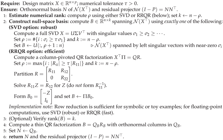
| Algorithm 1 Residual Projector via Null-Space and QR (Explicit SVD/RRQR) |
 |
Remark 3.
In practice, the null-space basis in Step 1 is typically obtained from a numerically stable factorization such as SVD or a rank-revealing QR. The wedge product need not be computed explicitly; it serves primarily as a geometric way to interpret the independence check. When , the construction reduces to the case of rank-one , where a normal vector can be obtained either from the null-space of or by applying a cross-product to a basis of .The numerical tolerance used for the determination of rank (e.g., relative to the largest singular value) follows standard practice and does not affect the conceptual geometric results, which hold exactly at the algebraic level.
Remark 4 (Implementation note: computing in floating-point arithmetic).
The instruction “compute a basis of ” requires (i) a numerical rank decision and (ii) an explicit extraction rule. In this work we use either:
(a) SVD. Compute , choose the numerical rank , and set .
(b) RRQR. Compute a column-pivoted QR factorization , choose rank ρ from the diagonal of R (e.g., ), partition , and set .
SVD is typically more robust under severe ill-conditioning, while RRQR is often faster when pivoted QR is sufficient. Row-reduction is used only for symbolic/toy demonstrations.
Figure 3 illustrates the residual subspace and two independent null directions before orthonormalization.
3.4. Projection Method Variants and Complexity
Definition 3 (Variants of Residual Projection).
Let be a real-valued design matrix of rank . The residual projection operator onto the orthogonal complement can be constructed by several exact procedures, each suited to different regimes of dimension, conditioning, and interpretability.
The following variants highlight that null-space, wedge-based, and determinant-based approaches provide geometrically transparent alternatives to inversion-based formulas in linear regression.
Proposition 7 (Wedge–QR Null-Space Variant).
Let have rank ρ, and let . Using the null-space + QR construction of Theorem 6, we obtain an orthonormal residual basis spanning and hence the projector . If, in addition, we compute a thin QR factorization , then the Gram matrix satisfies
so the squared volume of the parallelotope spanned by the columns of X is given directly by . The general complexity of forming N and R is .
Proof.
The existence of an orthonormal basis N of and the identity follow from Theorem 6. The factorization implies , so , which yields the stated volume formula. The complexity estimate is inherited from the null-space + QR construction. □
When geometric interpretations involving volume are necessary-such as evaluating multicollinearity through the Geometric Multicollinearity Index (GMI)—factorizations of the Gram matrix are particularly convenient.
Proposition 8 (Cholesky-Based Volume and Projection).
Let and assume that X has full-column-rank so that . Compute the Cholesky factorization , which yields
Let N be any orthonormal basis of constructed as in Theorem 6. Then is the orthogonal residual projector. The dominant cost is : for the Cholesky factorization and for forming and applying N.
Proof.
The positive definiteness of G ensures the existence of a unique Cholesky factor L with positive diagonal entries, and the determinant formula follows from . The construction of N and the identity is provided by Theorem 6; any such N produces an orthogonal projector onto . □
In the special case where the residual subspace is one-dimensional, the projector admits an especially simple representation.
Proposition 9 (cross-product (Rank-One Case)).
If , then
where satisfies and . The one-time cost of building n is , and each subsequent projection costs .
Proof.
When is one-dimensional, any nonzero vector in this space is a scalar multiple of a unit normal n. The orthogonal projector onto the line spanned by n is precisely . Symmetry and idempotence follow from , and orthogonality is ensured by . □
Example 1.
Consider , , and the residual-codimension . In this codimension-one setting, the classical OLS residual projector based on (assuming that X has full column-rank) involves a matrix inversion together with several matrix–vector multiplications, which require on the order of a few hundred floating-point operations in this small example. By contrast, computing a unit normal vector n via the geometric cross-product costs operations, and each application of the rank-one projector to a new response Y costs only operations. Once n has been constructed, the projection of additional responses is therefore substantially cheaper than recomputing residuals through , illustrating the efficiency of geometric formulation in symbolic or resource-limited regimes.
Unless stated otherwise, we use a single Gaussian sketch without power iterations or oversampling; orthonormalization is performed via a standard thin QR factorization.
| Algorithm 2: Sketch–QR Baseline (Gaussian Range Finder) |
 |
Table 1 compares four exact ways to build the residual projector for a given design matrix X. Classical OLS and the Cholesky-based variant both work through and treat the residual subspace only implicitly, with a cubic dependence on the number of predictors p and the restriction that be invertible. In contrast, the Wedge–QR and rank-one cross-product methods construct from an explicit basis of ; the former handles general rank-deficient cases, while the latter is tailored to the codimension-one setting and achieves the lowest per-response cost when many responses must be projected.
In summary, Wedge–QR and Cholesky-based constructions are well-suited when one needs both an exact residual projector and access to volume-based quantities such as or the GMI. The formulation of a rank-one cross-product is preferable whenever , as it produces a simple geometric projector with linear complexity per response and, when , is usually the cheapest option to repeatedly project many responses. For general rank-deficient designs, a QR/null-space construction offers a numerically safer alternative to explicitly forming and inverting . Together, the four variants in Table 1 provide a practical menu of exact geometric projectors that avoid unnecessary matrix inversion and can be chosen according to the rank of X, the conditioning of and the available computational budget.
We emphasize that the exact residual projector can be constructed via several algebraically equivalent routes (normal-equations OLS when applicable, rank-one cross products, null-space/QR, wedge-based constructions and Cholesky-based variants), which differ only in numerical assumptions and computational cost; see Table 1.
4. Illustrative Numerical Examples
When the design matrix X is rank-deficient, the normal equations do not admit a unique solution. In all rank-deficient experiments, we therefore compute the minimum-norm least-squares solution using the Moore–Penrose pseudoinverse, i.e., , and refer to this baseline as OLS (Moore–Penrose pseudoinverse).
Evaluation protocol. Predictive performance is assessed using K-fold cross-validation with , reporting CV MSE and CV . Unless stated otherwise, all randomized procedures use a fixed random seed (seed = 42) to ensure reproducibility.
Coefficient-stability summary. Coefficient stability is evaluated via perturbation trials with the design matrix X held fixed. In each trial, the response is perturbed as
The model is refit for each trial to obtain coefficients . Let denote the sample standard deviation of the jth coefficient across trials. We summarize coefficient stability by
i.e., the median across coefficients of their across-trial standard deviations.
To validate the geometric projector, we verify agreement between the classical OLS residual and the geometric residual by monitoring up to numerical tolerance.
Sketch–QR [6] yields an approximate basis and projector , producing the approximate residual . Agreement with the exact residual is summarized using cosine similarity and the residual discrepancy (and, when reported, a principal-angle distortion between and ).
4.1. Rank-One Residual Projection in
This example explicitly shows how the normality of the cross-product reproduces the ordinary least-squares (OLS) residual in the rank-one case, in line with Proposition 1.
We consider a rank-one residual setting where the orthogonal complement of the column space is one-dimensional. Let us
with of full-column-rank (so is invertible). The ordinary least-squares projection matrix is
A direct calculation yields
To recover the same residual in purely geometric form, we construct a unit normal vector to the column space of . Let us
Then and , so Proposition 1 applies, and
The residual can therefore be written as the rank-one projection
which coincides with and lies on the line spanned by .
From a computational point of view, this example highlights the attraction of the geometric formulation in low dimension: the cross-product and the multiplication of a scalar vector are sufficient to obtain the residual, avoiding explicit matrix inversion. Once is known, applying the projector to a new response vector reduces to one dot product and one scaled copy of , i.e., work per residual.
4.2. Multivector Residual Projection in
This example illustrates the multivector residual projection via an orthonormal basis of as in Theorem 6, and links it to the Geometric Multicollinearity Index.
We now consider a multivector setting in which the residual subspace has a dimension greater than one. Let us
The ordinary least-squares projector is again
and a straightforward computation gives
Since , its orthogonal complement has dimension . A basis for the null-space of is
Applying Gram–Schmidt yields an orthonormal basis
with and . The general residual projection theorem then gives
Evaluating for this and reproduces the residual OLS:
making explicit that the residual lives in the two-dimensional subspace spanned by and and realizing the null-space + QR construction in Theorem 6, in a concrete low-dimensional setting.
From a complexity point of view, building on a null-space basis followed by QR (or Gram–Schmidt) is a one-off cost of order for with residual dimension , while applying the projector to a new response vector requires only operations.
4.2.0.1. GMI for the Example
For this design matrix , the Gram matrix is
The column norms are and , so the polar sine and the Geometric Multicollinearity Index are
In this small example, the GMI value indicates a moderate degree of collinearity between the two regressors; the residual subspace has dimension two (as ), and, compared to the orthonormal case (), the fitted coefficients are more sensitive to perturbations of .
This example isolates the effect of controlled collinearity on GMI in a minimal symbolic setting.
Consider the family of matrices
For every the two columns are linearly independent, so is positive definite, and the polar-sine is well-defined. A direct computation gives
and hence
As increases, the columns become more collinear, decreases, and increases, reflecting the growing multicollinearity in a purely geometric way. In families where columns eventually become exactly collinear, the Gram determinant vanishes, the polar sine drops to zero, and reaches 1, in agreement with the rank-deficient discussion in Section 3.
4.2.0.2. Large-Scale Multivector Residual Projection
To complement the low-dimensional symbolic example above, we consider a larger synthetic design in which the residual subspace has a dimension greater than one and the multivector formulation is essential.
We generate a rank-deficient design matrix with , , and , so that . All predictors are standardized, and the response is constructed so that the exact residual has a prescribed norm, ensuring a controlled comparison between methods.
Table 2 reports residual norms, cosine similarity to the exact residual, and run times for the variants of the Article 1 projector only. The exact constructions (null-space/QR, rank-one cross-product when applicable, and the Moore–Penrose pseudoinverse baseline for OLS) reproduce the same residual up to numerical precision, confirming the multivector identity in a high-dimensional setting.
Sketch–QR yields an approximate residual, whose agreement with the exact residual is summarized by cosine similarity.Entries marked NaN or N/A indicate methods that are not applicable in this regime (e.g., rank-one cross-product when ), while FAIL indicates that the required algebraic conditions (e.g., ) are violated.
This experiment demonstrates that the geometric residual formulation extends naturally from symbolic low-dimensional examples to realistic large-n, rank-deficient designs, without relying on regularization or nonlinear modeling.
Together with the symbolic R4 example, this large-scale synthetic experiment confirms that the multivector residual projector is exact in dimensions, while Sketch–QR provides a principled approximation when a reduced basis is desired, setting the stage for the real-data illustrations in Section 4.3.
4.3. Illustrative Real Data Use of GMI
Real-data experiments use two regression benchmarks: Boston Housing and Auto MPG. Both are standardized via centering and scaling before forming X, and they provide realistic multicollinearity patterns suitable for illustrating GMI as a purely geometric, response-independent diagnostic.
This example illustrates how GMI can serve as a purely geometric multicollinearity diagnostic on real data and how it can be interpreted alongside coefficient stability.
We use the Boston Housing dataset because it is a widely used regression benchmark with well-known predictor correlations, making it a convenient setting for illustrating multicollinearity diagnostics and residual geometry on realistic data.
To illustrate the geometric diagnostics on real data, we use the classical Boston Housing dataset, with median house price as the response and a set of standardized socio-economic and structural predictors. The protocol used in this subsection is as follows:
- (a)
- Standardise all predictors to zero mean and unit variance, and form the design matrix X.
- (b)
- For selected subsets of predictors, form the corresponding design matrix X, compute the Gram matrix , and evaluate the polar sine and GMI using the definitions in (18).
- (c)
- Report predictive metrics using 5-fold cross-validation (CV) so that MSE and are out-of-sample summaries rather than in-sample fit statistics.
- (d)
- Fit ordinary least-squares models on these subsets and monitor the variation of the estimated coefficients under small perturbations of Y (e.g., additive Gaussian noise or resampling).
The purpose of this subsection is to demonstrate (i) that the geometric residual projector reproduces the classical OLS residuals on a realistic dataset, and (ii) that GMI provides a compact, response-independent summary of predictor-space degeneracy.
4.3.0.3. Boston Housing and Auto MPG: Increasing Model Size
Real-data experiments use two regression benchmarks: Boston Housing and Auto MPG. Both are standardized through centering and scaling before forming X, and provide realistic multicollinearity patterns suitable to illustrate GMI as a purely geometric and response-independent diagnostic.
Table 3 and Table 4 report results for increasing the size of the model (, , , and in full where applicable). For each subset, we report out-of-sample predictive metrics using 5-fold cross-validation (CV MSE and CV ), geometric multicollinearity (GMI), and classical diagnostics (max VIF and ), along with a summary of coefficient-stability.
We restrict algorithmic comparisons to the projector variants defined in Table 1 (OLS/Cholesky when applicable, null-space/QR, rank-one cross-product when , and Sketch–QR).
Table 3Table 4 show that increasing the size of the model improves predictive performance (lower CV MSE, higher CV ) while typically increasing multicollinearity. In Boston, moving from to the full model reduces CV MSE from to and increases CV from to , while GMI increases from 0 to and increases from 1 to . In Auto MPG the collinearity is even stronger: the full model attains CV MSE and CV , but the corresponding diagnostics are GMI , max VIF , and .
These results illustrate the intended role of GMI: it is computed purely from X (independent of Y) and tracks familiar multicollinearity measures (VIF and condition number), while the coefficient-stability summary provides a concrete link between predictor-space degeneracy and sensitivity of fitted parameters.
4.3.0.4. Implementation Note (Stable GMI Computation)
When the Gram matrix is poorly conditioned, the evaluation of direct determinants is numerically fragile. We therefore compute the polar sine and GMI in the log-domain with a small jitter :
In implementation, is evaluated using a numerically stable log-determinant routine (equivalently, a Cholesky factorization when ). Unless stated otherwise, we use .
Figure 4 makes the equivalence of the exact geometric projector and classical OLS residuals explicit: the discrepancy curve for the exact QR-basis construction is at a numerical noise level in both the and models. In contrast, Sketch–QR constructs an approximate projector , so its residual differs slightly from ; the magnitude of this discrepancy decreases as the size of the sketch s increases. Overall, this visualization complements Table 3Table 4 by separating the exact residual-geometry identities (Article 1 methods) from the approximate Sketch–QR construction while keeping the presentation compact and reproducible.
5. Discussion
This paper presents a rank-aware geometric interpretation of linear regression residuals via orthogonal projectors. In the case of codimension-one, the residual is fully determined by a unit normal , resulting in ; in general rank settings, the residual lies in a higher-dimensional orthogonal complement spanned by an orthonormal basis N, with . This formulation makes the residual subspace explicit and decouples basis construction from repeated projection.
An immediate consequence is that all exact computational routes—normal-equation OLS, Cholesky-based solvers, and null-space or QR constructions—must yield identical residuals up to numerical tolerance, as they implement the same projector onto . We confirm this numerically through residual agreement metrics and discrepancy visualizations, showing that differences arise only from conditioning and the computational regime. In contrast, Sketch–QR yields an approximate projector and residual, whose deviation from the exact solution is quantified using cosine similarity and norm-based discrepancies.
We further link residual geometry to predictor-space conditioning through the Geometric Multicollinearity Index (GMI), a scale-invariant, normalized volume measure derived from the polar sine. Across the Boston Housing and Auto MPG benchmarks, higher GMI values consistently align with larger max VIF and , while coefficient-stability summaries illustrate increased parameter sensitivity under geometric degeneracy.
Although both regression and PCA rely on orthogonal projections, their objectives differ fundamentally: PCA projects predictors to minimize reconstruction error, with residuals remaining in , whereas regression projects the response, yielding residuals in .
Finally, this work focuses on unregularized least squares and exact orthogonal projection. With regularization, the operators are no longer orthogonal and the residual subspace becomes non-Euclidean or data-adaptive, motivating future work on regularized and sketch-aware residual geometry while preserving the geometric diagnostics enabled by GMI.
6. Conclusions
This paper presented a rank-aware geometric interpretation of linear regression residuals. In the case of codimension-one, the residual projector reduces to the rank-one form , where n spans . For general rank, the residual lies in a dimensional orthogonal complement, with a projector for an orthonormal basis N of . Although algebraically equivalent to the classical OLS formulation, this representation makes the residual subspace explicit and decouples basis construction from repeated projection.
Building on this viewpoint, we introduced the Geometric Multicollinearity Index (GMI), a scale-invariant diagnostic derived from the polar sine and Gram determinant that quantifies predictor-space degeneracy. Synthetic experiments confirm predictable behavior under controlled perturbations, while real-data benchmarks on Boston Housing and Auto MPG show that increasing model size typically improves predictive performance while increasing multicollinearity; GMI captures this trade-off and aligns with max VIF and . Across all experiments, exact projector constructions yield identical residuals up to numerical tolerance, whereas Sketch–QR produces a controlled approximation whose deviation is quantified via cosine similarity and residual discrepancy norms.
In general, these results elevate to a central geometric object in regression analysis and position GMI as a concise indicator of departure from orthogonal designs. Extensions to sketch-based, large-scale, streaming, and nonlinear settings are deferred to companion work.
Author Contributions
Conceptualization, M.H.A. and S.B.B.; methodology, M.H.A.; formal analysis, M.H.A.; writing—original draft preparation, M.H.A.; writing—review and editing, M.H.A. and S.B.B.; supervision, S.B.B. All authors have read and agreed to the published version of the manuscript.
Funding
This research received no external funding.
Institutional Review Board Statement
Not applicable.
Informed Consent Statement
Not applicable.
Data Availability Statement
Publicly available datasets were analysed in this study. The Boston Housing dataset is available from Kaggle [12] and was originally introduced by Harrison and Rubinfeld [14]. The Auto MPG dataset is available from the UCI Machine Learning Repository [15]. No new data were created. The code used to reproduce the experiments and tables in this manuscript is publicly available as a GitHub repository [13].
Acknowledgments
The authors gratefully acknowledge the academic support of Hamad Bin Khalifa University and Lusail University. They also thank Qatar National Library (QNL) for access to scholarly resources and research databases essential to this study.
Conflicts of Interest
The authors declare no conflicts of interest.
Abbreviations
The following abbreviations are used in this manuscript:
| OLS | Ordinary Least Squares |
| GMI | Geometric Multicollinearity Index |
| PCA | Principal Component Analysis |
| VIF | Variance Inflation Factor |
| CV | Cross-Validation (K-fold) |
| QR | QR (Orthogonal–Triangular) Decomposition |
| RRQR | Rank-Revealing QR Decomposition |
| SVD | Singular Value Decomposition |
| FLOPs | Floating-Point Operations |
| GRP | Geometric Residual Projection |
References
- Strang, G. Introduction to Linear Algebra; Wellesley–Cambridge Press: Wellesley, MA, USA, 1993. [Google Scholar]
- Hastie, T.; Tibshirani, R.; Friedman, J. The Elements of Statistical Learning, 2nd ed.; Springer: New York, NY, USA, 2009. [Google Scholar] [CrossRef]
- Lay, D.C.; Lay, S.R.; McDonald, J.J. Linear Algebra and Its Applications, 5th ed.; Pearson: Boston, MA, USA, 2016. [Google Scholar]
- Jolliffe, I.T.; Cadima, J. Principal component analysis: A review and recent developments. Philos. Trans. R. Soc. A 2016, 374, 20150202. [Google Scholar] [CrossRef] [PubMed]
- Golub, G.H.; Van Loan, C.F. Matrix Computations, 4th ed.; Johns Hopkins University Press: Baltimore, MD, USA, 2013. [Google Scholar]
- Mahoney, M.W. Randomized algorithms for matrices and data. Found. Trends Mach. Learn. 2011, 3, 123–224. [Google Scholar] [CrossRef]
- Belhaouari, S.; Kahalan, Y.C.; Aksikas, I.; Hamdi, A.; Belhaouari, I.; Haoudi, E.M.N.; Bensmail, H. Generalizing the cross-product to N Dimensions: A Novel Approach for Multidimensional Analysis and Applications. Mathematics 2025, 13, 514. [Google Scholar] [CrossRef]
- Mortari, D. n-Dimensional cross-product and its application to matrix eigenanalysis. J. Guid. Control Dyn. 1996, 20, 509–515. [Google Scholar] [CrossRef]
- Walsh, B. The scarcity of cross-products on Euclidean spaces. Am. Math. Mon. 1967, 74, 188–194. [Google Scholar] [CrossRef]
- Kim, J.H. Multicollinearity and misleading statistical results. Korean J. Anesthesiol. 2019, 72, 558–569. [Google Scholar] [CrossRef] [PubMed]
- Chan, J.Y.-L.; Leow, S.M.H.; Bea, K.T.; Cheng, W.K.; Phoong, S.W.; Hong, Z.-W.; Chen, Y.-L. Mitigating the multicollinearity problem and its machine learning approach: A review. Mathematics 2022, 10, 1283. [Google Scholar] [CrossRef]
- Kaggle. Boston Housing Dataset. Available online: https://www.kaggle.com/datasets/altavish/boston-housing-dataset (accessed on 21 November 2025).
- Alkhateeb, M.H.; Belhaouari, S.B. Geometric Residual Projection (GRP): Reproducible Code and Experiments; GitHub repository, 2025. Available online: https://github.com/MaisAlkhateeb/Geometrics-Residual-Projection (accessed on 16 January 2026).
- Harrison, D.; Rubinfeld, D.L. Hedonic prices and the demand for clean air. J. Environ. Econ. Manag. 1978, 5, 81–102. [Google Scholar] [CrossRef]
- UCI Machine Learning Repository. Auto MPG Data Set. University of California, Irvine, School of Information and Computer Sciences, 1993. Available online: https://archive.ics.uci.edu/dataset/9/auto+mpg (accessed on 16 January 2026).
- Halko, N.; Martinsson, P.-G.; Tropp, J.A. Finding structure with randomness: Probabilistic algorithms for constructing approximate matrix decompositions. SIAM Rev. 2011, 53, 217–288. [Google Scholar] [CrossRef]
Figure 1.
Geometric interpretation of the residual projection in a three-dimensional example with and . The design matrix X has a one-dimensional column space (blue line), while the residual space is a two-dimensional plane (orange), spanned by an orthonormal basis . For a response vector , the residual is its orthogonal projection onto .
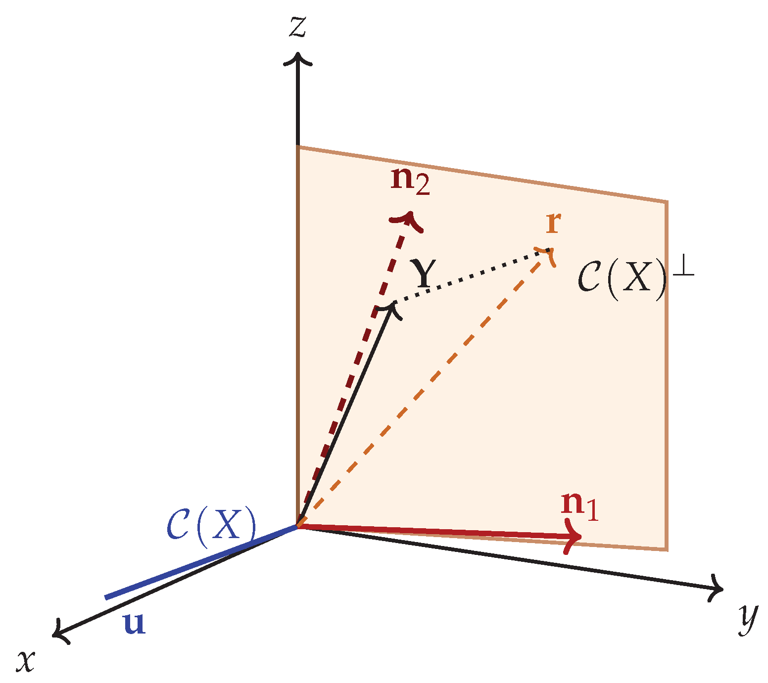
Figure 2.
Geometric Multicollinearity Index (GMI) as a function of the polar sine. The index is zero for orthonormal predictors, increases steadily as angular separation decreases, and approaches one under near-collinearity.
Figure 2.
Geometric Multicollinearity Index (GMI) as a function of the polar sine. The index is zero for orthonormal predictors, increases steadily as angular separation decreases, and approaches one under near-collinearity.
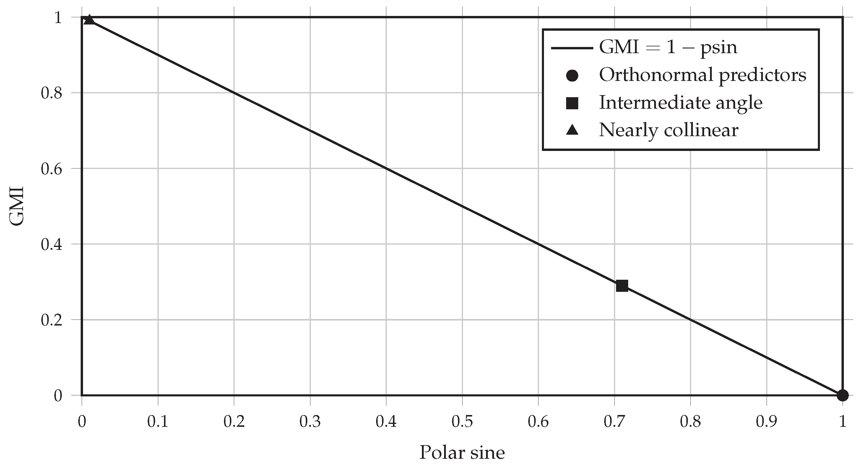
Figure 3.
Two-dimensional schematic of the residual subspace generated by the cross–wedge–QR construction. The vectors and span the predictor space , while and indicate two independent directions in the orthogonal complement prior to QR orthonormalization.
Figure 3.
Two-dimensional schematic of the residual subspace generated by the cross–wedge–QR construction. The vectors and span the predictor space , while and indicate two independent directions in the orthogonal complement prior to QR orthonormalization.
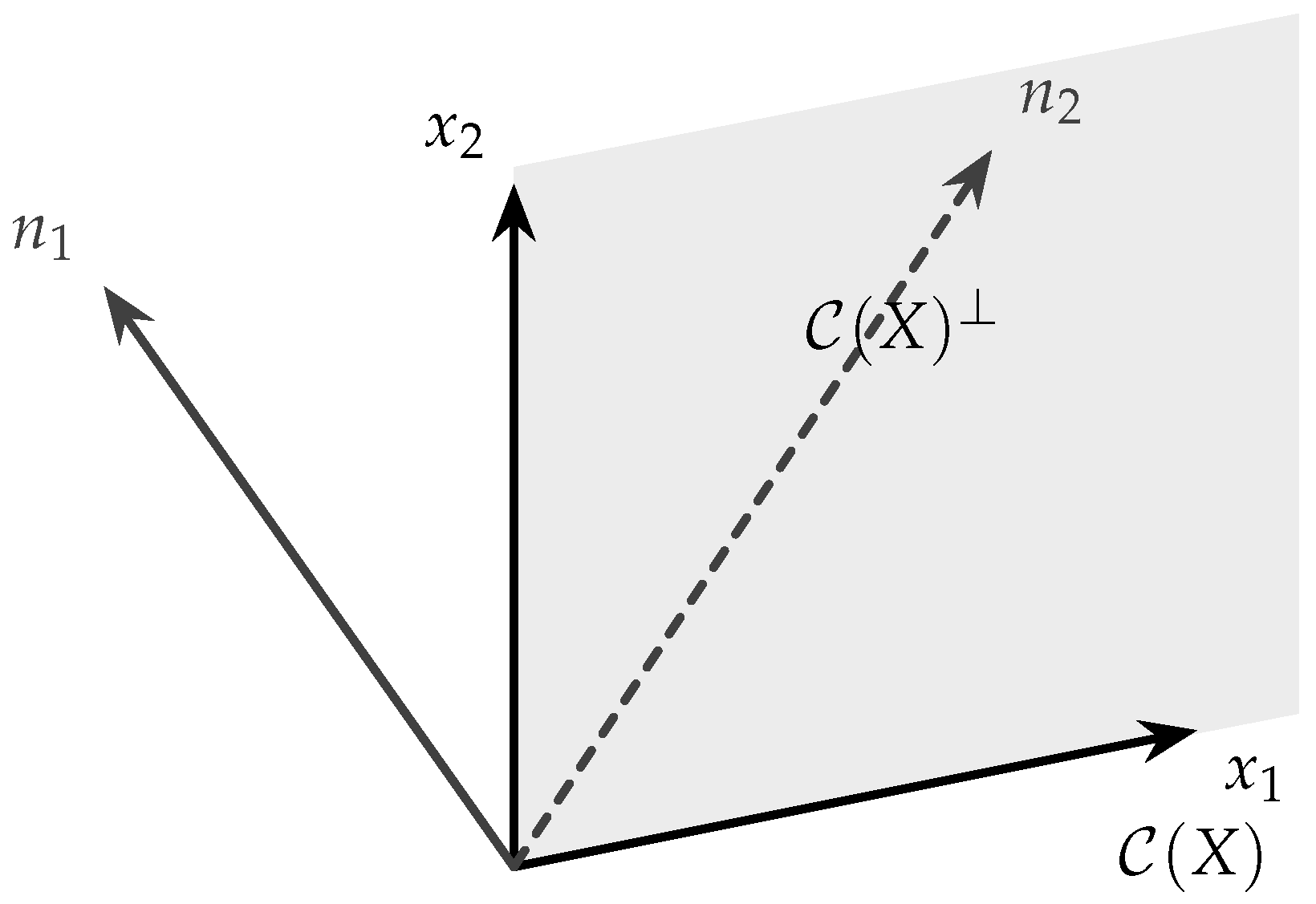
Figure 4.
Residual agreement diagnostics on Boston Housing (standardized). For each model, we plot the pointwise absolute residual discrepancy across observations. Exact projector variants (null-space/QR and, when applicable, Cholesky/OLS) agree with OLS up to numerical precision, while Sketch–QR (Gaussian sketch, ) yields a small but nonzero approximation error. For readability, we visualize discrepancies rather than overlaying multiple residual traces.
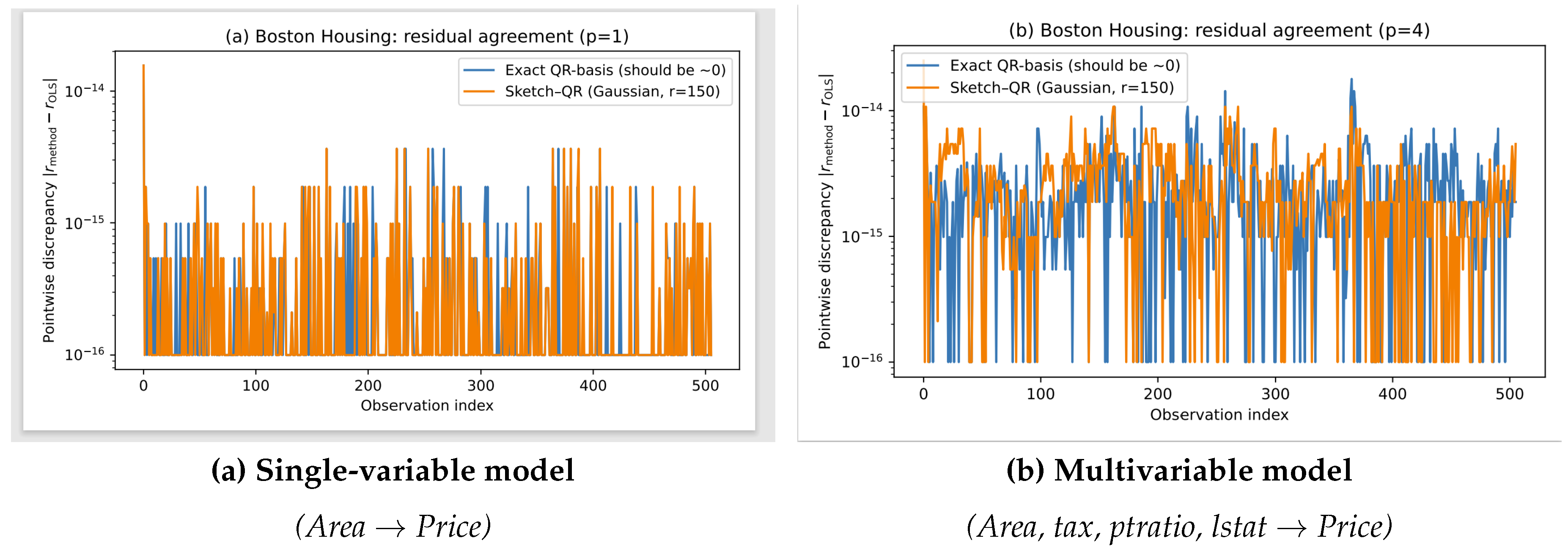

Table 1.
Exact residual projection variants for with rank and residual dimension . The “one-off” cost refers to constructing the projector, while the “per-response” cost refers to applying the residual mapping to a new response vector Y. Methods involving assume that X has full column-rank, so that is invertible.Notes: Classical OLS and the Cholesky-based variant treat the residual subspace implicitly. The QR/null-space basis method also applies to rank-deficient X and explicitly constructs a basis N of . The rank-one cross-product method applies when and is particularly efficient once the normal n is known.
| Method | Residual | One-off cost | Per-response cost |
|---|---|---|---|
| Classical OLS (via ) | |||
| QR / null-space basis | |||
| Cholesky-based (when ) | (form and ) | ||
| Rank-one cross-product () | (construct n) |
Table 2.
Large-scale synthetic multivector residual projection (core methods). The design matrix has , , , and residual codimension . All predictors are standardized. Exact projector variants reproduce the same residual up to numerical precision, while Sketch–QR produces a controlled approximation whose agreement is summarized by cosine similarity. Entries marked as FAIL indicate that the algebraic assumptions of the method (e.g., positive definiteness of for Cholesky-based constructions) are violated, rather than an algorithmic failure.
| # | Method | Runtime (s) | Status | ||
|---|---|---|---|---|---|
| 1 | OLS (Moore–Penrose pseudoinverse) | 0.5092 | 1.000 | 0.0002 | OK |
| 2 | cross-product (rank-one) | NaN | NaN | NaN | N/A |
| 3 | Multivector QR (Exact) | 0.5092 | 1.000 | 0.0000 | OK |
| 4 | Recursive Cross–Wedge–QR | 0.5092 | 1.000 | 0.0008 | OK |
| 5 | Wedge–QR (+GMI) | 0.5092 | 1.000 | 0.0000 | OK |
| 6 | Cholesky–QR | NaN | NaN | 0.0016 | FAIL |
| 7 | Sketch–QR (Gaussian, ) | 0.5092 | 1.000 | 0.0111 | OK |
| Dataset diagnostics: , , . | |||||
Table 3.
Boston Housing illustration (standardized predictors). Predictive metrics are reported using 5-fold cross-validation (CV MSE and CV ). Geometric diagnostics (GMI) are response-independent and depend only on the design matrix X. We additionally report max VIF and , and summarize coefficient stability by under resampling/perturbation, to connect GMI with classical multicollinearity measures.
| Model | p | CV MSE | GMI | max VIF | |||
|---|---|---|---|---|---|---|---|
| (Area/RM → Price/MEDV) | 1 | 44.02 | 0.467 | 0.000 | 1.00 | 1.00 | 0.342 |
| (Area/RM, TAX, PTRATIO, LSTAT) | 4 | 28.02 | 0.655 | 0.434 | 2.09 | 7.85 | 0.257 |
| (Area/RM, LSTAT, PTRATIO, TAX, NOX, INDUS) | 6 | 28.20 | 0.653 | 0.790 | 3.25 | 17.22 | 0.266 |
| Full model (all predictors) | 13 | 23.67 | 0.712 | 0.988 | 9.01 | 96.47 | 0.235 |
Table 4.
Auto MPG illustration (standardized predictors), using the same preprocessing and evaluation protocol as in Section 4.3. Predictive metrics are reported using 5-fold cross-validation (CV MSE and CV ). Geometric diagnostics (GMI) are response-independent and depend only on the design matrix X. We additionally report max VIF and , and summarize coefficient stability by under resampling/perturbation.
| Model | p | CV MSE | GMI | max VIF | |||
|---|---|---|---|---|---|---|---|
| model (Auto) | 1 | 18.91 | 0.682 | 0.000 | 1.00 | 1.00 | 0.118 |
| engine-core (Auto) | 3 | 18.22 | 0.693 | 0.843 | 10.31 | 45.06 | 0.367 |
| model (Auto) | 6 | 12.05 | 0.797 | 0.973 | 19.64 | 117.03 | 0.325 |
| Full model (Auto) | 7 | 11.31 | 0.810 | 0.980 | 21.84 | 136.84 | 0.355 |
Disclaimer/Publisher’s Note: The statements, opinions and data contained in all publications are solely those of the individual author(s) and contributor(s) and not of MDPI and/or the editor(s). MDPI and/or the editor(s) disclaim responsibility for any injury to people or property resulting from any ideas, methods, instructions or products referred to in the content. |
© 2026 by the authors. Licensee MDPI, Basel, Switzerland. This article is an open access article distributed under the terms and conditions of the Creative Commons Attribution (CC BY) license (http://creativecommons.org/licenses/by/4.0/).
Copyright: This open access article is published under a Creative Commons CC BY 4.0 license, which permit the free download, distribution, and reuse, provided that the author and preprint are cited in any reuse.


