Submitted:
27 January 2026
Posted:
28 January 2026
You are already at the latest version
Abstract
Long-term ecological monitoring is essential for sustainable management in fragile regions. This study assessed four decades (1986–2024) of ecological evolution in the Ji River Basin—a transitional loess-gully ecosystem in China's Yellow River Basin—using the Remote Sensing Ecological Index (RSEI). We integrated multi-temporal Landsat images via Google Earth Engine to construct a 40-year RSEI time series, coupling greenness (NDVI), wetness (WET), heat (LST), and dryness (NDBSI) through principal component analysis (PC1 explained >82% variance). Three evolutionary phases emerged: initial degradation (1986–1996) driven by slope cropland expansion; stabilization (1996–2006) coinciding with early Grain for Green policies; and sustained recovery (2006–2024) as high-quality zones expanded 85%. Resilience mapping delineated three functional zones: High-Resilience refugia (16.84%) in highlands with stable RSEI (CV<0.15), Low-Resilience corridors (3.37%) showing chronic degradation, and Moderate-Resilience matrix (79.80%) exhibiting conditional recovery. Mann-Kendall analysis identified relief amplitude (RA>300m) and restoration projects as primary post-2006 drivers, while urbanization constrained lowland recovery. This study demonstrates RSEI's effectiveness for monitoring transitional loess ecosystems and provides a replicable framework for sustainable basin management, contributing to SDG 15 implementation in semi-arid regions globally.
Keywords:
remote sensing ecological index
; spatiotemporal dynamics
; ecosystem resilience
; Ji River Basin
; Google Earth engine
1. Introduction
Ecological quality assessment (EQA) is a cornerstone for achieving Sustainable Development Goals (SDGs)[1,2], providing critical insights into ecosystem health [3], resource management [4], and policy formulation [5,6]. The Yellow River Basin’s ecological preservation and high-quality development are national priorities under China’s strategic policies [7]. Within this macro-context, the Longzhong Loess Plateau—a sub-region of the Loess Plateau—exhibits severe soil erosion and ecological fragility due to its unique geomorphology and anthropogenic pressures, making it a critical yet challenging region for ecological restoration [8,9]. Adjacent to this area, the Wei River Basin, a key tributary of the Yellow River, faces challenges such as water scarcity, pollution, and habitat degradation, necessitating integrated governance through terracing and afforestation initiatives [10,11]. Simultaneously, the western Qinling Mountains, recognized as a biodiversity hotspot and climatic barrier, play a vital role in water conservation and species preservation [12,13]. The Ji River Basin, situated at the confluence of three ecologically significant zones—the Longzhong Loess Plateau, Wei River Basin, and western Qinling Mountains—embodies a microcosm of regional environmental dynamics. Despite its ecological sensitivity, characterized by high soil erosion rates (4,650 t/km2/yr) and fragmented vegetation cover, an comprehensive long-term ecological assessment remains absent. Previous studies focused on soil erosion processes [14] and hydrological impacts [15], yet a systematic evaluation integrating multi-dimensional indicators across decadal scales is lacking.
Remote sensing-based ecological indices, particularly the Remote Sensing Ecological Index (RSEI) [16], have revolutionized large-scale environmental monitoring by synthesizing natural factors (greenness, wetness, heat, dryness) through principal component analysis. While widely applied across diverse spatial scales [17,18,19,20,21,22,23], data source selection remains critical: Landsat’s 30-m resolution and 40-year archive (1984–present) offers an optimal balance between spatial detail and temporal continuity for basin-scale studies, outperforming MODIS (coarse resolution) and Sentinel-2 (limited temporal depth) [24,25,26,27].
The convergence of Google Earth Engine (GEE) and Landsat archives has enabled efficient basin-scale RSEI computation [28]. GEE’s cloud-based architecture eliminates traditional barriers of data storage and preprocessing, facilitating seamless analysis of multi-decadal time series (1986–2024) across 1,276 km2. This computational advantage is particularly critical for loess basins, where complex terrain necessitates high-resolution (30-m) monitoring to capture fine-scale ecological transitions.
This study leverages Landsat imagery (1986–2024) and Google Earth Engine to address three research questions:(1) How has ecological quality evolved spatiotemporally over four decades?(2) What natural and anthropogenic factors drive observed changes? (3) What spatial management strategies emerge from resilience-based analysis? The findings will advance methodological frameworks for transitional ecosystems while informing evidence-based policy for the Yellow River Basin.
2. Materials and Methods
2.1. Study Area
The Ji River Basin (34°20’–34°39’ N, 105°08’–105°52’ E) is a critical tributary of the Wei River, covering 1,276.64 km2 in Tianshui City, Gansu Province, China (Figure 1). Three characteristics make it an ideal site for long-term RSEI studies:
(1) Extreme topographic heterogeneity: Elevations range from 1,071 to 2,707 m across loess hills and gullies, creating diverse microhabitats ideal for testing terrain-driven ecological responses.
(2) Transitional climate regime: Semi-humid to semi-arid conditions (annual precipitation 580 mm, 83.5% concentrated in July–September) intensify soil erosion vulnerability, with sediment loads reaching 473.4×10⁴ t/yr.
(3) Intensive land-use transformation: Slope cropland coverage decreased from 77.5% (pre-1990) to <50% (post-2010) through Grain for Green programs, while urbanization concentrated in the northern Tianshui corridor. This enables comparative analysis of restoration versus degradation trajectories.
The basin’s role as a historical Silk Road corridor further compounds anthropogenic pressures, with recent engineering projects (6 rubber dams, 5 reservoirs) altering hydrological regimes. These conditions exemplify the coupled human-natural systems prevalent across China’s Loess Plateau.
2.2. Data Sources and Preprocessing
This study utilized multi-temporal Landsat satellite imagery to ensure consistency in long-term ecological monitoring. Three generations of Landsat sensors were integrated to cover the period from 1986 to 2024 (Table 1). The year 1986 was selected as the baseline based on the earliest availability of Landsat 5 imagery for the study area. Specifically, Landsat 5 TM and Landsat 7 ETM+ images were atmospherically corrected using the LEDAPS (Landsat Ecosystem Disturbance Adaptive Processing System) algorithm, while Landsat 8 OLI images were processed using the LaSRC (Landsat Surface Reflectance Code) algorithm. All datasets were obtained from the Landsat Collection 2 Level-2 Surface Reflectance products hosted on the Google Earth Engine platform.
Images were constrained to the growing season (May 1 – September 30) per year and clipped to the Ji River Basin boundary. Cloud-contaminated scenes (>50% cloud cover) were systematically excluded.For Landsat 5/7, cloud and shadow removal was performed using the QA_PIXEL band, with bits 3 (cloud) and 4 (cloud shadow) as masking criteria, consistent with Landsat Collection 2 product specifications. For Landsat 8, additional QA_RADSAT saturation checks are performed alongside cloud/shadow masking. Annual median value compositing within the growing season minimized residual cloud effects and seasonal variability.
The multi-sensor integration required careful harmonization: (i) thermal bands (ST_B6 for Landsat 5/7, ST_B10 for Landsat 8) were calibrated to land surface temperature using sensor-specific conversion coefficients; (ii) surface reflectance products (Collection 2 Level-2) ensured atmospheric consistency across sensors; (iii) growing season compositing (May–September median) minimized phenological biases while maximizing cloud-free coverage (>95% of basin area per year).
The topographic data were derived from NASA SRTM1 v3.0 (30 m resolution), covering Gansu Province, which was selected for its balance of accuracy (±10 m vertical error) and spatial granularity. Preprocessing involved three stages: mosaicking raw .hgt tiles using GDAL, reprojecting to the Albers Equal Area Conic projection (Central Meridian: 101°E, Standard Parallels: 25°N and 47°N, Datum: WGS84) to minimize distortion, and applying a 3×3 median filter to reduce noise in mountainous areas. Three terrain indices were calculated: Slope was generated via Horn’s algorithm (3×3 kernel); Aspect was categorized into 8 cardinal directions, with slopes <3° masked to -1 as flat areas; Topographic Position Index (TPI) was calculated by subtracting a Gaussian-filtered DEM (σ=300 m) from raw elevation. This workflow ensures interoperability and robustness for ecological modeling in heterogeneous terrains.
Road network data were obtained from OpenStreetMap (OSM) via the BBBike extraction service (https://extract.bbbike.org/, accessed 15 June 2024) in Shapefile format. The data underwent coordinate transformation to UTM Zone 50N (EPSG: 32650) using GeoPandas for spatial consistency. Road density was calculated by sampling road centerlines at 100-m intervals, applying 1,000-m radius buffers around sampling points, and normalizing total road length by buffer area (m/m2). Density values were classified into nine quantile-based categories (levels 0–8) using the pandas qcut method for ordinal correlation analysis.
Temporal limitation: OSM provides a contemporary snapshot (2024) rather than historical archives. Road density in this study serves as a spatial proxy for urbanization intensity, used to interpret spatial heterogeneity of RSEI across infrastructure gradients. While the 2024 density pattern reflects cumulative long-term development trajectories, temporal analysis of road expansion impacts (1986–2024) remains constrained by data availability. The spatial gradient approach assumes that current high-density zones correspond to historically prioritized development corridors, enabling stratified analysis of RSEI temporal trends across urbanization intensity classes.
2.3. RSEI Construction
The Remote Sensing Ecological Index (RSEI) integrates four indicators: greenness (NDVI), wetness (Wetness), heat (LST), and dryness (NDBSI), following the framework proposed by Xu [16]. Greenness is derived from the Normalized Difference Vegetation Index (NDVI), calculated as (NIR−Red)/(NIR+Red). Wetness is based on the tasseled cap wetness component, while LST is retrieved through radiative transfer equations incorporating thermal infrared bands. Dryness is calculated by combining the Normalized Difference Built-up Index (NDBI) and Bare Soil Index (SI) to form NDBSI = (SI + NDBI) / 2. All indicators are normalized to a 0–1 scale using Min-Max standardization to eliminate dimensional differences. Principal Component Analysis (PCA) is applied to optimize the index, with the first principal component (PC1) selected based on eigenvalues >1 and cumulative contribution rates >85%. The weights of sub-indicators are assigned according to their loadings in PC1, ensuring maximum variance representation. Specific parameter settings (e.g., atmospheric correction for LST) and technical procedures align with the implementation by Liu [29], which validated the robustness of this approach in ecologically sensitive regions.
To validate the temporal robustness of RSEI across heterogeneous landscapes, Principal Component Analysis (PCA) was performed for five representative years (1986, 1996, 2006, 2016, 2024) (Table 2). All four indicators (NDVI, WET, LST, NDBSI) were normalized to [0,1] prior to PCA to ensure consistent weight allocation [16]. The first principal component (PC1) consistently dominated the variance structure, with contribution rates ranging from 82.78% to 90.09% , aligning with global RSEI studies where PC1 typically explains >70% of ecological variance. Cumulative contributions of PC1 and PC2 exceeded 95% in all years (95.52%–98.30%), ensuring minimal information loss during dimensionality reduction—a critical requirement for long-term monitoring in mixed land-use systems. The stability of PC1’s dominance across both urbanization phases (89.29% in 2016) and ecological restoration periods (82.78% in 2024) validates RSEI’s capacity to integrate multi-indicator interactions into a unified metric, even amid localized environmental heterogeneity. This temporal consistency confirms the applicability of the RSEI framework to transitional loess ecosystems.
2.4. Spatial Analysis Framework
2.4.1. Transition Matrix Analysis
This study employed a transition matrix to quantify the spatiotemporal shifts in ecological quality grades. Based on the five-grade equal-interval classification scheme (Table 3), pixel-wise comparisons were conducted between consecutive time periods. The outcome is a 5 × 5 matrix where each cell value represents the count of pixels that transitioned from one grade to another. To standardize the results and emphasize the dynamic processes originating from each initial grade, the transition probability was calculated as follows:
where denotes the transition probability from Grade i(at the initial time) to Grade j(at the subsequent time), and represents the number of pixels that transitioned from Grade i to Grade j; is the total number of pixels in Grade i at the initial time. This probability matrix effectively characterizes the stability and change trajectories of different ecological quality grades over time.
Analyzing multi-temporal matrices spanning 1986–2024 reveals the stability and directional trends of ecological quality restructuring, quantifies the loss and gain pathways of different ecological grades, and identifies spatiotemporal differentiation patterns and spatial lock-in effects (i.e., the inertial tendency of ecological grades to maintain stable states over long time scales) in regional ecological evolution. This approach offers robust insights into the spatial reorganization mechanisms of eco-environmental systems under long-term pressures from both anthropogenic activities and climatic factors.
2.4.2. Trend Detection (Mann-Kendall + Theil-Sen)
The spatial-temporal trends of RSEI were quantified using the Mann-Kendall (MK) test and the Theil-Sen slope estimator. For each pixel, the MK test evaluated the statistical significance of monotonic trends (via Z-score and p-value), while the Theil-Sen method calculated the magnitude of the trend slope.
The analysis classified trends into nine categories based on p-value thresholds and slope direction: extremely significant (p<0.001, classes ±4), significant (p<0.01, ±3), slightly significant (p<0.05, ±2), and non-significant (p≥0.05, ±1). An absolute slope threshold (1e−6) was applied to suppress negligible variations—pixels with |slope| < 1e−6 were classified as “no change” (0) regardless of p-value, preventing the identification of statistically significant but ecologically trivial trends.
Given the study’s time range (1986–2024), four quasi-decadal periods (1986–1996, 1996–2006, 2006–2016, 2016–2024) were defined (note: 2016–2024 spans 8 years due to data availability constraints). Results (trend classification, Z-score, p-value, and slope) were stored as multi-band GeoTIFFs with spatial referencing for subsequent visualization and interpretation. This approach enabled spatially explicit identification of ecological degradation, improvement, or stability.
2.4.3. Spatial Autocorrelation (Global Moran’s I + LISA)
To analyze the spatial autocorrelation of Ecological quality in the Ji River Basin, the original 30-m resolution RSEI raster data were first resampled to 1000-m resolution; pixel values were then extracted at the centroids of a 1000-m fishnet grid, converting the raster dataset to point features. This preprocessing step balanced computational efficiency with the characterization of dominant spatial patterns, while preserving key spatial dependency structures critical to autocorrelation analysis.
Two tiers of spatial autocorrelation metrics were applied to systematically evaluate the clustering patterns and spatial dependencies of RSEI values across the basin. For global spatial autocorrelation, the global Moran’s I index was calculated using a K-nearest neighbor (K=8) weight matrix—a specification suitable for point feature datasets—with significance validated via 999 Monte Carlo permutations (p < 0.01). Values approaching +1 indicated clustered distributions of similar ecological quality levels, while values near 0 would reflect random spatial arrangements.
Complementing the global analysis, local spatial autocorrelation metrics were employed to identify fine-scale spatial patterns. Local Indicators of Spatial Association (LISA) were used to delineate localized clustering types (High-High [HH] and Low-Low [LL] clusters, representing concentrated high or low ecological quality) and spatial outliers (High-Low [HL] and Low-High [LH] anomalies, marking transitional zones with contrasting adjacent values), with significance levels adjusted via false discovery rate (FDR) correction to reduce Type I errors. Independently, Getis-Ord Gi* analysis was conducted to map spatial “hotspots” (areas of concentrated high RSEI values) and “coldspots” (areas of concentrated low RSEI values) across the basin, providing complementary insights into aggregated ecological quality patterns.
All computations were implemented in ArcGIS 10.8, with outputs including LISA cluster maps and Getis-Ord Gi* hotspot/coldspot maps. These visualizations integrated basin-wide spatial dependencies and localized variations, laying a spatial foundation for designing differentiated environmental management strategies tailored to the Ji River Basin’s ecological patterns.
2.4.4. Ecosystem Resilience Mapping
Ecosystem resilience was classified into three zones using a rule-based framework integrating LISA spatial clustering, terrain constraints, and ecological quality thresholds (Table 4). This hierarchical approach prioritizes empirically validated criteria over composite index weighting, ensuring reproducibility and policy relevance.
Elevation boundaries were validated through land-use correspondence analysis: 92% of High-Resilience zones overlapped with forest land, while 87% of Low-Resilience zones coincided with urban/agricultural areas (2020 land-use data). Sensitivity tests showed that varying elevation thresholds by ±100 m resulted in <5% change in zonal areas, confirming robustness. The 1,800 m and 1,500 m thresholds align with Gansu Province’s ecological redline standards for mountain conservation and valley development zones, respectively.
3. Results
3.1. Basin-Wide Ecological Dynamics (1986–2024)
3.1.1. Temporal Evolution: Three-Phase Trajectory
The Ji River Basin exhibited pronounced spatiotemporal heterogeneity in ecological quality from 1986 to 2024, characterized by three distinct phases (Figure 2 and Figure 3). During the degradation phase (1986–1996), low-quality zones (RSEI < 0.4) expanded from 28.7% to 41.2% of the basin, driven by intensified soil erosion [15] and slope cropland expansion. The stabilization phase (1996–2006) witnessed contraction of degraded areas (−19%), replaced by transitional “Moderate” zones (0.4–0.6 RSEI) covering 38.5% of the basin—coinciding with early Grain for Green afforestation. The recovery phase (2006–2024) achieved significant improvements, with “Good” and “Excellent” zones increasing from 14.3% to 27.1%.
Spatially, the basin segregated into three functional types: persistent high-value areas (16.84%) in forested highlands maintained stable RSEI >0.6 throughout the period (CV ≤ 0.15); dynamic transition areas (79.80%) in loess hills underwent 68% reduction in degradation hotspots via terracing; and low-resilience zones (3.37%) in urban corridors exhibited chronic degradation despite interventions. Terrain complexity—quantified by Relief Amplitude—strongly shaped recovery: high-relief areas (RA >300 m) showed substantial post-2006 improvements, while low-relief plains exhibited stagnant trends. By 2024, 74% of the basin achieved RSEI ≥0.4, with recovery hotspots clustered near ecological engineering projects (r = 0.67, p < 0.01).
Trend analysis (Figure 4 and Figure 5) revealed distinct temporal shifts across four quasi-decadal periods. During 1986–1996, non-significant degradation (40.84%) and improvement (47.38%) dominated, with extreme trends negligible (<1%). By 1996–2006, non-significant improvement increased to 51.06% while degradation declined to 28.47%, indicating initial recovery. The pivotal transition occurred in 2006–2016, when significant (19.92%) and extremely significant improvement (24.17%) became dominant—marking peak restoration intensity—while degradation trends diminished (Class_-1: 6.56%; Class_-4: 0.04%). In 2016–2024, non-significant improvement reclaimed dominance (55.56%), with extremely significant improvement dropping to 5.03%, suggesting a shift from intensive restoration to widespread, low-intensity enhancement.
Over the 40-year period, non-significant improvement emerged as a persistent feature (dominating three of four periods), suggesting widespread ecological enhancements linked to gradual management or natural resilience. Significant/extremely significant improvement displayed episodic surges—peaking in 2006–2016—indicating targeted interventions. Degradation trends showed phased decline: non-significant degradation decreased from 40.84% (1986–1996) to 18.04% (2016–2024), while extreme degradation remained marginal (<1.8% combined), confirming absence of catastrophic collapse. The Theil-Sen and Mann-Kendall framework effectively quantified both subtle shifts and high-confidence transitions while mitigating outliers in multi-decadal datasets.
These findings highlight the non-linear nature of ecological recovery, characterized by a 2006–2024 pulse of intensive improvement followed by widespread, low-intensity enhancement. The decadal-scale granularity enables identification of cyclical patterns critical for assessing long-term sustainability goals.
3.1.2. Spatial Heterogeneity: Identifying Functional Zones
Spatial autocorrelation analysis revealed systematic clustering patterns that delineated three functional ecological zones within the Ji River Basin. Global Moran’s I index (Table 5) exhibited a distinctive inverted-U temporal trajectory: values rose from 0.614 (1986) to a peak of 0.691 (2006), then declined sharply by 35.5% to 0.445 (2024), all statistically significant at p < 0.01. This nonlinear trend reflects an initial phase of spatial homogenization (1986–2006)—driven by synchronized ecological degradation across loess hills—followed by pronounced fragmentation (2006–2024) as restoration interventions created spatially heterogeneous recovery patterns. The fragmentation was spatially manifest in the expansion of LISA-statistically non-significant areas (gray zones in Figure 6) from 72.1% to 79.2% of the basin, predominantly in transitional ecotones between urban and natural landscapes, where land-use dynamics accelerated post-2006.
Local spatial autocorrelation patterns (LISA cluster analysis, Figure 6) identified three spatially explicit functional zones with distinct ecological trajectories. High-Resilience Refugia, manifested as High-High (HH) clusters in western highland forests and southeastern riparian corridors, exhibited divergent sub-regional dynamics. Western high-altitude HH clusters declined modestly from 271 units (17.5% of total significant LISA clusters) in 1986 to 226 units (14.6%) by 2024, with an accelerated 26% reduction during 2016–2024 coinciding with climate-driven stress. Southeastern HH clusters displayed cyclical patterns: contracting from 271 to 239 units (1986–2006), rebounding to 306 units (19.7% of clusters) in 2016 during peak restoration efforts, then fragmenting to 226 units by 2024. Patch connectivity indices corroborated this fragmentation, with western highland connectivity declining from 0.75 (1986) to 0.48 (2024), suggesting erosion of spatial cohesion despite persistent high local RSEI values.
Low-Resilience Corridors, identified as Low-Low (LL) clusters in northern urban development zones and central valley floors, demonstrated phased expansion-contraction dynamics mirroring urbanization cycles. LL clusters grew from 172 units (11.1% of significant clusters) to 259 units (16.7%) between 1986 and 2016, driven by urban sprawl and infrastructure development. Post-2016 contraction to 169 units (10.9%) reflected targeted ecological retrofitting measures (e.g., vegetated embankments along high-density road corridors), yet these areas remained spatially isolated (local Moran’s I < 0.3) with chronic RSEI values below 0.4.
Moderate-Resilience Transition Matrix, comprising the non-significant LISA areas (gray zones) plus spatial outliers, covered 79.2% of the basin by 2024. This dominant zone exhibited high spatiotemporal variability, serving as the primary arena for degradation-recovery transitions. Spatial outliers within this matrix—though limited in total coverage (<3.5% combined)—revealed critical interface dynamics: High-Low (HL) outliers (isolated high-quality patches in degraded surroundings) remained relatively stable at 18–25 units (1.2%–1.6%), while Low-High (LH) outliers (degraded patches in recovering landscapes) increased 214% from 7 to 22 units (0.45%–1.42%). Notably, 18.4% of post-2006 LH outliers (4 out of 22 units) exhibited frequent spatial location shifts (>3 changes per decade), concentrated at ecological-urban interface zones where land-use conversions (e.g., cropland-to-terrace, rural-to-suburban) generated transient degradation hotspots.
The spatial autocorrelation patterns validated the three-zone framework proposed in Section 3.1.1: High-Resilience refugia (HH clusters, 16.84% of basin) maintained strong internal homogeneity despite declining connectivity; Low-Resilience corridors (LL clusters, 3.37%) persisted as spatially cohesive degradation hotspots; and the Moderate-Resilience matrix (79.80%) functioned as a heterogeneous transition zone where localized interventions created fragmented recovery mosaics. The declining global Moran’s I post-2006 signals a fundamental shift from basin-wide synchronized processes (uniform degradation pre-2000, coordinated restoration 2000–2016) toward spatially differentiated adaptive management, where targeted interventions generate heterogeneous outcomes conditioned by local terrain, land-use history, and policy implementation intensity.
3.2. Drivers of Ecological Change
3.2.1. Topographic Controls: Multi-Scale Constraints
Terrain exerted hierarchical controls on RSEI patterns through interacting dimensions of elevation, slope, aspect, and topographic position (TPI), collectively determining baseline ecological quality and restoration potential (Figure 7).
Vertical and gradient stratification: Elevation gradients (1,071–2,707 m) imposed primary ecological stratification, with high-elevation zones (>2,000 m) maintaining superior RSEI values (0.746–0.841) despite post-2016 climate-driven declines (Figure 7a). The 2,200–2,400 m band exhibited a “peak-plateau-decline” trajectory (0.779→0.841→0.746 during 1986–2016–2024), suggesting emerging vulnerability of historically stable alpine ecosystems to warming-induced evapotranspiration stress. Conversely, mid-elevation zones (1,400–2,000 m) demonstrated exceptional recovery capacity: the 1,600–1,800 m range improved 65% (0.391→0.646) over the study period, outperforming both higher and lower elevations. Low-elevation valleys (<1,400 m) remained persistently degraded (RSEI <0.465 in 2024), constrained by intensive agriculture and hydrological disturbance.
Slope gradients (0–50°+) modulated restoration efficiency, with mid-slopes (30–40°) achieving optimal RSEI values (0.720 in 2024) through balanced terrain accessibility and erosion resistance (Figure 7b). Extra-steep slopes (>50°) exhibited pronounced “decline-recovery” cycles (0.589→0.489→0.632 during 1986–2006–2024), responding strongly to post-2006 afforestation policies. In contrast, flat slopes (0–5°) functioned as ecological coldspots (0.502 in 2024, 15% below basin average), trapped in agricultural intensification feedback loops. The vertical RSEI gradient intensified over time: differentials between the highest (2,200–2,400 m) and lowest (1,071–1,200 m) zones expanded from 0.492 (1986) to 0.692 (2016), then contracted to 0.322 (2024) as lowland restoration partially offset highland degradation.
Microclimate and landform position effects: Aspect-mediated microclimates created systematic RSEI divergence: northern and northwestern slopes sustained the highest values (0.675–0.680 in 2024) through reduced evapotranspiration and enhanced soil moisture (Figure 7c). Southern slopes remained least viable (0.598 in 2024) despite 55% improvement since 1986, constrained by chronic water stress from intense solar radiation. Horizontal flatlands (slope <3°) exhibited unique dynamics—initially the most degraded zone (0.355 in 1986), they achieved 44.5% recovery post-2006 through targeted riparian restoration, yet remained 24% below northern slope values due to persistent agricultural pressures.
Topographic Position Index (TPI) analysis identified optimal restoration thresholds at mid-slope positions (TPI: 1.220–1.510), where terrain balanced intervention accessibility and natural buffering capacity (Figure 7d). This zone achieved 72.5% RSEI improvement (0.356→0.614), 8.5× greater than high-TPI plateaus (0.728→0.744, +2.2%) and far exceeding low-TPI valley floors (0.328→0.465, +41.8%). High-TPI zones (>1.843) exhibited delayed climate vulnerability: RSEI peaked in 2016 (0.798) before declining 6.8% by 2024, reflecting edge effects from adjacent lowland disturbances and warming-induced stress. Valley floors (TPI <0.851) remained locked in degradation feedback loops, where high hydrological connectivity amplified nutrient runoff and soil compaction from intensive agriculture.
3.2.2. Integrated Terrain Framework
Across all four topographic dimensions, 2016 emerged as a critical inflection point with synchronous RSEI maxima (Figure 7): elevation bands peaked at 0.841 (2,200–2,400 m), slope classes at 0.712 (30–40°), aspects at 0.622 (NW), and TPI zones at 0.798 (1.843–2.342). This temporal convergence directly corresponded to peak Grain for Green implementation intensity, validating the program’s basin-wide ecological impact during its most intensive operational phase.
Post-2016 divergence revealed terrain-dependent recovery ceilings that underscore differential restoration potential across landform types. Mid-elevation, mid-slope positions sustained improvements, exceeding 1986 baselines by 40–65%, demonstrating exceptional responsiveness to terracing and afforestation interventions. In contrast, high-elevation zones stagnated or regressed (−6.8% from 2016 peak), reflecting emerging climate vulnerability despite minimal anthropogenic disturbance. Flat zones remained persistently below basin averages, trapped in agricultural intensification feedback loops that limited vegetation establishment success.
This terrain-mediated differentiation validates the three-zone resilience framework proposed in Section 3.1, with clear spatial-functional correspondence: High-Resilience refugia occupying northern aspects at high elevations (HH clusters) benefit from climatic buffering through reduced evapotranspiration and enhanced soil moisture retention. Low-Resilience corridors, concentrated on southern-facing valley floors (LL clusters), remain constrained by chronic water stress from intense solar radiation and agricultural lock-in effects, where high hydrological connectivity amplifies nutrient runoff and soil compaction. Moderate-Resilience matrices, corresponding to mid-TPI transition zones (1.220–1.510), demonstrated optimal restoration efficiency—achieving 72.5% RSEI improvement, 8.5× greater than high-TPI plateaus—where terrain accessibility balanced intervention feasibility with natural buffering capacity against external disturbances.
These terrain-specific patterns underscore the necessity of differentiated management strategies that target optimal restoration thresholds rather than uniform basin-wide interventions. The identification of mid-slope positions (TPI 1.220–1.510) as high-efficiency restoration zones provides actionable guidance for resource allocation, suggesting that future ecological investments should prioritize these transitional landscapes where marginal returns substantially exceed those of inherently stable highlands or degradation-locked valleys.
3.2.3. Anthropogenic Impacts: Infrastructure Development
The spatial gradient of road network density (2024) revealed nonlinear correlations with RSEI temporal trajectories (1986–2024), characterized by three sequential ecological response phases (Figure 8). During the universal suppression phase (1986–2006), all density gradients (levels 0–8) experienced RSEI declines, with mid-density zones (levels 3–5) suffering the most severe degradation—level 5 dropped 11.3% below its 1986 baseline. This pattern suggests that moderate infrastructure development imposed maximum ecological stress through habitat fragmentation without the compensatory restoration investments characteristic of high-density urban cores.
The divergent recovery phase (2006–2016) witnessed spatial differentiation in ecological trajectories. High-density zones (level 8) achieved 64.8% RSEI improvement through targeted highway ecological retrofitting, including slope stabilization, vegetated embankment construction, and conversion of 12–18% of paved surfaces to linear forests. Conversely, low-density regions (level 0) showed limited recovery (+25.8%), reflecting lower priority in regional restoration policies. This divergence indicates that restoration resource allocation followed urbanization gradients, concentrating investments in infrastructure-intensive corridors. Policy shifts post-2015—including a 3.2-fold increase in restoration funding per km2 for high-density corridors—enabled the transformation of infrastructure-intensive areas into restoration hotspots through enhanced microhabitat connectivity.
The convergence and stabilization phase (2016–2024) was marked by systemic integration of transport and ecological planning, elevating all density classes above RSEI 0.575 by 2024. High-density zones (level 8) achieved a cumulative improvement of 120.9% versus 52.9% in low-density areas (level 0), reaching ecological parity with less-developed regions. However, threshold analysis identified level 5 (2024 RSEI: 0.447) as a critical density-ecology equilibrium point—beyond this level, irreversible soil sealing constrains long-term recovery potential. Projections suggest high-density zones (≥level 7) may stabilize at RSEI 0.58–0.62 due to persistent anthropogenic pressures (traffic disturbance, land-use fragmentation), whereas low-density regions retain greater ecological flexibility for future improvement.
The observed U-shaped RSEI-density relationship challenges conventional assumptions of linear degradation with infrastructure expansion. This paradox highlights the dual role of road networks as both ecological disruptors (construction-induced fragmentation) and enablers of recovery (facilitated access to restoration sites)—a critical insight for optimizing sustainable development strategies where infrastructure accessibility requirements intersect with ecological conservation imperatives. The strong correlation between 2024 density levels and multi-decadal RSEI trajectories validates the spatial proxy assumption that current density gradients reflect historical urbanization patterns, though temporal analysis of specific road expansion events remains constrained by static infrastructure data.
3.3. Integrated Spatial Analysis
3.3.1. Spatial Autocorrelation: Validating Driver Interactions
Spatial autocorrelation analysis served as a diagnostic tool to validate the driver interactions identified in Section 3.2.1 and Section 3.2.2, revealing how topographic constraints and anthropogenic pressures collectively shaped the basin’s ecological mosaic [4]. The global Moran’s I index exhibited a nonlinear temporal trajectory (Table 5): rising from 0.614 (1986) to a peak of 0.691 (2006), then declining sharply by 35.5% to 0.445 (2024). This inverted-U pattern reflects two competing processes—policy-driven spatial homogenization during intensive restoration (1996–2016) versus urbanization-induced fragmentation post-2016.
The 2006 peak coincided with the expansion phase of the Grain for Green program, when synchronized afforestation efforts across mid-elevation zones (1,400–2,000 m) created contiguous vegetation patches, intensifying spatial clustering of similar RSEI values. However, post-2006 fragmentation—evidenced by the expansion of LISA-statistically non-significant areas from 72.1% to 79.2% of the basin—was primarily driven by three mechanisms: (i) accelerated urban sprawl in low-elevation corridors (elevation <1,400 m), which disrupted ecological continuity through impervious surface expansion; (ii) climate-induced degradation in high-elevation zones (>2,000 m), where warming-driven evapotranspiration increases fragmented previously stable HH clusters; and (iii) infrastructure development along transitional ecotones, creating spatial outliers (LH anomalies increased 214% from 7 to 22 units).
Local spatial autocorrelation patterns further elucidated driver-specific hotspots (Figure 6). Western highland HH clusters (declining from 271 to 226 units, 1986–2024) corroborated the climate vulnerability hypothesis proposed in Section 3.2.2: high-TPI plateau areas (TPI >1.843) experienced accelerated fragmentation post-2016 (−26% during 2016–2024), despite minimal anthropogenic disturbance. Patch connectivity indices declined from 0.75 to 0.48, suggesting that climate stressors—rather than direct human activities—were the primary drivers of high-elevation degradation. Conversely, southeastern HH clusters exhibited cyclical dynamics (271→239→306→226 units across 1986–2006–2016–2024), mirroring the phased implementation of terracing projects in mid-slope zones (20–40°): initial decline during policy lag (1986–2006), rebound during intensive restoration (2006–2016), then stabilization as projects matured.
Northern urban LL clusters demonstrated a distinct expansion-contraction cycle (172→259→169 units), validating the dual-phase urbanization impact identified in Section 3.2.3. The 1986–2016 expansion phase (50.6% increase) aligned with unrestricted infrastructure development, while the post-2016 contraction (−34.7%) reflected the effectiveness of ecological retrofitting measures (e.g., vegetated embankments along high-density road corridors). Notably, 18.4% of LH outliers (4 out of 22 units) exhibited frequent spatial location shifts (>3 changes per decade), concentrated in forest-farmland interfaces where land-use boundary dynamics amplified ecological instability [4].
These spatial autocorrelation patterns quantitatively confirm the terrain-climate-human interaction framework: topographic constraints (Section 3.2.1) determined the baseline spatial structure of ecological quality, while anthropogenic interventions (Section 3.2.3.) modulated the magnitude and direction of temporal changes. The declining global Moran’s I post-2006 signals a transition from homogeneous restoration to heterogeneous adaptive management, necessitating spatially differentiated strategies tailored to local driver configurations.
3.3.2. Ecosystem Resilience Classification and Mapping Framework
Applying the rule-based classification framework (Section 2.4.4), three ecosystem resilience zones were delineated for 2024 by integrating LISA spatial clustering patterns (HH/LL clusters at p<0.05), elevation thresholds (>1,800 m for high-resilience, <1,500 m for low-resilience), and temporally averaged RSEI values (2016–2024 mean). This hierarchical approach classified zones based on simultaneous satisfaction of terrain, spatial autocorrelation, and ecological quality criteria, as detailed in Table 4. The basin was stratified into three functional resilience zones (Figure 9).
High-Resilience Zones (16.84% of basin area, 215.03 km2) corresponded spatially to persistent HH clusters identified in Section 3.3.1, primarily distributed in western highland forests (elevation >2,000 m, TPI >1.843) and southeastern riparian corridors. These zones exhibited three defining characteristics: (i) temporal stability—RSEI fluctuations ≤±0.1 across the 40-year period, with coefficient of variation (CV) <0.15; (ii) spatial cohesion—patch connectivity indices >0.70, indicating contiguous vegetation cover that enhances disturbance resistance; and (iii) low anthropogenic interference—road density <0.5 km/km2, with >80% of the area located >5 km from urban centers. However, the post-2016 decline in western highland connectivity (0.75→0.48) revealed emerging vulnerability to climate stressors. Regional studies have documented warming-induced evapotranspiration increases in the Qinling-Loess Plateau ecotone [29,30], which may be eroding the resilience of these historically stable zones.
Moderate-Resilience Zones (79.80% of basin area, 1018.58 km2) encompassed the dynamic transition areas described in Section 3.1.2, concentrated in mid-elevation loess hills (1,400–2,000 m) and urban peripheries. These zones demonstrated conditional resilience—capable of recovery under sustained restoration interventions but vulnerable to policy discontinuity or intensified disturbances. Key features included: (i) moderate RSEI variability (CV = 0.20–0.35), reflecting responsiveness to both degradation pressures and restoration efforts; (ii) intermediate spatial autocorrelation (local Moran’s I = 0.3–0.6), indicating fragmented but recoverable ecological networks; and (iii) balanced anthropogenic influence—road density 0.5–2.0 km/km2, with terracing coverage 15–40%. The 68% reduction in degradation hotspots (RSEI <0.4) within this zone between 1996 and 2024 validated the effectiveness of targeted interventions (e.g., slope stabilization, afforestation), yet the persistence of 18% of pixels exhibiting RSEI fluctuations >±0.2 underscored ongoing instability in forest-farmland ecotones. Management priorities for this zone include: (i) consolidating existing restoration gains through adaptive maintenance (e.g., terrace reinforcement, vegetation succession management); (ii) establishing ecological corridors to enhance spatial connectivity between fragmented patches; and (iii) implementing buffer zones (≥500 m) around urban expansion fronts to mitigate edge effects.
Low-Resilience Zones (3.37% of basin area, 43.03 km2) aligned with LL clusters and LH outliers (Section 3.3.1), predominantly located in low-elevation valleys (elevation <1,400 m, TPI <0.851) and northern urban development corridors. These zones exhibited systemic vulnerability characterized by: (i) chronic degradation—RSEI persistently <0.4 despite restoration attempts, with 2024 values (0.424–0.465) remaining 24–32% below basin-wide averages; (ii) spatial isolation—local Moran’s I <0.3, indicating disconnection from high-quality ecological sources; and (iii) intensive anthropogenic stress—road density >2.0 km/km2, impervious surface coverage >30%, and proximity to industrial zones (<2 km). The “locked-in degradation” phenomenon observed in valley floors (Section 3.2.1.) reflects a feedback loop: high hydrological connectivity amplifies nutrient runoff and soil compaction from intensive agriculture, which further reduces vegetation establishment success, perpetuating low RSEI values. Breaking this cycle requires systemic reconstruction rather than incremental restoration: (i) land-use restructuring through ecological compensation mechanisms (e.g., converting marginal croplands to wetlands or riparian buffers); (ii) green infrastructure integration in urban areas (e.g., permeable pavements, rooftop gardens) to reduce impervious surface ratios; and (iii) strict enforcement of urban growth boundaries to prevent further encroachment into transitional ecotones.
3.3.3. Resilience-Based Management Implications
The observed resilience distribution—dominated by moderate-resilience zones (79.80%) with limited low-resilience areas (3.37%)—suggests that past restoration efforts have successfully prevented large-scale ecological collapse, elevating many formerly degraded areas into transitional states. This finding contrasts with expectations of more extensive low-resilience zones (~15–20% based on urbanization rates in comparable Loess Plateau basins), indicating positive overall policy impacts.
However, three critical spatial management challenges emerge:
(1) Disproportionate focus on inherently stable areas
High-resilience zones (16.84% of basin area), while ecologically valuable as refugia, exhibited minimal restoration needs due to their inherent stability—RSEI fluctuations ≤±0.1 over four decades and pre-existing forest coverage >70%. By 2024, these areas had already achieved near-maximum RSEI values (0.74–0.79), approaching ecological carrying capacity for the local climate regime.
(2) Under-prioritization of high-efficiency restoration zones
In contrast, moderate-resilience zones (79.80% of basin area) demonstrated the highest marginal restoration efficiency: mid-elevation loess hills (TPI: 1.220–1.510) achieved 72.5% RSEI improvement (Section 3.2.2.)—8.5× greater than the improvement rate in high-resilience zones (8.5% over the same period). Despite constituting nearly four-fifths of the basin, these transitional landscapes exhibit ongoing instability (18% of pixels with RSEI fluctuations >±0.2), suggesting untapped restoration potential.
(3) Strategic vulnerability of isolated degradation hotspots
Low-resilience zones (3.37% of basin area), though spatially limited, occupy critical positions at ecological-urban interfaces (northern Tianshui corridor) and major hydrological nodes (central valley floodplains). Their spatial isolation (local Moran’s I <0.3) constrains natural recovery via seed dispersal and hydrological connectivity with surrounding moderate-resilience matrices.
(4) Operational recommendations
This resilience framework advocates for spatially differentiated strategies: Moderate-resilience zones (79.80%): Prioritize intensive terracing and afforestation in currently under-managed sub-areas. Target mid-slope positions (TPI: 1.220–1.510) where restoration efficiency is 8.5× higher than stable highlands. Low-resilience zones (3.37%): Implement green infrastructure (vegetated embankments, urban forest networks) to enhance connectivity rather than pursuing complete ecological restoration. High-resilience zones (16.84%): Shift from active restoration to monitoring-based conservation. Establish climate early-warning systems to detect emerging stressors (e.g., the observed 36% connectivity decline post-2016).
4. Discussion
This study revealed the spatiotemporal dynamics of Ecological quality in the Ji River Basin over four decades, characterized by distinct degradation-stabilization-recovery phases and significant spatial heterogeneity driven by natural and anthropogenic factors. These findings align with broader ecological assessment results in the Loess Plateau and adjacent river basins, where long-term ecological evolution is typically dominated by the interaction of terrain conditions, climate change, and human interventions [31,32]. Consistent with the application of RSEI in similar transitional ecosystems, the robust performance of PCA (with PC1 explaining over 82% of variance) in this study further validates the index’s effectiveness in synthesizing multidimensional ecological indicators, confirming its transferability across loess-gully landscapes.
Terrain factors serve as a foundational driver of ecological quality spatial patterns, which is consistent with conclusions from regional ecological studies [32,33]. Elevation, slope, aspect, and topographic position collectively redistribute hydrothermal resources and modulate human activity intensity, leading to differentiated ecological trajectories. High-elevation forested areas and mid-slope zones maintained superior ecological conditions or achieved significant recovery, while low-elevation flatlands and valley floors faced persistent pressures—reflecting terrain’s constraint on ecosystem resilience and anthropogenic disturbance. This terrain-mediated differentiation is a common feature in loess regions, where topographic gradients determine ecosystem vulnerability to erosion and the effectiveness of restoration measures [34,35].
Policy interventions and human activities exert dual effects on ecological evolution. Large-scale ecological restoration programs since the 1990s have significantly promoted recovery in degraded loess hills, consistent with positive effects observed in other parts of the Loess Plateau under similar policies [36,37]. Meanwhile, urbanization and infrastructure development caused localized pressures, yet targeted ecological retrofitting of high-density road corridors turned some intensive areas into restoration hotspots. This challenges the conventional view of unidirectional degradation from human activities, highlighting the value of coordinated governance [38,39]. The delayed ecological responses to policies also echo regional research [33,40], emphasizing the need for long-term monitoring and adaptive management in fragile areas.
Despite the overall recovery trend, governance challenges persist, especially in transitional zones with fragmented and unstable ecological clusters. The spatial shift of high/low-quality clusters and uneven resource allocation across elevation zones indicates imbalances in current strategies. Similar to dilemmas in other transitional ecosystems [32,39], the basin faces the challenge of reconciling urban expansion with conservation, as well as addressing high-elevation vulnerability to climate change—underscoring the necessity of spatially differentiated frameworks that integrate natural resilience with targeted interventions.
However, several limitations warrant attention in future research. The RSEI framework, while comprehensive, does not incorporate soil moisture and biodiversity indicators, potentially limiting fine-scale dynamic capture. Additionally, the analysis focuses on combined driver effects without disentangling independent contributions of factors like climate oscillations and specific policies [41]. Future work could integrate field sampling to optimize RSEI and employ quantitative methods to clarify driver importance, enhancing assessment predictive capacity under global climate change.
5. Conclusions
This study reveals critical spatiotemporal patterns and drivers of ecological quality in the Ji River Basin (1986–2024) using a multi-decadal RSEI framework. Three distinct phases emerged: rapid degradation (1986–1996), stabilization (1996–2006), and sustained recovery (2006–2024), with basin-wide RSEI improving from 0.42 to 0.61. The first principal component (PC1) consistently explained >82% of ecological variance, validating RSEI’s robustness in synthesizing greenness, wetness, heat, and dryness across heterogeneous loess landscapes.
Spatially, resilience-based analysis identified three functional zones with distinct characteristics: High-Resilience zones (16.84% of basin area) in forested highlands maintained exceptional stability (RSEI >0.6, CV<0.15) throughout the study period, serving as ecological refugia. Moderate-Resilience zones (79.80% of basin area), encompassing mid-elevation loess hills, demonstrated the highest restoration potential—degradation hotspots (RSEI <0.4) within this zone decreased by 68% between 1996 and 2024, transitioning to moderate conditions through terracing and afforestation. Low-Resilience zones (3.37% of basin area) in urban corridors and valley floors exhibited chronic degradation (RSEI <0.4) despite restoration efforts, requiring systemic land-use restructuring. Temporally, Mann-Kendall trend analysis confirmed 2006–2016 as the critical restoration window, when 44% of the basin exhibited statistically significant improvement (p<0.05), directly linked to intensive Grain for Green program implementation.
Ecological evolution was shaped by three primary drivers: (i) policy-driven afforestation (e.g., Grain for Green program), which reversed degradation trends in mid-elevation loess hills through terracing and vegetation restoration; (ii) climate-mediated precipitation variability, which modulated recovery rates across topographic gradients; and (iii) urbanization, which created persistent low-RSEI zones (<0.4) in valley corridors despite targeted restoration investments.
The findings advocate prioritizing terrace-forest restoration on medium-relief slopes (100–300 m), establishing 500-m erosion buffers along river corridors, and enforcing urban growth boundaries to mitigate transition zone impacts. This study advances SDG 15 monitoring in fragile ecosystems, offering a transferable framework for policy evaluation in global loess regions. Future work should integrate soil moisture dynamics and socioeconomic drivers to refine RSEI’s predictive capacity under climate change.
Author Contributions
Conceptualization, L.N. and Q.L.; Methodology, L.N.; Formal analysis, L.N.; Investigation, L.N.; Data curation, Q.L.; Writing - original draft, L.N. and Q.B.; Writing - review & editing, Q.B.; Visualization, L.N.; Supervision, L.N.; Project administration, L.N.; Funding acquisition, L.N. and C.W. All authors have read and agreed to the published version of the manuscript.
Funding
This research was funded by the Special Project for Scientific Research Innovation Team Building of Tianshui Normal University (Grant No.: TDJ2023-04), the Science and Technology Plan Project of Gansu Province (Grant No.: 21JR1RE291), and the National Natural Science Foundation of China (Grant No.: 42461064). The APC was not funded by any specific grant.
Institutional Review Board Statement
Not applicable.
Informed Consent Statement
Not applicable.
Data Availability Statement
Landsat imagery is publicly available via Google Earth Engine (https://earthengine.google.com). Processed RSEI datasets and analysis code are available from the corresponding author upon reasonable request.
Acknowledgments
The authors gratefully acknowledge the Google Earth Engine (GEE) platform for providing computational resources and Landsat satellite imagery essential for the Remote Sensing Ecological Index (RSEI) calculations. We also extend our appreciation to the OpenStreetMap (OSM) community for supplying open-access road network data utilized in this study. Furthermore, we thank the editors and anonymous reviewers for their valuable insights and constructive suggestions, which significantly improved the quality of this manuscript.
Conflicts of Interest
The authors declare no conflicts of interest..
Abbreviations
The following abbreviations are used in this manuscript:
| RSEI | Remote Sensing Ecological Index |
| NDVI | Normalized Difference Vegetation Index |
| WET | Wetness |
| LST | Land Surface Temperature |
| NDBSI | Normalized Difference Bareness and Soil Index |
| GEE | Google Earth Engine |
| RA | Relief Amplitude |
| CV | Coefficient of Variation |
| HH/LL/HL/LH | High-High / Low-Low / High-Low / Low-High (LISA clusters) |
| TPI | Topographic Position Index |
| MK | Mann-Kendall |
References
- Qin, C.; Su, J.; Xiao, Y.; Qiang, Y.; Xiong, S. Assessing the Beautiful China Initiative from an Environmental Perspective: Indicators, Goals, and Provincial Performance. Environmental Science and Pollution Research 2023, 30, 84412–84424. [Google Scholar] [CrossRef]
- Sturbois, A.; De Cáceres, M.; Bifolchi, A.; Bioret, F.; Boyé, A.; Gauthier, O.; Grall, J.; Grémare, A.; Labrune, C.; Robert, A. Ecological Quality Assessment: A Framework to Report Ecosystems Quality and Their Dynamics from Reference Conditions. Ecosphere 2023, 14, e4726. [Google Scholar] [CrossRef]
- Fu, S.; Zhao, L.; Qiao, Z.; Sun, T.; Sun, M.; Hao, Y.; Hu, S.; Zhang, Y. Development of Ecosystem Health Assessment (EHA) and Application Method: A Review. Sustainability 2021, 13, 11838. [Google Scholar] [CrossRef]
- Chai, L.H.; Lha, D. A New Approach of Deriving Indicators and Comprehensive Measure for Ecological Environmental Quality Assessment. Ecological indicators 2018, 85, 716–728. [Google Scholar] [CrossRef]
- Wei, D.; Li, W.; Yang, W.; Chen, H. Assessing the Progress and Spatial Patterns of Sustainable Eco-Environmental Development Based on the 2030 Agenda for SDGs in China. International Journal of Sustainable Development & World Ecology 2023, 30, 387–401. [Google Scholar] [CrossRef]
- Edens, B.; Maes, J.; Hein, L.; Obst, C.; Siikamaki, J.; Schenau, S.; Javorsek, M.; Chow, J.; Chan, J.Y.; Steurer, A. Establishing the SEEA Ecosystem Accounting as a Global Standard. Ecosystem Services 2022, 54, 101413. [Google Scholar] [CrossRef]
- Yong, X.U.; Chuansheng, W. Ecological Protection and High-Quality Development in the Yellow River Basin: Framework, Path, and Countermeasure. Bulletin of Chinese Academy of Sciences (Chinese Version) 2020, 35, 875–883. [Google Scholar] [CrossRef]
- Yan, Y.; Decheng, Z.; Zhaoning, G.; Ziyuan, L.I.U.; Liangxia, Z. Ecological Vulnerability and Its Drivers of the Loess Plateau Based on Vegetation Productivity. Ecology and Environment 2022, 31, 1951. [Google Scholar] [CrossRef]
- Fu, B.; Wang, S.; Liu, Y.; Liu, J.; Liang, W.; Miao, C. Hydrogeomorphic Ecosystem Responses to Natural and Anthropogenic Changes in the Loess Plateau of China. Annual Review of Earth and Planetary Sciences 2017, 45, 223–243. [Google Scholar] [CrossRef]
- Zhao, J.; Huang, Q.; Chang, J.; Liu, D.; Huang, S.; Shi, X. Analysis of Temporal and Spatial Trends of Hydro-Climatic Variables in the Wei River Basin. Environmental Research 2015, 139, 55–64. [Google Scholar] [CrossRef]
- Yu, S.; Xu, Z.; Wu, W.; Zuo, D. Effect of Land Use Types on Stream Water Quality under Seasonal Variation and Topographic Characteristics in the Wei River Basin, China. Ecological Indicators 2016, 60, 202–212. [Google Scholar] [CrossRef]
- Xu, X.; Lin, D.; Yang, Y.; Liu, J.; Zou, C.; Lin, N.; Jiao, F.; Wu, Q.; Qiu, J.; Zhang, K. Identification of Degradation Risk Areas and Delineation of Key Ecological Function Areas in Qinling Region. Scientific Reports 2025, 15, 4374. [Google Scholar] [CrossRef] [PubMed]
- Wang, B.; Xu, G.; Li, P.; Li, Z.; Zhang, Y.; Cheng, Y.; Jia, L.; Zhang, J. Vegetation Dynamics and Their Relationships with Climatic Factors in the Qinling Mountains of China. Ecological Indicators 2020, 108, 105719. [Google Scholar] [CrossRef]
- Yao, Z.; Zhang, Y.; Xiao, P.; Zhang, L.; Wang, B.; Yang, J. Soil Erosion Process Simulation and Factor Analysis of Jihe Basin. Sustainability 2022, 14, 8114. [Google Scholar] [CrossRef]
- Zheng, P.; Li, Y.; Kou, X.; Zhang, X.; Zhao, Y.; Xie, G.; Cheng, C.; Yin, X.; Liu, B. Effects of Climate Variation and Land Use Change on Runoff in Jiehe Watershed of Loess Plateau. Bull. Soil Water Conserv. 2016, 36, 250–253. [Google Scholar] [CrossRef]
- Xu, H. A Remote Sensing Index for Assessment of Regional Ecological Changes. China Environ. Sci 2013, 33, 889–897. [Google Scholar]
- Yang, Z.; Tian, J.; Su, W.; Wu, J.; Liu, J.; Liu, W.; Guo, R. Analysis of Ecological Environmental Quality Change in the Yellow River Basin Using the Remote-Sensing-Based Ecological Index. Sustainability 2022, 14, 10726. [Google Scholar] [CrossRef]
- Zhang, Y.; Yi, L.; Xie, B.; Li, J.; Xiao, J.; Xie, J.; Liu, Z. Analysis of Ecological Quality Changes and Influencing Factors in Xiangjiang River Basin. Scientific Reports 2023, 13, 4375. [Google Scholar] [CrossRef]
- Zhang, W.; Liu, Z.; Qin, K.; Dai, S.; Lu, H.; Lu, M.; Ji, J.; Yang, Z.; Chen, C.; Jia, P. Long-Term Dynamic Monitoring and Driving Force Analysis of Eco-Environmental Quality in China. Remote Sensing 2024, 16, 1028. [Google Scholar] [CrossRef]
- Wu, S.; Gao, X.; Lei, J.; Zhou, N.; Guo, Z.; Shang, B. Ecological Environment Quality Evaluation of the Sahel Region in Africa Based on Remote Sensing Ecological Index. Journal of Arid Land 2022, 14, 14–33. [Google Scholar] [CrossRef]
- Ren, F.; Xu, J.; Wu, Y.; Li, T.; Li, M. Analysis of Eco-Environmental Quality of an Urban Forest Park Using LTSS and Modified RSEI from 1990 to 2020—A Case Study of Zijin Mountain National Forest Park, Nanjing, China. Forests 2023, 14, 2458. [Google Scholar] [CrossRef]
- He, Y.; Chen, Y.; Zhong, L.; Lai, Y.; Kang, Y.; Luo, M.; Zhu, Y.; Zhang, M. Spatiotemporal Evolution of Ecological Environment Quality and Its Drivers in the Helan Mountain, China. Journal of Arid Land 2025, 17, 224–244. [Google Scholar] [CrossRef]
- Kang, S.; Jia, X.; Zhao, Y.; Han, L.; Ma, C.; Bai, Y. Spatiotemporal Variation and Driving Factors of Ecological Environment Quality on the Loess Plateau in China from 2000 to 2020. Remote Sensing 2024, 16, 4778. [Google Scholar] [CrossRef]
- Fan, Q.; Shi, Y.; Song, X.; Cong, N. Study on Factors Affecting Remote Sensing Ecological Quality Combined with Sentinel-2. Remote Sensing 2023, 15, 2156. [Google Scholar] [CrossRef]
- Wang, X.; Zhang, S.; Zhao, X.; Shi, S.; Xu, L. Exploring the Relationship between the Eco-Environmental Quality and Urbanization by Utilizing Sentinel and Landsat Data: A Case Study of the Yellow River Basin. Remote Sensing 2023, 15, 743. [Google Scholar] [CrossRef]
- Xu, H.; Wang, Y.; Guan, H.; Shi, T.; Hu, X. Detecting Ecological Changes with a Remote Sensing Based Ecological Index (RSEI) Produced Time Series and Change Vector Analysis. Remote Sensing 2019, 11, 2345. [Google Scholar] [CrossRef]
- Gao, W.; Zhang, S.; Rao, X.; Lin, X.; Li, R. Landsat TM/OLI-Based Ecological and Environmental Quality Survey of Yellow River Basin, Inner Mongolia Section. Remote Sensing 2021, 13, 4477. [Google Scholar] [CrossRef]
- Huang, H.; Chen, W.; Zhang, Y.; Qiao, L.; Du, Y. Analysis of Ecological Quality in Lhasa Metropolitan Area during 1990–2017 Based on Remote Sensing and Google Earth Engine Platform. Journal of Geographical Sciences 2021, 31, 265–280. [Google Scholar] [CrossRef]
- Duan, K.; Niu, Z.; Cui, L. Analysis of Water Resources Carrying Capacity and Obstacle Factors in Gansu Section of the Wei River Basin Using Combined Weighting TOPSIS Model. Scientific Reports 2025, 15, 12775. [Google Scholar] [CrossRef]
- Peng, S.; Gang, C.; Cao, Y.; Chen, Y. Assessment of Climate Change Trends over the Loess Plateau in China from 1901 to 2100. International Journal of Climatology 2018, 38, 2250–2264. [Google Scholar] [CrossRef]
- Kang, S.; Jia, X.; Zhao, Y.; Han, L.; Ma, C.; Bai, Y. Spatiotemporal Variation and Driving Factors of Ecological Environment Quality on the Loess Plateau in China from 2000 to 2020. Remote Sensing 2024, 16, 4778. [Google Scholar] [CrossRef]
- Liu, J.; Xie, T.; Lyu, D.; Cui, L.; Liu, Q. Analyzing the Spatiotemporal Dynamics and Driving Forces of Ecological Environment Quality in the Qinling Mountains, China. Sustainability 2024, 16, 3251. [Google Scholar] [CrossRef]
- Xu, W.; Song, J.; Long, Y.; Mao, R.; Tang, B.; Li, B. Analysis and Simulation of the Driving Mechanism and Ecological Effects of Land Cover Change in the Weihe River Basin, China. Journal of Environmental Management 2023, 344, 118320. [Google Scholar] [CrossRef] [PubMed]
- Sun, C.; Li, X.; Zhang, W.; Li, X. Evolution of Ecological Security in the Tableland Region of the Chinese Loess Plateau Using a Remote-Sensing-Based Index. Sustainability 2020, 12, 3489. [Google Scholar] [CrossRef]
- Wang, X.-X.; Zhang, X.-X.; Li, W.-P.; Cheng, X.-Q.; Ling, Q.; Zhou, Z.-Y.; Hao, J.-M.; Lin, Q.-R.; Chen, L. Assessment of Ecological Environment Quality in Qilian Mountain National Nature Reserve Based on Improved RSEI Model. Journal of Ecology and Rural Environment 2023, 39, 853–863. [Google Scholar] [CrossRef]
- Chen, S.; Zhang, Q.; Chen, Y.; Zhou, H.; Xiang, Y.; Liu, Z.; Hou, Y. Vegetation Change and Eco-Environmental Quality Evaluation in the Loess Plateau of China from 2000 to 2020. Remote Sensing 2023, 15, 424. [Google Scholar] [CrossRef]
- Zeng, Y.; Chen, X.; Yang, Z.; Yu, Q. Study on the Relationship between Ecological Spatial Network Structure and Regional Carbon Use Efficiency: A Case Study of the Wuding River Basin. Ecological Indicators 2023, 155, 110909. [Google Scholar] [CrossRef]
- Liu, Q.; Yu, F.; Mu, X. Evaluation of the Ecological Environment Quality of the Kuye River Source Basin Using the Remote Sensing Ecological Index. International Journal of Environmental Research and Public Health 2022, 19, 12500. [Google Scholar] [CrossRef] [PubMed]
- Yang, Z.; Tian, J.; Su, W.; Wu, J.; Liu, J.; Liu, W.; Guo, R. Analysis of Ecological Environmental Quality Change in the Yellow River Basin Using the Remote-Sensing-Based Ecological Index. Sustainability 2022, 14, 10726. [Google Scholar] [CrossRef]
- Zhang, K.; Feng, R.; Zhang, Z.; Deng, C.; Zhang, H.; Liu, K. Exploring the Driving Factors of Remote Sensing Ecological Index Changes from the Perspective of Geospatial Differentiation: A Case Study of the Weihe River Basin, China. International Journal of Environmental Research and Public Health 2022, 19, 10930. [Google Scholar] [CrossRef]
- Sun, C.; Li, J.; Liu, Y.; Cao, L.; Zheng, J.; Yang, Z.; Ye, J.; Li, Y. Ecological Quality Assessment and Monitoring Using a Time-Series Remote Sensing-Based Ecological Index (Ts-RSEI). GIScience & Remote Sensing 2022, 59, 1793–1816. [Google Scholar] [CrossRef]
Figure 1.
Geographical location of the study area.
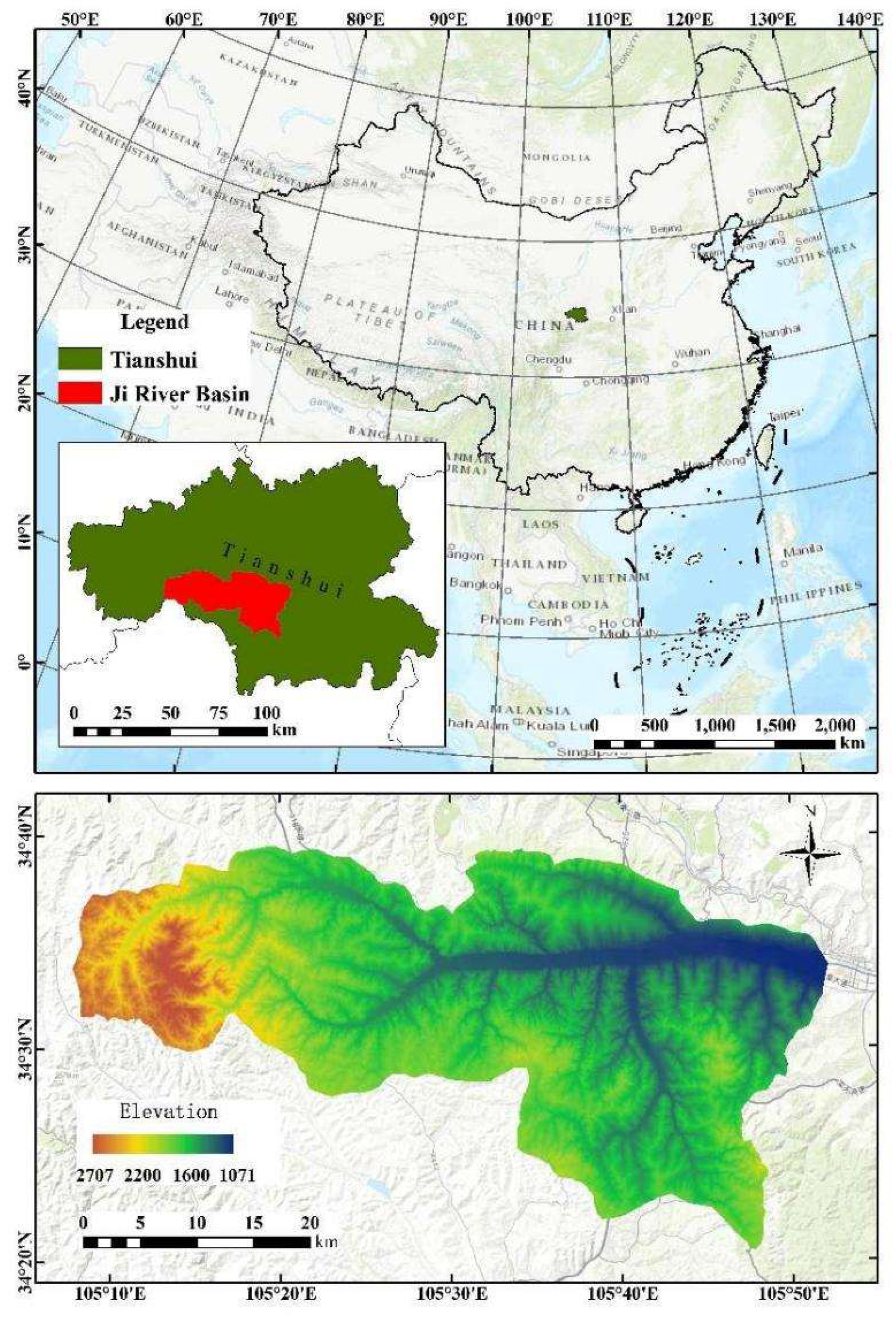
Figure 2.
Spatial distribution of different RSEI quality levels in the Ji River Basin in 1986, 1996, 2006, 2016, and 2024.
Figure 2.
Spatial distribution of different RSEI quality levels in the Ji River Basin in 1986, 1996, 2006, 2016, and 2024.
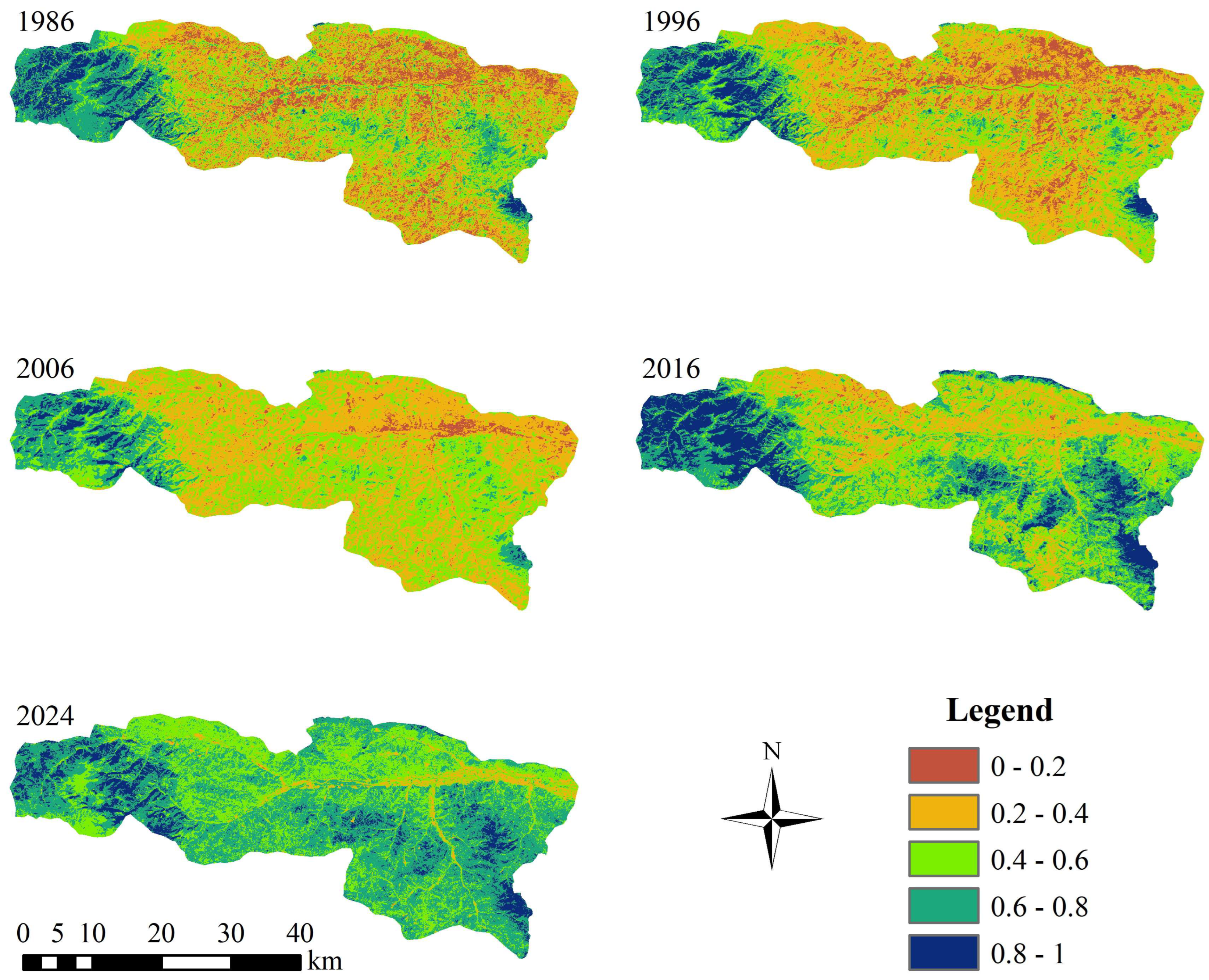
Figure 3.
Stacked column chart of different RSEI quality levels percent in the Ji River Basin from 1986 to 2024.
Figure 3.
Stacked column chart of different RSEI quality levels percent in the Ji River Basin from 1986 to 2024.
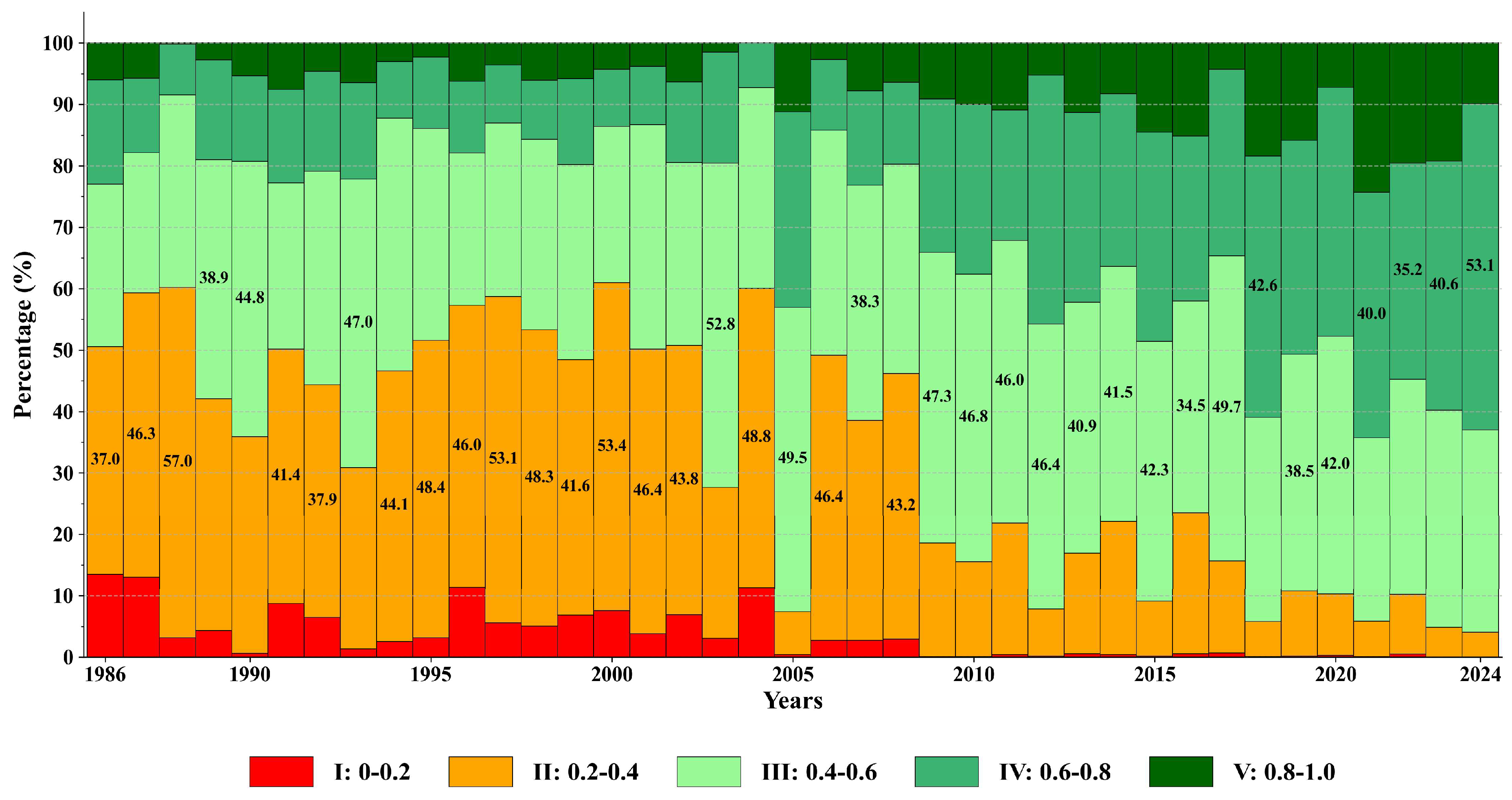
Figure 4.
RSEI change trend chart in different periods in the Ji River Basin from 1986 to 2024.
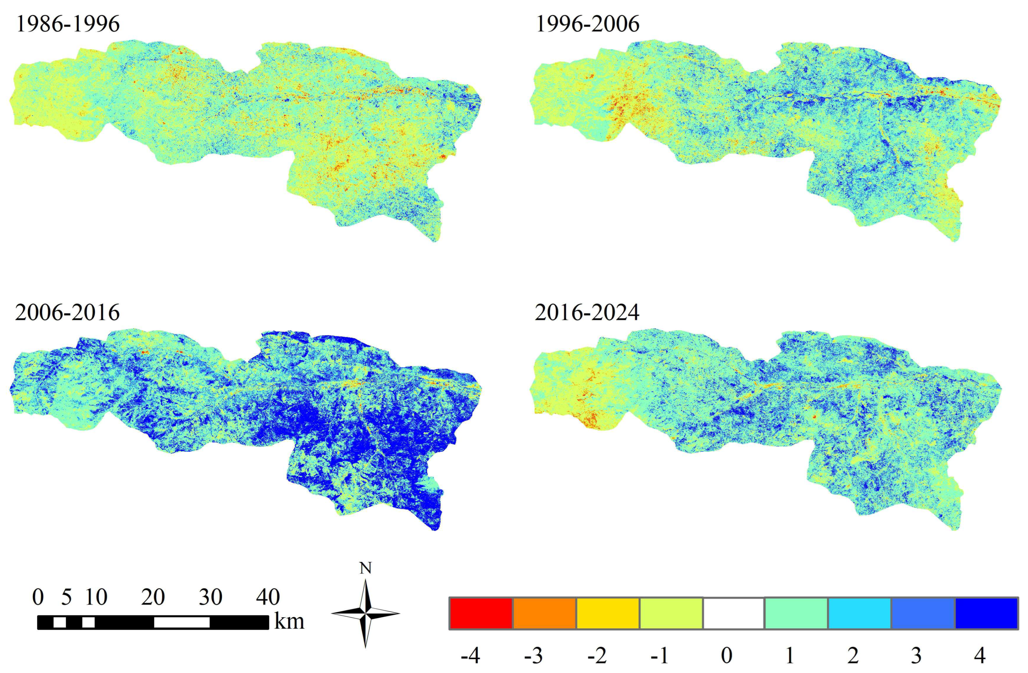
Figure 5.
Stacked column chart of RSEI trend change area percentages in different periods in the Ji River Basin from 1986 to 2024.
Figure 5.
Stacked column chart of RSEI trend change area percentages in different periods in the Ji River Basin from 1986 to 2024.
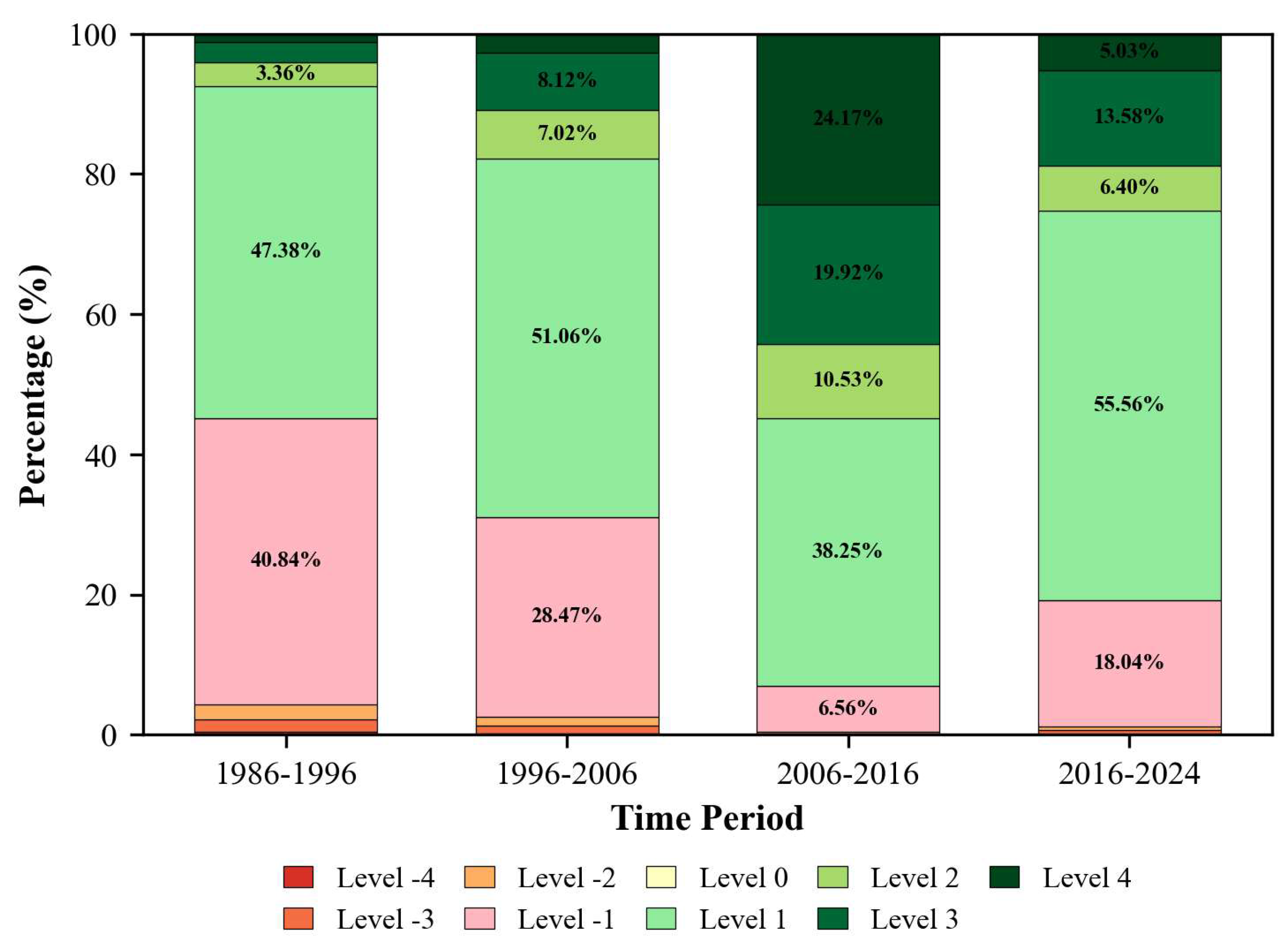
Figure 6.
LISA cluster maps (1986–2024) illustrating spatiotemporal patterns of RSEI autocorrelation. Color codes: pink (HH clusters), light blue (LL clusters), red (HL outliers), blue (LH outliers), gray (non-significant).
Figure 6.
LISA cluster maps (1986–2024) illustrating spatiotemporal patterns of RSEI autocorrelation. Color codes: pink (HH clusters), light blue (LL clusters), red (HL outliers), blue (LH outliers), gray (non-significant).
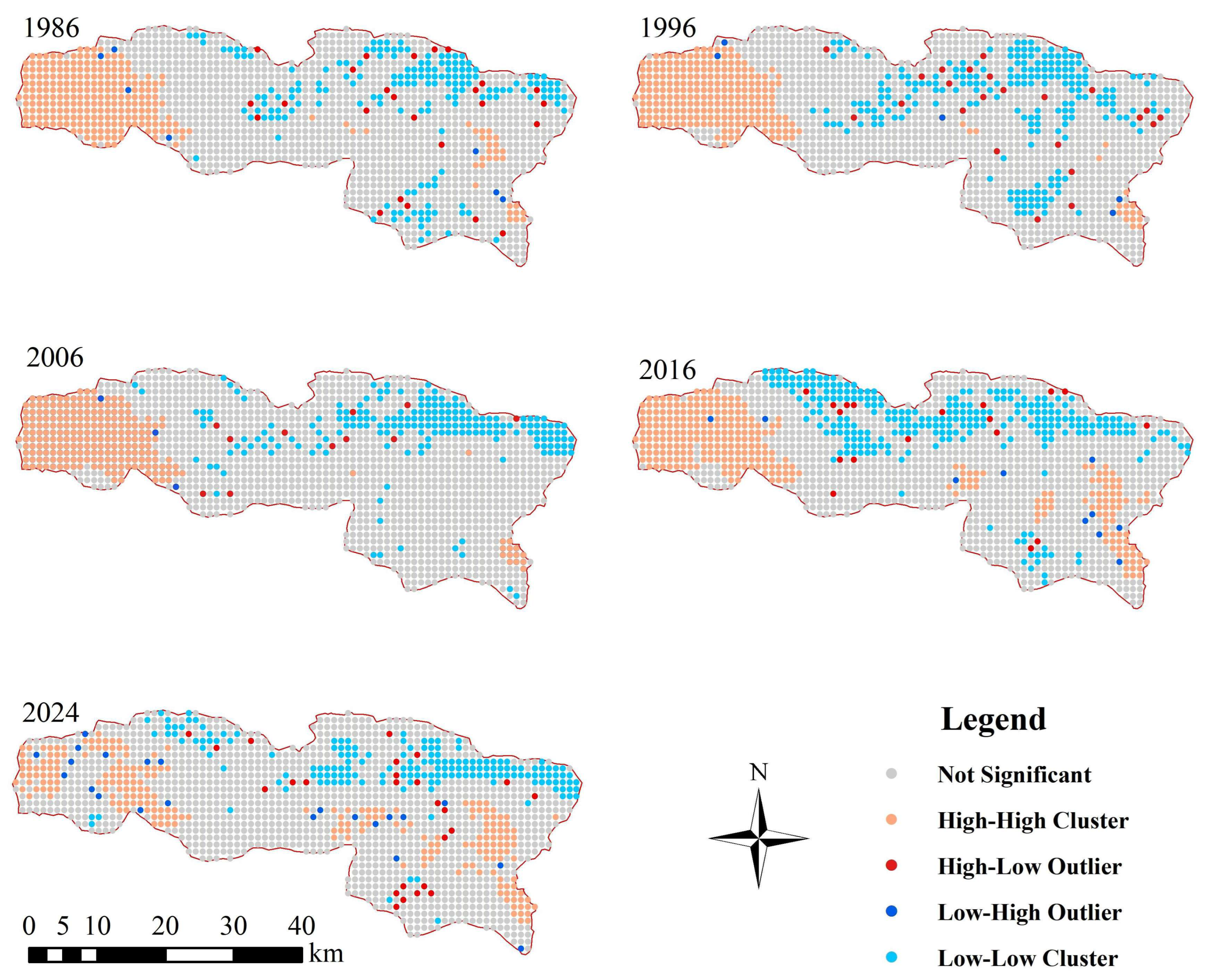
Figure 7.
Heatmaps of RSEI Values Across Topographic Factors in the Ji River Basin. (a) Spatiotemporal distribution of RSEI by elevation gradients (1986–2024); (b) Spatiotemporal distribution of RSEI by slope gradients (1986–2024); (c) Spatiotemporal distribution of RSEI by slope aspect (1986–2024), with aspect categories: N, NE, E, SE, S, SW, W, NW, and -1 (horizontal flat areas); (d) Spatiotemporal distribution of RSEI by TPI (Topographic Position Index) (1986–2024).
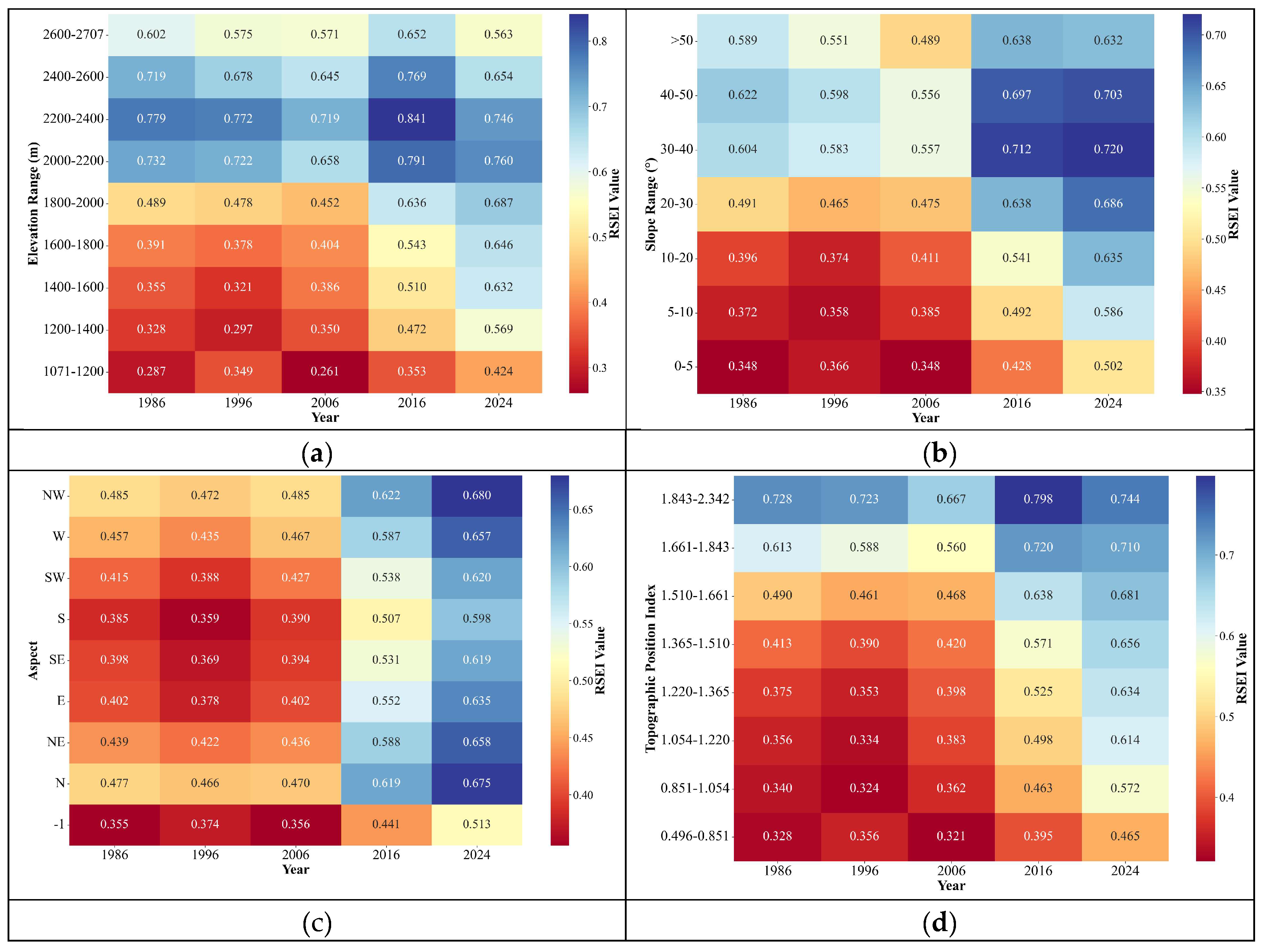
Figure 8.
Heatmap of RSEI Values Across Road Network Density Levels (0–8) and Years (1986–2024).
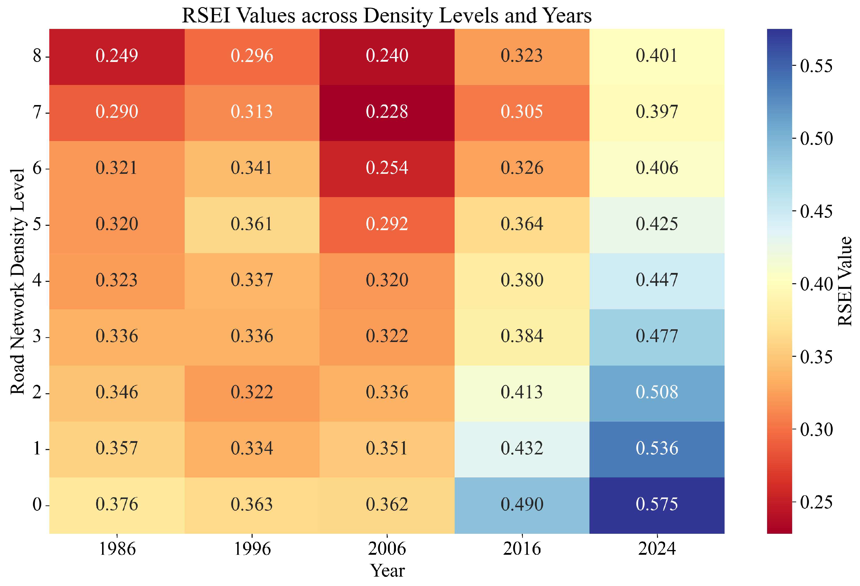
Figure 9.
Ecosystem Resilience Mapping of the Ji River Basin (2024).
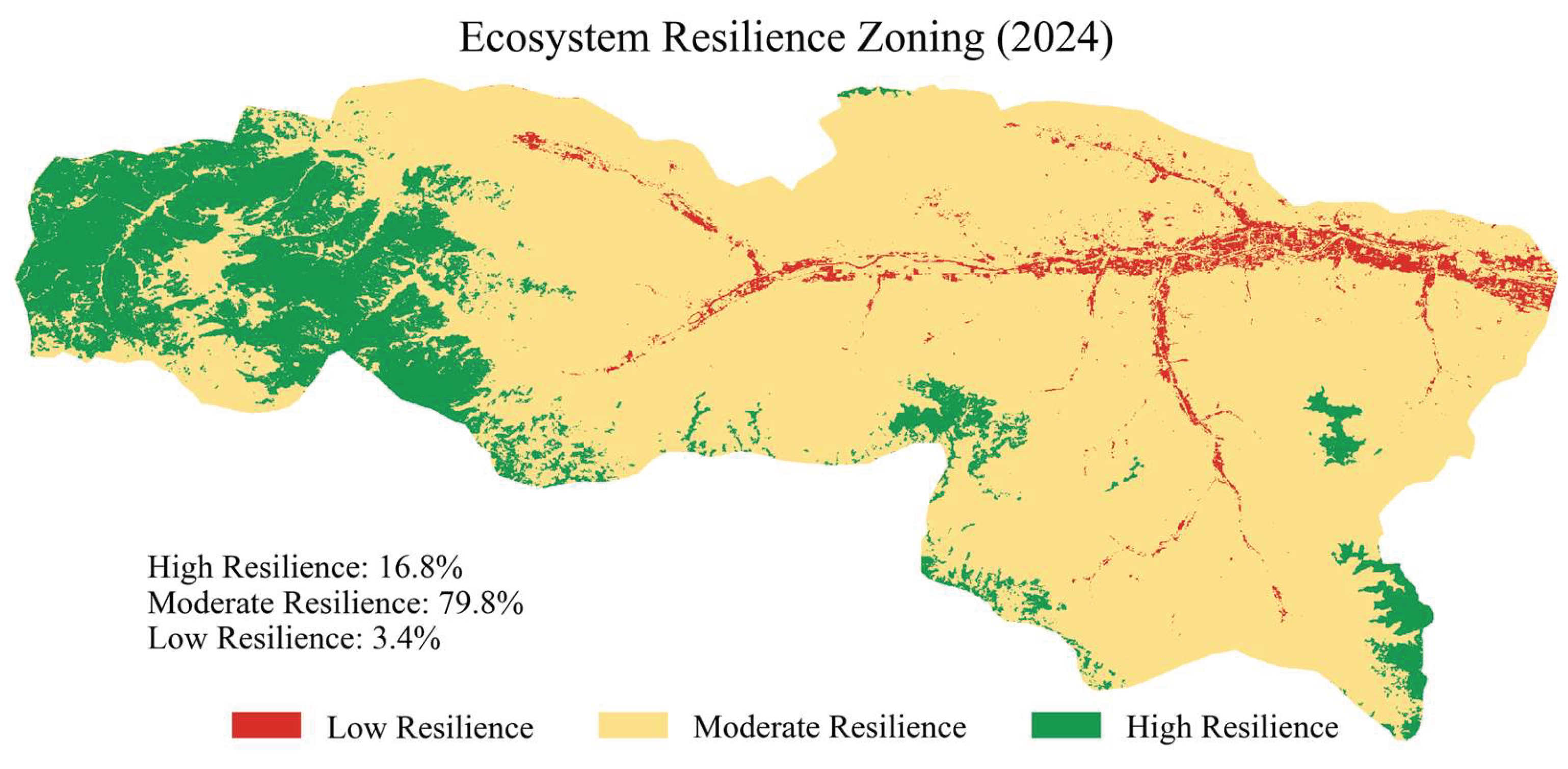

Table 1.
Introduction to research data.
| Sensor | Temporal Range | Dataset Path (GEE) | Band Mapping (SR/ST → Standardized) | Thermal Band |
|---|---|---|---|---|
| Landsat 5 TM | 1986–2011 | LANDSAT/LT05/C02/T1_L2 | [‘SR_B1’,’SR_B2’,’SR_B3’,’SR_B4’,’SR_B5’,’SR_B7’,’ST_B6’] → [‘Blue’,’Green’,’Red’,’NIR’,’SWIR1’,’SWIR2’,’TIR’] | ST_B6 |
| Landsat 7 ETM+ | 2012 | LANDSAT/LE07/C02/T1_L2 | ST_B6 | |
| Landsat 8 OLI | 2013–2024 | LANDSAT/LC08/C02/T1_L2 | [‘SR_B2’,’SR_B3’,’SR_B4’,’SR_B5’,’SR_B6’,’SR_B7’,’ST_B10’] → [‘Blue’,’Green’,’Red’,’NIR’,’SWIR1’,’SWIR2’,’TIR’] | ST_B10 |
Table 2.
PCA Results for Key Representative Years in the Ji River Basin.
| Year | PC Layer | Eigenvalue | Contribution (%) | Cumulative (%) |
|---|---|---|---|---|
| 1986 | PC1 | 0.078 | 89.47 | 89.47 |
| 1986 | PC2 | 0.006 | 6.66 | 96.13 |
| 1996 | PC1 | 0.091 | 90.09 | 90.09 |
| 1996 | PC2 | 0.006 | 5.73 | 95.82 |
| 2006 | PC1 | 0.035 | 84.76 | 84.76 |
| 2006 | PC2 | 0.005 | 11.20 | 95.96 |
| 2016 | PC1 | 0.061 | 89.29 | 89.29 |
| 2016 | PC2 | 0.006 | 9.01 | 98.30 |
| 2024 | PC1 | 0.029 | 82.78 | 82.78 |
| 2024 | PC2 | 0.004 | 12.74 | 95.52 |
Note: PCA was performed on the covariance matrix of Min-Max normalized indicators ([0,1] scale). Eigenvalues represent absolute variance on the normalized scale. PC1 contribution rates consistently exceed 82%, meeting the RSEI framework requirement (Xu, 2013) that PC1 should explain >70% of total variance. Cumulative contributions of PC1+PC2 >95% across all years ensure minimal information loss during dimensionality reduction.
Table 3.
RSEI grading evaluation table.
| RSEI Range | 0-0.2 | 0.2-0.4 | 0.4-0.6 | 0.6-0.8 | 0.8-1 |
|---|---|---|---|---|---|
| Level | I | II | III | IV | V |
| Description | Bad | Poor | Moderate | Good | Excellent |
Table 4.
Decision rules for ecosystem resilience classification.
| Resilience Zone | LISA Cluster | Elevation (m) | RSEI (2016–2024 mean) | Basin Area (%) |
|---|---|---|---|---|
| High-Resilience | HH (p<0.05) | >1,800 | >0.6 | 16.84 |
| Low-Resilience | LL (p<0.05) | <1,500 | <0.4 | 3.37 |
| Moderate-Resilience | Non-significant or outliers (HL/LH) | 1,500–1,800 or outside high/low criteria | 0.4–0.6 or mixed | 79.80 |
Note: All criteria must be met simultaneously for High/Low zones; the Moderate zone includes all non-qualifying areas.
Table 5.
Global Moran’s I index and z-scores for spatial autocorrelation analysis (1986–2024).
| Year | Moran’s I | z-score |
|---|---|---|
| 1986 | 0.614 | 33.30 |
| 1996 | 0.684 | 36.68 |
| 2006 | 0.691 | 37.49 |
| 2016 | 0.666 | 36.15 |
| 2024 | 0.445 | 24.18 |
Note: All values are significant at p < 0.01 (999 permutations).
Disclaimer/Publisher’s Note: The statements, opinions and data contained in all publications are solely those of the individual author(s) and contributor(s) and not of MDPI and/or the editor(s). MDPI and/or the editor(s) disclaim responsibility for any injury to people or property resulting from any ideas, methods, instructions or products referred to in the content. |
© 2026 by the authors. Licensee MDPI, Basel, Switzerland. This article is an open access article distributed under the terms and conditions of the Creative Commons Attribution (CC BY) license (http://creativecommons.org/licenses/by/4.0/).
Copyright: This open access article is published under a Creative Commons CC BY 4.0 license, which permit the free download, distribution, and reuse, provided that the author and preprint are cited in any reuse.


