
Submitted:
26 January 2026
Posted:
27 January 2026
You are already at the latest version
Abstract
We propose a mechanism for generation of vorticity in a rotating cylindrical shear flow and predict the effect of background rotation through three-dimensional linear stability analysis and direct numerical simulations (DNSs). Our linear theory predicts a positive feedback of angular momentum for moderate rotation rates that agree well with early time evolution of DNSs with weak rotation. These runs show the growth of low azimuthal wavenumber modes of instability at early times with subsequent onset of centrifugal instabilities that arrests the initial spin-up of the core. For stronger background rotation, we observe the emergence of helical modes of instability from very early times which drain angular momentum out of the vortex core. We discuss a possible caveat of the DNS results with regards to the choice of our domain size that appears to influence our prediction for low Rossby numbers and its implications for understanding the emergence and growth of large-scale vortices as commonly observed in DNSs of turbulent convection as well as natural flows in astrophysical and geophysical contexts.
Keywords:
rotating flows
; cylindrical shear flow
; vortex stability
; angular momentum transport
; centrifugal instability
; direct numerical simulation
1. Introduction
Direct numerical simulations of a variety of rotating turbulent systems, such as convection (Guervilly et al. 1, Julien et al. 2), stratified turbulence (Marino et al. 3, Oks et al. 4) and double-diffusive convection (Moll and Garaud 5, Sengupta and Garaud 6) have reported the emergence of large scale vortices (LSVs) that is indicative of a basic underlying instability that works towards sustaining these coherent structures in rotating environments. In an attempt to possibly identify this inherent mechanism that drives LSVs in rotating turbulence, we present a simplified analytical model of a vertical shear flow in a uniformly rotating system and study the growth of interfacial instabilities across the boundary of the flow. Through an asymptotic method, we investigate the linear stability of the flow and quantify the radial flux of axial angular momentum to predict regimes that could possibly spin up the core of the flow.
The stability of a column of fluid in a rotating environment has been a topic of many studies beginning with the early works of Hocking and Michael [7], Ponstein [8], Gillis [9], Alterman [10], Pedley [11] to later investigations using linear stability theory ([12,13,14]) as well as experiments reporting helical modes of instabilities in the context of rotating jets ([15]). Most of these works investigated the development of the capillary instabilities which are dominated by effects of surface tension balancing the outward centrifugal force leading to the saturation of the growing instability. The effect of viscosity has also been investigated on the growth and saturation of these instabilities by Hocking [16], Kubitschek and Weidman [17], Coppola and Semeraro [18]. The effect of a uniform circulation surrounding a cylindrical vortex sheet has been explored by Rotunno [19] with linear theory predictions for growth of unstable modes. In this work, we explore the effect of a uniform background rotation on the stability of a analogous flow as a simplified model for studying the growth of large scale vortices (LSVs) reported in recent numerical studies and also observed on various scales in nature. Recent efforts to explain the formation of such patterns in the oceanic context have concluded of its dependence to relevant parameters ([20]) albeit with semi-analytic or two-dimensional numerical simulations. This work attempts to simultaneously present DNSs of a idealized model for a vortex in form of a shear flow in a uniformly rotating triply-periodic domain.
In Section 2, we present a linear stability analysis of our toy model setup in a perturbative approach to deal with the full rotating problem in order to estimate the effect of the instability on the angular momentum budget of the shear flow. Section 3 presents numerical calculations incorporating effects of viscosity (for moderate values of Reynolds numbers) to test the predictions of our linear theory and also predicts the final non-linear outcome of this simplified picture of our vortex model. We conclude in Section 4 by discussing our findings and its implications for generation of LSVs in rotating environments and suggest improvements possible to make our proposed model approach more realistic conditions encountered for these environments
2. Linear Stability of a Rotating Cylindrical Shear Flow
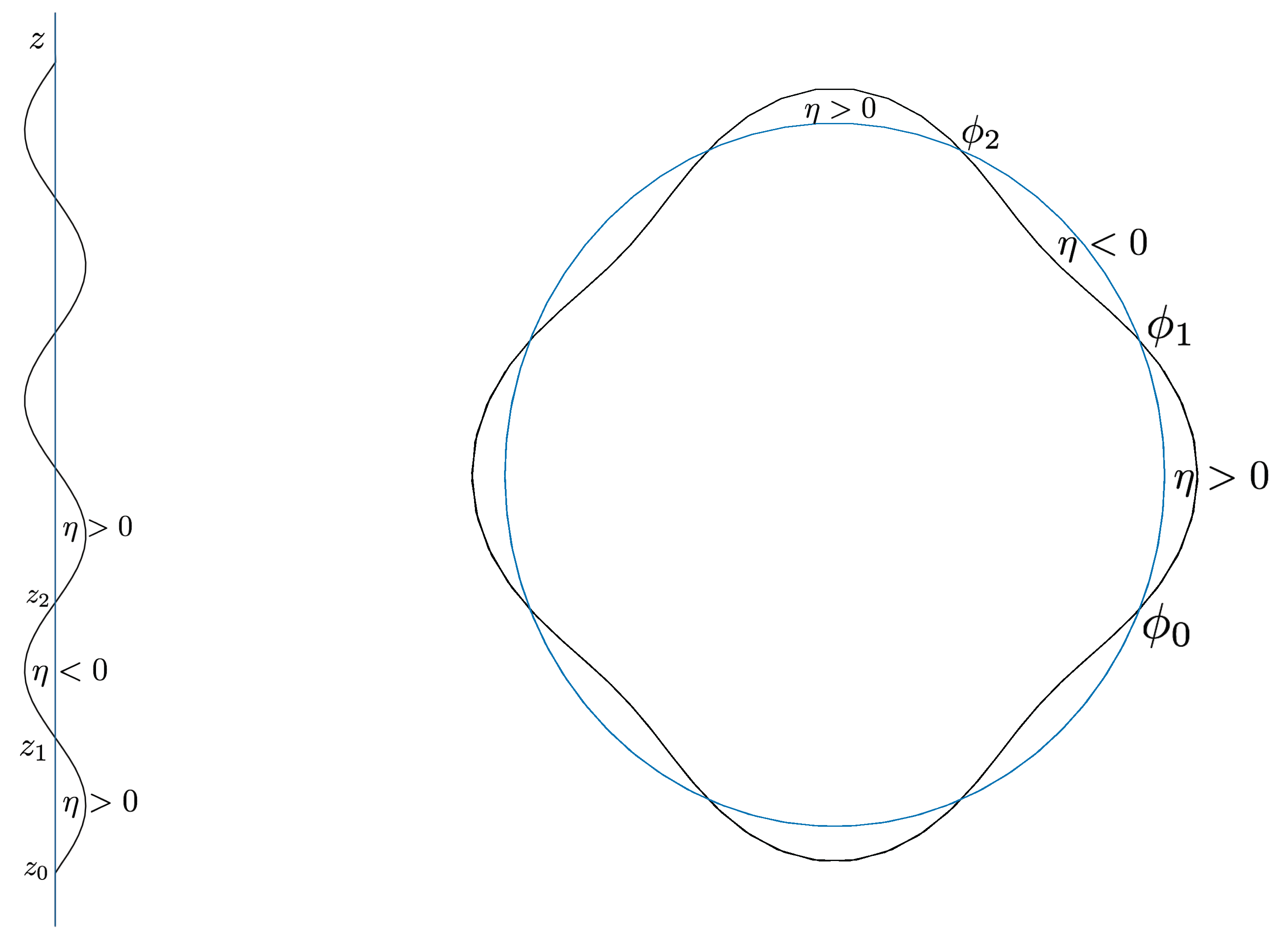
We begin by investigating the linear stability of a simple cylindrical shear flow in a rotating incompressible fluid, ignoring effects of viscosity and stratification. We consider a fluid rotating at an angular velocity , whose direction defines the vertical (z-axis). Within that fluid, we consider a cylindrical region of radius R, aligned in the z-direction, centered at . Within this cylinder, the fluid is assumed to rotate with an angular velocity, (with respect to the background), and flow along the z- direction uniformly with velocity . Outside the cylinder, the fluid has vertical velocity , and is rotating at a rate with respect to the background (see Figure 1). We calculate the unstable eigenmodes associated with this flow field and study their role in the evolution of the net angular momentum of the fluid in the cylinder. For simplicity, we assume the system is periodic in z, and study it in the interval only.
2.1. Governing Equations
For the model described above, the background velocity of the fluid (on top of the global rotation) is given by
where is the cylindrical radius. To ensure that this flow is in a steady state, the background pressure must satisfy
with the + and − signs corresponding to the regions inside and outside , respectively. As a result, note that the radial pressure gradient is discontinuous at when , but can be made continuous by suitable matching i.e.
We now consider perturbations and p to the flow and pressure respectively satisfying and . Linearizing the full equations around the background state and assuming incompressibility for the flow, the perturbation equations are given by
where, in cylindrical coordinates and as mentioned earlier, viscosity has been ignored. Using the following ansatz1 for each of the velocity components and for the pressure p
where and both m and n are both integers, we can reduce the set of perturbation equations within and outside the cylinder to
with
where, as before, the + and − signs correspond to inner () and outer () regions respectively. Taking the complex conjugate of the above equations, we can readily see that if a solution with growth rate satisfies these equations, then its complex conjugate also satisfies the same equations with growth rate . This implies that it suffices to describe the unstable modes in half of the parameter space. Hence, we restrict our study to but allow m to take both positive and negative values, as is commonly done in the literature in studies of temporal flow instability (e.g. [21]).
The first three equations can be combined to express the velocity fields in terms of the pressure perturbation as
Using these expressions in the incompressibility condition (7d) yields an equation for the pressure, namely
with
By imposing that the pressure has to be regular at and tends to zero for large r, we can write solutions in terms of the modified Bessel functions given by
where, without loss of generality, we selected the root of Eq 10 so that . Indeed, using the parity properties of the Bessel functions, it can be readily shown that solutions for cases with are obtained simply by reversing the sign of . Using these solutions, and the standard recursion relations for the derivatives of the Bessel functions given by
we define
The solutions for the velocity components can then be expressed as
The so far unknown amplitudes and are related to one another through the matching conditions at the interface between the inner and outer fluid. At any point in time, this interface is located at the position where is its radial displacement with respect to the rest position at .
The kinematic condition relates the function to the radial velocity of the fluid at any point along the interface, and implies
Linearizing this equation for small displacements, we get
which, using the ansatz (6) and a similar one for , namely
reduces to
where, for simplicity, we define
Note that without loss of generality, we can chose so that
where
As a result, using Eq 8, we see that
This expression, when combined with Eq 15, provides two equations that effectively relate to and , respectively.
A third equation between , and can be obtained from the only other allowable interfacial matching condition in an inviscid fluid, namely the matching of the pressure. Recall however that, for a differentially rotating fluid (i.e. ), the local centrifugal force induces a jump in the background pressure gradient at (see Eq 2) which has to be taken into account in the matching procedure. We therefore match the total pressure at the interface located at . After linearization, this implies the continuity of across the interface, which (using Eq 2 and the ansatz for p and ) becomes
The second term on both sides is the contribution from the centrifugal force, which cancels out unless .
Combining Eqs 15a and (24), we can now eliminate all unknown amplitudes , and to obtain the dispersion relation for the growth rate as
This equation must usually be solved numerically for growing modes () to reveal different regimes of instability in the flow. However, in some limiting cases, analytical or semi-analytical solutions exits which are discussed next.
2.2. Limiting Cases:
2.2.1. Non-Rotating Case () :
Without any background or differential rotation of the tube, we have ; so, the dispersion relation becomes
with the superscript denoting quantities associated with the non-rotating flow, i.e.
Eq (26) can now be solved analytically for , and the solution corresponding to the growing mode of instability is
With a little algebra, this result can be used to show that
which will be used in what follows. Eq (27) also illustrates the basic nature of the shear instability with the shortest wavelengths being the fastest growing ones as is typically obtained for the standard inviscid planar shear instability. The information about the geometry is solely contained in the quantities and . Note that in the limit of large m,k, ([22]), using which we further recover the growth rates for the plane parallel shear case with
2.2.2. Rigid Rotation ():
In this case, the centrifugal term of the right hand side of the dispersion relation given by (25) vanishes, and so it reduces to
This equation must usually be solved numerically, but can be solved asymptotically in the regime of weak rotation for which
Using the following ansatz for the growth rates in the above form of the dispersion relation
which implies
where is assumed to be . By linearizing Eq (26) in small , we can compute the correction to the growth rate due to rotation, as
Using the expression for the non-rotating growth rates given by Eq 27 in the limit of large k, it can further be shown that
We see that, when combined with the ansatz given by Eq (32), the first-order corrections to the non-rotating growth rates have opposite sign as m i.e. positive-m are stabilized by weak rotation whereas negative-m are further destabilized. Furthermore, this ansatz also reduces to the expression given by Eq 29 in the limit of vanishing . In other words, weak rotation only affects the growth rates to linear order in for large values of k.
2.2.3. Differential Rotation ():
For the differentially rotating case, the full dispersion relation (Eq (25)) needs to be solved numerically. It can, however, also be solved analytically when both rotation and differential rotation are weak. As before, we assume the ansatz given by Eq 32, with now assumed to be . This implies
To linear order in and , we also have ; so, linearizing the full dispersion relation (Eq 25) in the limit of small , we obtain
Using the expression for given by Eq (33), one can write the expression for the growth rates in the limit of large m and k as
the real part of which illustrates the contributions to the growth rate in terms of the vertical and azimuthal components of shear instabilities.
2.2.4. Axisymmetric Mode ():
When Eq (25) reduces to
with and , which must again usually be solved numerically. In the special case of pure rotation with no vertical background flow i.e. , for which and , we recover the dispersion relation for a jet in pure rotational motion inside a rotating medium, as derived by Alterman [10]:
which is identical with their Eq 66 (which follows from their Eq 62, but for an error in the sign of the first term on the right hand side) when both the fluids inside and outside the cylinder have uniform density (of 1) and there are no capillary effects.
2.2.5. Asymptotic Limit of Large k:
In the limit , as well, and we can use series expansion for the modified Bessel functions ([23]) to write
independently of m, as long as . Neglecting the terms of for large values of k, and noting , the full dispersion relation then reduces to
This can be solved analytically for the growing mode of instability as
and recovers Eq 38 in the limit of weak rotation. The real part of this general expression clearly shows the contribution from the shear (both vertical and azimuthal) and centrifugal terms. The centrifugal term is always destabilizing for an angular momentum profile that decreases outwards (i.e. which is the condition for the occurrence of the well-known centrifugal instability. The shear term is also destabilizing but its contribution is determined by the relative signs of .
2.3. Numerical Solutions of the Dispersion Relation
In this section, we present few representative numerical solutions of the dispersion relation for given set of values of , (25) using the numerical root-finding method described by Barrodale and Wilson [24] (see [25] for a discussion on the limitations of this method) combined with the Bessel function approximation routines provided by Zhang and Jin [23]. To do so, we first non-dimensionalise our system with respect to the radius R and the vertical shear ) and hence define the non-dimensional quantities as
We select only the roots of (25) for the growth rate that have positive real part, and when more than one exist, we report only the largest one as a function of the background rotation rate to illustrate the effects of rotation and differential rotation in determining the fastest growing modes.
2.3.1. Comparison with Analytical Results Without Rotation
We first test the results of our solver in absence of rotation () and compare the numerical values of maximum growth rates with the analytical expression given by Eq (27). Figure 2 illustrates the exact agreement obtained between the two as a function of the vertical wavenumber for two choices of the azimuthal wavenumber . For higher values of m, both the numerical and analytic solutions become indistinguishable from the solutions for with increasing values of m, but the agreement between the two remains exact. Also, the solutions for the mode is identical to that for the mode due to the symmetry properties of the modified Bessel functions, which is why they are not shown. As expected from pure inviscid shear instabilities, the growth rate of the modes increase with increasing wavenumbers (i.e. increasing and ).
2.3.2. Comparison with Large Asymptotic Formula for Differentially Rotating Case
We next test our numerical solutions in the limit of large against the asymptotic approximation (Eq 43) for a differentially rotating case. Figure 3 illustrates the agreement between the numerical and asymptotic predictions for and 2 with increasing values of for an example case in which we have selected . As is readily seen, for large enough values of , the numerical and asymptotic results agree well with each other, illustrating that the numerical solver works well in this limiting case as well. The effect of rotation and differential rotation on the growth rate of the modes is discussed in Section 2.4.
2.3.3. Obtaining Solutions for High Rotation Rates or at Low Values of k
In general, finding numerical solutions of the full dispersion relation given by Eq 25 using the root-finding method employed here (which is based on a Muller algorithm) requires the user to supply a sufficiently accurate guess to initialize the iterative solver. To do this, we use one of two possible alternatives (depending on which one is more successful). In some cases we fix m and to the desired values, and use the exact non-rotating expression given by Eq 27 as a starting guess and gradually increase the rotation rate and differential rotation towards the target parameter values, each time using the numerical solution obtained for one set of parameter as a guess for the next set of parameters. Alternatively, we can also fix the value of m and of the rotation rates and use the asymptotic approximation given by Eq 43 for a sufficiently high value of as a starting guess instead, and gradually decrease to obtain numerical results at the desired wavenumber. With this continuation technique, we have been able to find solutions of Eq 25 for almost all sets of parameters. We discuss these results in the following section illustrating the nature of the associated (centrifugal and shear) instabilities.
2.4. Effect of Rotation
In this section, we present results on the linear stability of the rotating sheared tube model described in Section 2.1 and clarify the effects of shear, rotation and differential rotation.
2.4.1. Shear with Uniform Rotation
We begin by considering the uniformly rotating case i.e. when . Figure 4 shows the growth rate, for two different vertical wavenumbers and 5, for , as a function of the rotation rate . We also compare the asymptotic predictions for the growth rates for low rotation rates (as given by Eq (32)) with our numerical solutions which shows agreement with the numerical values for . It clearly shows that the negative m- modes are destabilized while the positive m-modes are stabilized by rotation. This trend, which is predicted by the low asymptotic theory, persists and intensifies at higher rotation rate. We therefore predict that for rapidly rotating systems, negative m-modes could prevail, while for slowly rotating systems, both negative and positive m-modes could be present during the linear growth phase of the instability. We also see, as expected, that higher k modes are more unstable, at least in this inviscid limit.
2.4.2. Shear with Background Rotation and Differential Rotation
We now present illustrative results showing how the growth rate of the , modes vary with both rotation and differential rotation . For simplicity, we assume , so positive values of correspond to centrifugally destabilized systems, while negative values of correspond to centrifugally stabilized systems. As in Figure 4, we also compare these numerical results with the asymptotic predictions for weak rotation (see Eqs. 32-34). Figure 5 demonstrates that the numerical results agree well with the asymptotic predictions for growth rates for with different choices of . We also see that the difference between the behavior of the and modes with increasing (at a fixed value of ), that makes the modes more unstable but stabilizes the mode. This effect can be understood from the asymptotic expression for the growth rates at large (given by Eq 43) with the contribution from the centrifugal instabilities given by the term ), being of different signs depending on the sign of m.
2.5. Transport of Angular Momentum
Having studied the stability of the system to small perturbations, we now investigate how these perturbations influence the rotation of the cylinder itself. In this section, we go back to dimensional quantities. The specific angular momentum expressed in cylindrical coordinates is given by
where
In a non-dissipative system, the conservation of angular momentum requires
which, upon integration over the volume of the cylinder between 0 and , gives the net rate of change of angular momentum within as
where denotes the volume of the cylinder contained in , is the unit vector directed normally outward on the surface element , so and, given the periodicity in z, (i.e. only the integral over the surface matters).
Using Eq (48), at , we then have
where the first integral vanishes due to mass conservation (Eq (5)). The remaining integral over and z needs to be taken with care since the quantities and are evaluated differently depending on the sign of the displacement . The calculation is presented in Appendix B, and provides the net expression for the angular momentum flux into the tube:
where we have defined
and indicates that the quantity is evaluated at . Using the solutions and given by (15), we can write
where we have defined
Using the solutions for the pressure given by Eq 12, and the kinematic boundary condition expressed by Eq (19), we can finally express the rate of change of angular momentum in the cylinder explicitly as a function of and other properties of the unstable modes (see Appendix B for detail), as
where the functions and are given by
with and . Using this expression, we can obtain the angular momentum change of the tube for the limiting cases considered already:
- 1.
- Non-rotating case () : In the non-rotating limit, and thus,since are real according to Eq 14. Hence, it is readily seen that there is no net change of angular momentum of the tube in absence of rotation, as expected.
- 2.
-
Rigid rotation () : for this scenario,If we further assume that is small and since , thenHence, the rate of change of angular momentum can further be simplified towhich can be shown to be positive (see Figure ) for growing modes (), implying that there is a net flux of angular momentum into the tube. Note that this expression can also be recovered independently by working with the low asymptotic expressions for and (see Appendix A).
- 3.
- Axisymmetric mode (): In this case, and , hencewhich could be either positive or negative depending on the signs and relative values of and . However, the only way to have is to have the outer cylinder counter-rotating (i.e. is sufficiently negative).
- 4.
- Asymptotic limit of large k: in this limit, , which implieswhich can only be negative if m itself is larger than k or if is sufficiently negative.
To find the direction of angular momentum transport in general (i.e. not in one of these above limits), we directly compute the expression given by Eq 56 using the numerical solutions for the fastest growing modes obtained in Section 2.3. Figure 6 shows illustrative results obtained for and modes for a range of values of the rotation rate and for a range of values of . Red regions in the figure imply net influx of angular momentum into the cylinder and blue regions imply net outflux of angular momentum from of the cylinder. For the case, the numerical results show a distinct region in the parameter space with positive flux of angular momentum into the cylinder which becomes negative for sufficiently large rotation rate or sufficiently large differential rotation. This predicts a spin-up mechanism for the shear flow for low to moderate rotation rates if is the dominant mode of instability in the flow. For , we predict a similar spin-up through the linear instability across almost the entire parameter space in , except in the case of very weak rotation for a narrow range of values of or much greater than . For modes with , the numerical solution always predicts an inward flux of angular momentum into the cylinder for all values of , which are hence not plotted in Figure 6. This is also consistent with the asymptotic expression for large k (give by Eq 63) for . In the following section, we test these predictions for the spin-up mechanism of our idealized shear flow setup through direct numerical simulations.
3. Numerical Simulations
In order to test our findings regarding the nonlinear evolution of the rotating cylindrical shear flow, we now run some direct numerical simulations (DNSs) of a model that is similar (though not exactly identical) to the one described in Section 2. For this purpose, we use the pseudo-spectral triply periodic PADDI code (Stellmach et al. [26], Traxler et al. [27]) that has been modified to include rotation (Moll and Garaud [5], Sengupta and Garaud [6]) as well as the imposed forcing term. In all that follows, we non-dimensionalize the flow velocity with and the distances with the radius of the cylinder so that . With this setup, we define the background flow to be the following top-hat form for the z-component of velocity:
with (though we also present a test case with ) and being the distance from the center of the tube. The computational domain is of dimensions .
3.1. Non-Dimensional Governing Equation
The non-dimensional Navier-Stokes equations for our problem setup are given by
Note that for the DNSs, the effect of viscosity must be retained to ensure stability. We see the usual non-dimensional parameters appear, such as the Reynolds number (where is the viscosity) and the Rossby number, . A forcing term is imposed on the system, which drives the desired cylindrical shear flow (given by Eq 64) provided is defined as:
To test the predictions of our model, we investigate the sign of the angular momentum transport during the early development of the instability by computing the flux of angular momentum through the cylinder of radius r centered at , at each time t, as:
To do so, we first calculate from the Cartesian components of the velocity vector returned by PADDI using the following transformations:
and, where at each position ,
Using the azimuthal velocity , we also compute the average angular velocity as a function of the radial distance from the center of the domain at a given time t:
3.2. Typical DNS
We first present results for a single DNS at , and fairly large Reynolds numbers, to ensure that the results are not dominated by viscous effects (which were ignored in the analytical computations presented in Section 2).
For our DNSs at (that corresponds to a ), Figure 7 shows isocontours of vertical components of velocities for two runs A2 and A3 (as in Table 1) during the linear growth phase (left panels). Both these runs clearly show the emergence of a preferred mode with low values of the azimuthal wavenumber () and fairly high vertical wavenumber (), irrespective of the domain aspect ratio (the run A1 with the same aspect ratio as A3 also emerged with a similar mode). We now look at the results of our simulations more quantitatively.
3.2.1. Early Phase:
We compare the evolution of the run A3 with the predictions from our linear theory presented in Section 2, with regards to the direction of angular momentum transport. The left panel shows the profiles of the total angular momentum flux as a function of r, at selected times during the growth of the linear instability, showing a clear negative spike at , which should result in a positive flux of angular momentum into the cylinder. The right panel of Figure 8 shows the evolution of during the exponential growth phase of the linear instability, clearly demonstrating that the angular velocity within the region grows with time, and thus validates the feedback mechanism of angular momentum predicted from our linear theory (given by Eq 56).
We also calculate the average rate of rotation for the cylinder as
Figure 9 follows the evolution of (calculated according to Eq 71) for our DNSs A1 and A3. All these simulations illustrate the initial positive flux of angular momentum into the tube that significantly spins up the region inside .
3.2.2. Growth of Centrifugal Instabilities
Figure 8 shows that becomes positive near around , which halts the growth of the angular velocity for . To understand why this happens, we plot the vertically and azimuthally-averaged angular momentum profile, defined by
Figure 10 shows a radial decrease in the angular momentum profiles around , starting at the earliest time snapshot presented (). When is decreasing with increasing r, this angular momentum distribution is well-known to be unstable according to the generalized Rayleigh criteria for centrifugal instabilities ([28]) which requires
for any flow to be stable to perturbations. Any centrifugal instability is known to work against its causing mechanism and thus would act to stabilize this negative angular momentum gradient. However, from Figure 9, we see that the tube still continues to spin up (manifested in an increase of ) until the associated instabilities reach finite amplitudes (at ) for them to arrest further spin-up of the tube. The competing effects of an unstable angular momentum gradient and associated instabilities control the ultimate outcome of the nonlinear evolution of the spin of the tube, as narrated in the following section.
3.2.3. Nonlinear Evolution: Emergence of Negative Helical Structure
We followed the evolution of one of our low (A1) and high (A3) Reynolds number runs until a quasi-steady state was achieved to check for the final nonlinear outcome for the direction of rotation of the cylinder. At late times, as shown in the Figure 11 for the run A3, the flow through the cylinder (inside ) does not remain perfectly coherent anymore but gradually evolves into a weakly helical structure.
12 shows the time-evolution of the average rotation rate of the tube, (as defined by Eq 71) for both runs. Beyond the early phase of positive growth, the onset of centrifugal instabilities over time appears to make the tube marginally counter-rotating. In order to determine whether the negative rotation rate is intrinsic to the tube, or may be contaminated by the presence of its helical twist, we also propose an alternative way of measuring the average angular velocity of the tube by re-defining the center of the tube at a particular height z as
where is the Heaviside function. We over-plot the results (shown as symbols) in Figure 12 , which demonstrates the helical shape of the flow only influences our results beyond the initial phase of linear growth, when the center (as defined by Eq 74) does not shift much from the center of our domain. In the nonlinear regime, our alternative method gives a more continuous pattern in the evolution of the averaged rotation rate with time although the general conclusion with regards a weakly counter-rotating (i.e. with marginally negative ) flow seems to hold till the tube reaches a quasi-steady state.
3.3. DNSs at lower values
While our DNSs A1-A3 affirm the prediction from our model (described in Section ) for positive feedback of angular momentum into the tube at early times, our preliminary runs (B1-B3, C1-C2) for lower values of did not show any signs of spin up of the core of the tube (for ) even for the initial few snaps shots. This is demonstrated in Figure 13 for two set of runs (B1 and B2) which both show a decrease in the averaged rotation rate (as defined in Eq 71) early on in the simulations.
We also checked for the radial profiles of the Reynolds stress function (given by Eq 67) and the average angular velocity (given by Eq 70) at early times for one of these runs (B2) as shown in Figure 14,
which indeed demonstrates a negative flux of angular momentum from the region at all times. These runs still emerged with similar modes (low m, fairly high k) as the higher cases, but clearly do not conform to the expectation from the linear theory that predicts positive angular momentum feedback into the tube for such linearly unstable modes. In following section, we discuss a plausible cause of this discrepancy, to with our periodic domains that seems to problematic at low values when the results seem to be dependent on the horizontal extent of the domain.
4. Discussions
We have studied an idealized setup of an inviscid vertical shear flow through a cylindrical tube using linear stability analysis and predicted a positive feedback mechanism transporting angular momentum into the tube. Direct numerical simulations for an analogous setup at support our theoretical predictions for the positive feedback of angular momentum at early times, before the onset of centrifugal instabilities that arrest the growth of the spin-up of the tube. However, our preliminary DNSs with moderate () to strong () rotation seemingly do not agree with our model predictions. In context of studies of vortex dynamics, it has been pointed out in the literature by Pradeep and Hussain [29] that the use of triply periodic domains can often give incorrect results due to artificial zero circulation constraint inherent in periodic simulations. Following the recent work of Sutyrin and Radko [30], we performed additional runs (B3, B4 in Table 1) with half the vertical extent (for both B3 and B4) but double the horizontal extent (B4).
The corresponding time evolution of the average rotation rate of these two runs are compared in Figure 15 which clearly shows that the wider domain run spins up during early times (consistent with our linear theory predictions) unlike the other ones (B1-B3), all of whom showed no such signs of positive feedback of angular momentum with narrower horizontal extent of domains. These computations are substantially more expensive due to the larger resolutions ( in the horizontal direction for the B4,B5,C2 runs) needed to resolve the shear layers at the edge of the tube that occupies only a very small region at the center of the domain. However, from these numerical experiments, it is apparent that particular caution needs to be exercised in the choice of the domain size (compared to the radial extent of the tube) in order to ensure the DNS predictions are not influenced by the periodicity assumptions. The increasing computational cost for lower and/or higher simulations inhibits us from performing such robustness tests for our most rapidly rotating runs (C1, C2) at , but they would be important to establish the theory at very low values, particularly in context of the regime of emergence of LSVs as discovered in Sengupta and Garaud [6] for astrophysical flows.
Acknowledgement
This work received generous financial support from the Jack Baskin-Peggy Downes’ Baskin fellowship (2018-2019) and partial support from the National Science Foundation under Grant AST-1814327. The simulations presented were performed on the Hyades supercomputer, purchased using an NSF MRI grant, the Extreme Science and Engineering Discovery Environment (XSEDE) supercomputing facility Stampede 2, and the Cori supercomuter of the National Energy Research and Scientific Computing Center (NERSC), a DOE Office of Science User Facility, supported by the Office of Science of the U.S. Department of Energy (under Contract No. DE-AC02-05CH11231) at the Lawrence Berkeley National Laboratory through an Exploratory Allocation award titled "Performance of 3D pseudospectral code for astrophysical modeling on Cori KNL". The author would like to humbly thank Professor P. Garaud and Professor T. Radko for critical comments and suggestions throughout the course of this work, Dr. S. Stellmach for the use of the PADDI code and Dr. S. Dong for help in porting the code on the KNL nodes of Stempede 2 2. Figure 7 and 11 were rendered using VisIt, a product of the Lawrence Livermore National Laboratory.
Appendix A Appendix A
Appendix A.1. Asymptotic Approximations in the Limit of Weak Rotation
In this appendix, we present approximate solutions to the full rotating problem in the limit of small rotation rates (). We use the general ansatz for all perturbations given by
where the (0) superscript represent non-rotating values of the perturbation , and assume . Thus,
with , with .
For the non-rotating problem (i.e. for ), the velocity components (given by Eq 15) are given by
where and were defined in Eq 14. The pressure continuity condition at implies
Further, imposing the kinematic condition (given by Eq 16) gives us the dispersion relation (Eq 26) and the non-rotating values of growth rates (Eq 27) from which we obtain
Using the ansatz A1 in the set of governing equations (Eq 4b), we obtain the set of governing equation for the corrections to the perturbations in presence of rotation as
These equations can be combined to obtain a new equation for the pressure correction term as
The last term can be shown to vanish using the non-rotating solutions given above, so Eq A7 reduces to
which is the same equation as for the non-rotating pressure , and hence, without any loss of generality, we can therefore assume . By solving Eq A6a, we then find that the corrections to the velocity perturbations in presence of rotation are
Finally, using the kinematic condition at , we can obtain an expression for the correction term to the growth rate as
which recovers the earlier result (Eq 34) obtained directly from linearizing Eq 25 for weak rotation rates.
Appendix A.1.1. Angular Momentum Transport:
Using the analytical expressions derived above in the limit of small rotation rates, we can arrive at an approximate expression for the angular momentum transport. Using the following ansatz for and :
it can be shown that the rate of change of angular momentum into the cylinder, as derived in Section 2.5, is then given by
With some algebra, the required coefficients in the above ansatz are determined as
Hence, we can express the angular momentum flux expression as
where we denote the real part of the non-rotating growth rate as . This also recovers the rigidly-rotating expression given by Eq 61 for .
Appendix B
Appendix A.2. Derivation of Expression for Angular Momentum Transport
Axisymmetric case (m = 0)
For the axisymmetric mode, and at depend only on z and t, so
and hence, from Eq 51, we get
The difficulty in evaluating this integral becomes apparent when we recall that
where
and similarly for . So, the integral needs to be split into intervals of positive and negative values of , respectively (illustrated in the left panel of Figure B.1). Recalling the ansatz for given by Eq 21, we define to be three successive nodes of , such as, e.g.
Then, we let
where the integral containing vanishes. Likewise, we can evaluate
Finally, we find that the rate of change of the total angular momentum of the cylinder is
where we recall that from Eq 6, . Note that, in the last step, we have made use of the complex identity
From Eq Section 2.1, the axisymmetric solutions for and are given by
which further reduces the expression for angular momentum flux into the cylinder to
Thus, if , this expression is always positive implying positive influx of angular momentum into the cylinder. However, for sufficiently negative , could become negative resulting in the drainage of angular momentum out of the cylinder.
We can also rewrite the above expression in terms of by using Eqs 23 and A24, as
Figure B.1.
Illustration of the shape of the interface perturbed from (blue line) with an amplitude for axisymmetric (left) and non-axisymmetric (right) modes.
Figure B.1.
Illustration of the shape of the interface perturbed from (blue line) with an amplitude for axisymmetric (left) and non-axisymmetric (right) modes.
Appendix A.2.1. Non-Axisymmetric Case (m≠0):
Using a method similar to the one described above for the axisymmetric case, we can rewrite the integral of the Reynolds stress term over as
where , and are successive zeros () of (see Eq 21), as illustrated in the right panel of Figure B.1. For , they are for instance given by
while for , they are
For a given mode with wavenumbers , we can we can evaluate the integral given by Eq A28 in a manner very similar to and in the axisymmetric case above, to obtain
This finally yields
Now, combining Eq (15) and (19), we can write
with given by Eq 55. Inserting these expressions for the pressures in Eq (15), with some algebra, the net flux of angular momentum for the cylinder can be expressed in the form
where the functions and are given by
with and .
Appendix C
Appendix A.3. Derivation of Mass Conservation
To show that mass is exactly conserved in the formulation of the model setup described in Section (2.1), we compute the net flux of the flow across the cylinder by evaluating the integral
which has to be done separately for axisymmetric and non-axisymmetric cases, in a similar manner as Appendix B.
Axisymmetric case (m = 0)
by using the identity given by Eq (23), where .
Appendix Non-axisymmetric case (m≠0):
As in Appendix B, we can rewrite the integral over in Eq (A36) as
due to Eq (23), thereby implying
Thus, both for axisymmetric and non-axisymmetric modes, the net mass flux across the cylinder vanishes identically, guaranteeing mass conservation.
References
- Guervilly, C.; Hughes, D.W.; Jones, C.A. Large-scale vortices in rapidly rotating Rayleigh-Bénard convection. Journal of Fluid Mechanics 2014, arXiv:physics.flu758, 407–435. [Google Scholar] [CrossRef]
- Julien, K.; Knobloch, E.; Plumley, M. Impact of domain anisotropy on the inverse cascade in geostrophic turbulent convection. Journal of Fluid Mechanics 2018, arXiv:physics.flu837, R4. [Google Scholar] [CrossRef]
- Marino, R.; Mininni, P.D.; Rosenberg, D.; Pouquet, A. Inverse cascades in rotating stratified turbulence: Fast growth of large scales. EPL (Europhysics Letters) 2013, 102, 44006. [Google Scholar] [CrossRef]
- Oks, D.; Mininni, P.D.; Marino, R.; Pouquet, A. Inverse cascades and resonant triads in rotating and stratified turbulence. Physics of Fluids 2017, arXiv:physics.flu29, 111109. [Google Scholar] [CrossRef]
- Moll, R.; Garaud, P. The Effect of Rotation on Oscillatory Double-diffusive Convection (Semiconvection). The Astrophysical Journal 2017, arXiv:astro834, 44. [Google Scholar] [CrossRef]
- Sengupta, S.; Garaud, P. The Effect of Rotation on Fingering Convection in Stellar Interiors. The Astrophysical Journal 2018, arXiv:astro862, 136. [Google Scholar] [CrossRef]
- Hocking, L.M.; Michael, D.H. The stability of a column of rotating liquid. Mathematika 1959, 6, 25–32. [Google Scholar] [CrossRef]
- Ponstein, J. Instability of rotating cylindrical jets. Applied Scientific Research, Section A 1959, 8, 425–456. [Google Scholar] [CrossRef]
- Gillis, J. Stability of a Column of Rotating Viscous Liquid. Proceedings of the Cambridge Philosophical Society 1961, 57, 152. [Google Scholar] [CrossRef]
- Alterman, Z. Capillary Instability of a Liquid Jet. Physics of Fluids 1961, 4, 955–962. [Google Scholar] [CrossRef]
- Pedley, T.J. The stability of rotating flows with a cylindrical free surface. Journal of Fluid Mechanics 1967, 30, 127–147. [Google Scholar] [CrossRef]
- Chaudhary, K.C.; Redekopp, L.G. The nonlinear capillary instability of a liquid jet. Part 1. Theory. Journal of Fluid Mechanics 1980, 96, 257–274. [Google Scholar] [CrossRef]
- Sun, S.M. Long nonlinear waves in an unbounded rotating jet or rotating two-fluid flow. Physics of Fluids 1994, 6, 1204–1212. [Google Scholar] [CrossRef]
- Weidman, P.D.; Goto, M.; Fridberg, A. On the instability of inviscid, rigidly rotating immiscible fluids in zero gravity. Zeitschrift Angewandte Mathematik und Physik 1997, 48, 921–950. [Google Scholar] [CrossRef]
- Kubitschek, J.P.; Weidman, P.D. Helical instability of a rotating viscous liquid jet. Physics of Fluids 2007, 19, 114108–114108–11. [Google Scholar] [CrossRef]
- Hocking, L.M. The stability of a rigidly rotating column of liquid. Mathematika 1960, 7, 1–9. [Google Scholar] [CrossRef]
- Kubitschek, J.P.; Weidman, P.D. The effect of viscosity on the stability of a uniformly rotating liquid column in zero gravity. Journal of Fluid Mechanics 2007, 572, 261–286. [Google Scholar] [CrossRef]
- Coppola, G.; Semeraro, O. Interfacial instability of two rotating viscous immiscible fluids in a cylinder. Physics of Fluids 2011, 23, 064105–064105–15. [Google Scholar] [CrossRef]
- Rotunno, R. A note on the stability of a cylindrical vortex sheet. Journal of Fluid Mechanics 1978, 87, 761–771. [Google Scholar] [CrossRef]
- Radko, T. On the generation of large-scale eddy-driven patterns: the average eddy model. Journal of Fluid Mechanics 2016, 809, 316–344. [Google Scholar] [CrossRef]
- Gallaire, F.; Chomaz, J.M. Three-dimensional instability of isolated vortices. Physics of Fluids 2003, 15, 2113–2126. [Google Scholar] [CrossRef]
- Abramowitz, M.; Stegun, I.A. Handbook of mathematical functions: with formulas, graphs, and mathematical tables; Dover Publications: New York, 1970. [Google Scholar]
- Zhang, S.; Jin, J. Computation of Special Functions; A Wiley-Interscience publication, Wiley, 1996. [Google Scholar]
- Barrodale, I.; Wilson, K. A Fortran program for solving a nonlinear equation by Muller’s method. Journal of Computational and Applied Mathematics 1978, 4, 159–166. [Google Scholar] [CrossRef]
- Gosselin, F.; Païdoussis, M.P. Blocking in the Rotating Axial Flow in a Corotating Flexible Shell. Journal of Applied Mechanics 2009, 76, 011001. [Google Scholar] [CrossRef]
- Stellmach, S.; Traxler, A.; Garaud, P.; Brummell, N.; Radko, T. Dynamics of fingering convection. Part 2 The formation of thermohaline staircases. Journal of Fluid Mechanics 2011, arXiv:physics.flu677, 554–571. [Google Scholar] [CrossRef]
- Traxler, A.; Stellmach, S.; Garaud, P.; Radko, T.; Brummell, N. Dynamics of fingering convection. Part 1 Small-scale fluxes and large-scale instabilities. Journal of Fluid Mechanics 2011, arXiv:physics.flu677, 530–553. [Google Scholar] [CrossRef]
- Billant, P.; Gallaire, F. Generalized Rayleigh criterion for non-axisymmetric centrifugal instabilities. Journal of Fluid Mechanics 2005, 542, 365–379. [Google Scholar] [CrossRef]
- Pradeep, D.S.; Hussain, F. Effects of boundary condition in numerical simulations of vortex dynamics. Journal of Fluid Mechanics 2004, 516, 115–124. [Google Scholar] [CrossRef]
- Sutyrin, G.; Radko, T. Stabilization of Isolated Vortices in a Rotating Stratified Fluid. Fluids 2016, 1, 26. [Google Scholar] [CrossRef]
| 1 | It is worth noting that this ansatz satisfies mass conservation (as shown in Appendix C), which requires |
| 2 |
Figure 1.
Cartoon illustrating our model setup for a cylindrical shear flow as described in Section 2.
Figure 1.
Cartoon illustrating our model setup for a cylindrical shear flow as described in Section 2.
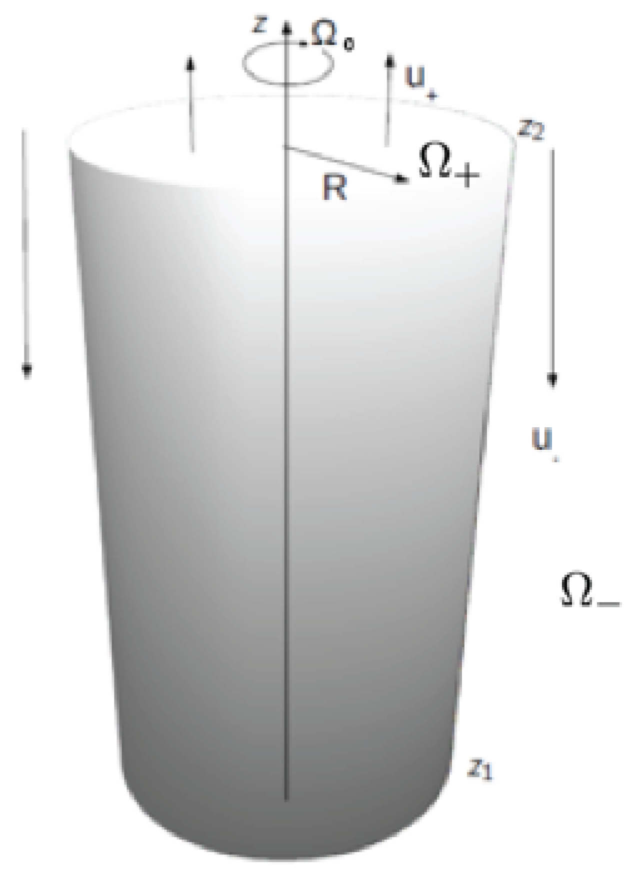
Figure 2.
Comparison of numerical solutions (solid lines) of the non-rotating dispersion relation given by Eq 26 for with the exact analytical values (open circles) given by Eq 27.
Figure 2.
Comparison of numerical solutions (solid lines) of the non-rotating dispersion relation given by Eq 26 for with the exact analytical values (open circles) given by Eq 27.
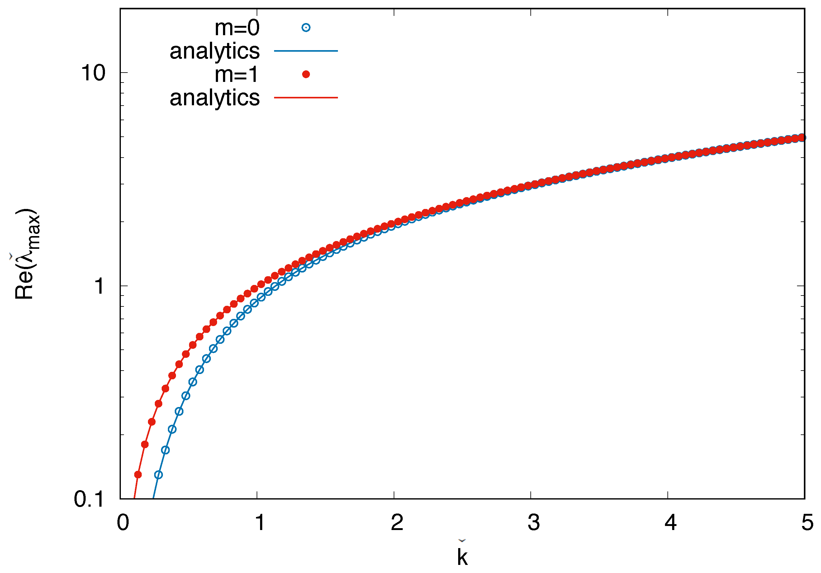
Figure 3.
Numerical solutions of the dispersion relation given by Eq 42 for varying values of m compared with the asymptotic expression for large (solid lines) given by Eq 43.
Figure 3.
Numerical solutions of the dispersion relation given by Eq 42 for varying values of m compared with the asymptotic expression for large (solid lines) given by Eq 43.
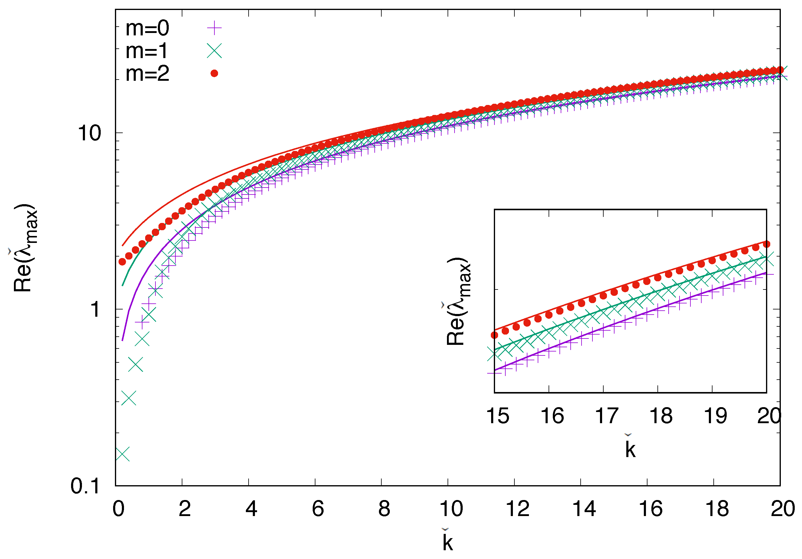
Figure 4.
Numerical solutions for fastest growing modes as function of the background rotation for varying values of m and two different vertical wavenumbers (left) and (right), compared with the analytic estimates (solid lines) for weak background rotation (solid lines) given by Eq 32.
Figure 4.
Numerical solutions for fastest growing modes as function of the background rotation for varying values of m and two different vertical wavenumbers (left) and (right), compared with the analytic estimates (solid lines) for weak background rotation (solid lines) given by Eq 32.
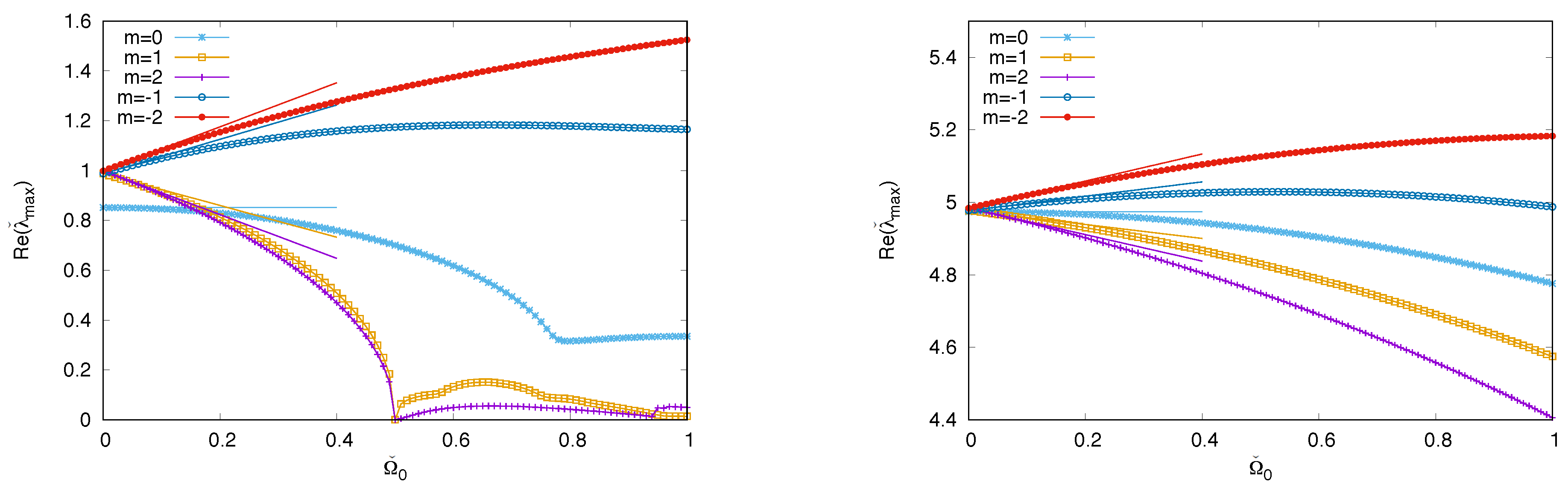
Figure 5.
Effect of rotation on the growth rates compared to the asymptotic results for low rotation rates (see Appendix A) for varying values of differential rotation (measured by ) as a function of the background rotation () for (left) and (right) and .
Figure 5.
Effect of rotation on the growth rates compared to the asymptotic results for low rotation rates (see Appendix A) for varying values of differential rotation (measured by ) as a function of the background rotation () for (left) and (right) and .
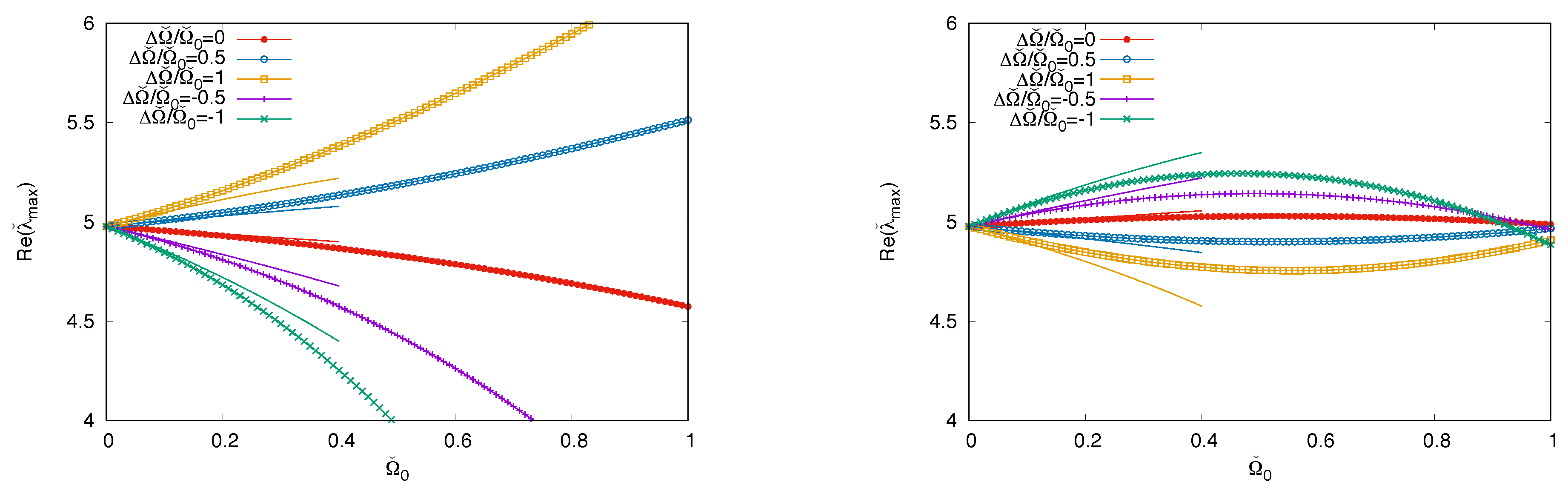
Figure 6.
Numerical solutions for the term in the angular momentum change expression given by Eq 56 (as calculated in Section 2.5) for (top panels) and (bottom panels).
Figure 6.
Numerical solutions for the term in the angular momentum change expression given by Eq 56 (as calculated in Section 2.5) for (top panels) and (bottom panels).
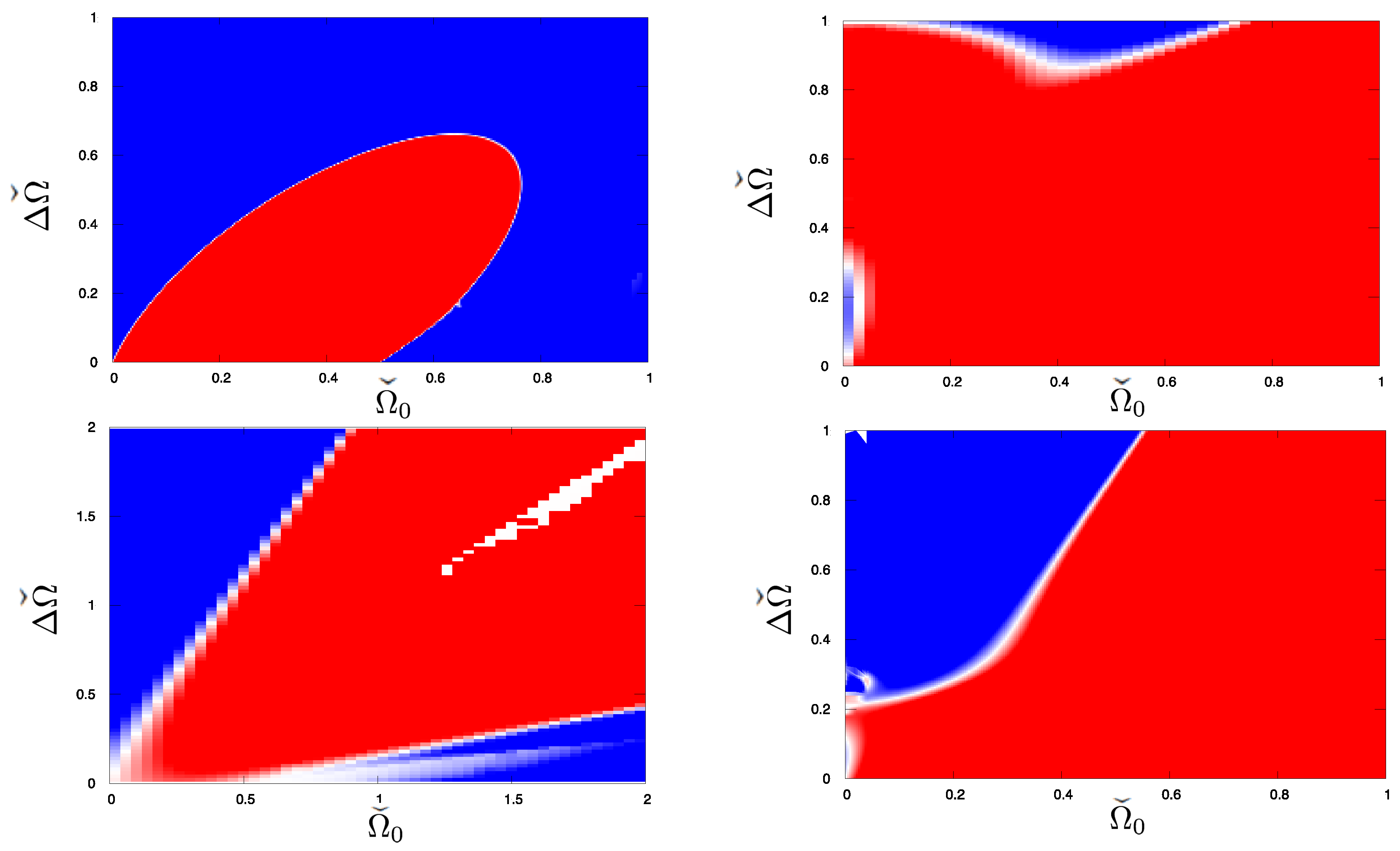
Figure 7.
Isocontours of vertical components of velocity field in the DNSs A2 (right) at , and A3 (left) at (see Table 1 for parameters and aspect ratio) showing the initial growth of the linear instability.
Figure 7.
Isocontours of vertical components of velocity field in the DNSs A2 (right) at , and A3 (left) at (see Table 1 for parameters and aspect ratio) showing the initial growth of the linear instability.
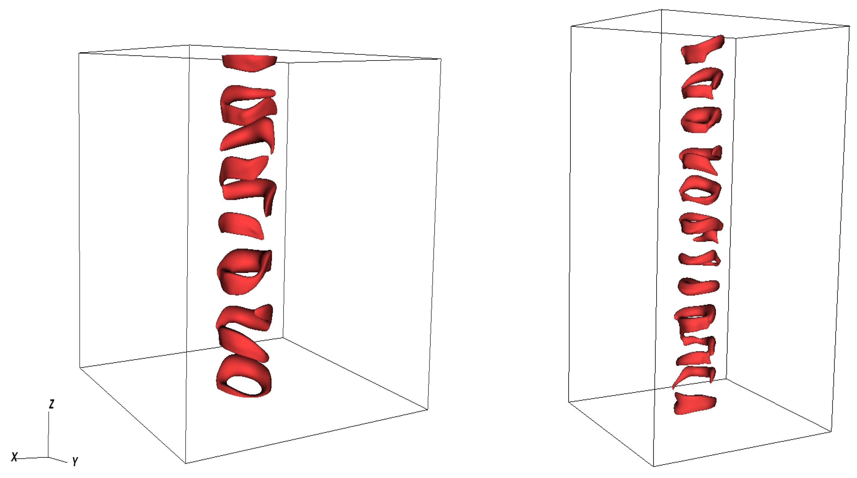
Figure 8.
Time evolution of the Reynolds stress term (left) and average angular velocity (left) for the DNS run A3 in Table 1.
Figure 8.
Time evolution of the Reynolds stress term (left) and average angular velocity (left) for the DNS run A3 in Table 1.
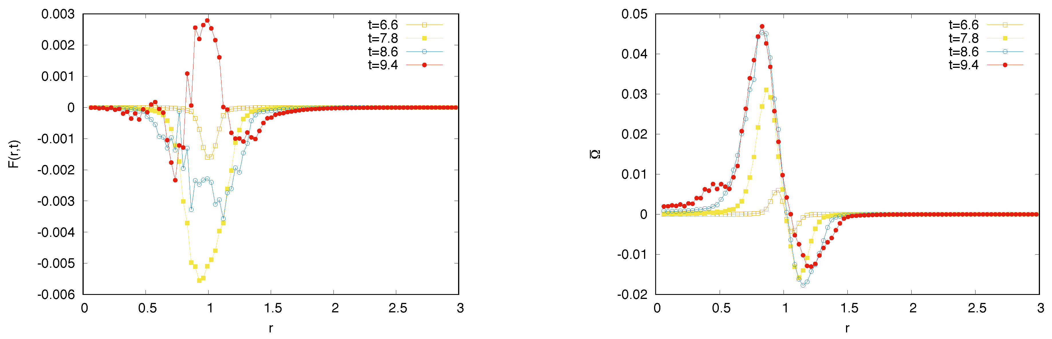
Figure 9.
Evolution of at early times for the DNSs A1 and A3.
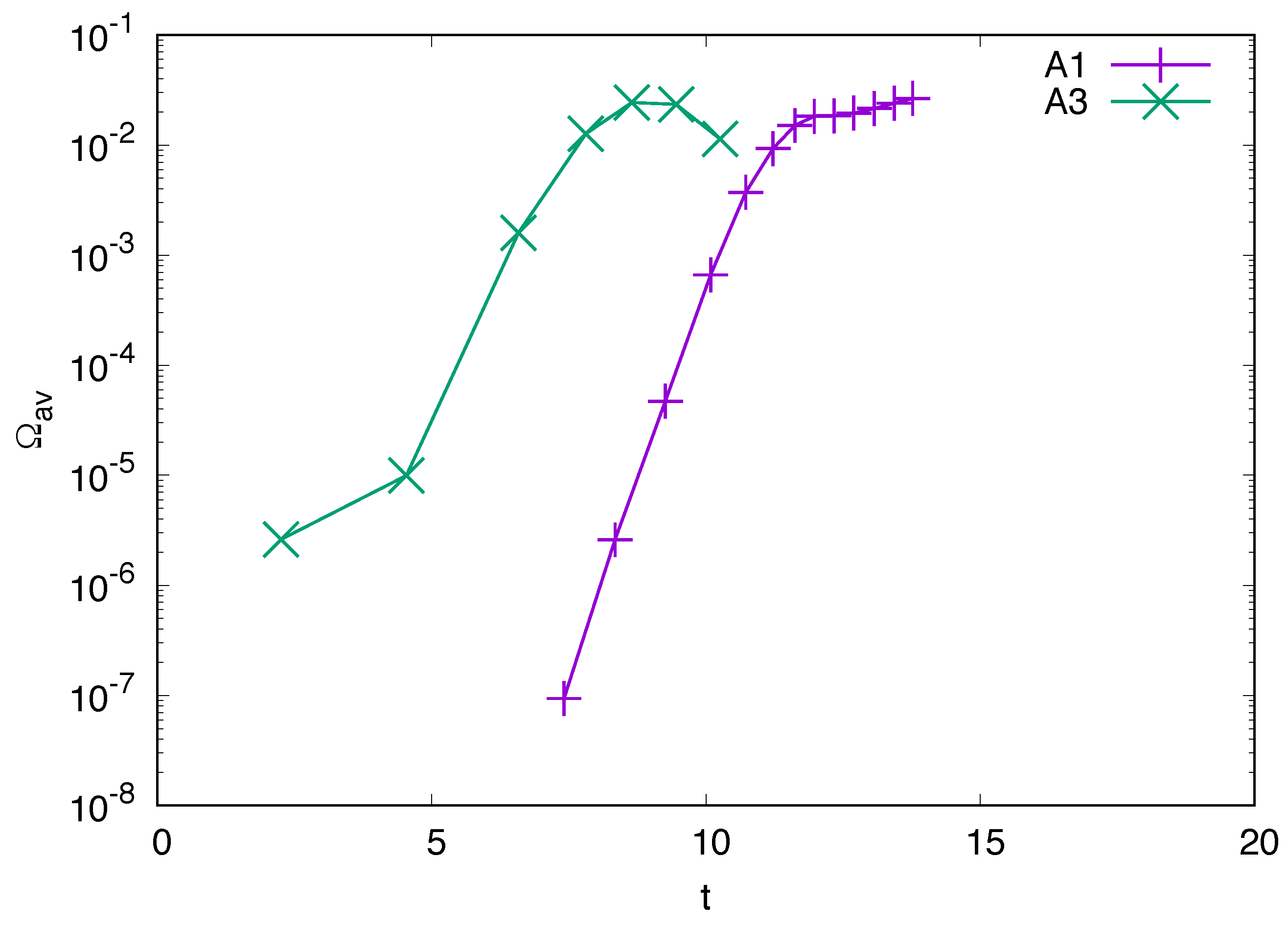
Figure 10.
Evolution of the angular momentum at early times for the , run.
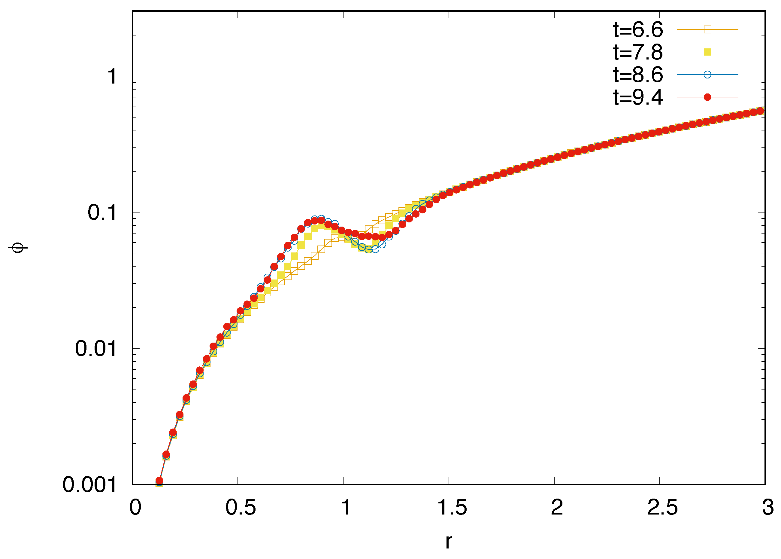
Figure 11.
Isocontours of vertical velocity for the DNS A3 at times and , showing the emergence of a helical flow pattern in the nonlinear phase.
Figure 11.
Isocontours of vertical velocity for the DNS A3 at times and , showing the emergence of a helical flow pattern in the nonlinear phase.
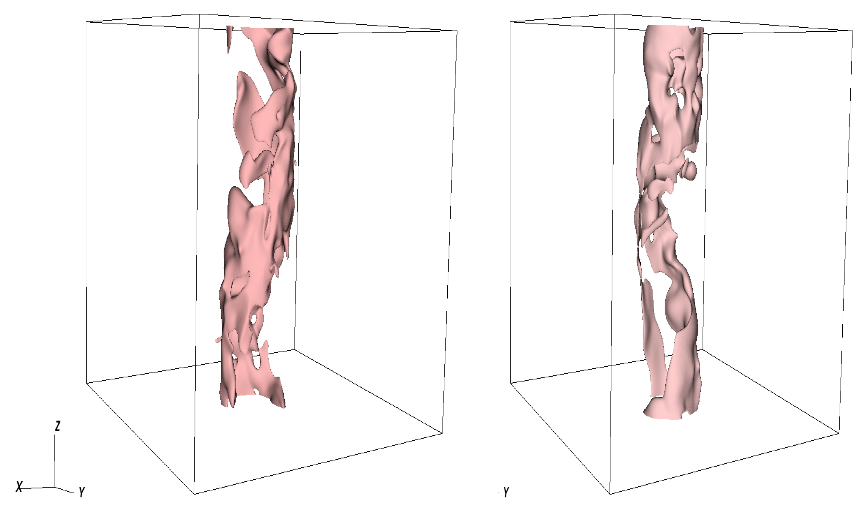
Figure 12.
Evolution of with time for the runs at and 625 illustrating the emergence of a helical tube.
Figure 12.
Evolution of with time for the runs at and 625 illustrating the emergence of a helical tube.
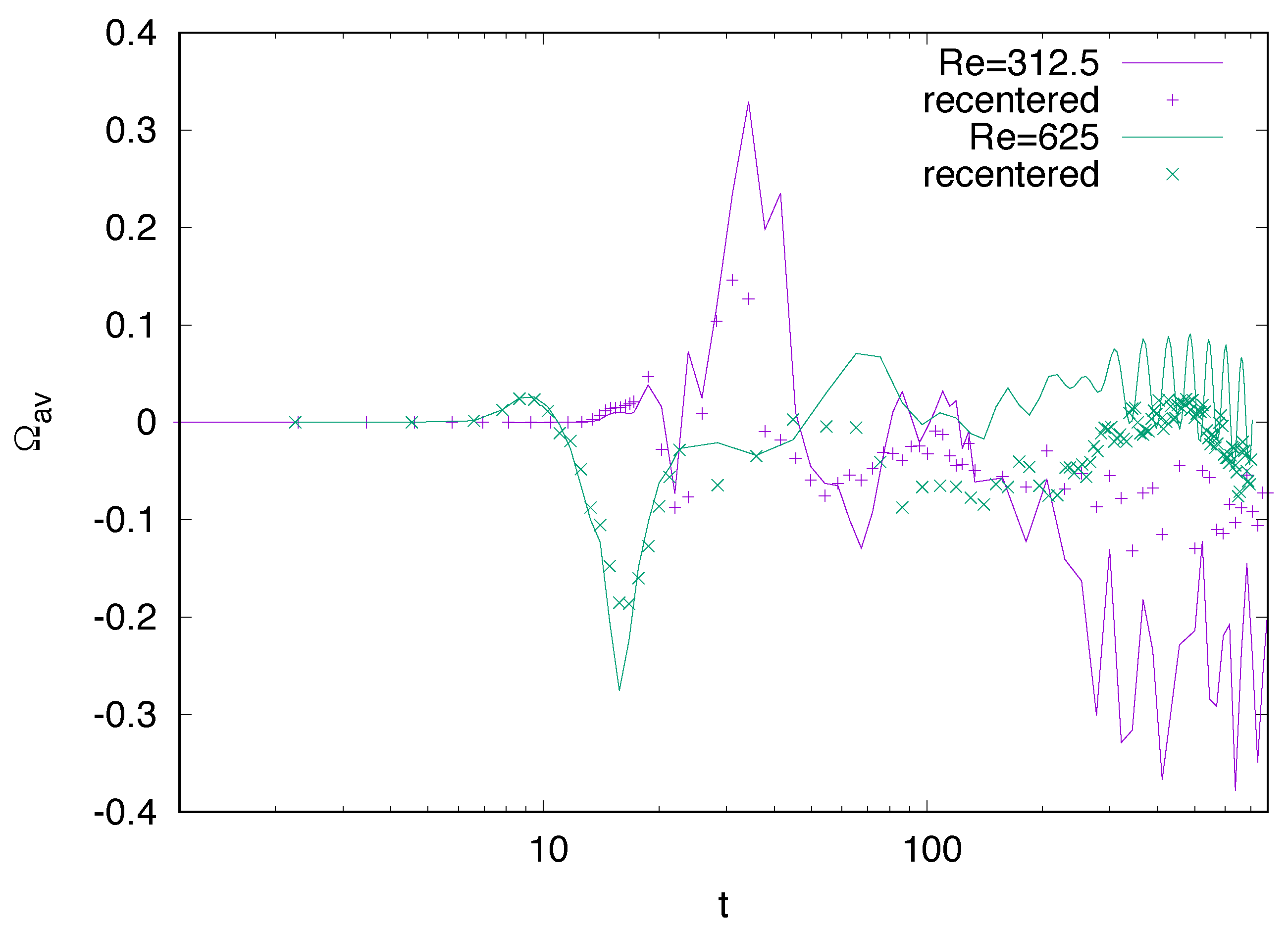
Figure 13.
Evolution of average rotation with time for the runs B1 and B2 (refer Table 1 ) showing early spin-down of the tube.
Figure 13.
Evolution of average rotation with time for the runs B1 and B2 (refer Table 1 ) showing early spin-down of the tube.
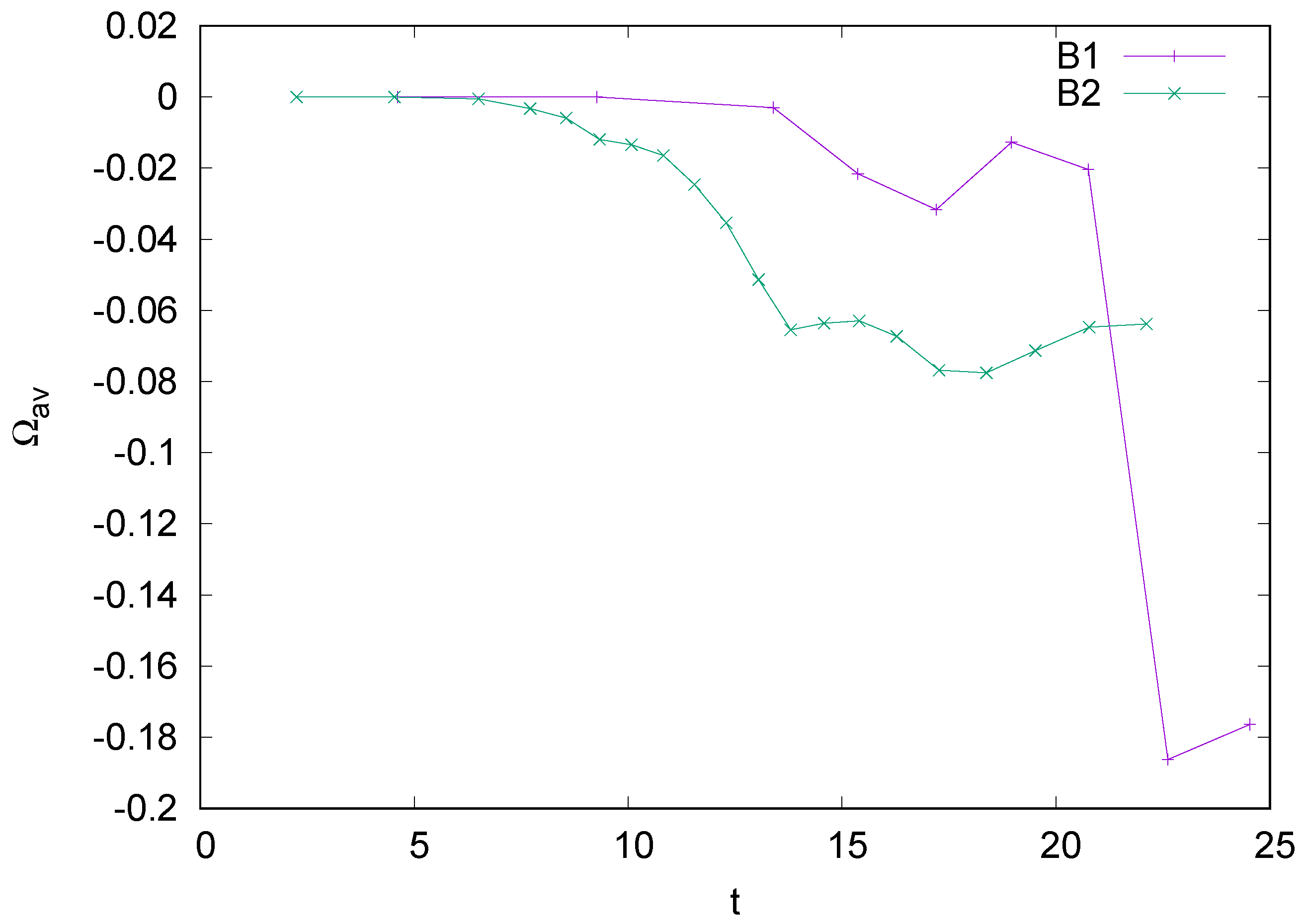
Figure 14.
Time evolution of the Reynolds stress term (left) and average angular velocity (right) for the DNS run B2 in Table 1.
Figure 14.
Time evolution of the Reynolds stress term (left) and average angular velocity (right) for the DNS run B2 in Table 1.
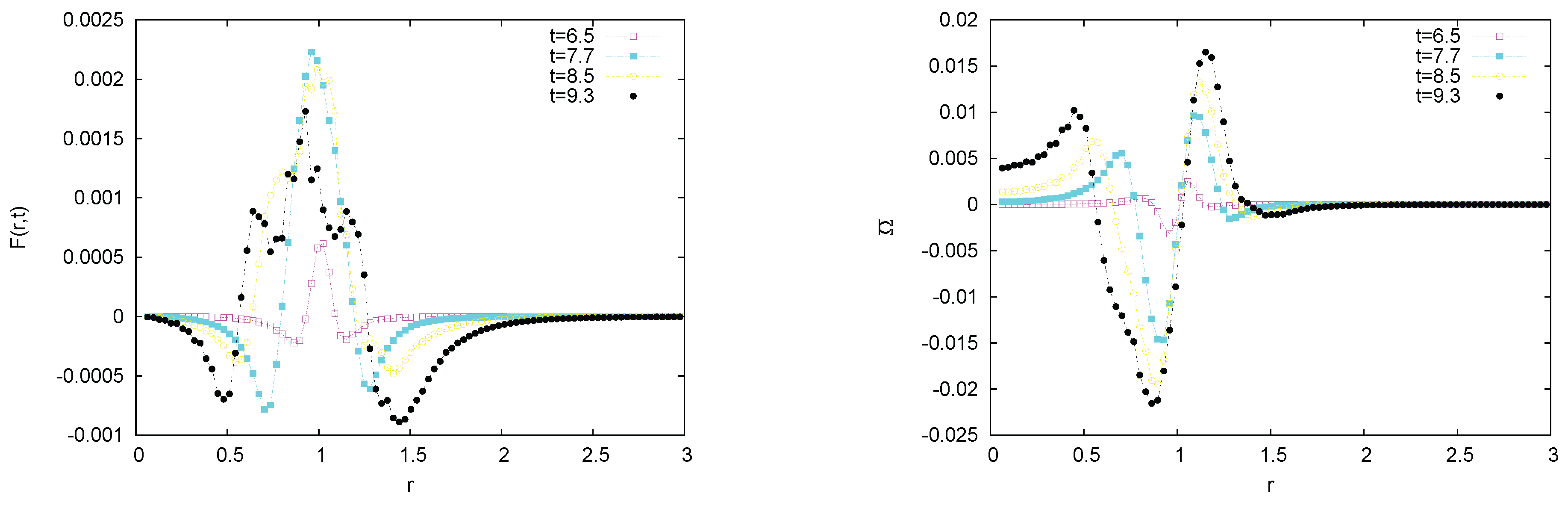
Figure 15.
The evolution of the averaged rotation rate for two sets of runs B3 and B4 (refer n Table 1 for details) illustrating the effect of domain size on the prediction of spin-up of the tube.
Figure 15.
The evolution of the averaged rotation rate for two sets of runs B3 and B4 (refer n Table 1 for details) illustrating the effect of domain size on the prediction of spin-up of the tube.
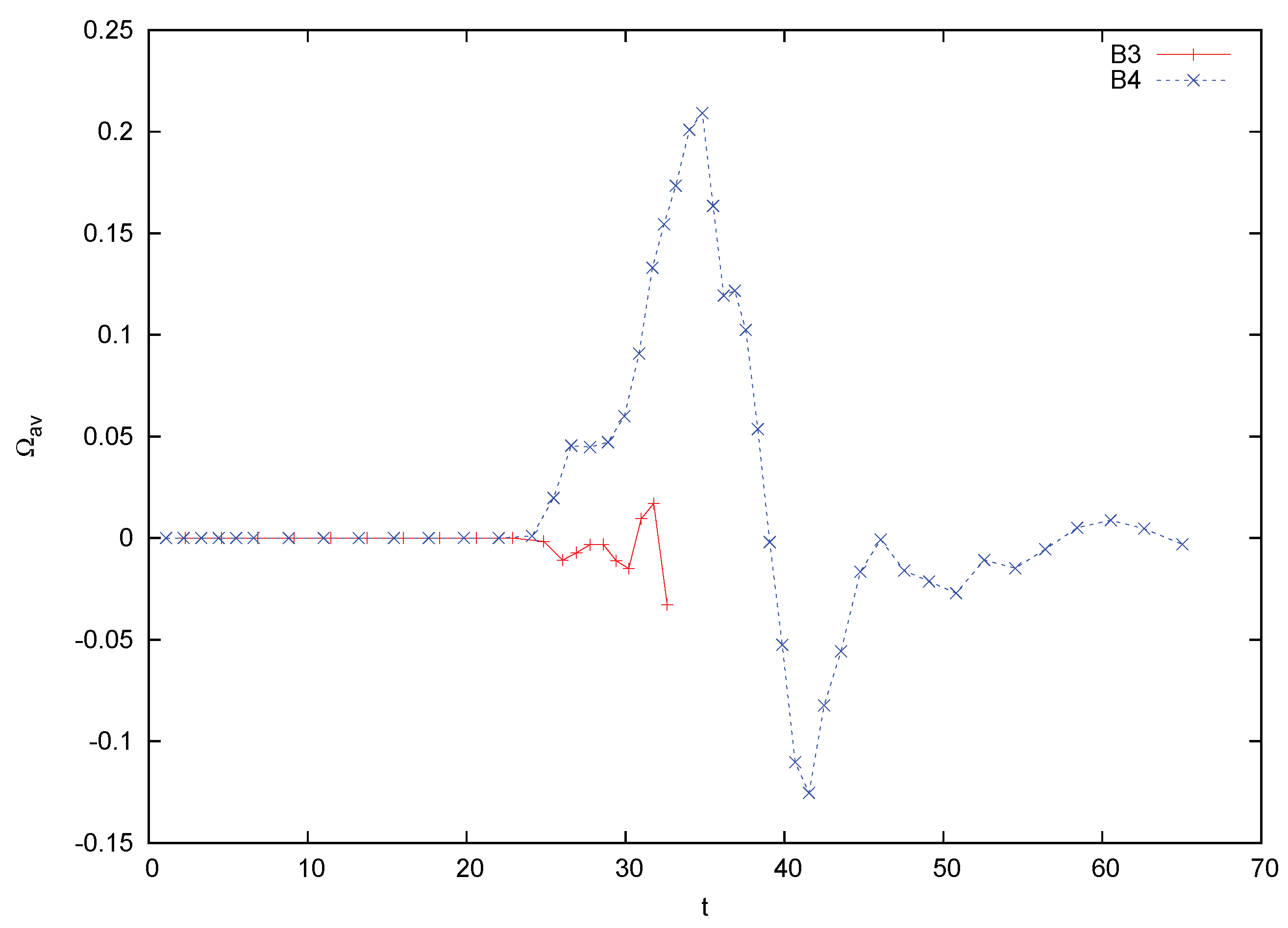

Table 1.
Properties of DNSs for varying values of parameters and problem setup/geometry
| Resolution | |||||
|---|---|---|---|---|---|
| A1 | 8 | 312.5 | |||
| A2 | |||||
| A3 | 625 | ||||
| B1 | 312.5 | ||||
| B2 | 625 | ||||
| B3 | |||||
| B4 | |||||
| B5 | |||||
| C1 | |||||
| C2 | 625 |
Disclaimer/Publisher’s Note: The statements, opinions and data contained in all publications are solely those of the individual author(s) and contributor(s) and not of MDPI and/or the editor(s). MDPI and/or the editor(s) disclaim responsibility for any injury to people or property resulting from any ideas, methods, instructions or products referred to in the content. |
© 2026 by the authors. Licensee MDPI, Basel, Switzerland. This article is an open access article distributed under the terms and conditions of the Creative Commons Attribution (CC BY) license (http://creativecommons.org/licenses/by/4.0/).
Copyright: This open access article is published under a Creative Commons CC BY 4.0 license, which permit the free download, distribution, and reuse, provided that the author and preprint are cited in any reuse.


