
Submitted:
23 January 2026
Posted:
27 January 2026
You are already at the latest version
Abstract
Efficient heat recuperation is one of the crucial aspects affecting the performance of mixed-refrigerant Joule-Thomson (MR JT) cryocoolers. This becomes even more important in the case of precooled systems which improves the performance, but on the other hand, emphasizes the challenges related to the effectiveness of the recuperation process. Modelling of recuperation process is challenging itself as recuperation concerns both gaseous, liquid phases and two-phase flow. Moreover, application of mixed-refrigerant brings a lot complexity to the modelling of MR thermo-hydraulic properties. At last, experimental validation of modelling results requires very sophisticated measurement setup especially in terms of mixed-refrigerant composition which can significantly differ from charged proportions. This paper present modelling approach of complete two-phase recuperation heat transfer process. In total, 96 correlations combinations were examined. The results are compared with the experimental results achieved using novel validated method of noninvasive, continuous method of determining composition. Carried modelling validated with experimental results provides useful insight concerning heat transfer phenomena in recuperation section of MR JT cryocoolers or other mixed-refrigerant based systems.
Keywords:
recuperation heat transfer
; mixed refrigerant
; experimental study
; numerical modelling
; precooled MR JT
; statistical analysis
1. Introduction
Recuperative heat transfer is one of the key elements influencing the performance of mixed-refrigerant Joule-Thomson (MR JT) cryocoolers, used to obtain low temperatures in the cryogenic range and often deployed due to their simplicity, which results in high reliability. Therefore, in order to avoid undesirable heat transfer scenarios, such as the presence of pinch points, an accurate and robust modeling framework utilizing single- and two-phase heat transfer correlations needs to be developed. Additionally, modeling results must be validated with trustful experimental data, especially in terms of mixed-refrigerant composition.
Due to their low cost, high reliability, wide capacity range and suitable operational range, brazed plate heat exchangers (BPHE) have become widely used in MR JT cryocoolers [1,2]. Effective recuperation usually requires the application of a few BPHE units in series [1,2], which provides sufficient thermal length. However, it can trigger issues related to two-phase flow, especially at the heat exchanger inlet ports. Currently, data on heat transfer effectiveness during recuperation in MR JT cryocoolers using BPHE is limited, especially for systems with precooling [1,3]. Precooled MR JT cryocoolers have been reported to be more efficient than single-stage MR JT systems, but also more demanding in terms of heat transfer effectiveness in the recuperation section [4].
The authors of [2] realized an experimental survey on the recuperation heat transfer performance of middle BPHE (second out of 3 BPHEs connected in series) and validated it against developed model. The LMTD-based model takes into account numerous boiling and condensation heat transfer correlations specifically for pure refrigerants. In total, 40 correlation combinations were tested, of which the authors recommended two which agree +- 30% with the experimental data. The error in the composition of the circulating MR is reported as +-4.3%, but it is not clear how it affects the validation procedure. It is also not clear how often and when exactly the circulating MR composition was measured. This information is crucial as it was recently shown by [5] that the composition of circulating MR varies significantly with thermal load or the progress of the cooldown process.
The modeling of complete recuperation heat transfer process for tube-in-tube heat exchanger is presented in[6]. The authors did not consider different boiling and condensation correlations. The modeling results were validated against the experimental data; however, it is reported that the circulating MR composition was not always measured, and it was assumed to be the same as the charged one. The measurement error of the MR composition is not reported.
While [2,6] has investigated the MR of hydrocarbons, the work of [7] is focused on the argon-freon MRs. The recuperator was a customized microchannel heat exchanger (MCHE). The application of MCHE allows one to minimize the MR charge, which, in general, is desired but makes the system sensitive to probing [5]. The authors validated the LMTD-based model against the experimental data. Gas chromatography was used to measure the MR composition; however, it is stated that it was used to confirm charged compositions, which will likely differ from the circulating one. The authors examined 8 condensation and 8 evaporation heat transfer correlations .
Tests in the section incorporated into the dedicated test stand, including the GM cryocooler, have been performed in [8]. Such an approach enabled to precisely simulate the conditions of MR in the test section but, on the other hand, limited the measurement to flow boiling phenomena. The authors compared experimental data with two single-phase correlations that reported significant deviations for qualities ranging from 0.4 to 0.8. The study focused on MRs consisting of nitrogen and hydrocarbons. Circulating MR composition was frequently measured via gas chromatography.
Experimental tests aimed at obtaining the thermodynamic and hydraulic behavior of the tube-in-tube heat exchanger have been performed in [9]. The authors measured the composition of the MR, consisting of R14, methane, ethane, propane, isobutane, isopentane, nitrogen and neon, as well as temperatures and pressures along the HX. The heat transfer characteristics of the heat exchanger were concluded to be very sensitive to the mixture used, which means that circulating MR composition measurement is crucial for reliable modeling of this heat transfer case. The works of [10,11] led to very similar conclusions for tube-in-tube HX and MR consisting of nitrogen and hydrocarbons.
The most questionable point of most studies is the measurement and later consideration of circulating MR composition. The available studies do not address the topic of the exact measurement moment, which according to recent findings from [5], significantly affects the measured circulating MR composition. Secondly, most studies report measurement errors related to MR composition, but without considering the impact of this issue on the results, even if a significant impact of MR composition was concluded [9].
Successful validation of the modeling results requires complete information concerning heat transfer conditions, including the circulating composition of the mixed refrigerant. According to numerous works, it cannot be simply determined based on the charge composition of the mixed refrigerant [3,9,11,12,13,14,15] and will depend greatly on the specific operational conditions and architecture of the system. Credible validation would require many measurements of the MR composition during the test and in case of application of the invasive method (requiring probing of the MR sample for further investigation ) will affect the remaining MR composition [5]. To solve this issue, the following study employed a novel noninvasive method to measure MR composition that is described in detail in [5]. Moreover, it was investigated how uncertainties of the MR composition measurement affect the credibility of results, which was not performed in any of the studies cited above.
In this work, a series of measurements were performed on MR JT cryocooler, using binary mixtures of methane and ethane in various concentrations. Inlet temperatures for the low pressure and high pressure streams, obtained in recuperation section measurements of the system, were used as input to the proposed numerical model, which utilizes the e-NTU method and produces a temperature distribution along the heat exchanger length as an output. A wide variety of single- and two-phase correlations for ideal heat transfer were investigated. Selected correlations were also used with available correction factors taken into account to further improve computational accuracy. All results were compared with the experimental data and evaluated.
2. Test Stand
The experimental study was performed using the precooled MR JT cryocooler located in the Laboratory of Cryogenics and Gas Technology at Wroclaw University of Science and Technology. A detailed description of the test stand is provided in [1] while the Process and Instrumentation Diagram (P&ID) is presented in Figure 1, respectively. The study was carried out using the instrumentation listed in Table 1.
The study focuses on the recuperation heat transfer that takes place in the cold box which is presented in Figure 2. The cold box contains the precooler HX2 that thermally couples MR and precooling cycles, three BPHE recuperators connected in series HX3, HX4, HX5, the CV1 control valve, and the electric heater EH. In addition, there are numerous temperature sensors (T4 - T12) and pressure sensing ports (SeV2 - SeV10) which are also used for differential pressure measurements. In operation, the empty spaces inside the cold box are tightly filled with thermal wool sheets, enclosed by a front XPS sheet.
The composition of the binary gas mixture was determined using the method described by [5]. The density measurement system was calibrated over the range kg m−3, yielding a combined standard uncertainty of the calibrated density measurements of kg m−3. The corresponding expanded uncertainty () of density for the data used in this study ranged from to kg m−3 (mean kg m−3). The expanded uncertainty (k=2) of the inferred composition ranged from to mol% (percentage points), with a mean value of 8.47 mol%.
3. Experimental Study
Each dataset in this study was obtained from a stand-alone experiment. Between successive cooldowns, at least 12-hour interval was maintained to let the system warm up, ensuring that each cooldown started from a uniformly heated baseline. A single measurement took approximately 10 h to complete; data were analyzed over the final 5 h 14 min on average, after the system had reached steady operation. An example of sensor readings during cooldown and stabilization is shown in Figure 3.
The experiments were conducted at fixed discharge pressures (P2, Figure 1) and suction pressures (P1, Figure 1) of the MR compressor (C1, Figure 1), with constant electric heater power (EH, Figure 1). The precooling temperature (T4, Figure 1) was not directly controlled; instead, the frequency of the precooling compressor (C2, Figure 1) was adjusted. Measurements were performed for two different MR charges in the system; in both cases, the circulating MR composition was monitored continuously throughout each experiment. The design-of-experiments matrix is summarized in Table 2.
4. Numerical Model
A steady-state numerical model was formulated to predict the outlet temperatures in a brazed plate heat exchanger assembly when all inlet conditions are known. Three plate heat exchangers operating in series were represented as a single equivalent HX. Within each HX, the physical stack of plates was simplified to one plate channel whose heat transfer area is equal to the total exchange surface. The model does not take the pressure drop along the HXs into account.
Figure 4.
Numerical model - discretization scheme. (a) HX geometry simplification (b) Temperatures used by the model (one cell).
Figure 4.
Numerical model - discretization scheme. (a) HX geometry simplification (b) Temperatures used by the model (one cell).
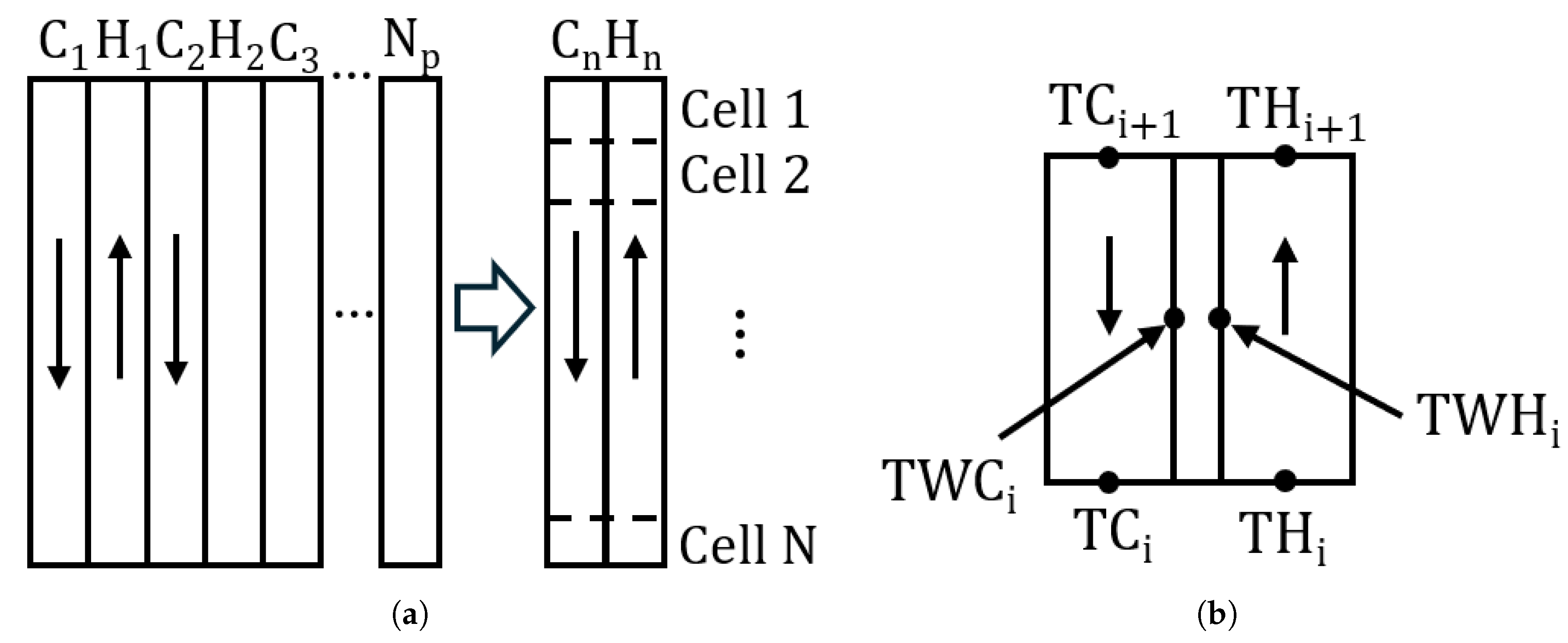
The equivalent surface of HX was divided along the length of the HX into N computational elements (cells) of equal area, for . An initial guess for the temperature distribution of both streams was provided. The number of cells in this study is set to after an investigation of mesh sensitivity has been performed. The difference in total power of the heat exchanger Q between 400 and 800 cells was, on average, 1%. The initial temperature distribution was assumed to be linear, with the difference between the inlet and outlet for both channels set at 5 K. The outlet of element i served as the inlet of element .
The block diagram of the numerical model is shown in Figure 5. After the initial conditions were defined and heat transfer correlations selected for a particular case, the local properties of the working fluid mixtures were obtained from REFPROP 10 [16]. For each element i, quantities such as heat capacity , density , viscosity , and thermal conductivity k were obtained for both hot and cold streams in the cells. The properties in one element are calculated for the inlet of the cell. In the case of the two-phase regime, vapor quality is used to obtain estimated properties using Eq. 1. Heat transfer was computed for each cell using the effectiveness-NTU method. Heat capacity rates were formed for both streams (Eq. 2), and then the minimum and maximum capacity rates were found, (Eq. 3 and 4). The NTU per element was consequently calculated (Eq. 5), where denotes the local overall heat transfer coefficient. The effectiveness of the heat exchanger was then obtained from the for the BPHE counter-flow arrangement. Lastly, using Eq. 6, temperatures were updated using the energy balance for both streams and all cells (Eq. 7). The iteration error for one cell was defined as the relative difference between the new (k+1) and old (k) temperature values (Eq. 8). The global error is expressed as the average error in all cells. The solving process was completed when , where the tolerance was .
5. Results and Discussion
Temperature, pressure, and mass flow measurements were performed in the recuperation section of the MR JT cooler while operating in a two-phase regime. Experimental data (input temperatures, pressures, composition and mass flow) were used as input to model the heat transfer in the recuperation section using heat transfer correlation sets. Additionally, calculations for all data points were performed for the range of possible mixture compositions, i.e. percentage points from the measured value, with an increment of one percentage point. In this range, the composition with the lowest error for the considered case is selected and used for further analysis. This is later referred to as "composition correction", not to be confused with the evaporation correction of the heat transfer coefficient.
There were 22 data points from the experiment. Taking into account the 15 possible mixture compositions and 96 correlation combinations in total, this yields a total of 31680 computational cases. Correlations used are presented in Table 3.
It is important to note that the plots in Figure 12, Figure 13, Figure 14, Figure 11, Figure 10 and Figure 15 have a logarithmic scale of point density to capture both high point concentrations and outliers. All data points have been mapped on the 2D histogram, and the data range has been established to be 135 to 245 K for both axes. This range was then divided into 30 bins, and based on the point count per bin, the density map was created for the data subsets used in small scale comparisons and the overall results.
In this study, the main error definition used is MAE (Mean Absolute Error). Detailed statistical analysis can be found later in this chapter.
Due to the high number of correlation combinations (96) and the wide range of possible mixture compositions (15 percentage points), the calculated temperature distributions in some considered cases exhibit the lowest error for the measured values, while in other instances, the lowest error is achieved for minimum values, and in some cases the lowest error is achieved for the maximum possible concentration values, as shown in Figure 7, Figure 8, and Figure 9. This observation emphasizes the importance of the discussion regarding the impact of mixture composition on results in similar studies, especially with binary mixtures that differ significantly in boiling points; this effect may not be as pronounced with mixtures that have more components. [11]
Figure 6 shows the exemplary temperature distributions for the overall best pair of correlations and the effect of composition correction. In Figure 6a, the results for the measured mixture composition are presented. Figure 6b shows the temperature distribution for the corrected composition; in this case, the methane concentration is decreased by 7 percentage points. As a result, the error decreased from 57.1 K to 7.64 K.
A comparison of the corrected and uncorrected cases is presented in Figure 10, and their distribution in Table 4. The majority (73.9%) of all modeling results before composition correction were within a range of ±30% of experimental values, 59.3% in the range of ±20% and 36.3% within ±10% of experimental values. After the composition correction, these values increased to 84.4%, 75.9% and 58.9%, respectively. Overall, the two-phase heat transfer coefficients ranged from 0.13 to 2.90 for evaporation with correction, and 0.585 to 36.1 for evaporation without correction. The condensation heat transfer coefficient values ranged from 0.36 to 8.17 . Single phase heat transfer, depending on the phase, ranged from 1.77 to 8.71 for the liquid phase and from 0.53 to 17.8 for the vapor phase. The combination of correlations with the lowest overall error was Kuo for condensation, Hsieh and Lin for evaporation with the Fujita correction factor, and Wanniarachchi for single phase heat transfer.
A high concentration of points can be observed in the range of model data from 220 to 240 K and from 145 to 190 K for experimental temperatures (referred to as high error band in Table 5 and Table 4) visible in Figure 10c,d. This area is likely the source of high error values in the overall results, since when all correlation combinations are taken into account, the composition correction decreases the percentage of points in this zone from 29.7% of all points to 15.1%. The number of outliers (single points or small concentrations of points with high error values) is also significantly decreased, as the number of points outside the -20% range decreased from 3.6% to 0.38% of data points. The number of points beyond the 20% range decreases from 38.4% to 22.5%. Considering the top 15 combinations temperature map in Figure 10a,b, composition correction decreased the number of points in the high error band from 13.6% to 2.7% of all data points, reduced the number of points outside the -20% range from 1.85% to 1.55%, and resulted in a decrease in the overall number of points in the ranges of ±30% (84.6% vs 92.5%), ±20% (73.3% vs 88.4%), and ±10% (45.5% vs 66.6%). Compared to the overall results, the percentage of high error points is very small for the top 15, and the distribution is more symmetrical.
The composition correction results in an analogous change in one correlation, as shown in Figure 11 and Table 5, where the chosen Hsieh & Lin evaporation correlation results, both without and with composition correction, are compared. Consequently, this yields an increased overall amount of points in the ranges of ±30% (76.7% vs 87.3%), ±20% (62.5% vs 79.2%), and ±10% (37.7% vs 60.8%), as well as a reduction in the number of points in the high error band (26.3% vs 11.6%).
Figure 12 shows the comparison between the experimental and modeled outlet temperature data after the composition correction for two selected pairs of condensation correlations, chosen based on the lowest and highest error values: Kuo and Thonon, respectively. In Figure 12c,d, the 220-240 K model temperature band contains a significant portion of all points, i.e., 10% for Kuo and 17% for Thonon, similar to the previous comparisons. There are significant differences in data distribution between Kuo and Thonon in ranges: ±30% (88.9% vs 82.7%), ±20% (82.1% vs 73.5%), and ±10% (62.4% vs 56.8%), as well as a reduction in the number of points in the high error band (26.3% vs 11.6%). As shown in Figure 12a, the high error band is much less discernible if the analyzed correlation combinations have a lower overall error value, as in this instance where the top 5 is taken into account; In the case of the top 5, the high error band contains 2.5% and 7.2% of the data points, and the point distribution changed as follows: range of ±30% (92.5% vs 90.6%), ±20% (89.3% vs 83.6%), and ±10% (67.3% vs 63.8%). Kuo condensation also exhibited the highest spread of values among all the condensation correlations, with HTC values going as low as 0.355 , while the others had their lowest values in the order of 4 .
Analogous observations can be made regarding the correlations of evaporation with low and high error values. In Figure 13, two evaporation correlations are compared in the same manner as in Figure 12. Considering the overall results, 11.6% of points for Hsieh & Lin and 18.5% for Han fall within the high error band. A noticeable gap in the 10-30% range for experimental temperature values from 160 K to 190 K can be observed. The overall distribution of points for Hsieh & Lin and Han is as follows: range of ±30% (87.3% vs 81.5%), ±20% (79.2% vs 72.6%), and ±10% (60.8% vs 56.9%). For the top 10 correlation combinations, the distribution is: range of ±30% (92.3% vs 88.9%), ±20% (88.1% vs 82.5%), and ±10% (66.8% vs 64.0%).
Evaporation correction also seems to have the most significant effect on the results. In Figure 14, a comparison between uncorrected and corrected evaporation heat transfer is presented. The overall distribution is as follows: range of ±30% (90.9% vs 78.9%), ±20% (83.1% vs 68.9%), and ±10% (63.0% vs 52.9%); for the top 10: range of ±30% (92.7% vs 81.8%), ±20% (88.2% vs 71.7%), and ±10% (66.8% vs 56.1%). In the high error band, overall there are 7.35% and 22.6% of all points, and for the top 10 combinations, the distribution is 2.6% and 22.6%, respectively. Interestingly, evaporation correction increases the percentage of points in the high error band the most among all the comparisons presented.
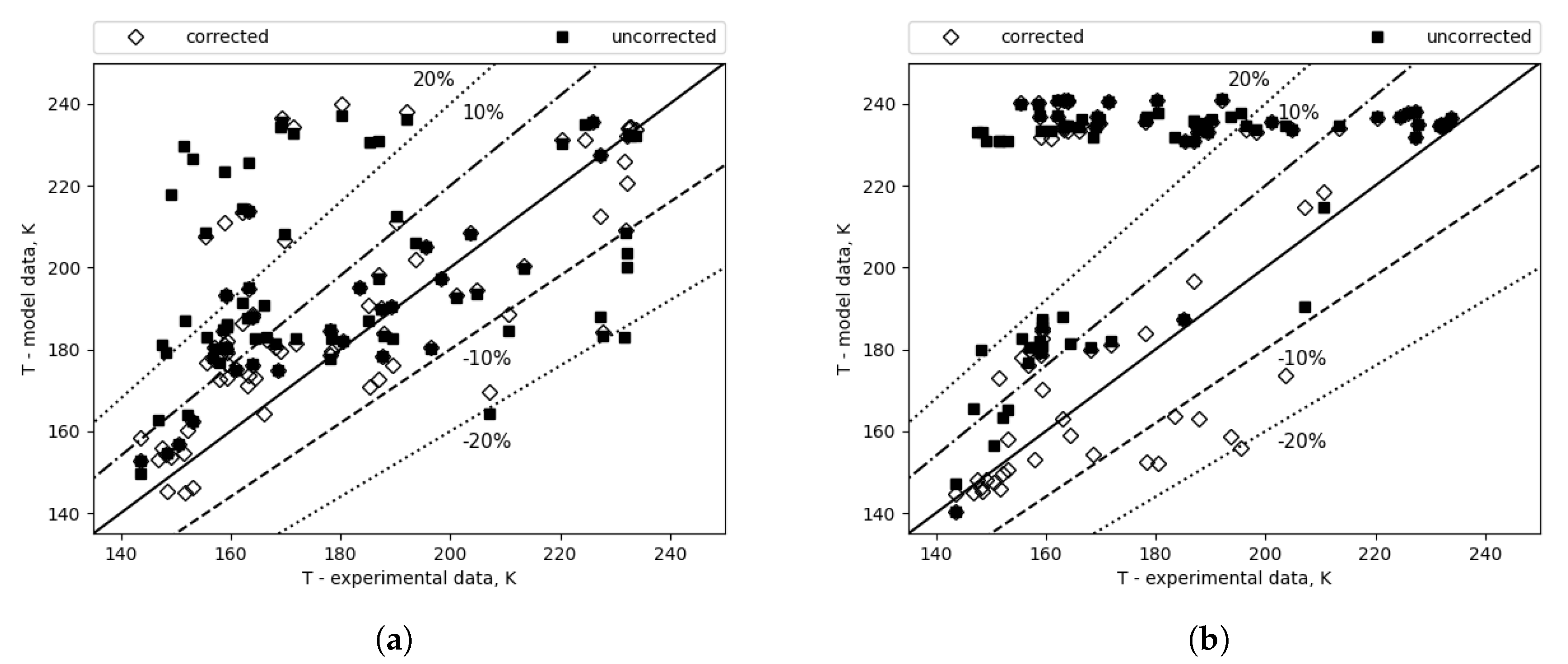
Correction seems to have less of an effect if the correlation combination itself has a low error, as shown in Figure 15, which depicts the comparison of outlet temperatures for the combination with the lowest calculated error (Figure 15a) and the highest (Figure 15b). In the case of the combination with the highest error, the correction yielded approximately a 40 K reduction in error, and for the best overall combination, the composition correction resulted in approximately a 5 K decrease.
The cause of the high error band, or more broadly speaking, the strong asymmetry in the distribution of model temperatures, is most likely due to a general overestimation of the overall heat transfer coefficient values in this study. An example can be seen in Figure 6a.
The assumption of no pressure drop may influence the results by shifting the phase change temperatures, especially in the cold stream, where a pressure drop of 0.2 bar can change the evaporation temperature by 3 K. However, the impact of the composition range is substantial (an 8 K change) and will not be negated by the introduction of pressure drop to the analysis.
Figure 6.
Temperature distribution along the HX length for the overall best combination of correlations. Single phase: Wanniarachchi, condensation: Kuo, evaporation: Hsieh & Lin and no evaporation correction. (a) MR composition as measured.(b) Corrected composition.
Figure 6.
Temperature distribution along the HX length for the overall best combination of correlations. Single phase: Wanniarachchi, condensation: Kuo, evaporation: Hsieh & Lin and no evaporation correction. (a) MR composition as measured.(b) Corrected composition.
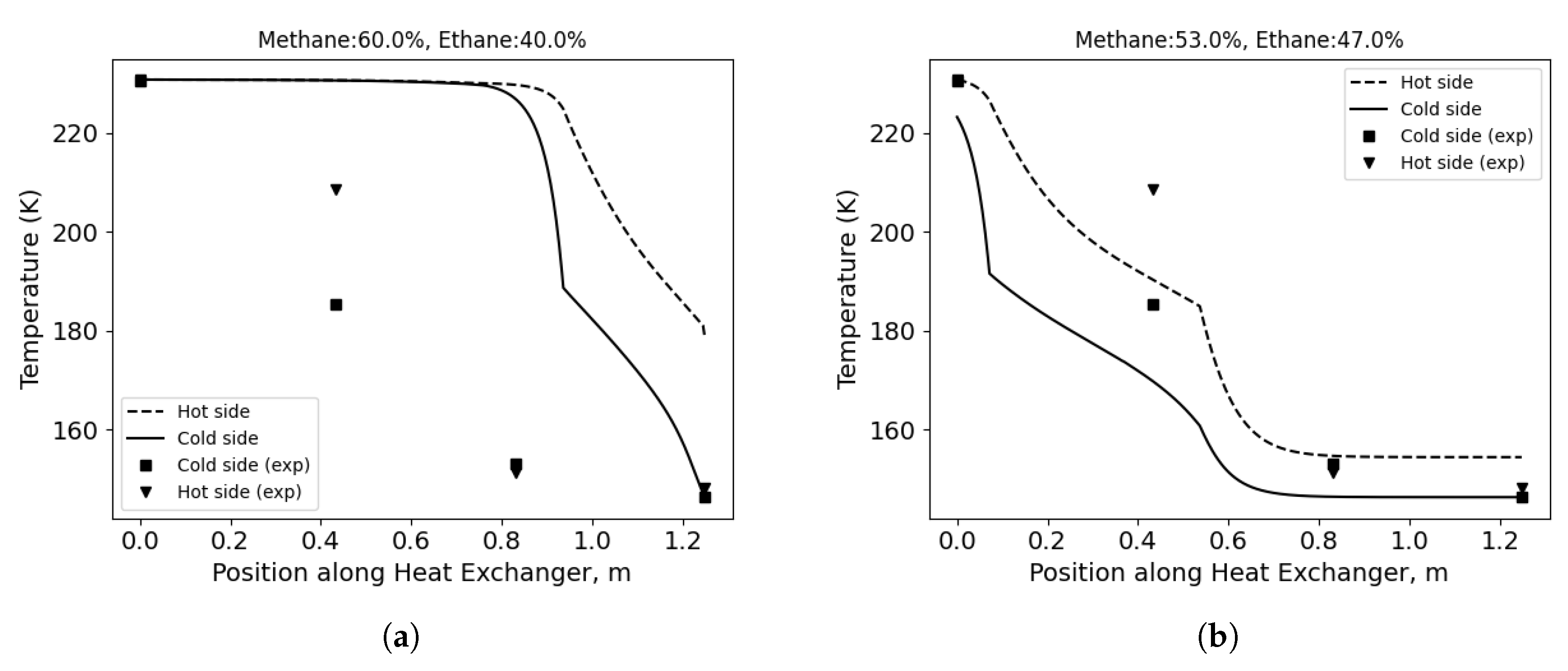
Figure 7.
Temperature distributions along the HX length for minimum, maximum and measured composition of the MR. Best fit for minimum possible methane concentration. (a) Cold side. (b) Hot side.
Figure 7.
Temperature distributions along the HX length for minimum, maximum and measured composition of the MR. Best fit for minimum possible methane concentration. (a) Cold side. (b) Hot side.
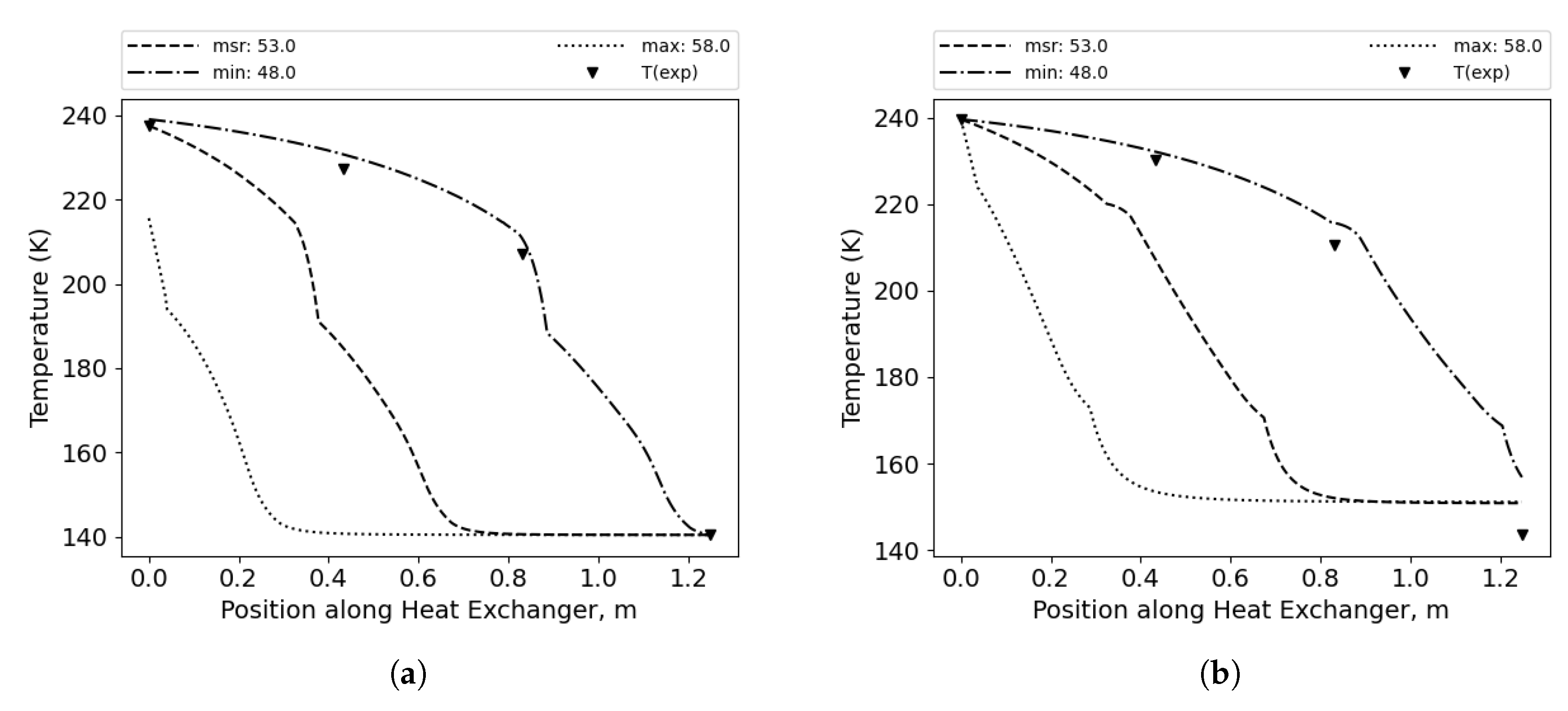
Figure 8.
Temperature distributions along the HX length for minimum, maximum and measured composition of the MR. Best fit for measured methane concentration. (a) Cold side. (b) Hot side.
Figure 8.
Temperature distributions along the HX length for minimum, maximum and measured composition of the MR. Best fit for measured methane concentration. (a) Cold side. (b) Hot side.
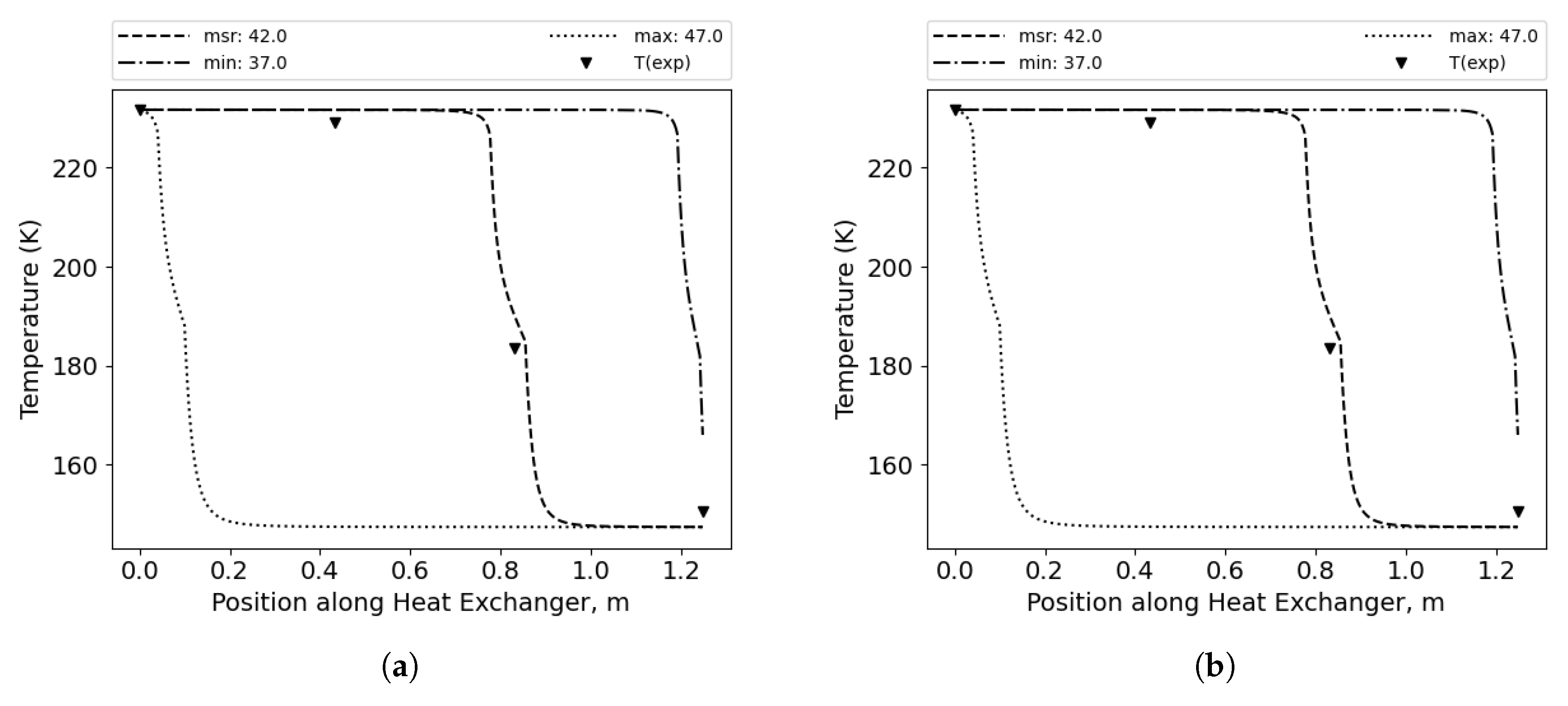
Figure 9.
Temperature distributions along the HX length for minimum, maximum and measured composition of the MR. Best fit for measured methane concentration. (a) Cold side. (b) Hot side.
Figure 9.
Temperature distributions along the HX length for minimum, maximum and measured composition of the MR. Best fit for measured methane concentration. (a) Cold side. (b) Hot side.
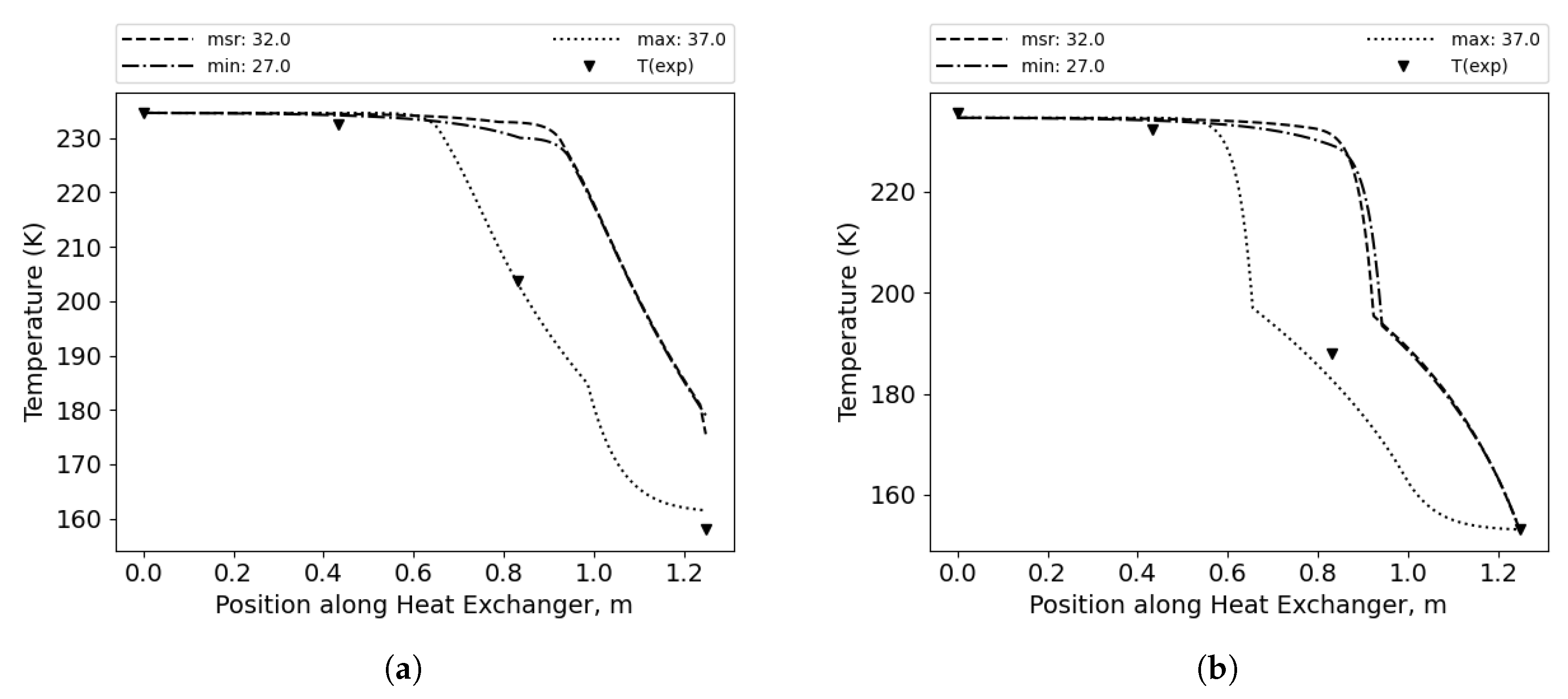
Figure 10.
Outlet temperature comparison for all cases and combinations - composition corrected vs as measured. (a) Corrected cases - top 15. (b) Cases with composition as measured - top 15. (c) Composition corrected cases - overall (top 96). (d) Cases with composition as measured - overall (top 96).
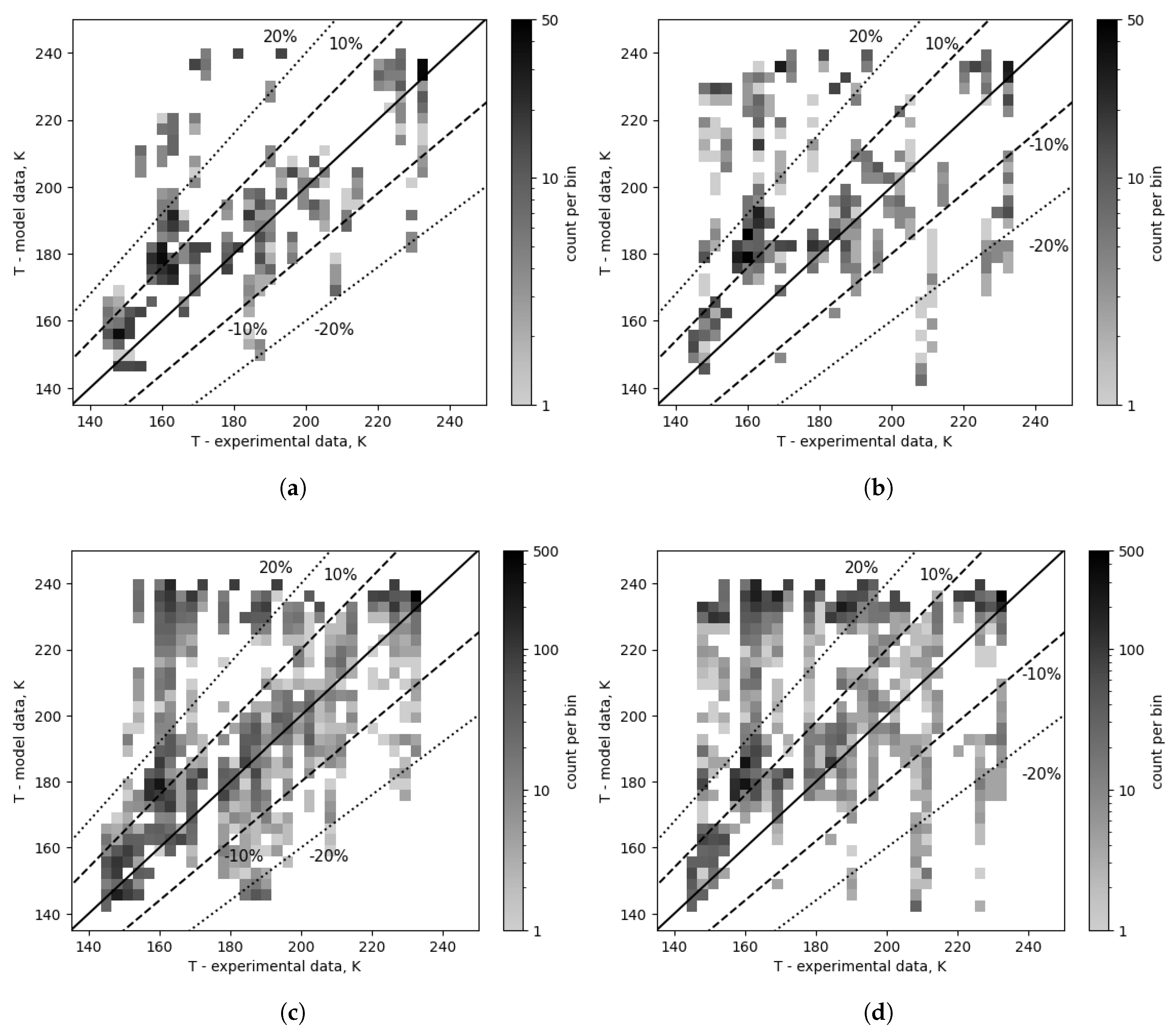
Figure 11.
Outlet temperature comparison for a selected evaporation combination (number 1: Hsieh & Lin) - composition corrected vs as measured. (a) Composition corrected cases - top 10. (b) Cases with composition as measured - top 10. (c) Composition corrected cases - top 96. (d) Cases with composition as measured - top 96.
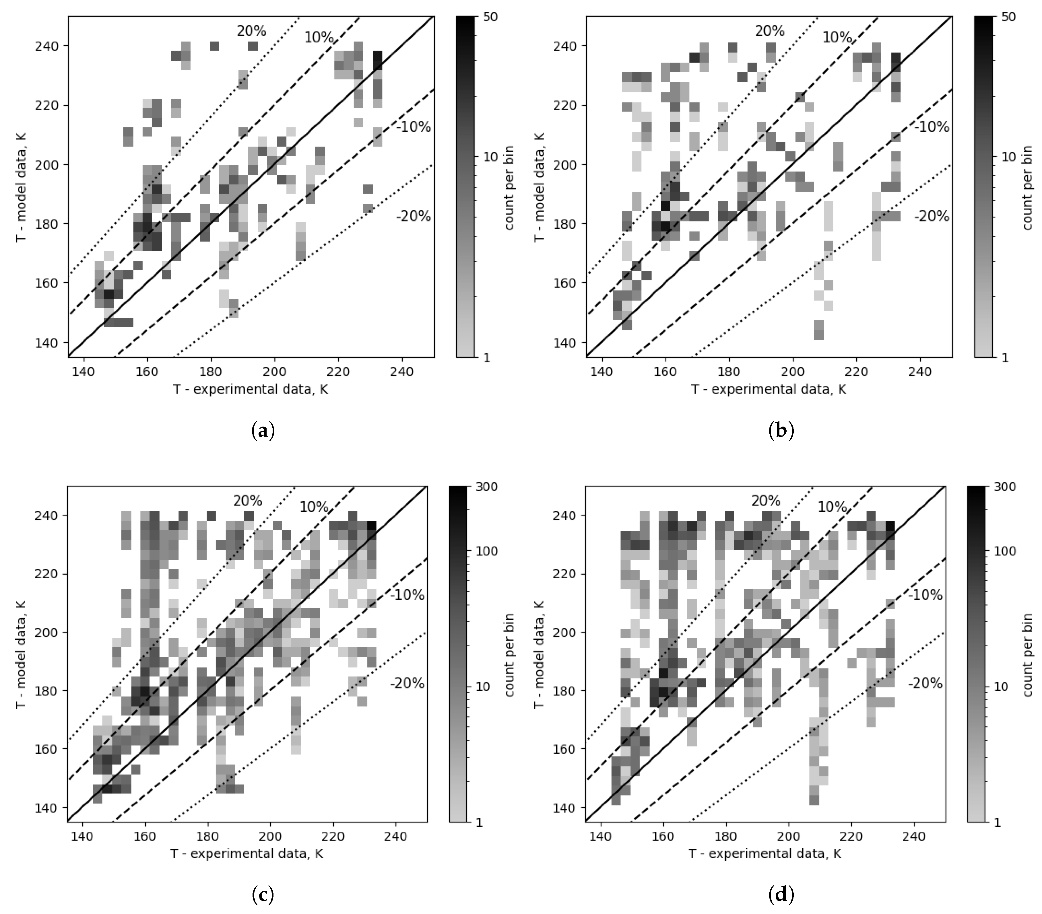
Figure 12.
Outlet temperature comparison for selected condensation correlations, Kuo and Thonon. (a) Condensation: Kuo (number 2), top 5. (b) Condensation: Thonon (number 1), top 5. (c) Condensation: Kuo (number 2), overall (top 24). (d) Condensation: Thonon (number 1), overall (top 24).
Figure 12.
Outlet temperature comparison for selected condensation correlations, Kuo and Thonon. (a) Condensation: Kuo (number 2), top 5. (b) Condensation: Thonon (number 1), top 5. (c) Condensation: Kuo (number 2), overall (top 24). (d) Condensation: Thonon (number 1), overall (top 24).
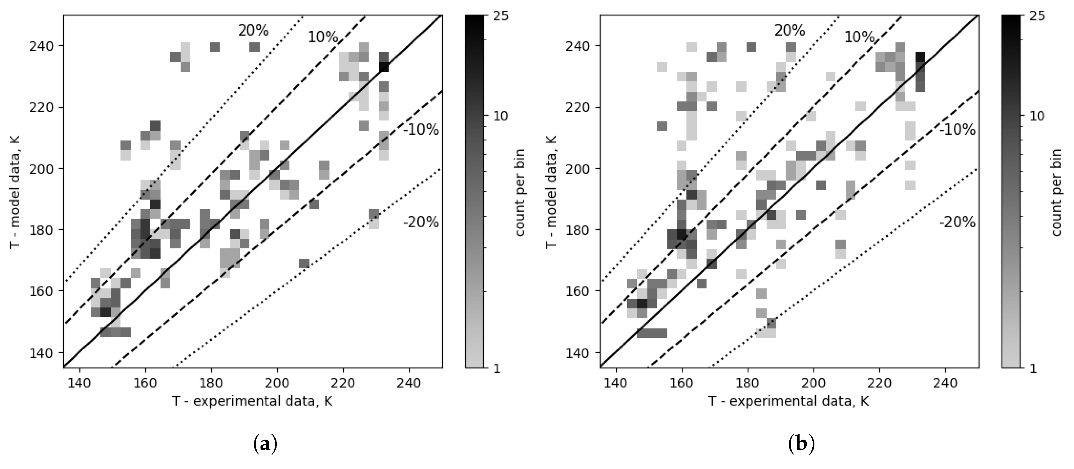
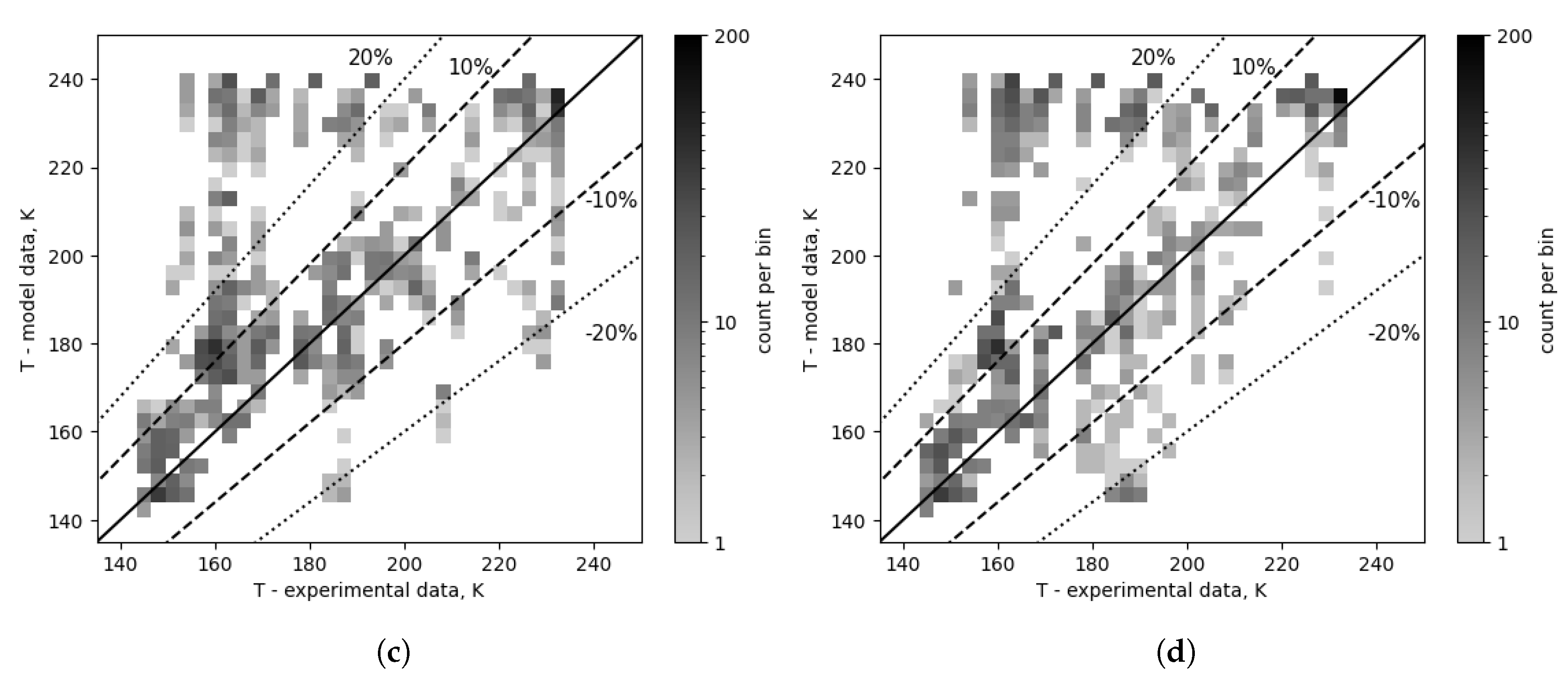
Figure 13.
Outlet temperature comparison for selected evaporation correlations. (a) Evaporation: Hsieh & Lin (number 1), top 5. (b) Evaporation: Han (number 0), top 5. (c) Evaporation: Hsieh & Lin (number 1), overall (top 48). (d) Evaporation: Han (number 0), overall (top 48).
Figure 13.
Outlet temperature comparison for selected evaporation correlations. (a) Evaporation: Hsieh & Lin (number 1), top 5. (b) Evaporation: Han (number 0), top 5. (c) Evaporation: Hsieh & Lin (number 1), overall (top 48). (d) Evaporation: Han (number 0), overall (top 48).
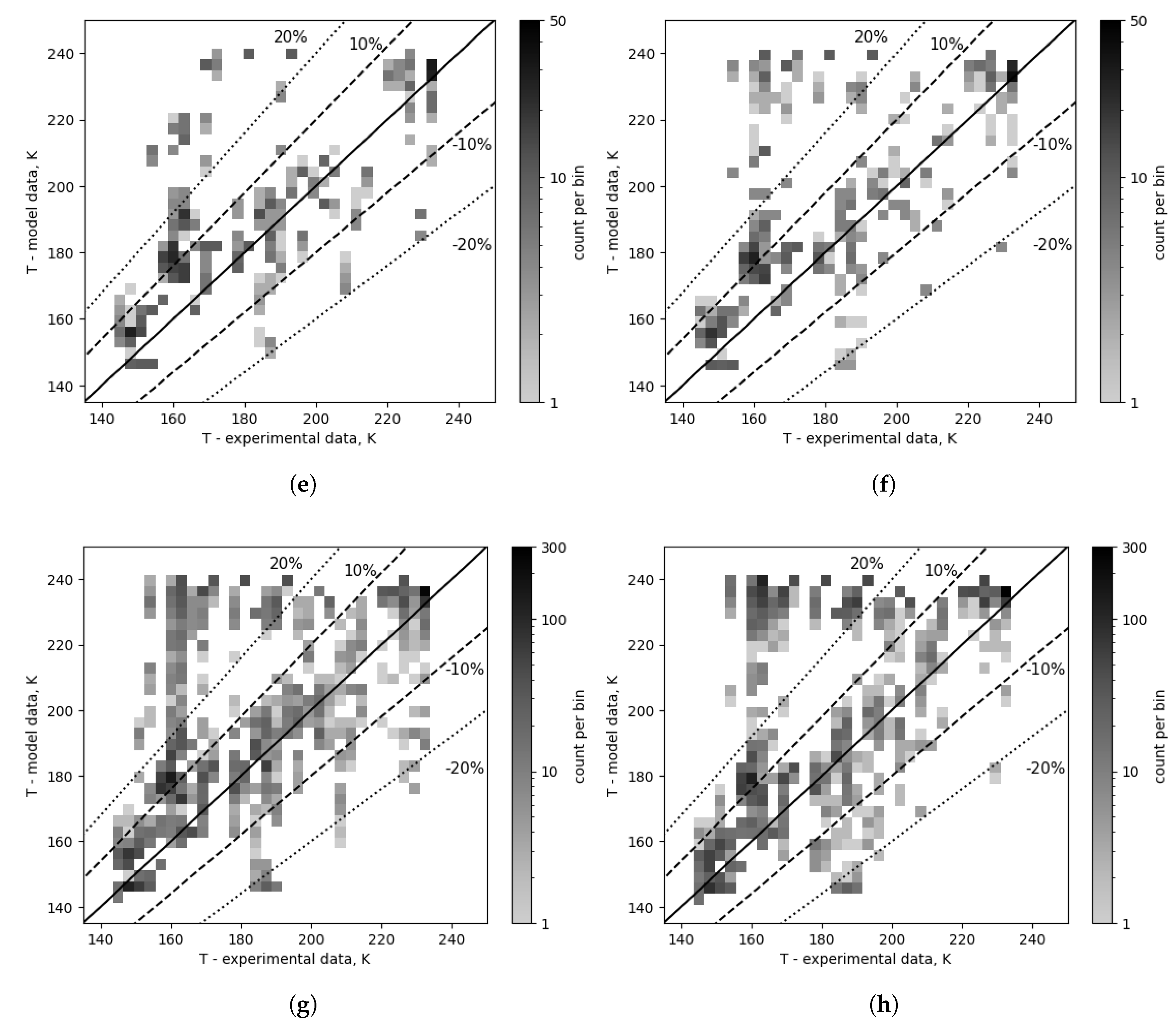
Figure 14.
Outlet temperature comparison of corrected and uncorrected evaporation. (a) Evaporation correction: Fujita (number 2), top 5. (b) Evaporation correction: none (number 0), top 5. (c) Evaporation correction: Fujita (number 2), overall (top 32). (d) Evaporation correction: none (number 0), overall (top 32).
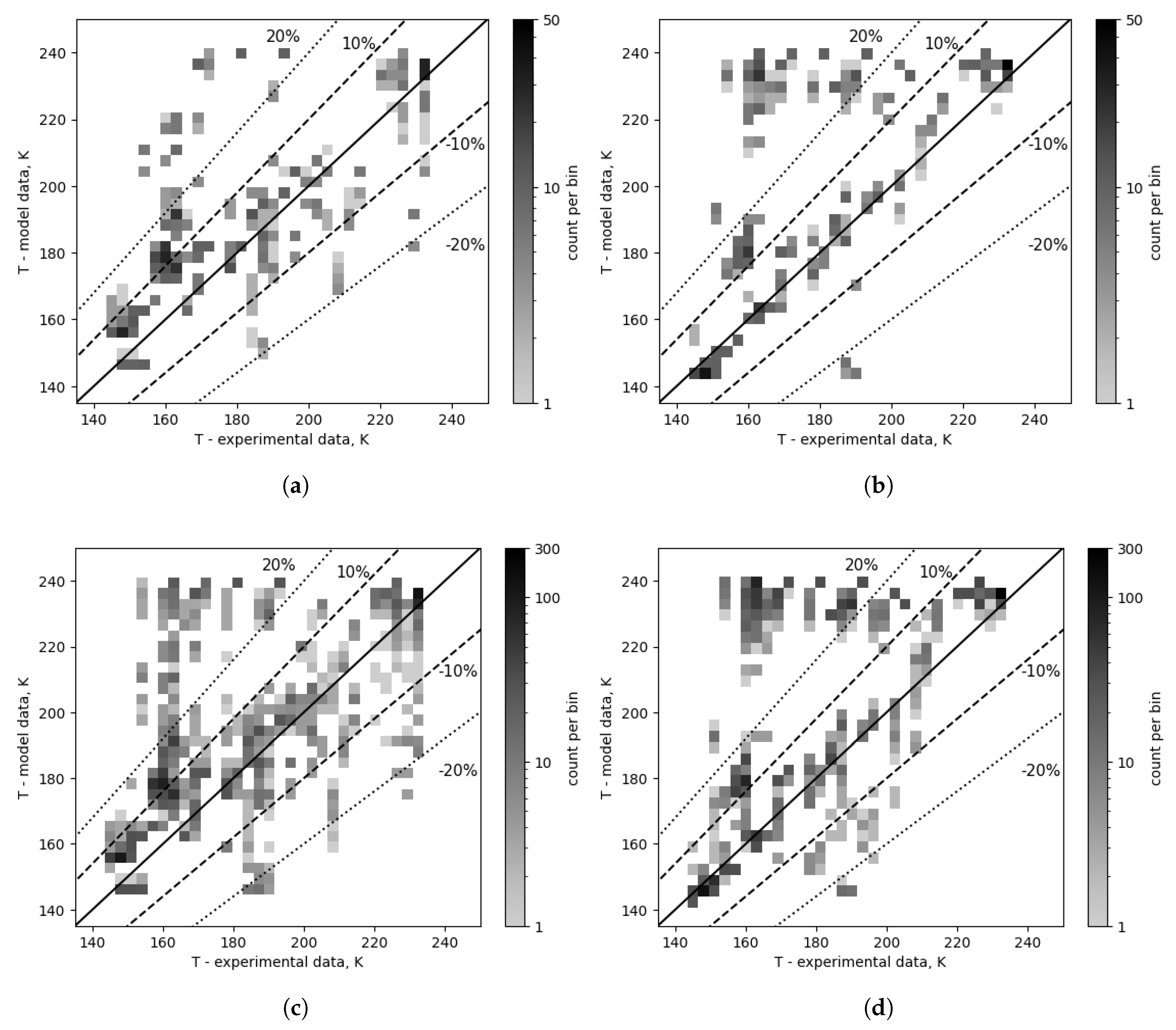
Figure 15.
Outlet temperature comparison - correlation combinations with the lowest and highest error, respectively. (a) Lowest MAE (top 1). (b) Highest MAE (top 96).
Figure 15.
Outlet temperature comparison - correlation combinations with the lowest and highest error, respectively. (a) Lowest MAE (top 1). (b) Highest MAE (top 96).
5.1. Statistical Analysis
Beside graphical interpretation of the results, statistical analysis has been applied to quantify the validation of the model and possibly capture some unclear trends and impacts. Differences among heat-transfer correlations were evaluated (, , , , ) and their combinations using a blocked, repeated-measures design at the level of a case (one experiment with fixed conditions). For each case and each correlation combination, the model reproduced outlet temperatures and point-wise errors and then case-level mean absolute error (MAE; Eq. 9) and root-mean-square error (RMSE; Eq. 10) were computed.
Because the composition of the mixture was found to significantly affect the thermal profile, the analyzes were performed in two modes: (i) the measured composition (AM; = 0) and (ii) the corrected composition (CC; = best), where for each (case times combination) the composition shift was selected minimizing the MAE for summary analyzes. Unless stated otherwise, all inferences are blocked by case.
For each heat transfer mechanism, marginal effects (case-wise averaging over other factors) were computed and ranked all 96 combinations by case-average MAE (and RMSE) (Table 6, Table 7, Table 8, Table 9, Table 10 and Table 11). Global differences among levels were tested with the Friedman test, and two-level contrasts with the Wilcoxon signed-rank test; pairwise post-hoc comparisons used Wilcoxon tests with Holm correction for multiplicity. Along with p-values we report effect sizes (median differences with 95% bootstrap CIs) and, where applicable, Cohen’s and Kendall’s W.
All analyzes were performed in Python (v3.8.8) using NumPy, pandas (v1.2.4), and SciPy (v1.6.2) for data handling and statistical testing. The bootstrap confidence intervals used the NumPy random generator with a fixed seed (42) for reproducibility.
5.2. Ranking and Marginal Effects
The Kuo et al. condensation correlation ranked first in both modes and differed significantly from the alternatives (Friedman, ; post-hoc Holm-adjusted Wilcoxon, ). For evaporation, Hsieh & Lin outperformed Han (AM: K; CC: K; both ). Among evaporation-correction correlations, Fujita et al. achieved the lowest marginal . Notably, with Sun et al. the inclusion of the boiling-heat-transfer correction yielded higher errors than without correction (all pairwise ). For single-phase heat transfer (hot/cold streams analyzed separately), Wanniarachchi consistently performed best, irrespective of stream or mode. The best overall combination (AM) achieved K, lower than the best single-factor marginal MAE (e.g., K), indicating that no single mechanism dominates and that joint selection of levels across mechanisms provides synergistic gains.
5.3. Effect of Composition Correction
Across all case × combination pairs, composition-corrected mode (CC) reduced errors relative to AM (Wilcoxon in =CC-AM): median K (95% CI), mean K, ; improvement occurred in 90.5% of comparisons. The optimal composition shift had median pp (Wilcoxon vs 0: ), suggesting a systematic positive bias in the measured composition.
Despite the reductions in absolute error, the rankings were largely preserved between modes (Kendall’s , ); 10/15 top combinations overlapped. Thus, composition uncertainty did not alter the choice of best-performing correlations in this dataset. CC estimates is regarded as an upper bound on achievable accuracy, since composition correction was tuned on the same data.
6. Conclusions
The paper concerns experimental and modeling analysis of recuperation heat transfer of methane-ethane binary mixtures in a precooled MR JT cryocooler with 3 BPHE connected in series as recuperators. The experimental campaign included measurement of the MR composition which was later implemented in the modeling. In addition, statistical analysis was used to fully postprocess the available data and some possible track trends and impacts in the data. In summary, following conclusions were drawn:
- 1.
- The combination of correlations with the lowest overall error was Kuo for condensation, Hsieh and Lin for evaporation with Fujita correction factor, and Wanniarachchi for single phase heat transfer. This combination was the best both for corrected and uncorrected composition modes.
- 2.
- Evaporation seems to be a dominating heat transfer factor which mostly governs overall heat transfer process. This can result from significant temperature differences between HP and LP streams during recuperation and potential of evaporation in film boiling regime. This topic requires further investigation.
- 3.
- The composition correction reduced the average MAE by 10.93 K (median -2.12 K), what emphasizes the importance of precise MR composition measurement, along with taking into account its uncertainty.
- 4.
- The optimal MR composition shift has median pp suggesting that there is a systematic positive bias in the measured composition.
- 5.
- MR with more components are less sensitive to the accuracy of MR composition measurement. In case of binary high-temperature glide MR even small uncertainty can lead to significant change of recuperation temperature profile.
- 6.
- Taking into account the complexity of recuperation heat transfer for MR (which depends on number and type of components, MR composition measurement accuracy and combines several heat transfer mechanisms and for gaseous, liquid and 2-phase flows) it requires further investigations.
Acknowledgments
This research was partially supported by the Ministry of Science and Higher Education, grant number: DWD/6/0541/2022. This research was partially supported by the statutory funds of the Faculty of Mechanical and Power Engineering, Wrocław University of Science and Technology.
Conflicts of Interest
The authors declare no conflicts of interest.
Abbreviations
The following abbreviations are used in this manuscript:
| AM | As-measured composition mode |
| AC | Air cooler |
| BPHE | Brazed plate heat exchanger |
| BT | Buffer tank |
| C | Compressor |
| CD | Condensation heat transfer correlation |
| CFM | Coriolis flow meter |
| CC | Composition corrected mode |
| CF | Correction factor |
| CV | Control valve |
| DP | Differential pressure transducer |
| EH | Electric heater |
| EV | Evaporation heat transfer correlation |
| Evaporation heat transfer correlation with correction factor | |
| F | Flow meter |
| FL | Filter drier |
| GM | Gifford-McMahon |
| HC | hydrocarbon |
| HEB | High error band |
| HP | High pressure |
| HTC | Heat transfer coefficient |
| HX | Heat exchanger |
| JT | Joule-Thomson |
| LMTD | Logarithmic mean temperature difference |
| LP | Low pressure |
| MAE | Mean absolute error |
| MCHE | Microchannel heat exchanger |
| MR | Mixed-refrigerant |
| MV | Manual valve |
| N | Power meter |
| NC | Not corrected |
| Nu | Nusselt number |
| NTU | Number of heat transfer Units |
| OR | Oil removal |
| P | Pump |
| P&ID | Piping and Instrumentation Design |
| Pr | Prandtl number |
| RMSE | Root-mean-square error |
| SeV | Service valve |
| SG | Sight glass |
| SP | Single phase |
| SV | Solenoid valve |
| Single-phase heat transfer correlation for cooling | |
| Single-phase heat transfer correlation for heating | |
| XPS | Extruded polystyrene |
| physical quantity | |
| heat capacity rate | |
| NTU | number of thermal units |
| numerical error | |
| numerical error tolerance | |
| effectiveness of the heat exchanger | |
| heat transfer rate |
References
- Rogala, Z.; Siemasz, R.; Baran, B.; Kwiatkowski, A. Design and experimental study on precooled MR JT cryocooler for LNG recondensation purposes. Applied Thermal Enginnering 2022. [Google Scholar] [CrossRef]
- Pang, W.; Liu, J.; Xu, X. A strategy to optimize the charge amount of the mixed refrigerant for the Joule – Thomson cooler. International Journal of Refrigeration 2016, 69, 466–479. [Google Scholar] [CrossRef]
- Bychkov, E.G. An analytical method for ensuring the optimal circulating composition of the multicomponent refrigerant mixture in a steady-state operation mode of the Joule-Thomson refrigerator operating with mixtures. International Journal of Refrigeration 2021, 130, 356–369. [Google Scholar] [CrossRef]
- Rogala, Z. Application of precooling stage in MR JT cryocoolers. Cryogenics 2022, 121, 103395. [Google Scholar] [CrossRef]
- Kwiatkowski, A.; Rogala, Z.; Poliński, J.; Siemasz, R.; Wnukowski, M. Noninvasive and continuous method of binary and ternary mixture composition measurement. International Journal of Refrigeration 2026. [Google Scholar] [CrossRef]
- Damle, R.; Ardhapurkar, P.; Atrey, M. Numerical analysis of the two-phase heat transfer in the heat exchanger of a mixed refrigerant Joule–Thomson cryocooler. Cryogenics 2015. [Google Scholar] [CrossRef]
- Baek, S.; Lee, C.; Jeong, S. Investigation of two-phase heat transfer coefficients of argon–freon cryogenic mixed refrigerants. Cryogenics 2014. [Google Scholar] [CrossRef]
- Nellis, G.; Hughes, C.; Pfotenhauer, J. Heat transfer coefficient measurements for mixed gas working fluids at cryogenic temperatures. Cryogenics 2005, 45, 546–556. [Google Scholar] [CrossRef]
- Gong, M.Q. Research on the change of mixture compositions in mixed-refrigerant Joule-Thomson cryocoolers. 2002, 881, 881–886. [Google Scholar] [CrossRef]
- Ardhapurkar, P.M.; Sridharan, A.; Atrey, M.D. Investigations on two-phase heat exchanger for mixed refrigerant JouleThomson cryocooler. Proceedings of the AIP Conference Proceedings 2012, Vol. 1434, 706–713. [Google Scholar] [CrossRef]
- Ardhapurkar, P.M.; Sridharan, A.; Atrey, M.D. Experimental investigation on temperature profile and pressure drop in two-phase heat exchanger for mixed refrigerant Joule-Thomson cryocooler. Applied Thermal Engineering 2014, 66, 94–103. [Google Scholar] [CrossRef]
- Gong, M.; Zhou, W.; Wu, J. Composition Shift due to the Different Solubility in the Lubricant Oil for Multicomponent Mixtures. Proceedings of the Cryocoolers 14 2007, Vol. 14, 459–467. [Google Scholar]
- Gong, M.; Deng, Z.; Wu, J. Composition Shift of a Mixed-Gas Joule-Thomson Refrigerator Driven by an Oil-Free Compressor. Proceedings of the Cryocoolers 2007, 14, 453–458. [Google Scholar]
- Lakshmi Narasimhan, N.; Venkatarathnam, G. A method for estimating the composition of the mixture to be charged to get the desired composition in circulation in a single stage JT refrigerator operating with mixtures. Cryogenics 2010, 50, 93–101. [Google Scholar] [CrossRef]
- N.Lakshmi Narasimhan, G. Effect of mixture composition and hardware on the performance of a single stage JT refrigerator. Cryogenics 2011, 51, 446–451. [CrossRef]
- Lemmon, E.W.; Bell, I.H.; Huber, M.L.; McLinden, M.O. NIST Standard Reference Database 23: Reference Fluid Thermodynamic and Transport Properties-REFPROP, Version 10.0; National Institute of Standards and Technology, 2018. [Google Scholar] [CrossRef]
- Wanniarachchi, A.S.; Ratnam, U.V.; Tilton, B.E.; Dutta-Roy, K. Approximate correlations for chevron-type plate heat exchangers; 1995. [Google Scholar]
- Yan, Y.Y.; Lio, H.C.; Lin, T.F. Condensation heat transfer and pressure drop of refrigerant R-134a in a plate heat exchanger. International Journal of Heat and Mass Transfer 1999, 42, 993–1006. [Google Scholar] [CrossRef]
- Han, D.H.; Lee, K.J.; Kim, Y.H. Experiments on the characteristics of evaporation of R410A in brazed plate heat exchangers with different geometric configurations. Applied Thermal Engineering 2003, 23, 1209–1225. [Google Scholar] [CrossRef]
- Khan, T.; Khan, M.; Chyu, M.C.; Ayub, Z. Experimental investigation of single phase convective heat transfer coefficient in a corrugated plate heat exchanger for multiple plate configurations. Applied Thermal Engineering 2010, 30, 1058–1065. [Google Scholar] [CrossRef]
- Thonon, B.; Bontemps, A. Condensation of Pure and Mixture of Hydrocarbons in a Compact Heat Exchanger: Experiments and Modelling. Heat Transfer Engineering 2002, 23, 3–17. [Google Scholar] [CrossRef]
- Hsieh, Y.; Lin, T. Saturated flow boiling heat transfer and pressure drop of refrigerant R-410A in a vertical plate heat exchanger. International Journal of Heat and Mass Transfer 2002, 45, 1033–1044. [Google Scholar] [CrossRef]
- Sun, Z.; Gong, M.; Li, Z.; Wu, J. Nucleate pool boiling heat transfer coefficients of pure HFC134a, HC290, HC600a and their binary and ternary mixtures. International Journal of Heat and Mass Transfer 2007, 50, 94–104. [Google Scholar] [CrossRef]
- Kuo, W.; Lie, Y.; Hsieh, Y.; Lin, T. Condensation heat transfer and pressure drop of refrigerant R-410A flow in a vertical plate heat exchanger. International Journal of Heat and Mass Transfer 2005, 48, 5205–5220. [Google Scholar] [CrossRef]
- Fujita, Y.; Tsutsui, M. Heat transfer in nucleate pool boiling of binary mixtures. International Journal of Heat and Mass Transfer 1994, 37, 291–302. [Google Scholar] [CrossRef]
- Han, D.H.; Lee, K.J.; Kim, Y.H. The Characteristics of Condensation in Brazed Plate Heat Exchangers with Different Chevron Angles. Journal- Korean Physical Society 2003, 43, 66–73. [Google Scholar]
Figure 1.
P&ID of the test stand
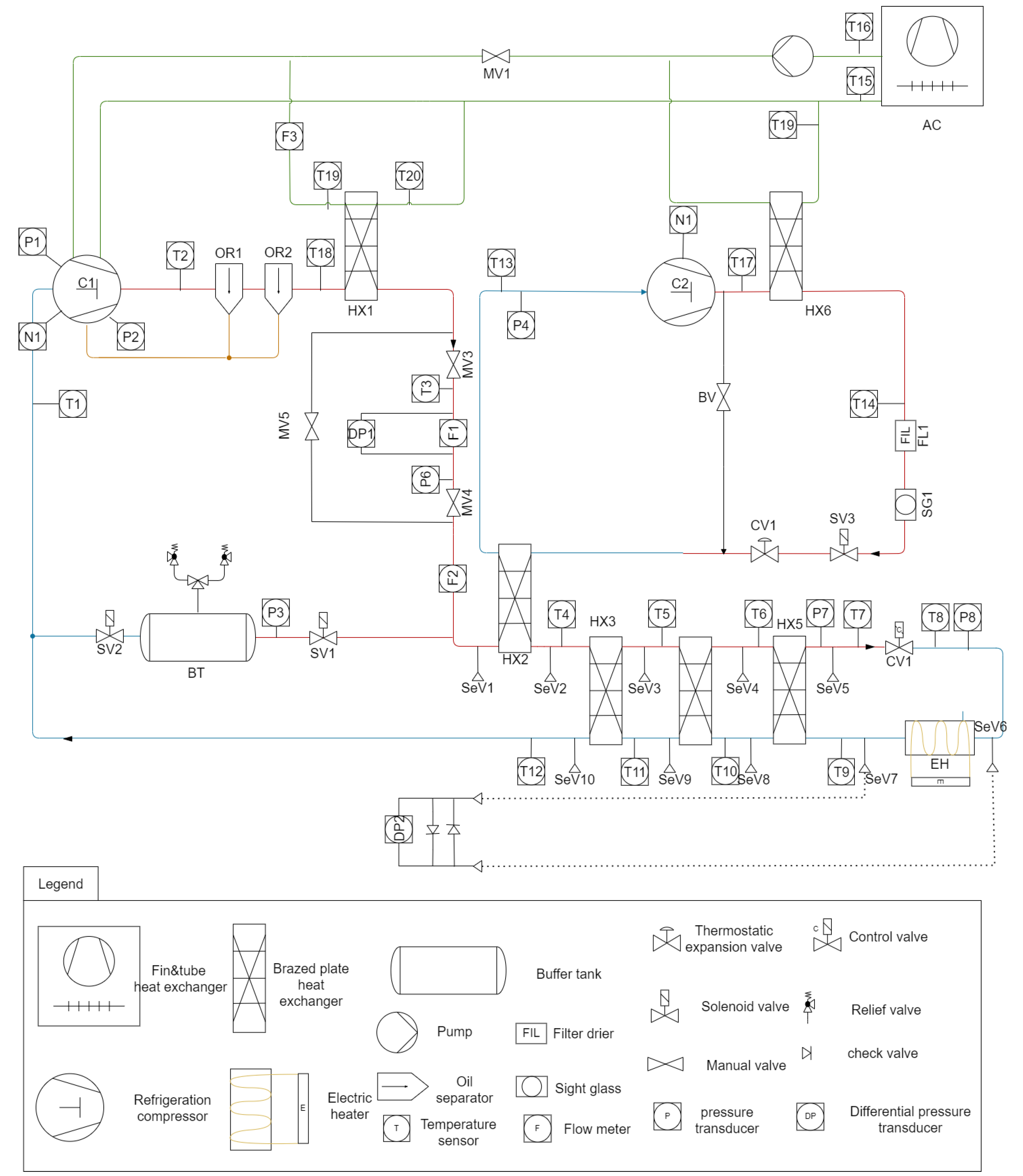
Figure 2.
Layout of the coldbox
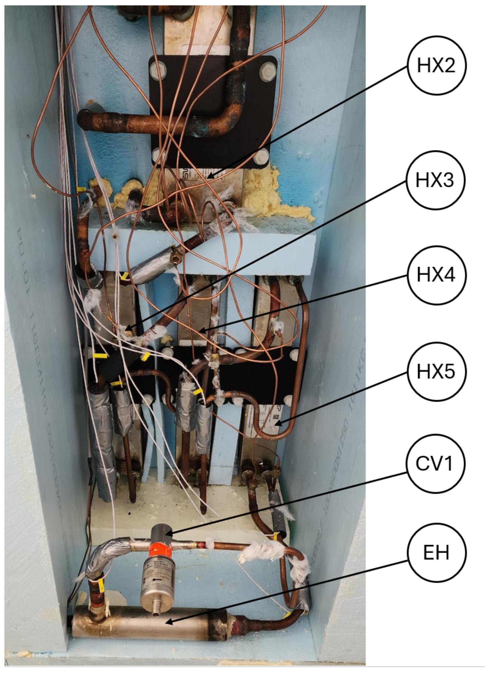
Figure 3.
Cooldown and stabilization of the system.
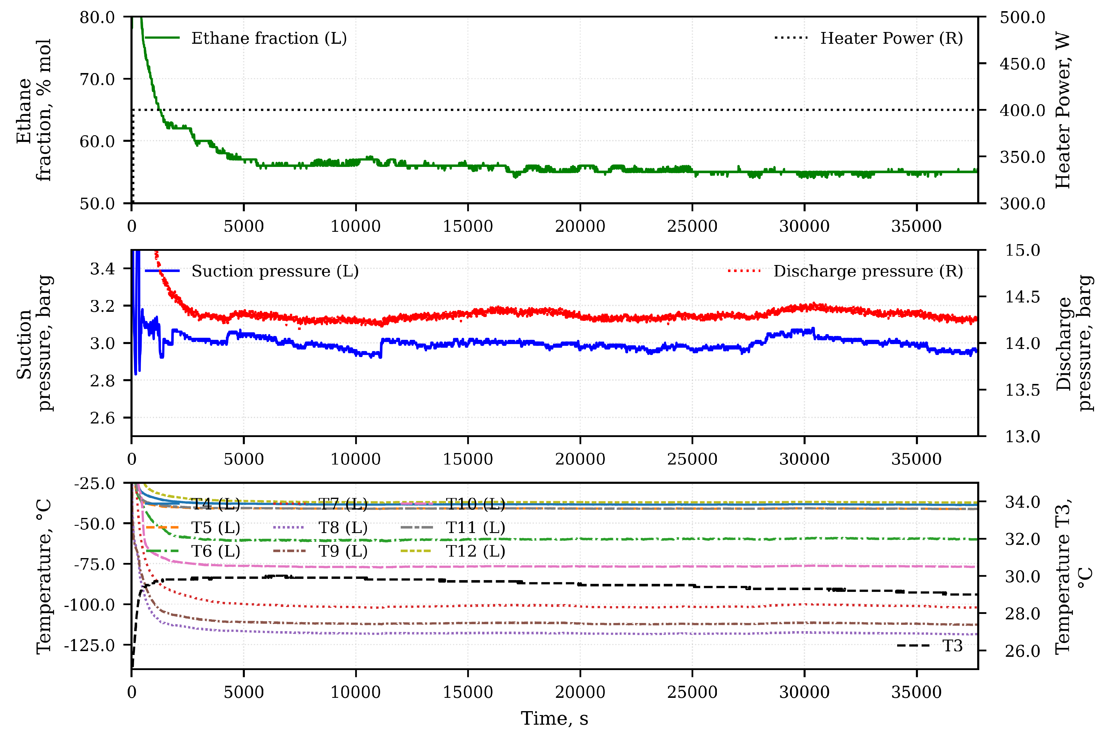
Figure 5.
Numerical model scheme.
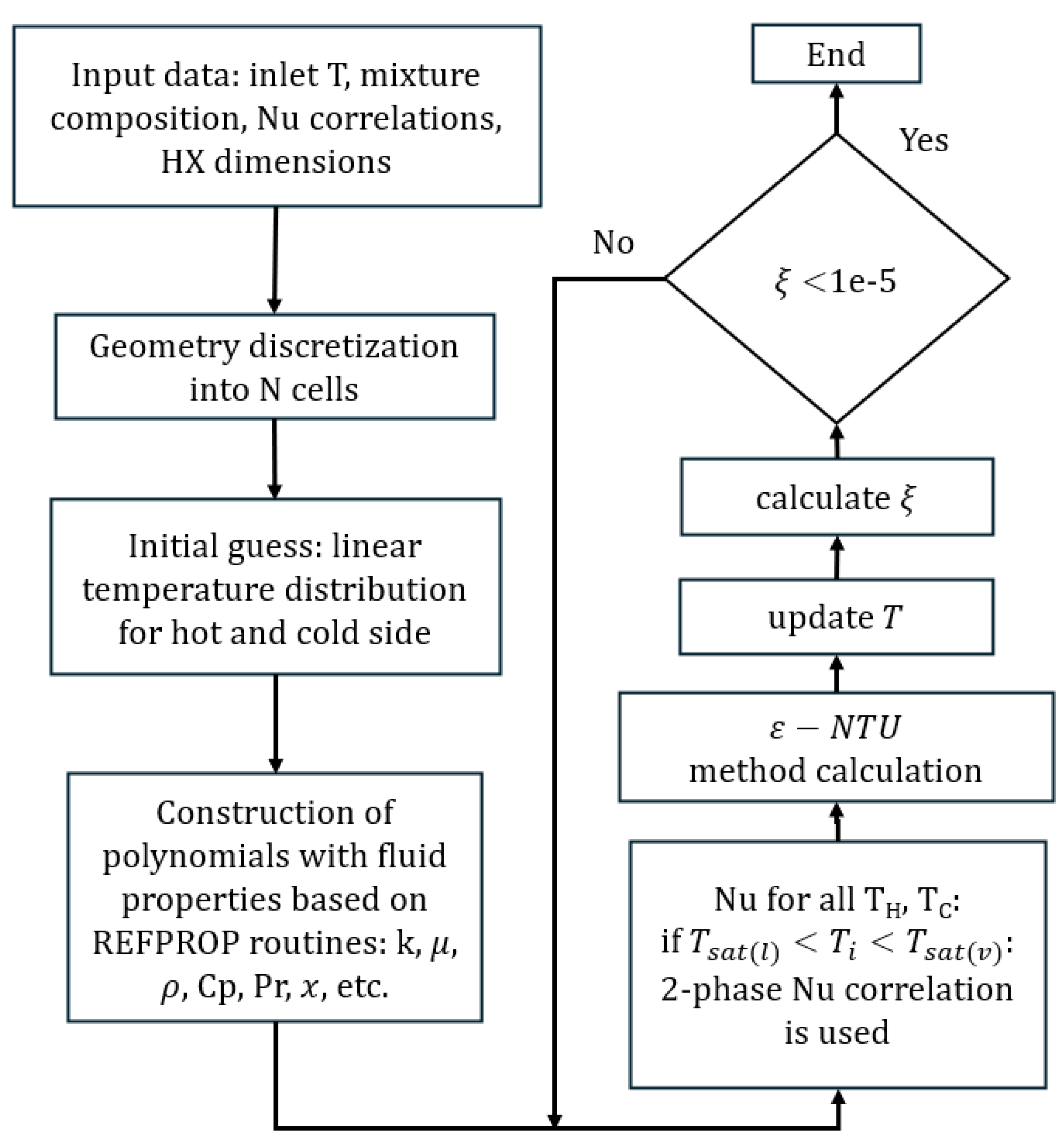

Table 1.
Specification of the applied instrumentation.
| Measured property | Description | Uncertainty | Remarks |
| Temperature | Pt100, class B, 3-wire | ± (0.3+0.005t) °C | -196 to 150 °C |
| Pressure | Peltron NPX | ± 0.1% FS | P6 (0 to 20 barg) |
| Pressure | Johnson Controls P499 | ± 0.25% FS | P7 (0 to 30 barg) |
| Pressure | Johnson Controls P499 | ± 0.25% FS | P8 (-1 to 8 barg) |
| Pressure | Carel SPKT | ± 1% FS | P1-P5 (0 to 30 barg) |
| MR mass flow | CFM E+H Promass 83F | ± 0.5 % of reading | |
| MR density | CFM E+H Promass 83F | ±0.37 | validated by [5] |
Table 2.
Design of experiment.
| Methane [%] | Ethane [%] | HP [bar] | LP [bar] | [Hz] |
| 40 | 60 | 15 | 3 | 50 |
| 40 | 60 | 15 | 3 | 50 |
| 40 | 60 | 15 | 2 | 30 |
| 40 | 60 | 20 | 3 | 30 |
| 40 | 60 | 20 | 2 | 50 |
| 40 | 60 | 15 | 2 | 30 |
| 40 | 60 | 20 | 3 | 30 |
| 40 | 60 | 20 | 2 | 50 |
| 50 | 50 | 20 | 3 | 30 |
| 50 | 50 | 20 | 3 | 30 |
| 50 | 50 | 15 | 2 | 30 |
| 50 | 50 | 15 | 2 | 30 |
| 50 | 50 | 15 | 3 | 50 |
| 50 | 50 | 20 | 2 | 50 |
| 50 | 50 | 15 | 3 | 50 |
| 50 | 50 | 20 | 2 | 50 |
Table 3.
Correlations and correction factors used. SP - single phase, CD - condensation, EV - evaporation - evaporation correction.
Table 3.
Correlations and correction factors used. SP - single phase, CD - condensation, EV - evaporation - evaporation correction.
| Number | Single phase | Condensation | Evaporation | Evaporation |
| correction | ||||
| 0 | Wanniarachchi [17] | Yan [18] | Han [19] | None |
| 1 | Khan [20] | Thonon [21] | Hsieh & Lin [22] | Sun [23] |
| 2 | - | Kuo [24] | - | Fujita [25] |
| 3 | - | Han [26] | - | - |
Table 4.
Distribution of data points - composition correction. HEB - high error band. AM - composition as measured. CC - composition corrected results.
Table 4.
Distribution of data points - composition correction. HEB - high error band. AM - composition as measured. CC - composition corrected results.
| Range | Overall, AM (CC) | Top 15, AM (CC) | Hsieh & Lin AM, (CC) |
| ±30% | 73.9 (84.4) | 84.6 (92.5) | 76.7 (87.3) |
| ±20% | 59.3 (75.9) | 73.3 (88.4) | 62.5 (79.2) |
| ±10% | 36.3 (58.9) | 45.5 (66.6) | 37.7 (60.8) |
| HEB | 29.7 (15.1) | 13.6 (2.7) | 26.3 (11.6) |
Table 5.
Distribution of data points-comparison of correlations. HEB - high error band. CD - condensation. EV - evaporation. NC - not corrected evaporation. CF - evaporation correction factor used.
Table 5.
Distribution of data points-comparison of correlations. HEB - high error band. CD - condensation. EV - evaporation. NC - not corrected evaporation. CF - evaporation correction factor used.
| Range | Kuo (CD) | Thonon (CD) | Han (EV) | Hsieh & Lin (EV) | EV (NC) | EV (CF) |
| ±30% | 88.9 | 82.7 | 84.6 | 92.5 | 76.7 | 87.3 |
| ±20% | 82.1 | 73.5 | 73.3 | 88.4 | 62.5 | 79.2 |
| ±10% | 62.4 | 56.8 | 45.5 | 66.6 | 37.7 | 60.8 |
| HEB | 26.3 | 11.6 | 13.6 | 2.7 | 26.3 | 11.6 |
Table 6.
Best combinations of equations.
| EV | CD | MAE (corrected) | RMSE (corrected) | MAE | RMSE | Rank (corrected) | Rank | |||
| 1 | 1 | 2 | 0 | 0 | 16.15 | 18.15 | 24.00 | 26.98 | 1 | 1 |
| 1 | 1 | 2 | 0 | 1 | 16.22 | 18.28 | 24.43 | 27.38 | 2 | 7 |
| 1 | 1 | 2 | 1 | 1 | 16.23 | 18.34 | 24.70 | 27.66 | 3 | 8 |
| 1 | 1 | 2 | 1 | 0 | 16.24 | 18.23 | 24.18 | 27.21 | 4 | 2 |
| 0 | 2 | 2 | 0 | 0 | 16.39 | 18.45 | 25.74 | 28.66 | 5 | 10 |
| 0 | 2 | 2 | 1 | 0 | 16.53 | 18.48 | 25.94 | 28.83 | 6 | 12 |
| 0 | 2 | 2 | 0 | 1 | 16.54 | 18.53 | 26.20 | 29.17 | 7 | 15 |
| 0 | 2 | 2 | 1 | 1 | 16.65 | 18.63 | 26.52 | 29.44 | 8 | 18 |
| 1 | 2 | 3 | 0 | 0 | 16.70 | 18.93 | 25.31 | 28.04 | 9 | 9 |
| 1 | 2 | 3 | 1 | 0 | 16.72 | 18.96 | 25.77 | 28.50 | 10 | 11 |
| 1 | 2 | 3 | 1 | 1 | 16.73 | 19.11 | 26.64 | 29.49 | 11 | 20 |
| 1 | 2 | 3 | 0 | 1 | 16.87 | 19.35 | 26.52 | 29.34 | 12 | 19 |
| 1 | 2 | 0 | 0 | 0 | 16.88 | 19.15 | 25.94 | 28.69 | 13 | 13 |
| 1 | 2 | 0 | 1 | 0 | 16.91 | 19.22 | 26.42 | 29.17 | 14 | 16 |
| 1 | 2 | 0 | 0 | 1 | 16.95 | 19.36 | 27.11 | 30.07 | 15 | 21 |
Table 7.
Comparison of condensation equations - MAE&RMSE.
| CD | MAE (corrected) | RMSE (corrected) | MAE | RMSE |
| 2 | 19.41 | 22.16 | 29.14 | 32.60 |
| 3 | 22.90 | 25.96 | 34.22 | 37.88 |
| 0 | 23.10 | 26.27 | 34.50 | 38.23 |
| 1 | 23.32 | 26.38 | 34.59 | 38.25 |
Table 8.
Comparison of evaporation equations - MAE&RMSE.
| EV | MAE (corrected) | RMSE (corrected) | MAE | RMSE |
| 1 | 20.23 | 22.89 | 31.24 | 34.65 |
| 0 | 24.14 | 27.49 | 34.99 | 38.83 |
Table 9.
Comparison of evaporation correction equations - MAE&RMSE.
| MAE (corrected) | RMSE (corrected) | MAE | RMSE | |
| 2 | 19.04 | 21.50 | 28.71 | 31.80 |
| 1 | 21.84 | 24.66 | 32.85 | 36.30 |
| 0 | 25.68 | 29.41 | 37.77 | 42.12 |
Table 10.
Comparison of single phase equations on cold stream - MAE&RMSE.
| MAE (corrected) | RMSE (corrected) | MAE | RMSE | |
| 0 | 21.83 | 24.74 | 32.59 | 36.13 |
| 1 | 22.54 | 25.64 | 33.63 | 37.35 |
Table 11.
Comparison of single phase equations on hot stream - MAE&RMSE.
| MAE (corrected) | RMSE (corrected) | MAE | RMSE | |
| 0 | 21.99 | 24.95 | 32.85 | 36.44 |
| 1 | 22.38 | 25.44 | 33.38 | 37.04 |
Disclaimer/Publisher’s Note: The statements, opinions and data contained in all publications are solely those of the individual author(s) and contributor(s) and not of MDPI and/or the editor(s). MDPI and/or the editor(s) disclaim responsibility for any injury to people or property resulting from any ideas, methods, instructions or products referred to in the content. |
© 2026 by the authors. Licensee MDPI, Basel, Switzerland. This article is an open access article distributed under the terms and conditions of the Creative Commons Attribution (CC BY) license (http://creativecommons.org/licenses/by/4.0/).
Copyright: This open access article is published under a Creative Commons CC BY 4.0 license, which permit the free download, distribution, and reuse, provided that the author and preprint are cited in any reuse.


