
Submitted:
24 January 2026
Posted:
26 January 2026
You are already at the latest version
Abstract
This study investigates the performance of four deep learning architectures including Long Short-Term Memory (LSTM), Gated Recurrent Unit (GRU), Convolutional Neural Network (CNN) and Transformer for univariate time-series forecasting. To evaluate their ability in capturing different temporal dynamics, we selected two contrasting datasets: Apple Inc.\ (AAPL) stock prices, characterized by noise and volatility without clear seasonality and Melbourne’s daily minimum temperatures, which exhibit strong seasonal patterns. Each model was trained using consistent configurations and evaluated using standard metrics. Our results show that GRU and LSTM perform best across both domains, particularly in handling abrupt changes in financial data, while CNN and Transformer show competitive performance on smoother seasonal data. The findings highlight the importance of aligning model architecture with the underlying structure of the time series.
Keywords:
univariate time-series forecasting
; Long Short-Term Memory
; Gated Recurrent Unit
; Convolutional Neural Network and Transformer Network
1. Introduction
Time-series forecasting is a fundamental task in machine learning with critical applications across finance, energy management, weather prediction, and healthcare [1]. Traditional statistical models such as ARIMA, Exponential Smoothing, and Kalman Filters have shown effectiveness for linear and stationary sequences, but they tend to struggle with nonlinear dynamics and long-range dependencies [2].
In recent years, deep learning techniques have demonstrated remarkable success in modeling complex time-series patterns [3]. Among these, Long Short-Term Memory (LSTM) first introduced by Hochreiter and Schmidhuber, effectively capture long-range patterns in sequential data [4]. Gated Recurrent Units (GRUs) offer a streamlined alternative to LSTMs, reducing computational demands while maintaining performance [5]. Convolutional Neural Networks (CNNs), although originally designed for images, have been successfully adapted for time-series forecasting, achieving competitive accuracy with improved efficiency [6,7]. More recently, Transformer architectures, driven by self-attention mechanisms, have shown excellent results in capturing both short and long term dependencies in time-series data [8,9,10]. These models allow for parallelization and often outperform recurrent structures in long-horizon forecasting tasks. Several recent reviews and benchmarking studies have shown that deep neural networks, especially Transformers are highly effective across various domains such as stock market prediction, energy load forecasting, and weather modeling [11,12].
Despite this success, each neural architecture has unique trade-offs in terms of accuracy, generalization and computational requirements. Thus, a comparative study of LSTM, GRU, CNN, and Transformer models can provide valuable insights for practitioners. This paper performs such a comparison on standardized univariate datasets and evaluates each model’s forecasting quality and training efficiency across multiple benchmarks.
2. Methodology
This study evaluates the performance of four deep leaning architectures: LSTM, GRU, CNN, and Transformer, on univariate time-series forecasting tasks. Each model is trained and tested using standardized datasets with appropriate normalization and windowing strategies to ensure fair comparisons. The models are implemented using PyTorch and trained on the same hardware environment to control for computational bias. The evaluation focuses on both forecasting accuracy and training efficiency under consistent settings. The methodology is divided into four parts: (i) description of datasets, (ii) preprocessing steps, (iii) details of model architectures and (iii) training configuration.
2.1. Dataset
To ensure diversity and robustness in our evaluation, we selected two distinct univariate time-series datasets: one financial and one environmental. These datasets were deliberately chosen to capture diverse temporal dynamics and test the adaptability of neural network models under different conditions. The stock price data from Apple Inc. (AAPL) represents a financial time-series that is typically noisy, non-stationary, and influenced by external market factors, offering a challenging benchmark for models to capture short-term fluctuations and trends. In contrast, the Melbourne minimum temperature dataset exhibits strong seasonal patterns and smoother temporal continuity, making it ideal for assessing how well models can learn and generalize periodic behaviors. By using these two contrasting datasets, we aim to evaluate the robustness and forecasting capabilities of LSTM, GRU, CNN, and Transformer architectures across both high-volatility and seasonally structured time-series data.
1) Financial Dataset: We used daily closing stock prices of Apple Inc. (AAPL) obtained from Yahoo Finance1 covering the period from January 2015 to December 2022. The dataset includes features such as Open, High, Low, Close and Volume, but only the Close price was used for forecasting. Missing values (e.g., weekends, holidays) were handled by forward-filling.
2) Environmental Dataset: We used the Daily Minimum Temperature dataset collected in Melbourne, Australia, available on Kaggle2. It contains daily minimum temperature records from 1981 to 1990 and is clean and free from missing values, making it ideal for benchmarking.
2.2. Preprocessing
Both datasets were normalized to the range using Min-Max scaling. Normalization to the range was applied to ensure numerical stability and to facilitate efficient training. Neural networks are sensitive to input scale, and Min-Max scaling helps standardize the data range, resulting in faster convergence and more balanced weight updates during optimization. A sliding window technique was used to convert the data into supervised learning format, where a window of n previous observations is used to predict the next time step. We used a window size of days for all models. The data was split into training (70%), validation (15%), and test (15%) sets.
2.3. Model Architectures
We implemented four deep learning models; LSTM, GRU, CNN and Transformer, each designed to handle univariate time-series forecasting tasks. Our LSTM and GRU architectures both employ two recurrent layers with 64 hidden units—a configuration shown to balance model capacity and convergence for sequential data [3,13]. The CNN model uses one-dimensional convolutional layers with kernel sizes of 3 and 5, inspired by empirical evidence that multiple small kernels effectively capture both local and broader temporal features in time-series [6,14]. For the Transformer, we use two encoder layers with four attention heads and a feed-forward dimension of 128; this setup was found in recent surveys to provide strong performance on long-horizon forecasting tasks without over-parameterization [3,15]. We also applied positional encodings to preserve sequence ordering, as standard in Transformer architectures. All models are trained on input sequences of length 30, derived using a sliding window method, which offers a good trade-off between capturing temporal context and computational efficiency [3]. This configuration ensures consistent input dimensions and fair comparison across models.
2.4. Training Configuration
All models were implemented using the PyTorch framework and trained under identical conditions to ensure fair performance comparison. Mean Squared Error (MSE) was used as the loss function, which is commonly applied in regression-based forecasting problems due to its sensitivity to large deviations. The Adam optimizer was used for all models with a learning rate of . Adam combines the benefits of AdaGrad and RMSProp and is known for its fast convergence in deep learning tasks. Each model was trained for 100 epochs with early stopping based on validation loss to prevent overfitting. A patience parameter of 10 was used for early stopping. The batch size was set to 64 across all models, balancing convergence speed and memory efficiency. The time-series data was split chronologically into training (70%), validation (15%), and test (15%) sets to avoid lookahead bias. The validation set was used for hyperparameter tuning and early stopping, while the test set was reserved strictly for final performance evaluation. All experiments were conducted on a laptop equipped with an 11th Gen Intel(R) Core(TM) i7-1165G7 CPU and 16 GB RAM, without GPU acceleration. Despite hardware limitations, all models including the Transformer were successfully trained using CPU-based execution.
3. Results and Analysis
This section presents a comparative analysis of the LSTM, GRU, CNN, and Transformer models based on their performance in forecasting two univariate time-series datasets: Apple (AAPL) stock prices and Melbourne minimum daily temperatures. We use both quantitative evaluation metrics and visual inspection of the predicted trends to understand each model’s strengths and weaknesses.
3.1. Quantitative Analysis
To evaluate model performance on both datasets, we used three standard regression metrics: Mean Absolute Error (MAE), Root Mean Square Error (RMSE), and Mean Absolute Percentage Error (MAPE). MAE measures the average magnitude of prediction errors regardless of direction, providing an intuitive sense of accuracy. RMSE emphasizes larger deviations due to the squaring term and is particularly useful for penalizing outliers. MAPE expresses errors as a percentage of actual values, making it ideal for comparing performance across datasets with different numerical scales.
As shown in Table 1 for the AAPL stock price forecasting task, the GRU model consistently achieved the lowest error values, followed closely by LSTM. Transformer and CNN showed comparatively higher RMSE and MAPE values, suggesting reduced performance in volatile financial data.
In Table 2, which summarizes performance on the Melbourne temperature dataset, all models achieved lower absolute error values due to the smoother seasonal patterns. GRU and LSTM again performed slightly better, while CNN and Transformer produced reasonably accurate results with marginally higher MAPE values.
All metrics were computed on inverse-transformed predictions to ensure that errors are presented in real-world units: USD for financial data and °C for temperature readings.
3.2. Qualitative Analysis
Beyond quantitative evaluation, visual analysis of forecasted trends provides deeper insight into each model’s ability to capture temporal dynamics, including seasonal behavior and abrupt changes. Figure 1 and Figure 2 illustrate model predictions compared to actual values for AAPL stock prices and Melbourne temperature data, respectively.
For AAPL prices (Figure 1), both GRU and LSTM models demonstrate strong alignment with the actual price trend, particularly during periods of high volatility. Their recurrent architectures allow them to effectively retain memory over sequential patterns, enabling timely responses to sudden market movements. The GRU, in particular, achieves smoother transitions with less lag compared to LSTM, likely due to its simplified gating mechanism. Conversely, the CNN model tends to overshoot during peak fluctuations, which can be attributed to its localized receptive field and lack of temporal memory. While it captures general trends, it struggles with rapid changes in direction. The Transformer model successfully identifies medium- to long-term trends through its self-attention mechanism, but it often underestimates sharp price reversals. This limitation may stem from its reliance on global context over localized volatility, making it less responsive to short-term spikes.
In contrast, Figure 2 shows that for temperature data, all models are able to accurately capture the overall seasonal cycles. The GRU and LSTM models demonstrate strong performance in reproducing both the amplitude and phase of the oscillatory patterns, reflecting their strength in modeling periodic temporal dependencies. Their ability to maintain memory over long sequences allows them to anticipate turning points and match the seasonal rhythm of temperature variations. The CNN, while computationally efficient, tends to slightly over-smooth the output, leading to dampened peaks and troughs. This behavior can be attributed to the convolutional architecture’s emphasis on local patterns rather than temporal continuity. The Transformer produces forecasts that are competitive in overall shape and trend, but it occasionally exhibits phase lag during transitions between temperature highs and lows. This suggests that while self-attention is effective in modeling long-range dependencies, the model may benefit from additional inductive bias to better handle localized transitions in environmental time-series data.
4. Discussion
Our comparative study highlights the relative strengths and trade-offs of each deep learning model in the context of univariate time-series forecasting. Among the evaluated architectures, the GRU consistently achieved strong performance across both datasets. Its gating mechanism enables efficient modeling of temporal dependencies while requiring fewer parameters than LSTM, making it an effective and computationally efficient choice for many forecasting scenarios.
The LSTM model also delivered competitive results, particularly excelling on the financial dataset. This superior performance in volatile environments can be attributed to its longer memory span, which allows the model to retain historical patterns and better adapt to abrupt changes in stock prices. In contrast, on the smoother temperature dataset, GRU and LSTM showed nearly identical behavior, demonstrating that both models are capable of capturing seasonality and trend continuity.
The CNN model, while attractive for its fast training and parallelizability, showed limitations in handling abrupt fluctuations—especially in the financial data. Its convolutional layers excel at extracting local patterns, but lack explicit mechanisms for modeling long-range dependencies. As a result, CNN tended to over-smooth predictions and failed to react quickly to sudden shifts. Nonetheless, it produced reasonable forecasts on the temperature data, where temporal patterns are more stable and locally structured.
The Transformer model demonstrated promising and stable performance across both datasets. Its self-attention mechanism enables it to model global dependencies, which is particularly advantageous for long-horizon forecasting tasks. However, its performance was sometimes affected by lag or underfitting in shorter sequences, likely due to a lack of recurrence and the relatively small size of the datasets. With more data or additional architectural enhancements, Transformers could potentially outperform recurrent models in both accuracy and interpretability.
Overall, the choice of model should be guided by the nature of the target dataset. For noisy, high-frequency data such as financial time series, recurrent models like GRU and LSTM are preferable due to their temporal memory handling. For smoother, seasonal data such as temperature records, simpler models like CNN can be sufficient. Transformer-based models hold long-term potential, especially for applications involving complex or long-range patterns, provided sufficient data and computational resources are available. All results reported are from a single training run per model. While this is common in resource-limited settings, repeated runs with different random seeds would provide more robust error estimates. This remains an area for improvement in future work.
5. Conclusions
This study compared four deep learning models including LSTM, GRU, CNN, and Transformer for univariate time-series forecasting. Using two contrasting datasets, we found that GRU and LSTM consistently delivered strong performance, with GRU slightly outperforming in most cases. CNN provided a lightweight alternative suitable for smooth signals, while the Transformer showed potential for longer-term forecasting with more complex dependencies. Future work may explore hybrid architectures, attention-enhanced RNNs, and probabilistic forecasting techniques, especially for multivariate and irregularly sampled time-series data. Integrating uncertainty quantification and model explainability will further enhance the utility of deep models in real-world forecasting applications.
Funding
This research received no external funding
Data Availability Statement
All codes and data used in this paper can be made available upon request to support full reproducibility
Conflicts of Interest
The authors declare no conflicts of interest.
References
- Zhang, X.; Li, Y.; Wang, Q.; et al. A Comprehensive Review of Machine Learning and Deep Learning Techniques for Time-Series Forecasting in Finance, Energy, Weather, and Healthcare. Information Sciences 2023, 615, 4–28. [Google Scholar]
- Albeladi, K.; Zafar, B.; Mueen, A. Time Series Forecasting using LSTM and ARIMA. International Journal of Advanced Computer Science and Applications 2023. [Google Scholar] [CrossRef]
- Casolaro, A.; Capone, V.; Iannuzzo, G.; Camastra, F. Deep Learning for Time Series Forecasting: Advances and Open Problems. Information 2023, 14, 598. [Google Scholar] [CrossRef]
- Hochreiter, S.; Schmidhuber, J. Long short-term memory. Neural Computation 1997, 9, 1735–1780. [Google Scholar] [CrossRef] [PubMed]
- Islam, N.; Thakur, N.; Garg, K.; et al. A recent survey on LSTM techniques for time-series data forecasting: Present state and future directions. Applications of Artificial Intelligence, Big Data and Internet of Things in Sustainable Development, 2023. [Google Scholar]
- Bai, S.; Kolter, J.Z.; Koltun, V. An Empirical Evaluation of Generic Convolutional and Recurrent Networks for Sequence Modeling. arXiv arXiv:1803.01271. [CrossRef]
- Negalli, A.; Zaar, E.; Mansouri, A.; et al. Hybrid Transformer-CNN architecture for multivariate time series forecasting. Journal of Intelligent Information Systems 2025. [Google Scholar]
- Wen, Q.; Zhou, T.; Zhang, C.; Chen, W.; Ma, Z.; Yan, J.; Sun, L. Transformers in Time Series: A Survey. Proceedings of IJCAI 2023; 2022. [Google Scholar]
- Nie, Y.; Nguyen, N.H.; Sinthong, P.; Kalagnanam, J. A Time Series is Worth 64 Words: Long-term Forecasting with Transformers. arXiv 2022, arXiv:2211.14730. [Google Scholar]
- Su, L.; Zuo, X.; Li, R.; et al. A systematic review for transformer-based long-term series forecasting. Artificial Intelligence Review, 2025. [Google Scholar]
- Mojtahedi, F.F.; Yousefpour, N.; Chow, S.H.; Cassidy, M. Deep Learning for Time Series Forecasting: Review and Applications in Geotechnics and Geosciences. Archives of Computational Methods in Engineering 2025, 1–28. [Google Scholar] [CrossRef]
- Lan, H.; Fan, X.; et al. Stock price nowcasting and forecasting with deep learning. Journal of Intelligent Information Systems 2024. [Google Scholar]
- Karevan, Z.; Suykens, J.A.K. Spatio-Temporal Stacked LSTM for Temperature Prediction in Weather Forecasting. arXiv arXiv:1811.06341. [CrossRef]
- Tang, W.; Long, G.; Liu, L.; Zhou, T.; Blumenstein, M.; Jiang, J. Omni-Scale CNNs: a simple and effective kernel size configuration for time series classification. arXiv arXiv:2002.10061. [CrossRef]
- Su, L.; Zuo, X.; Li, R.; et al. A systematic review for transformer-based long-term series forecasting. Artificial Intelligence Review, 2025. [Google Scholar]
| 1 | |
| 2 |
Figure 1.
Forecast comparison of univariate time-series models on AAPL closing prices. The actual closing prices are sparsely plotted with markers to enhance the visibility of forecasted trends. The predictions from LSTM, GRU, CNN, and Transformer models are visualized with distinct line styles and colors for clarity. All models were trained using a 30-day input window and evaluated on the same test data set from November 2021 to January 2023.
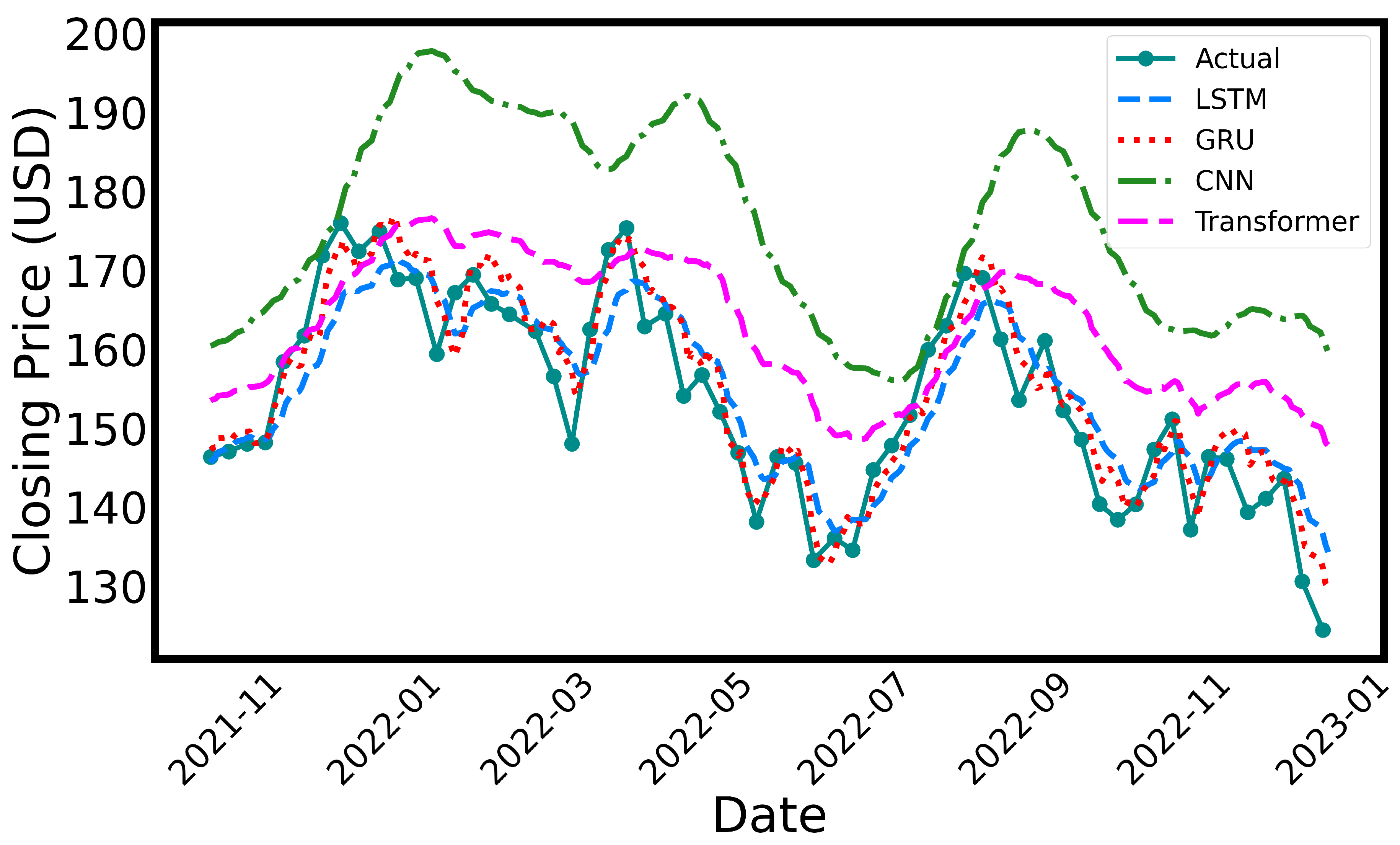
Figure 2.
Forecast comparison of univariate time-series models on daily minimum temperatures in Melbourne. The actual temperature values are sparsely plotted with markers to enhance the visibility of forecasted trends. The predictions from LSTM, GRU, CNN, and Transformer models are visualized using dash-dotted line style and colors for clarity. All models were trained using a 30-day input window and evaluated on the same test dataset from mid-1989 to late 1990.
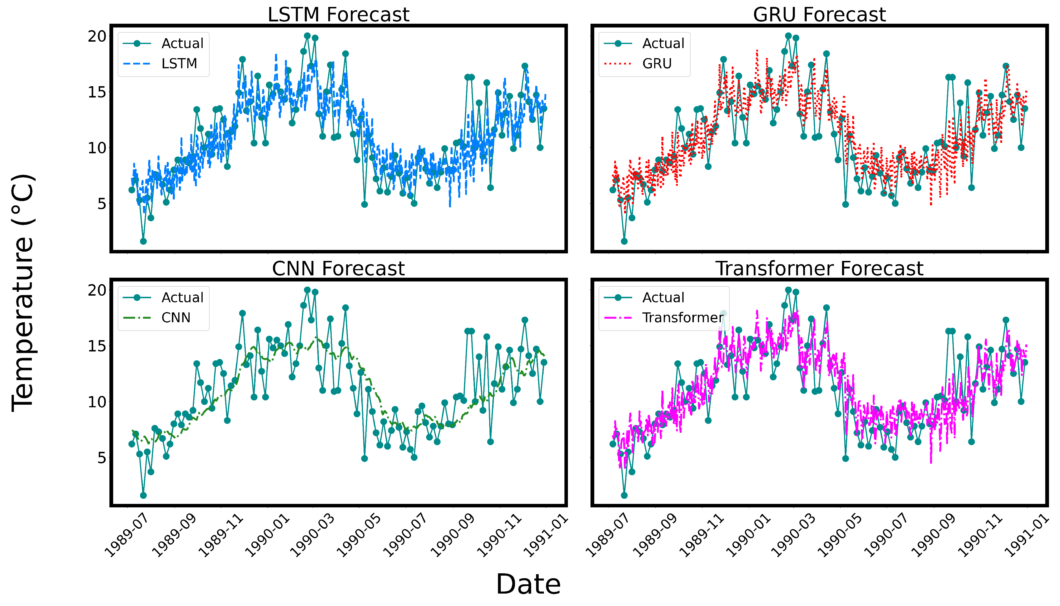

Table 1.
Forecasting performance comparison on Apple stock (AAPL) price test dataset.
| Model | MAE (USD) | RMSE (USD) | MAPE (%) |
|---|---|---|---|
| LSTM | 9.7333 | 11.6148 | 6.0979 |
| GRU | 3.2319 | 4.0355 | 2.1485 |
| CNN | 20.1176 | 22.6657 | 13.4692 |
| Transformer | 20.1454 | 21.0214 | 13.2451 |
Table 2.
Forecasting performance comparison on daily minimum temperature in Melbourne, Australia test dataset
Table 2.
Forecasting performance comparison on daily minimum temperature in Melbourne, Australia test dataset
| Model | MAE (°C) | RMSE (°C) | MAPE (%) |
|---|---|---|---|
| LSTM | 1.7338 | 2.2242 | 19.5087 |
| GRU | 1.7343 | 2.2184 | 19.8517 |
| CNN | 1.9451 | 2.5403 | 21.8412 |
| Transformer | 1.7481 | 2.2630 | 20.1516 |
Disclaimer/Publisher’s Note: The statements, opinions and data contained in all publications are solely those of the individual author(s) and contributor(s) and not of MDPI and/or the editor(s). MDPI and/or the editor(s) disclaim responsibility for any injury to people or property resulting from any ideas, methods, instructions or products referred to in the content. |
© 2026 by the authors. Licensee MDPI, Basel, Switzerland. This article is an open access article distributed under the terms and conditions of the Creative Commons Attribution (CC BY) license (http://creativecommons.org/licenses/by/4.0/).
Copyright: This open access article is published under a Creative Commons CC BY 4.0 license, which permit the free download, distribution, and reuse, provided that the author and preprint are cited in any reuse.


