
Submitted:
25 January 2026
Posted:
26 January 2026
You are already at the latest version
Abstract
Experimental and simulation studies on fluid transport system are seldom discussed in the open literature. Nevertheless, the insights and data derived from such research can significantly mitigate the scarcity of health data from real-world systems, thereby facilitating the development of advanced physics-based and data-driven algorithms. This study employs a test rig located at the IVHM Centre, Cranfield University, for experimental investigations. Based on the experimental results, an almost entirely data-driven simulation model was developed. Additionally, a case study was conducted to validate the capability of the developed simulation model and its benchmark data in supporting the creation of machine learning based fault diagnosis algorithms. The findings from this work have potential applications for a broad audience, including researchers and scholars in the fields of fluid transport system analysis, fault diagnosis, and data-driven classification algorithms.
Keywords:
fluid transport system
; fault diagnosis
; experiment
; simulation model
; health monitoring
; benchmark dataset
; machine learning
1. Introduction
Reliable and optimised Integrated Vehicle Health Management (IVHM) solutions are essential for improving system availability and reducing maintenance costs in high-value, high-technology assets. This paper presents the development of a Fluid Transport System (FTS) test rig and a corresponding simulation model constructed using experimental data from the rig. The simulation model enables efficient data collection under various health conditions and provides a robust platform to support data-driven IVHM research.
To demonstrate its capability, a case study was conducted in which simulated data were used to train several machine learning algorithms for system fault diagnosis. The results confirm that the developed simulation model effectively supports diagnostic analysis and facilitates the implementation of predictive maintenance strategies.
The remaining sections of this paper are organised as follows: Section 2 provides a systematic introduction to the test rig utilised in this study and discusses the experimental work conducted. Section 3 outlines the primary process of modelling the fluid transport system and systematically verifies the simulation results. Section 4 introduces a case study on fault diagnosis in the simplified FTS, leveraging simulated data and a machine learning (ML) approach to demonstrate the proposed method’s applicability. Finally, Section 5 summarises this paper’s overall contributions and outlines potential future work directions.
2. FTS Experimental Work
2.1. Literature Review
Aircraft fuel systems (AFS) can be regarded as a representative class of fluid transport systems (FTS), characterised by multiple tanks, pumps, valves, and heat exchangers operating under a wide range of environmental and load conditions [1]. Fault diagnosis in such systems poses similar challenges to those encountered in other complex fluid transport applications. For this reason, studies on AFS provide valuable insights and are reviewed here as representative work in the broader field of FTS fault diagnosis.
Several test rigs are documented in the following literature, which were specifically designed to study AFS fault diagnosis. Among the selected studies, Ref. [2] and Ref. [3] primarily focus on the influence of temperature on the performance and reliability of AFS components. These works centre around test rigs designed to simulate specific thermal conditions to evaluate system behaviour.
First, an icing test rig was developed to evaluate the performance of an AFS under supersaturated water conditions [2]. The rig included key components such as fuel tanks, pumps, a heat exchanger, a filter, and valves, with instruments installed to monitor water content, temperature, pressure, flow rate, and fuel levels. Liquid nitrogen was used to create a low-temperature environment for fuel cooling. To closely replicate real-world icing behaviour, the fuel tank structure, pipeline materials, and dimensions matched those of an actual AFS. Highly water-saturated fuel was used, adding additional water to intensify test conditions. The study also detailed a strict fuel preparation process, circulating and cooling the fuel to the target temperature at a controlled cooling rate.
Research was further extended into the high-temperature domain, where a test rig was employed to validate methods for suppressing cavitation in a piston pump, a critical component of aircraft engine fuel control systems [3]. Cavitation, caused by fuel suction and discharge at elevated temperatures, was addressed using a setup that included a piston pump, valves, a filter, a cooler, and various sensors for pressure, temperature, and flow. A throttling valve and a cooler were used in combination to maintain the fuel at a precise temperature of 333 K.
Ref. [4] and Ref. [5] focus on developing and testing control systems for AFS. These studies emphasise system behaviour under various operating conditions and faults, leveraging simulation or intelligent control frameworks to enhance robustness and performance.
One approach investigated the application of transfer learning for fault-tolerant control, demonstrated using a six-tank fuel transfer system originally removed from an aircraft wing [4]. Fuel was pumped between tanks to maintain mass balance around the aircraft’s longitudinal axis, even when system faults such as valve closure failures or pump leakage occurred.
Another study examined the fuel and control systems of a gas turbine engine using a hardware-in-the-loop (HIL) test rig capable of simulating steady-state and transient performance under both closed- and open-loop configurations [5]. The setup incorporated multiple full-scale fuel system components to replicate realistic system environments, including fuel pumps, tanks, metering units, a cooling system, and a large industrial computer-based control station. Additionally, the test rig was installed in an altitude-temperature chamber and mounted on a shaking table to simulate various operating conditions. Compared to Ref. [4], the inclusion of such equipment allowed for a more accurate reproduction of real flight conditions, enhancing the fidelity and applicability of the test results.
2.2. Limitation of Full-Scale Rigs
These examples illustrate the broad applicability and flexibility of test rigs in advancing research on AFS fault diagnosis. However, using actual system components and hazardous fluids (e.g., flammable or toxic fluid) in laboratory environments can pose significant challenges regarding cost, safety, environmental impact, and maintenance. In contrast, simplified test rigs that use safer working fluids such as water can not only reduce operational risks but also meet the accuracy and repeatability requirements of fault diagnosis research [1].
According to the systematic discussion of fuel system experimental work in Ref. [1], scaled-down or simplified test rigs offer significant advantages over full-scale test rigs (or actual systems) in terms of efficiency, cost, reproducibility, and flexibility. For example, intermittent fault diagnosis was studied using a simplified test rig, which included an external gear pump, a filter, two tanks, shut-off valves, check valves, a three-way valve, and several direct-acting proportional valves (DPVs) [6]. These DPVs allowed the simulation of a wide range of fault types, including incipient, slow progression, cascading, abrupt, and intermittent failures. The test rig was demonstrated to be effective in supporting fault detection and isolation (FDI) requirements.
2.3. Cranfield Rig History and Current Design
2.3.1. Rig History
The test rig used in this study is in the IVHM Laboratory at Cranfield University. Its development began in 2012 when Ref. [7] designed an initial version to emulate a UAV fuel system. In 2017, Ref. [8], significantly enhanced the rig by adding components, transducers, and flow paths, thereby improving its overall functionality and usability. Water was chosen as the working fluid for experimental simplicity and safety. To date, this rig and the datasets it has produced have supported numerous studies [9,10,11,12,13,14], and the use of water as a substitute has been shown not to alter the fundamental methodology or logic of the experimental and simulation-based research. In this paper, the existing rig has been reconfigured to capture the key operational characteristics of the FTS, providing a robust and representative platform for the current investigation.
The test rig meets several key requirements:
- Simulating the FTS under normal and faulty conditions. All associated failure modes should be able to be controlled independently and simultaneously.
- Allowing researchers to measure representative metrics (e.g. static pressure and flow rate) at any key points.
- Simulating different degraded levels for each failure mode and responding quickly. The fault configuration can be automatically adjusted for repeated experiments, and the corresponding data should be collected efficiently.
2.3.2. Current Design
As previously stated, the AFS is a representative example of the FTS. Accordingly, the design of the test rig was guided by the major components and connection topology of an AFS. Figure 1 illustrates the schematic diagram of a partial Boeing 777 fuel system, focusing on the main engine feed line. The left section of the diagram represents the airframe fuel system, located within the fuselage and wing box, responsible for boosting fuel from the fuel tank to the main engine. The right section depicts the engine fuel system, situated within the main engine, where it pressurises the fuel and regulates the fuel supply. This rig was reconfigured to encompass the feed line from the tank to the injectors and includes several critical components along this line, such as the boost pump, flow meter, Heat Exchanger (FOHE), and nozzle.
The actual test rig and its corresponding schematic are shown in Figure 2 and Figure 3, respectively. The main components are labelled from 1 to 8 in both figures for straightforward cross-reference, and a table in Figure 2 lists the component names associated with each label. Among the three gear pumps shown in Figure 2, only one (Component 2) is connected to the fluid circuit; the remaining pumps allow the test rig to be further extended in future studies as experimental needs evolve. Additionally, the working fluid recirculates back to the same tank (Component 1) after passing through the system, ensuring continuous operation under a constant tank level and inlet pressure. A narrower pipeline (Component 6) is used to represent the FOHE, capturing its dominant effect—namely, the significant pressure drop—while simplifying its internal geometric details.
The fluid power source of the test rig is an Oberdorfer-N999R external gear pump. This pump features two spur gears, each with 12 teeth, and can operate at speeds of up to 1750 rpm and flow rates of up to 28 L/min. It is mechanically driven by a 370 W Romatec motor, and the combined shaft speed is monitored using a Pepperl+Fuchs laser sensor. The recorded signal is logged in the data file and further employed as a feedback variable in the control system.
Flow perturbations are introduced through Direct Proportional Valves (DPVs), which are normally closed solenoid valves achieving full opening at a 10 V command. Owing to their low loss, low hysteresis, and high sensitivity, DPVs provide a precise and repeatable means of simulating faults within the pipeline. Five DPVs are integrated into the system: two (DPV 3 and DPV 5) are installed along the main pipeline to emulate partial blockages, while three (DPV 1, 2, and 4) are mounted on side branches to represent leakages. Each DPV responds proportionally to the input voltage, enabling continuous control of fault severity—where leakage corresponds to partial opening and blockage to partial closure. For example, a 20% leakage severity is simulated by applying 20% of the maximum voltage (2 V), whereas a 20% blockage severity corresponds to 80% of the maximum voltage (8 V).
System monitoring relies on multiple sensing elements. Three Omega turbine flow meters, each rated for 0.2–2 L/min, are installed along the main pipeline. One measures the suction flow entering the pump, whereas the remaining meters quantify downstream flow after external leakages. Pressure measurements are acquired at seven points using two types of IMP Industrial transducers: p1–p3 capture absolute pressure in the range 0–5 bar, and p4–p7 capture gauge pressure in the range 0–4 bar. Pump speed is independently confirmed by the laser sensor.
The working fluid is conveyed through a polyurethane pipeline (6 mm outer and 4 mm inner diameter), which preserves a constant cross-sectional geometry under applied pressure.
The control architecture, illustrated in Figure 2, integrates five National Instruments module cards distributed across two NI CDAQ-9172 USB chassis interfaced with a host computer. These modules handle bidirectional signal exchange, transmitting control commands to the motor and DPVs, while simultaneously acquiring analogue (voltage) and digital (pulse) signals from the sensors. Data acquisition and supervisory control are implemented in LabVIEW through a dedicated graphical interface, enabling automated operation of the pump/motor, adjustment of DPV openings, and continuous logging of measurement data.
The complete rig is mounted on an aluminium breadboard housed within a steel tray. This configuration facilitates rapid reconfiguration while ensuring safe containment of fluid spillage.
2.3.3. List of Possible Faults
Table 1 summarises the failure modes selected for this study and details the corresponding DPVs replicating these faults. Figure 2 depicts the location of these components in the test rig. Notably, the list of failure modes can be expanded, as the test rig is designed to be highly reconfigurable to accommodate additional scenarios.
Pump malfunctions are classified as external or internal leakage. External leakage refers to unintended fluid escape from the pump to the environment, typically caused by seal or casing damage, compromising performance, efficiency, and safety. Internal leakage occurs when fluid recirculates within the pump due to worn components or imperfect assembly, leading to reduced discharge pressure and flow rate.
To simulate these failures, a side pipeline branching from the main line is used, controlled by DPV1 and DPV2. External leakage is emulated by diverting part of the pump output to the reservoir, while internal leakage is represented by routing fluid from the outlet back to the inlet.
In the heat exchanger (FOHE), failures include blockage and leakage. Blockage typically occurs at the inlet when ice or debris obstructs the narrow heat-exchange tubes, whereas leakage arises from structural failure of the thin tubes separating fluids of high temperature difference. These degradations are replicated using DPV3 at the FOHE inlet (blockage simulation) and DPV4 downstream (leakage simulation). Adjusting DPV3 and DPV4 allows controlled variation of fault severity.
The final failure mode, injector nozzle clogging, results from debris accumulation or inadequate filtration, reducing engine performance. This fault is simulated by replacing the nozzle with DPV5, enabling adjustable replication of clogging conditions.
2.4. Experimental Work
The LabVIEW GUI enables the test rig to operate under either a specified pump speed or flow rate; pump-speed control is used in this study. The GUI also provides an automated mode suitable for batch experiments, in which the rig follows a predefined sequence, duration, and set of pump and DPV operations; this mode is adopted here.
2.4.1. System Performance Checks
This section briefly summarises pre-experiment repeatability checks on the test rig. Tests were performed on a fully healthy rig over two consecutive days at five pump speeds (200–600 rpm), using only steady-state data. Repeatability was evaluated by the deviation between the two-day mean values and the corresponding local pressure or flow rate. Most sensors showed <1% deviation. The maximum pressure and flow deviations were 1.31% at p6 (600 rpm) and 1.51% at f3 (500 rpm), respectively, indicating that the rig exhibits good overall repeatability.
2.4.2. Experimental Matrix
Table 2 defines the full operational matrix of the test rig, comprising 15,625 configurations generated from five DPVs, each with five degradation severities, combined with five pump speeds. This matrix represents all five failure modes and their associated degradation states.
Before the experiment, 6,000 points were randomly sampled from the full matrix. Simple random sampling was adopted to obtain an unbiased and representative subset of the operating space, while keeping the total experimental workload and data volume at a practical level. This sample size provided sufficient coverage of the system’s behaviour while reducing the required physical experimentation time and avoiding significant performance degradation of the test-rig components.
During the experiment, each selected health condition was applied once to the test rig, with each configuration completed within a few seconds. High-frequency sensor data were collected throughout to capture detailed system responses for subsequent analysis.
2.4.3. Experimental Results
The pressure sensors and flow meters sampled at 1 kHz for 13 seconds in each experiment, with 10 seconds for settling and 3 seconds for data collection. The settling period ensured completion of health-condition switching and restoration of steady flow, verified experimentally. The subsequent 3 seconds yielded 3,000 raw samples per sensor for analysis.
Figure 4 shows the unaveraged steady-state data from the 14th experiment; as noted in Section 2.4.2, 6,000 such datasets were collected in total. Sensors are colour-coded, and the corresponding health condition is listed in the figure. Key observations include:
- Flow meters exhibit more outliers than pressure sensors.
- Under steady state, all signals fluctuate within bounded ranges due to pump internals, flow dynamics, and vibration.
- Pressure sensors near the pump outlet (p3, p4, p5) show clear periodicity: ten cycles over 3 seconds, matching the pump’s gear-rotation count. A shorter window (Figure 5a) highlights suction (p2) and discharge (p4) pressure ripples associated with the 12-tooth gear.
- The frequency spectrum (Figure 5c) confirms that the gear-meshing frequency (40 Hz) dominates the suction-side signal. For discharge pressure (Figure 5b), rotational effects are evident, but individual tooth-meshing pulses are less pronounced; the spectrum contains harmonics of the rotational speed, with the meshing frequency also present.
The 3,000 samples from each sensor were then averaged and processed as described next.
Given that local atmospheric pressure (pbarometer) fluctuates over time, Equations 1 and 2 normalise the absolute and gauge pressure measurements from different days to a common reference corresponding to the standard atmospheric pressure (pSTP). After normalisation, the data are reorganised into component-level characteristic data. These data will later be illustrated using the gear pump (Figure 7) and DPV 3 (Figure 8), where each data point corresponds to the result of a single experiment.
2.5. Summary and Contribution of the Experimental Dataset
The experiments conducted in this study yield a comprehensive health monitoring dataset for a simplified yet representative fluid transport system. A key contribution of this work is that the resulting data correspond directly to physically interpretable mechanisms—such as blockage, leakage, pressure, and flow rate—rather than abstract or unspecified fault conditions commonly found in existing open-source datasets. The measurements therefore possess clear engineering relevance, enabling a more meaningful linkage between component-level degradation and system-level response.
By providing data across a wide range of well-defined health conditions, this dataset helps address the current lack of publicly accessible health data for fluid transport systems. It offers a foundation for future studies in both physics-based system simulation and the development and benchmarking of data-driven diagnostic algorithms.
The following chapters demonstrate how this dataset can be utilised for these purposes, illustrating its value for supporting modelling, analysis, and diagnostic methodology development.
3. FTS Simulation for Normal and Abnormal Conditions
3.1. Introduction
Ref. [1] provides a comprehensive review of recent simulation studies on AFS—one class of FTS—and highlights the central role of Simulink in developing both steady-state and dynamic models, including 0-D (time-dependent) and 1-D (spatially varying) representations.
As part of the Simulink environment, Simscape offers a library of physical components and simulation tools well suited for modelling real-world systems [17]. It converts governing equations into physical blocks, enabling users to construct models through drag-and-drop operations [18] without handling complex mathematical expressions [19], and allows models to be extended across domains [20]. Owing to its verified and well-maintained libraries, Simscape often yields lower modelling effort and faster development than traditional Simulink implementations [21,22]. When built-in components are insufficient, Simscape also supports modifying existing libraries or creating custom ones [23], making it particularly suitable for simulating the test rig in Section 2. For this reason, Simulink Simscape is selected as the simulation platform in this work.
Simscape has been widely applied to mechanical [24], hydraulic [19,25,26,27], and thermo-fluid systems [18,28,29,30], supporting both kinematic and dynamic analyses [17] as well as fault-diagnosis research [31,32]. For example, Simscape Fluids has been used to model AFS and analyse their behaviour under different operating conditions and fault scenarios [31]. In another study, a hydraulic pump-centred system was modelled to output power, flow rate, and pressure, with simulated pump characteristics closely matching experimental data [33].
A Simscape-based fuel-system model for a gas-turbine engine was further developed to evaluate performance metrics such as power consumption and energy losses under various operating conditions [34]. This model captured transient behaviour, supported closed-loop control, and demonstrated scalability for adaptation to different system configurations. Simscape has also been used to construct digital twins of fluid-system pumps for training fault-diagnosis algorithms via transfer learning, generating simulation data where experimental fault signals are limited [35]. Its modularity also enables rapid updates when component properties change.
In another study, custom Simscape libraries have been developed for pressure sensors and integrated into multi-domain simulations involving electrical, mechanical, and fluid interactions [36]. Simscape has also been selected for modelling the environmental control system (ECS) of a Boeing 737-800 due to its user-friendly interface, computational efficiency, and flexibility [32]. A dedicated library, “Simscape ECS Simulation under All Conditions” (SESAC), was established and validated against real-world data.
3.2. Simulation Model
The simulation model shown in Figure 6 reproduces the test rig (Figure 3) using the Simulink Simscape environment. The model includes six controllable elements: a fixed-displacement pump with five speed settings and five 2-way directional valves (DPVs) used to introduce different fault severities via variable openings. This configuration yields up to 15,625 unique health-condition combinations, and the resulting steady-state pressure and flow rate data form the basis for the subsequent fault-diagnosis study.
Figure 6.
Simulation model in Simulink.
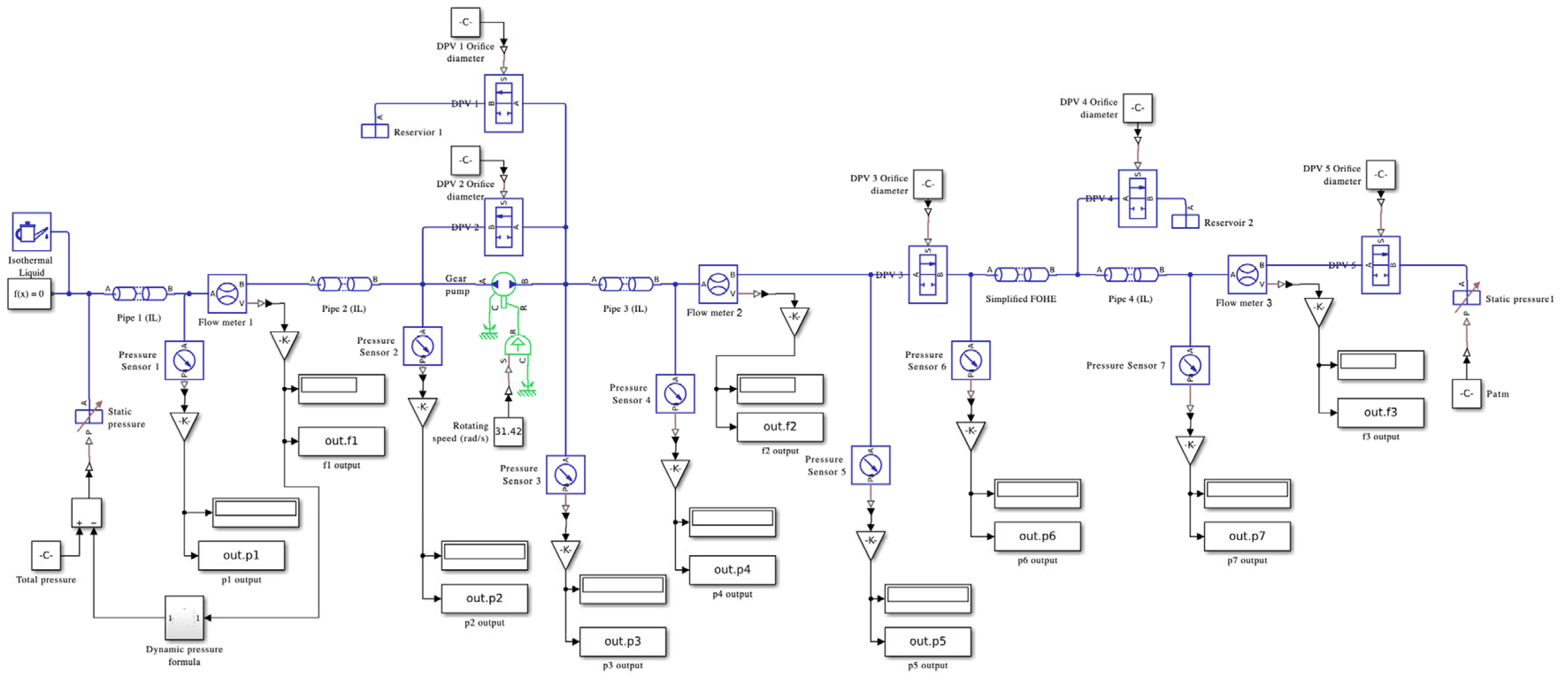
Because the model includes multiple unknown pressures and flow rates, it is essential that the number of equations matches the number of unknowns to form a solvable system. Table 3 summarises all unknowns and their corresponding governing “equations.” Except for the Bernoulli equation, all relationships are derived directly from experimentally obtained component characteristics—such as the dotted curves in Figure 8 for the DPVs—making the model a data-driven simulation.
In this formulation, pressures are determined from the boundary conditions and the characteristic curves of each component. The inlet flow rate from the tank is calculated using Bernoulli’s equation (Equation 3), ensuring conservation of total head. Applied at the entrance of the main pipeline, the left-hand side represents the total pressure at the bottom of the tank, which includes the hydrostatic component associated with depth (d). The right-hand side corresponds to the static pressure (pₛ) at the inlet and the dynamic pressure associated with the inlet velocity (v). The velocity is expressed in terms of volumetric flow rate Q via Equation 4, where A is the pipeline cross-sectional area.
The pressure–flow characteristics used in the simulation, shown as the dotted curves in Figure 7 and Figure 8, are obtained by reorganising the experimental data from Section 2 into pressure-drop versus flow rate relationships for each component. These characteristics are then used as inputs to the simulation model, providing Simscape with a complete equation set for steady-state solutions.
Figure 7 presents the pump characteristic curves, describing the relationship between flow rate and pressure rise. As downstream backpressure increases (e.g., due to a partially closed valve), the pump delivers lower flow but higher pressure-rise. To avoid excessive mechanical stress and prevent expansion of the plastic tubing, the operating speed was limited to 600 rpm during experiments. Experimental points are plotted as dots, showing increased data variability at higher speeds. Although the trends remain consistent across speeds, higher pump speeds produce greater pressure rise for the same flow rate. Because the experimental data fall within a narrow range, smoothed curves were extrapolated to cover a broader interval, enabling robust simulation across wider operating conditions. Pump degradation would shift the curve downward, but Figure 7 accurately reflects the pump behaviour during the experiments in this study.
Figure 7.
Pump experimental data and characteristics.

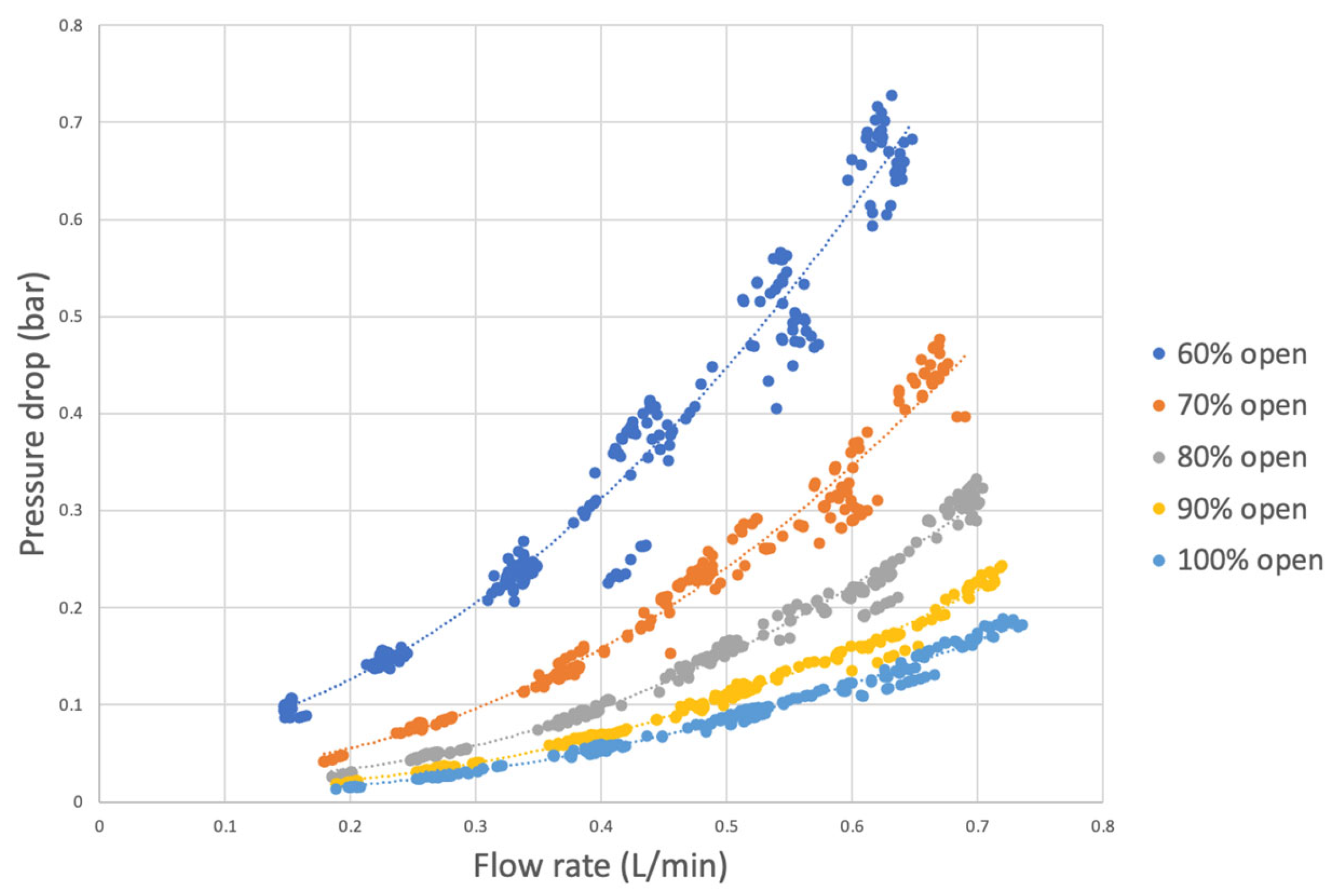
Beyond the pump, three additional components—DPVs, pipelines, and the FOHE—contribute to system backpressure and shape the overall operating point. Their behaviours are modelled individually. Adjusting the opening of each DPV alters the flow resistance: smaller openings generate higher upstream backpressure and larger pressure drops. Figure 8 shows the characteristic curves for five opening positions, each with experimental points (dots) and smoothed curves (dotted lines) used in the simulation. Across all openings, higher flow rates correspond to larger pressure drops.
Figure 8.
Experimental DPV characteristics (DPV 3).
Pressure losses in the pipeline network were experimentally confirmed to be non-negligible and are therefore incorporated into the model. The pipelines are divided into three sections—upstream of the pump, between the pump and Flowmeter 2, and downstream of the FOHE. Each section exhibits similar monotonic behaviour: greater flow rates cause greater pressure drops, with the curves scaled according to pipe length.
The FOHE is represented experimentally by a small-diameter pipe (ID = 2.6 mm) with multiple bends, mimicking typical internal heat-exchange channels. This structure imposes substantial resistance compared with straight pipelines and is modelled using a single characteristic curve with significantly higher pressure drop at any given flow rate.
External leakages can also be simulated. The leakage flow rate is determined from the local pressure difference and the leakage characteristic data, while downstream flow rates follow from mass-conservation constraints. With two possible leakage points, the model can output up to three distinct flow rates.
3.2.1. Simulation Results - Healthy Condition
Having established the simulation model, this section presents its validation at both the component and system levels. The model was validated at two levels: component level and system level. At the component level, the output behaviour of each element was checked against its characteristic curves, confirming that the implemented components operated as expected. System-level validation then examined whether the simulation model reproduced the behaviour observed in the test rig.
To verify the integrity of the simulation model, it was first evaluated in a fully healthy state across all pump speeds. The simulated outputs were compared with the corresponding experimental measurements, ensuring that the main pipeline and component connections were correctly represented.
Figure 9 presents the comparison between the model and the experimental data. The top two plots show pressure (Figure 9a) and flow rate (Figure 9b), where simulation results are plotted using dashed lines and experimental data using solid lines. Five colours represent the five pump speeds.
In the pressure plot, the progression from p1 to p7 follows the expected physical trend. Pressure decreases from atmospheric pressure at the inlet to the pump suction point (p2), rises sharply across the pump to the outlet (p3), and then gradually decreases along the downstream pipeline back to atmospheric conditions.
The flow rate plot shows that the pump draws a flow rate that increases approximately linearly with pump speed, consistent with the system’s expected behaviour.
The relative difference between experiment and simulation is quantified using Equation 5, with results shown in Figure 9c and Figure 9d. Most pressure and flow rate deviations fall within ±1.6%. The maximum flow rate deviation is −3.3% at 200 rpm, indicating a slightly higher simulated flow rate relative to the experiment. These discrepancies are partly attributable to the fact that the simulation model considers only the three main pipeline sections of the test rig, whereas the real system contains additional minor pipework and fittings that introduce extra losses. Moreover, measurement uncertainty in the flow meters becomes more pronounced at low pump speeds, which likely amplifies the deviation observed at 200 rpm. As the system is in a healthy state, the differences shown in Figure 9 serve as the baseline for the validation analyses presented in the next section.
3.2.2. Simulation Results - Faulty Conditions
Five faulty scenarios at different pump speeds were used to validate the simulation model under degraded conditions. The first two scenarios examine blockage in the main pipeline, while the remaining three evaluate the model’s ability to reproduce external and internal leakages introduced through the three side pipelines.
Figure 10 presents the percentage gaps between the simulated and experimental results. For pump external leakage (DPV1), both pressure and flow rate show noticeable discrepancies, although they remain within an acceptable range (<1.5%). Larger pressure deviations appear in the FOHE leakage (DPV4) and pump internal leakage (DPV2) scenarios, which are likely attributed to inaccuracies in the characteristic data used as model inputs.
Leakage simulation requires input data that reflect the actual leakage rates observed during the experiments. These leakage rates are obtained by combining measurements from Flowmeter 2 and Flowmeter 3 (pump external leakage = f1 – f2; FOHE leakage = f2 – f3). This processing effectively doubles the flow-measurement uncertainty in the leakage region, which in turn affects the agreement between the simulated outputs and the experimental data.
To reduce these discrepancies, the model can be reconfigured to operate with prescribed flow rates rather than pump speeds by replacing the pump block with a fluid source. Under this setup, the pump no longer influences the system behaviour; instead, all outputs depend solely on the boundary conditions (atmospheric pressure), and the pressure drops of the remaining components. Although this reduces the number of unknowns and equations by one, the system remains solvable. Bernoulli’s equation is then applied to calculate the inlet static pressure based on the known flow rate.
Figure 11 summarises the validation results obtained using flow rate-matched simulations. In most cases, the percentage gaps are significantly reduced, apart from the clogged-nozzle scenario (blue line). This suggests that variations in pump behaviour between experiments can affect the model’s accuracy when pump-speed control is used.
The red line in Figure 11 further indicates that the side-pipeline configuration for simulating FOHE leakage requires refinement. As noted earlier, improving the accuracy of the input characteristic data is a promising direction for enhancing the reliability of the leakage simulation.
3.3. New Benchmark Dataset
To ensure comparability between the experimental and simulated results, the simulation model was executed 6,000 times using the same combinations of health conditions and the same random seed as in Section 2.4.2. Although the model can simulate many more operating conditions, this configuration reproduces the benchmark dataset. Unlike the continuous high-frequency sampling on the test rig, the virtual sensors in the simulation provide a single steady-state output for each run.
Figure 12 presents the resulting dataset for single-component degradations across five severity levels and illustrates their effects on system behaviour. Each subfigure corresponds to one failure mode, with line plots showing the pressure distribution throughout the system and colour-coded degradation levels. The accompanying table reports the percentage of flow rate under each health condition relative to the fully healthy state.
Across all failure modes, the flow rate decreases as degradation progresses. The reduction is modest at low severity but becomes much more pronounced once a threshold is exceeded.
From a pressure-distribution perspective, FOHE blockage (Figure 12c) and clogged nozzles (Figure 12e) increase upstream pressure due to pump backpressure, thereby reducing the system flow rate in accordance with the pump’s characteristic curve. In contrast, external leakages at the pump (Figure 12a) or FOHE (Figure 12d) slightly lower system pressure. FOHE leakage has minimal effect on pressure and flow because it occurs far downstream, making it difficult to detect; however, it still reduces the flow rate in the main pipeline while causing the pump to draw more water from the tank due to reduced backpressure.
Pump internal leakage (Figure 12b) introduces reverse flow from the outlet to the inlet, reducing pump efficiency and limiting its suction capability. Unlike blockage faults, which increase pressure, internal leakage substantially diminishes the pump’s boosting effect. As a result, a degraded pump operating at 400 rpm behaves similarly to a healthy pump at a much lower speed, making this fault challenging to detect through pressure or flow measurements alone.
Figure 13 extends the analysis to FOHE blockage combined with additional degradations (multi-component scenarios). These compound faults further reduce the flow rate relative to the single-fault case in Figure 12c. However, system pressures may diverge from the single-degradation baseline, decreasing when leakage is present or increasing when nozzle clogging co-occurs.
A notable observation is that the pressure traces for different FOHE blockage levels no longer form five clearly separated lines as in Figure 12. Instead, they appear as overlapping bands of values. This overlap reduces the distinguishability of FOHE blockage severity and indicates that additional degradations can significantly obscure fault signatures, complicating the identification of degradation levels.
3.4. Summary of the Simulation Model
The simulation model developed in this section helps address the shortage of open-source models for fluid transport systems (FTS) and reproduces, in a repeatable manner, the data-generation capability of the test rig described in Section 2. As the second major component of this work, the simulation model serves as a bridge between the experimental dataset and the data-driven algorithms. It reduces the variability inherent in physical testing and enables the efficient generation of sufficient health-monitoring data at a much lower cost than hardware-based experiments. Simulation of abnormal conditions can also generate large-scale datasets for training machine-learning algorithms, especially when experimental testing is limited or impractical; however, modelling errors may influence diagnostic performance.
The model’s performance was evaluated by quantifying the percentage differences between simulated outputs and experimental measurements. For healthy conditions at higher pump speeds, the agreement is satisfactory, with errors below 2%. At the lowest pump speed (200 rpm), the discrepancies are larger but remain within 4%. These differences are likely attributable to limitations in the test-rig sensors—particularly the flow meters—which do not capture low-flow behaviour with high fidelity, as well as interpolation and extrapolation errors introduced during data processing. Under faulty conditions, the model shows consistently poor performance when simulating FOHE external leakage. This is again linked to insufficiently accurate experimental data, which do not fully capture system behaviour under small leakage rates, leading the model to overestimate the pressure losses associated with this fault mode.
These observations highlight a key limitation of data-driven simulation models: their accuracy is highly sensitive to the quality of the input data, in contrast to equation-based simulations. Improving model fidelity therefore requires improving the quality of the experimental data. For the test rig described in Section 2, future enhancements may involve replacing the current flow meters with instruments capable of resolving low flow rates more accurately and repositioning the leakage-measurement flow meter to obtain more reliable leakage data.
4. Diagnostics Through Machine Learning
This section illustrates the capability of the proposed dataset to support data-driven diagnostic development. Using the simulated data introduced in Section 3.3, the example demonstrates that the dataset is suitable for training diagnostic algorithms. Several widely used AI-based approaches are evaluated for their ability to detect five fault types in the fluid transport system (FTS), including scenarios involving multi-component degradation.
4.1. Introduction
Machine learning (ML) and deep learning (DL) techniques have been increasingly adopted for fault diagnosis in a wide range of engineering domains [37,38,39,40,41]. These methods extract diagnostic information from data through mathematical modelling, enabling automated fault detection and isolation that would traditionally rely on domain expertise. This capability has attracted significant interest in applications involving complex systems such as FTS.
For example, Support Vector Machines (SVMs) and Multilayer Perceptrons (MLPs) have been used to diagnose faults in external gear pumps using simulation-generated training data [42], with the single-layer MLP outperforming the SVM. Similar findings were reported in two studies on AFS diagnostics [43,44], where neural networks demonstrated faster convergence, reduced computation time, and higher accuracy compared with SVMs.
Most classical ML approaches, however, rely on manual feature extraction, which can be difficult and often requires detailed knowledge of the underlying system [45]. In contrast, DL approaches operate directly on raw data and automatically learn hierarchical representations. This capability has motivated work such as applying 2D Convolutional Neural Networks (2D-CNNs) to fault diagnosis by converting 1D time-series signals into 2D images [46,47]. While effective, these studies also emphasise a key limitation of DL: its performance degrades sharply when training data are limited. A survey of DL applications in aviation Maintenance, Repair, and Overhaul (MRO) further shows that methods such as autoencoders, LSTMs, CNNs, and DBNs have been used for diagnosing engines, fuel systems, and actuators [48], but consistently require large, high-quality datasets.
A broader summary of AI-based diagnostic methods for FTS has been presented previously [1] and is not repeated here. Instead, five criteria were established to determine suitable algorithms for the present study:
- Feature suitability: The dataset used here consists of eleven structured features with clear physical meaning and proven sensitivity to FTS faults. As a result, complex DL methods designed for latent-feature extraction from unstructured data are unnecessary.
- Data-volume compatibility: The selected algorithms must function effectively with a training set of approximately 4,000 samples.
- Supervised learning: Since the simulated dataset is fully labelled, supervised methods are preferred.
- Classification capability: Fault diagnosis is inherently a classification problem, requiring algorithms well suited for binary or multi-class classification.
- Model complexity vs. predictive performance: The chosen algorithms should provide strong diagnostic accuracy while maintaining reasonable computational cost.
Based on these criteria, four classical ML classifiers—Logistic Regression (LR), Decision Tree (DT), Support Vector Machine (SVM), and Artificial Neural Network (ANN)—were selected. These algorithms are widely used in data-driven fault diagnosis and, importantly, each satisfies all five selection criteria. They offer strong classification capability, operate effectively with the available dataset size, and provide an appropriate balance between model complexity and predictive performance. Accordingly, they were chosen as suitable methods for training diagnostic models using the simulated data, including scenarios with multi-component degradation.
Accounting for multi-component degradation is essential for realism. In practical systems, components degrade simultaneously but at different rates, and their interactions can significantly influence diagnostic outcomes [49]. The diagnostic models developed in this study are therefore trained to recognise a specific fault mode while remaining robust to the influence of other concurrent degradations.
4.2. Data Preparation
In the data preparation stage, the dataset was randomly divided into two non-overlapping subsets for training and testing the ML classifiers. Seventy percent of the samples were allocated to the training set, and the remaining 30% to the validation set. The input features used for model training consist of seven static pressures (p1–p7), three flow rates (f1–f3), and the pump speed (RPM).
Thresholds for each failure mode (Table 4) were defined based on their observed effects on system pressure and flow rate. Degradation levels below the threshold were considered tolerable and labelled as normal, whereas those exceeding the threshold were treated as faults and labelled as abnormal. Each sample in the dataset was assigned to one of these two classes.
Figure 14 shows the influence of the five failure modes across different severity levels on the system behaviour, specifically on flow rate (Figure 14a) and on pressures in adjacent components (Figure 14b). Each group of bars corresponds to a failure mode, with degradation levels indicated above the bars (H denotes the healthy condition and 4 the most severe). Normal and abnormal conditions are highlighted in green and red, respectively. As illustrated, abnormal conditions lead to distinct and substantial performance deviations in the system.
4.3. Diagnostic Algorithm Development
i. Algorithm configuration
Logistic Regression (LR) is a statistical method commonly used for binary classification. It estimates the probability that an input belongs to a particular class by applying a sigmoid function to a linear combination of the input features. The resulting probability is compared with a predefined threshold to assign the final class label.
Decision Trees (DTs) classify samples by recursively partitioning the feature space. Each internal node represents a decision based on a specific feature, each branch corresponds to an outcome of that decision, and each leaf node denotes a class label. DTs aim to learn simple and interpretable rules that map inputs to their respective classes.
Support Vector Machines (SVMs) identify an optimal separating hyperplane that maximises the margin between classes. The method is robust to outliers near the decision boundary and can handle both linear and non-linear classification tasks using kernel functions, which map input features into higher-dimensional spaces to enhance separability.
Artificial Neural Networks (ANNs) are computational models composed of interconnected processing units (neurons). Shallow ANNs, considered here, contain an input layer, one hidden layer, and an output layer. Information is propagated through weighted connections, and these weights are iteratively updated during training to improve predictive accuracy.
Table 5 summarises the key configuration parameters for the four algorithms used in this study along with their corresponding MATLAB functions.
ii. Evaluation metrics
The performance of the classifiers was evaluated using two metrics: the confusion matrix and the F-1 score.
The confusion matrix provides a detailed summary of the classification outcomes, including true positives (TP), true negatives (TN), false positives (FP, false alarms), and false negatives (FN, missed detections), relative to the actual system state. In this study, negative denotes a normal operating condition, while positive denotes an abnormal or faulty condition.
The F-1 score, computed using Equation 6, combines precision and recall into a single metric that reflects the classifier’s effectiveness in identifying faults. As shown in Equation 6, the F-1 score does not depend on the number of true negatives, placing emphasis on detecting abnormal conditions. This emphasis is particularly appropriate when abnormal samples are much fewer than normal ones, which is the main motivation for using this metric in the present study.
iii. Algorithm assessment
Table 6 summarises the diagnostic performance and training efficiency of the four ML algorithms across the five failure modes, reported in terms of F-1 scores.
An F-1 score of 1 represents perfect classification, while a score of 0 indicates complete misclassification. All algorithms achieve F-1 scores above 0.89, indicating satisfactory diagnostic capability. Among them, the ANN yields the highest overall performance, while LR, DT, and SVM exhibit comparable results.
Blockage-related faults (FOHE blockage and Nozzle blockage) are the easiest to detect, with LR, SVM, and ANN achieving perfect identification of FOHE blockage. In contrast, Pump internal leakage is the most challenging fault type for all algorithms.
Training efficiency varies notably among the methods. ANN and DT train the fastest, whereas SVM requires substantially longer training time. Considering both accuracy and computational cost, ANN appears to be the most suitable algorithm for this application.
Figure 15 shows the confusion matrix of the trained DT model for detecting pump external leakage in the test set. The vertical axis denotes the actual labels, and the horizontal axis denotes the predicted labels, with Class 1 representing normal conditions and Class 2 representing abnormal conditions. Correct predictions are shown in blue and incorrect ones in pink, with darker shades representing higher sample counts.
Of the 343 faulty samples, the DT model correctly identifies 308 as true positives (TP) but misclassifies 35 as false negatives (FN), which may lead to undetected faults during operation. The model also produces 28 false positives (FP), which could trigger unnecessary maintenance actions and increase operational costs.
5. Summary and Conclusions
This paper presented a systematic study integrating experimental testing, data-driven simulation, and machine-learning techniques to support intelligent fault diagnosis for a fluid transport system (FTS). A machine-learning diagnostic example was also provided to demonstrate the applicability of the resulting dataset.
The IVHM test rig at Cranfield University was used to reproduce five representative failure modes of the FTS: pump external leakage, pump internal leakage, FOHE blockage, FOHE leakage, and nozzle clogging. Purpose-designed experiments were conducted to observe the individual and combined effects of these degradations and to collect corresponding health-monitoring data. Under multi-component degradation, the rig executed 6,000 unique experiments across different health conditions.
A data-driven simulation model was then developed in Simscape to replicate the steady-state behaviour of the test rig. The model uses the Bernoulli equation and experimentally derived component characteristics to generate deterministic pressure and flow rate data for the benchmark dataset without manual tuning or embedded assumptions, thereby avoiding systematic bias. Validation against experimental results across a range of health states showed a maximum deviation of approximately 3%, demonstrating good consistency between the model and the physical system.
The capability of the simulation dataset to support diagnostic algorithm development was also demonstrated. Among the four classical ML methods evaluated, a single-hidden-layer Artificial Neural Network (ANN) achieved the best diagnostic performance while requiring minimal training time, accurately identifying all five failure modes using pressure, flow rate, and pump-speed data. These results confirm the suitability of the simulation dataset for data-driven diagnostic studies.
Although the study demonstrates strong potential, further improvements are possible.
- Experimental work: Data quality could be enhanced through improved sensor placement, higher-accuracy instrumentation, and repeated trials for selected health conditions.
- Simulation work: More accurate experimental data would directly increase model fidelity. Incorporating noise and modelling transient system behaviour could also broaden the applicability of the simulation model and the datasets generated.
Finally, the diagnostic example in Section 4 focused on single-fault detection, where each binary classifier was designed to detect one specific fault. As reported in a related publication [50], the approach has since been extended to multi-fault diagnosis, enabling identification of simultaneous fault combinations within the system.
References
- Li, J.; King, S.; Jennions, I. Intelligent fault diagnosis of an aircraft fuel system using machine learning—A literature review. Machines 2023, 11(4), 481. [Google Scholar] [CrossRef]
- Liu, D.; Bian, G.; Xiao, H. The Research of Aircraft Fuel System Icing Test. In Journal of Physics: Conference Series; IOP Publishing, September 2021; Vol. 2030, No. 1, p. 012013. [Google Scholar]
- Wang, T.; Jiao, H.; Ma, X.; Ouyang, X.; Zhang, H. Analysis of Cavitation Characteristics of High Temperature Fuel Piston Pump in the Process of Suction and Discharge. In Fluid Power Systems Technology; American Society of Mechanical Engineers, October 2021; Vol. 85239, p. V001T01A026. [Google Scholar]
- Ahmed, I.; Quinones-Grueiro, M.; Biswas, G. Transfer reinforcement learning for fault-tolerant control by re-using optimal policies. In 2021 5th International Conference on Control and Fault-Tolerant Systems (SysTol); 2021, September; IEEE; pp. 25–30. [Google Scholar]
- Gafurov, S.; Rodionov, L.; Kryuchkov, A.; Handroos, H. HIL test bench for engine’s fuel control systems investigation. In 30th Congress of the International Council of the Aeronautical Sciences; 2016. [Google Scholar]
- Sedighi, T.; Foote, P. D.; Khan, S. Intermittent fault detection on an experimental aircraft fuel rig: Reduce the no fault found rate. In 2015 4th International Conference on Systems and Control (ICSC); 2015, April; IEEE; pp. 110–115. [Google Scholar]
- Niculita, O.; Irving, P.; Jennions, I. K. Use of COTS functional analysis software as an IVHM design tool for detection and isolation of UAV fuel system faults. 2012. [Google Scholar] [CrossRef]
- Lin, Y. System diagnosis using a Bayesian method. Doctoral dissertation, Cranfield University, 2017. [Google Scholar]
- Shuai, F. U.; AVDELIDIS, N. P. Health Management of Aircraft Fuel Systems: A Practical Prognostic Perspective. In 2024 11th European Workshop on Structural Health Monitoring; 2024. [Google Scholar]
- Ezhilarasu, C. M.; Skaf, Z.; Jennions, I. K. A generalised methodology for the diagnosis of aircraft systems. Ieee Access 2021, 9, 11437–11454. [Google Scholar] [CrossRef]
- Liu, H.; Zhao, Y.; Zaporowska, A.; Skaf, Z. A machine learning-based clustering approach to diagnose multi-component degradation of aircraft fuel systems. Neural Computing and Applications 2023, 35(4), 2973–2989. [Google Scholar] [CrossRef]
- Iyaghigba, S. D.; Petrunin, I.; Avdelidis, N. P. Modeling a hydraulically powered flight control actuation system. Applied Sciences 2024, 14(3), 1206. [Google Scholar] [CrossRef]
- Zaporowska, A.; Liu, H.; Skaf, Z.; Zhao, Y. A clustering approach to detect faults with multi-component degradations in aircraft fuel systems. IFAC-PapersOnLine 2020, 53(3), 113–118. [Google Scholar] [CrossRef]
- Jung, M.; Niculita, O.; Skaf, Z. Comparison of different classification algorithms for fault detection and fault isolation in complex systems. Procedia Manufacturing 2018, 19, 111–118. [Google Scholar] [CrossRef]
- Opperwall, T. J. Investigation of noise sources and propagation in external gear pumps. Doctoral dissertation, Purdue University, 2015. [Google Scholar]
- Kulpa, M. A vibrational study of gear pumps and gear pump drives; 1991. [Google Scholar]
- Ogbemhe, J.; Ramatsetse, B.; Mpofu, K.; George, O. A. Multi-Physical Modelling and Simulation of a Planar Translational Scissor Lift Mechanism for Maintenance of Rail Transmission Lines. Procedia CIRP 2024, 121, 174–179. [Google Scholar] [CrossRef]
- Agbaje, M. A., Yilgor, I., Rodrigues, V. Z., Diao, X., Smidts, C., Kapuria, A., ... & Shi, S.System design and analysis of thermal power dispatch systems for boiling water reactors. Annals of Nuclear Energy 2025, 210, 110881. [CrossRef]
- Erzan Topçu, E. PC-based control and simulation of an electro-hydraulic system. Computer Applications in Engineering Education 2017, 25(5), 706–718. [Google Scholar] [CrossRef]
- Fernandez de Canete, J.; Martin-Aguilar, J. Ship-course modeling and control using the SIMSCAPE physical modeling environment. Simulation 2021, 97(4), 247–266. [Google Scholar] [CrossRef]
- Volle, C. E. (2014). Simscape Modeling Verification in the Simulink Development Environment (No. KSCE- DAA-TN18107).
- Adamcik, F.; Bréda, R.; Kurdel, P.; Beno, V. Modeling of Changes in Flow Air Fuel E ffected by Changes in Environmental Conditions. NAŠE MORE: znanstveni časopis za more i pomorstvo 2014, 61(1-2), S40–42. [Google Scholar]
- Fischer, N. P. (2015). Simscape Modeling of a Custom Closed-Volume Tank (No. KSC-E-DAA-TN23095).
- Petrović, G. R.; Mattila, J. Mathematical modelling and virtual decomposition control of heavy-duty parallel–serial hydraulic manipulators. Mechanism and Machine Theory 2022, 170, 104680. [Google Scholar] [CrossRef]
- Suchithra, R., Das, T. K., Rajagopalan, K., Chaudhuri, A., Ulm, N., Prabu, M., ... & Cross, PNumerical modelling and design of a small-scale wave-powered desalination system. Ocean Engineering 2022, 256, 111419. [CrossRef]
- Park, C. G.; Yoo, S.; Ahn, H.; Kim, J.; Shin, D. A coupled hydraulic and mechanical system simulation for hydraulic excavators. Proceedings of the Institution of Mechanical Engineers, Part I: Journal of Systems and Control Engineering 2020, 234(4), 527–549. [Google Scholar] [CrossRef]
- Pelin, R. I.; Tița, I. Modelling and simulation of a hydraulic system used for wind turbines. In IOP Conference Series: Materials Science and Engineering; 2019, September; IOP Publishing; Vol. 595, No. 1, p. 012048. [Google Scholar]
- Dahash, A.; Mieck, S.; Ochs, F.; Krautz, H. J. A comparative study of two simulation tools for the technical feasibility in terms of modeling district heating systems: An optimization case study. Simulation Modelling Practice and Theory 2019, 91, 48–68. [Google Scholar] [CrossRef]
- Fux, S. F.; Mohajer, B.; Mischler, S. A Comparison of the Dynamic Temperature Responses of Two Different Heat Exchanger Modelling Approaches in Simulink Simscape for HVAC Applications; SIMULTECH, 2023; pp. 417–424. [Google Scholar]
- Mandal, N. K.; Azad, A. K.; Rasul, M. G. On students learning experience of fluid power engineering–Impact of simulation software. International Journal of Mechanical Engineering Education 2024, 52(2), 143–156. [Google Scholar] [CrossRef]
- Mazzitelli, L.; Watanabe, P.; Teixeira, J. C.; Machado, J. A simulation model for small aircraft fuel system design. Technologia i Automatyzacja Montażu 2023, (4), 28–37. [Google Scholar] [CrossRef]
- Jennions, I.; Ali, F.; Miguez, M. E.; Escobar, I. C. Simulation of an aircraft environmental control system. Applied Thermal Engineering 2020, 172, 114925. [Google Scholar] [CrossRef]
- Kamarudin, M. N.; Rozali, S. M.; Aras, M. S. M.; Hairi, M. H.; Abdullah, L.; Rizman, Z. I. Studies on Hydraulic Pump Characteristics Through Experiment and Simulation in MATLAB Simscape. Applications of Modelling and Simulation 2024, 8, 301–309. [Google Scholar]
- Sciatti, F.; Tamburrano, P.; De Palma, P.; Distaso, E.; Amirante, R. Detailed simulations of an aircraft fuel system by means of Simulink. In Journal of physics: Conference series; IOP Publishing, December 2022; Vol. 2385, No. 1, p. 012033. [Google Scholar]
- Wang, J.; Zhang, Z.; Liu, Z.; Han, B.; Bao, H.; Ji, S. Digital twin aided adversarial transfer learning method for domain adaptation fault diagnosis. Reliability Engineering & System Safety 2023, 234, 109152. [Google Scholar] [CrossRef]
- Delhaye, T. P.; Francis, L. A.; Flandre, D.; Cretu, E. Macro-Modeling Library in Simscape for MEMS Pressure Sensors Based on Energy-Flow Paradigm. In 2019 Symposium on Design, Test, Integration & Packaging of MEMS and MOEMS (DTIP); 2019, May; IEEE; pp. 1–5. [Google Scholar]
- Amare, D. F.; Aklilu, T. B.; Gilani, S. I. Gas path fault diagnostics using a hybrid intelligent method for industrial gas turbine engines. Journal of the Brazilian Society of Mechanical Sciences and Engineering 2018, 40(12), 578. [Google Scholar] [CrossRef]
- Ravikumar, K. N.; Yadav, A.; Kumar, H.; Gangadharan, K. V.; Narasimhadhan, A. V. Gearbox fault diagnosis based on Multi-Scale deep residual learning and stacked LSTM model. Measurement 2021, 186, 110099. [Google Scholar] [CrossRef]
- Wang, S.; Fan, S.; Chen, J.; Liu, X.; Hao, B.; Yu, J. Deep-learning based fault diagnosis using computer-visualised power flow. IET Generation, Transmission & Distribution 2018, 12(17), 3985–3992. [Google Scholar]
- Park, S. Y.; Ahn, J. Deep neural network approach for fault detection and diagnosis during startup transient of liquid-propellant rocket engine. Acta Astronautica 2020, 177, 714–730. [Google Scholar] [CrossRef]
- Hamdaoui, H.; Ngiejungbwen, L. A.; Gu, J.; Tang, S. Improved signal processing for bearing fault diagnosis in noisy environments using signal denoising, time–frequency transform, and deep learning. Journal of the Brazilian Society of Mechanical Sciences and Engineering 2023, 45(11), 576. [Google Scholar] [CrossRef]
- Lakshmanan, K.; Tessicini, F.; Gil, A. J.; Auricchio, F. A fault prognosis strategy for an external gear pump using Machine Learning algorithms and synthetic data generation methods. Applied Mathematical Modelling 2023, 123, 348–372. [Google Scholar] [CrossRef]
- Jiao, X.; Jing, B.; Huang, Y.; Li, J.; Xu, G. Research on fault diagnosis of airborne fuel pump based on EMD and probabilistic neural networks. Microelectronics Reliability 2017, 75, 296–308. [Google Scholar] [CrossRef]
- Xiangyang, S. Research on fault diagnosis of B737 aircraft fuel system based on improved BP neural network. Mathematical Models in Engineering 2019, 5(1), 11–16. [Google Scholar] [CrossRef]
- Sepulvene, L., Drummond, I., Kuehne, B., Frinhani, R., Leite Filho, D., Peixoto, M., ... & Batista, B.Performance evaluation of machine learning techniques for fault diagnosis in vehicle fleet tracking modules. The Computer Journal 2022, 65(8), 2073–2086. [CrossRef]
- Ruan, Y.; Zheng, M.; Qian, F.; Meng, H.; Yao, J.; Xu, T.; Pei, D. Fault detection and diagnosis of energy system based on deep learning image recognition model under the condition of imbalanced samples. Applied Thermal Engineering 2024, 238, 122051. [Google Scholar] [CrossRef]
- Guo, Y.; Chen, X.; Wang, W. Fault diagnosis of fuel pump based on wavelet denoising and deep learning. In Journal of Physics: Conference Series; IOP Publishing, March 2022; Vol. 2216, No. 1, p. 012050. [Google Scholar]
- Rengasamy, D.; Morvan, H. P.; Figueredo, G. P. Deep learning approaches to aircraft maintenance, repair and overhaul: A review. In 2018 21st International Conference on Intelligent Transportation Systems (ITSC); 2018, November; IEEE; pp. 150–156. [Google Scholar]
- Lin, Y.; Zakwan, S.; Jennions, I. A Bayesian approach to fault identification in the presence of multi-component degradation. International Journal of Prognostics and Health Management 2017, 8(1). [Google Scholar] [CrossRef]
- Li, J.; King, S.; Jennions, I. Intelligent Multi-Fault Diagnosis for a Simplified Aircraft Fuel System. Algorithms 2025, 18(2), 73. [Google Scholar] [CrossRef]
Figure 1.
Boeing 777 fuel system.
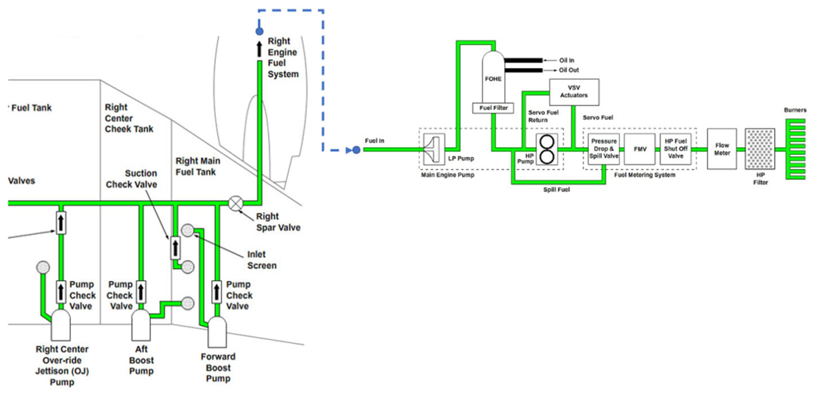
Figure 2.
Test Rig with components as indicated.
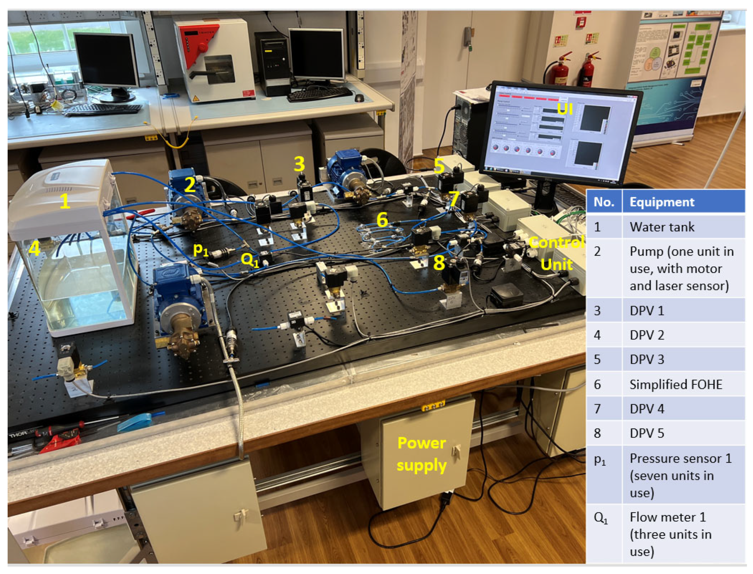
Figure 3.
Schematic of test rig, with components from Figure 2 cross-referenced.
Figure 3.
Schematic of test rig, with components from Figure 2 cross-referenced.
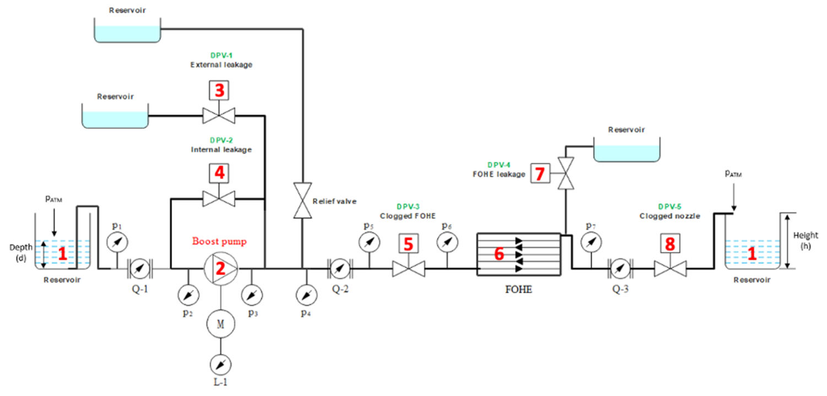
Figure 4.
Example of the unaveraged experimental data.
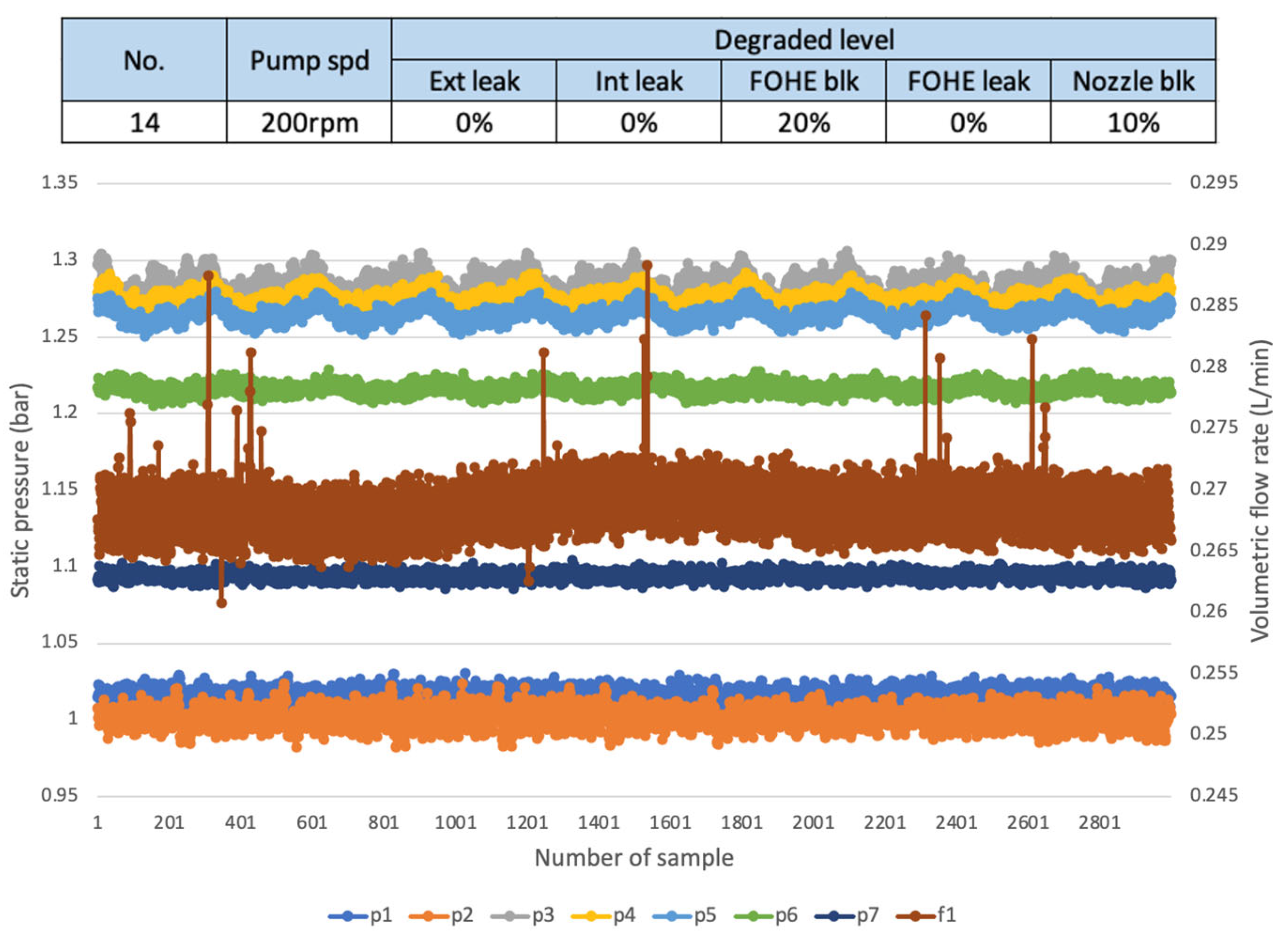
Figure 5.
Pressure ripple of pump suction and discharge.
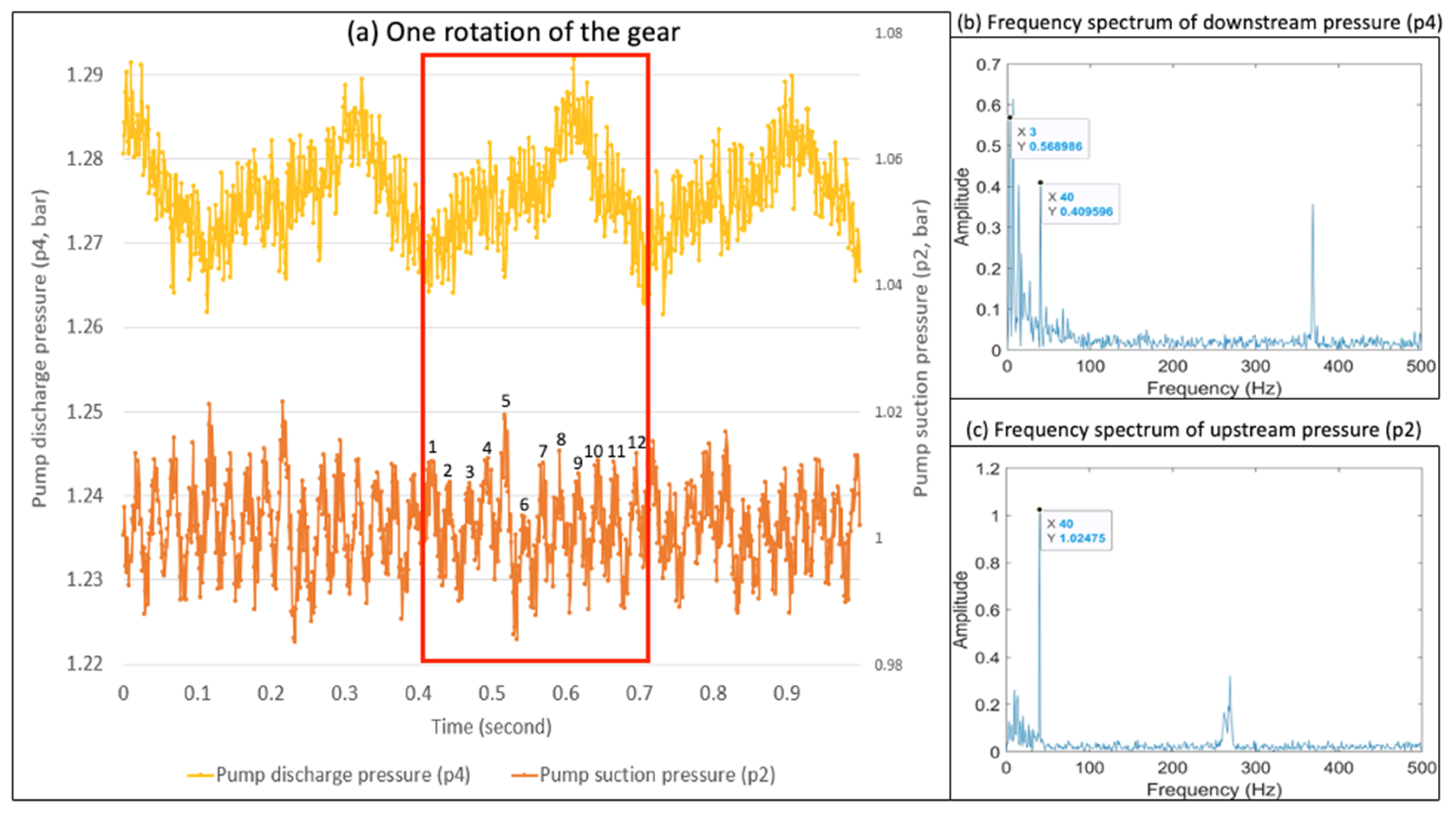
Figure 9.
Simulation validation results in healthy conditions.
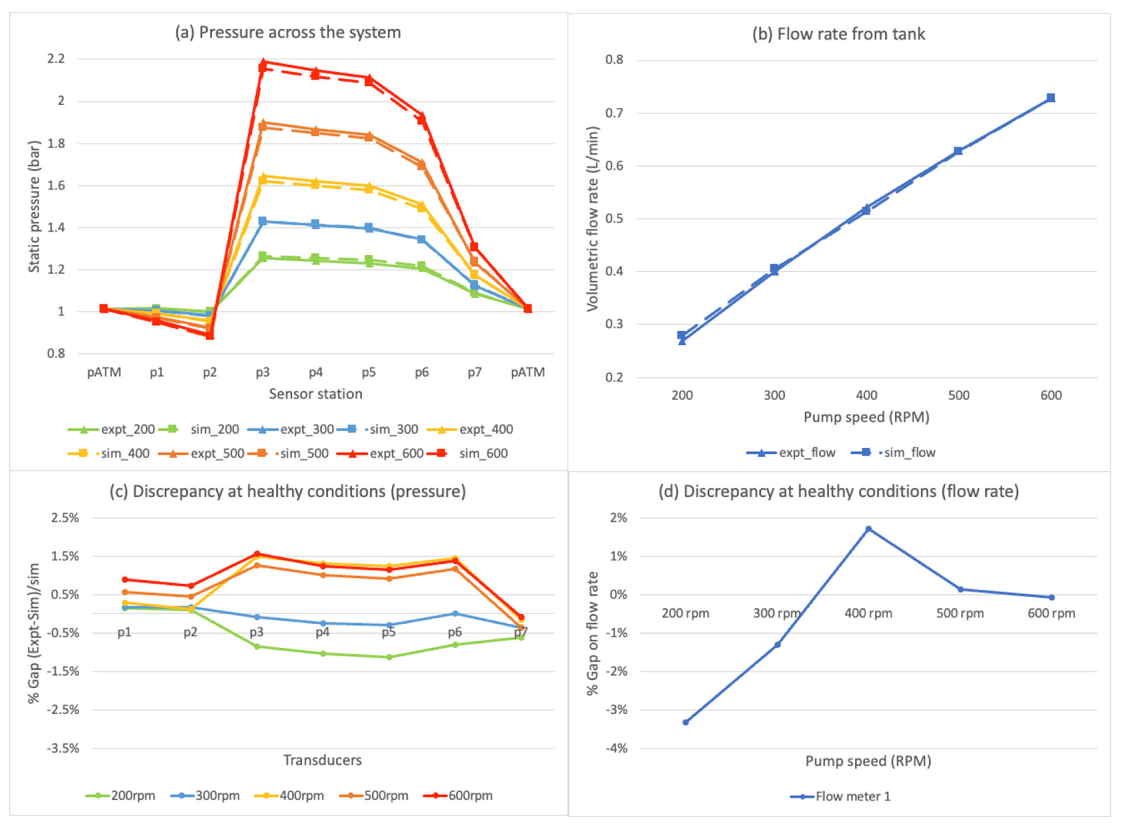
Figure 10.
Simulation validation results in faulty conditions.
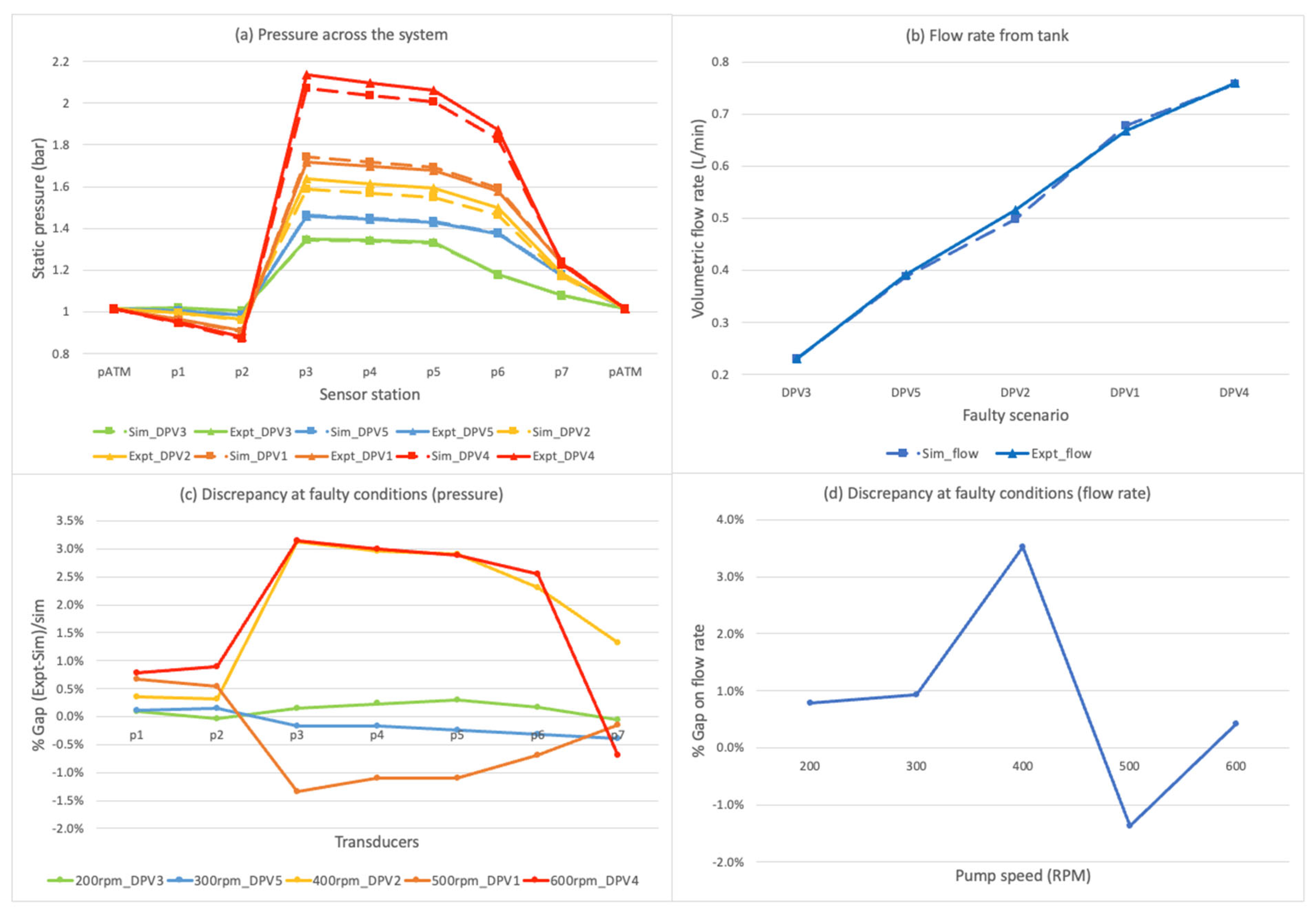
Figure 11.
Simulation validation results after matching the flow rate.
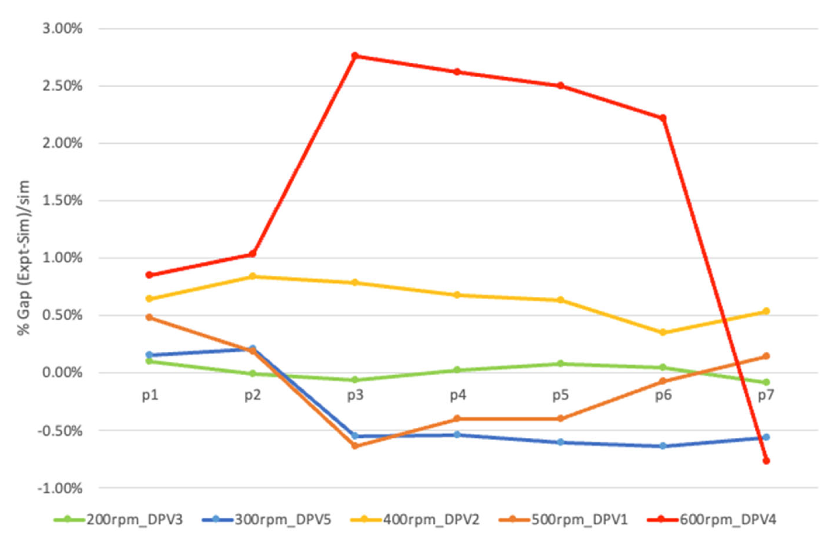
Figure 12.
Simulation results (single degradation scenarios, 400rpm).
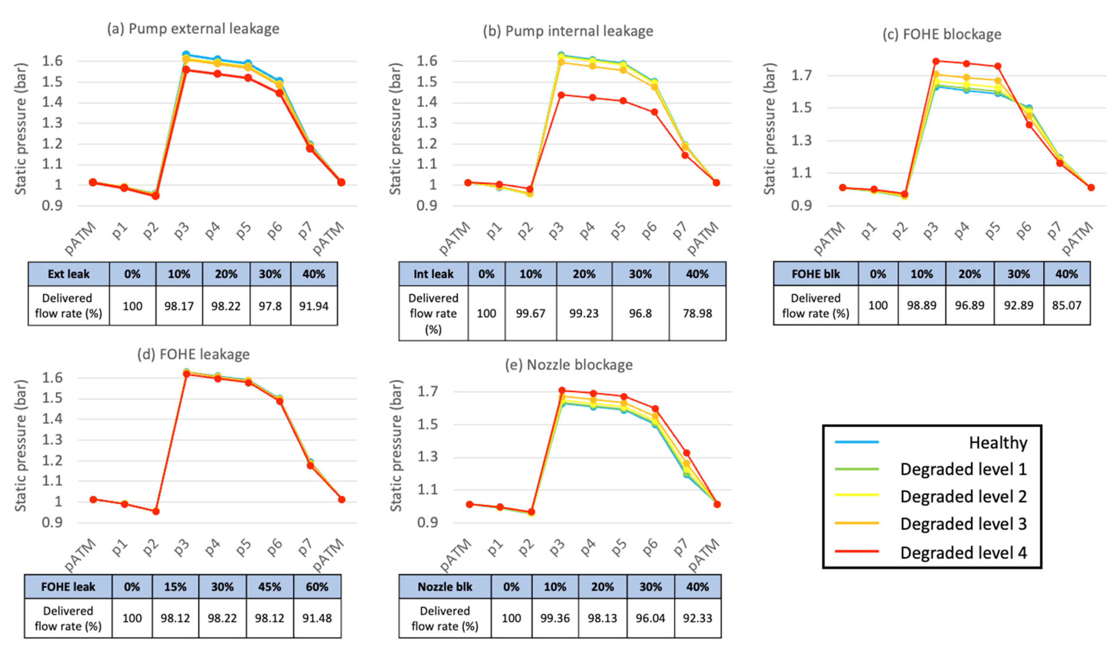
Figure 13.
Simulation results (multiple degradation scenarios, 400rpm).
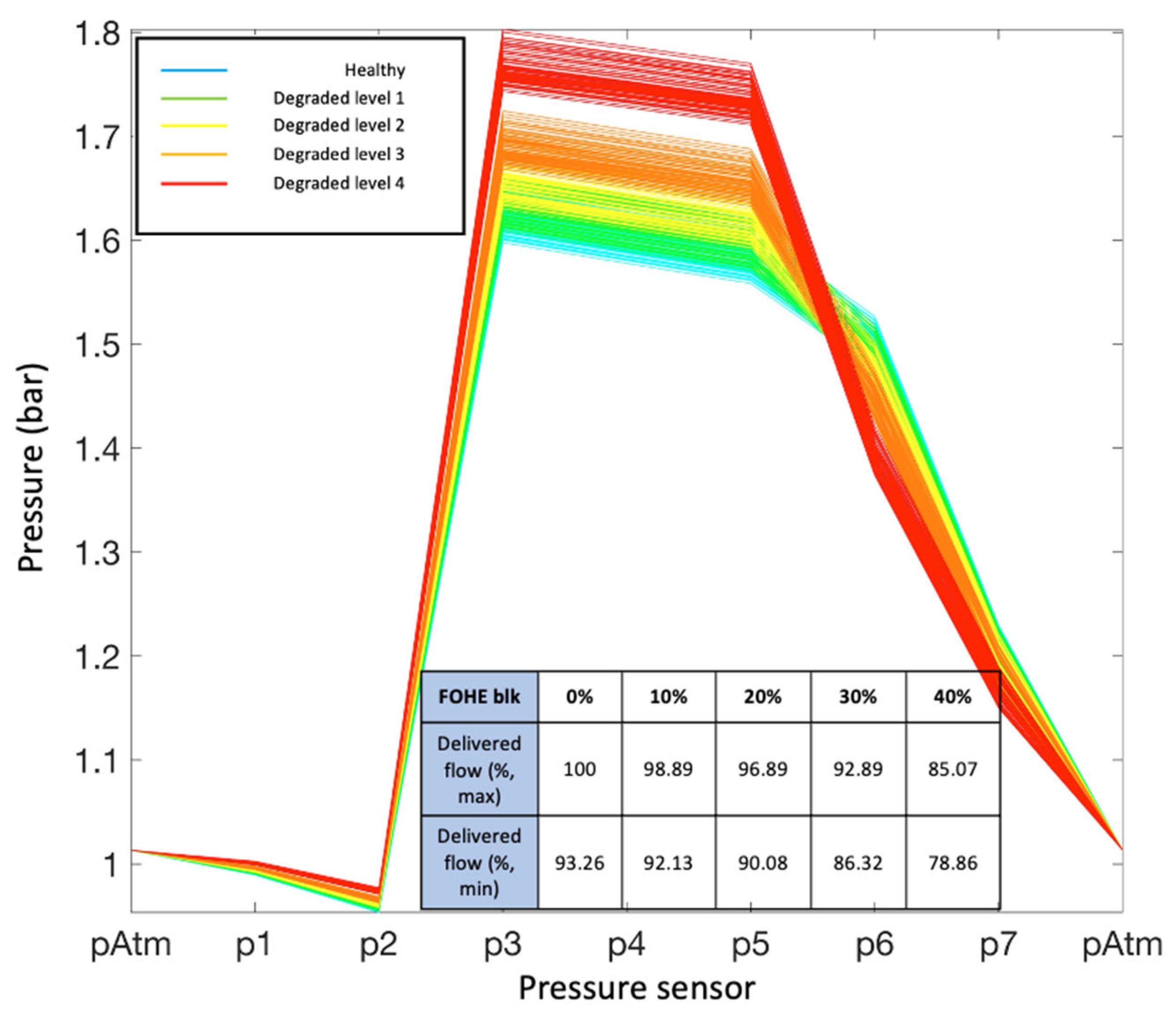
Figure 14.
The impact of each failure mode on the system’s behaviour.
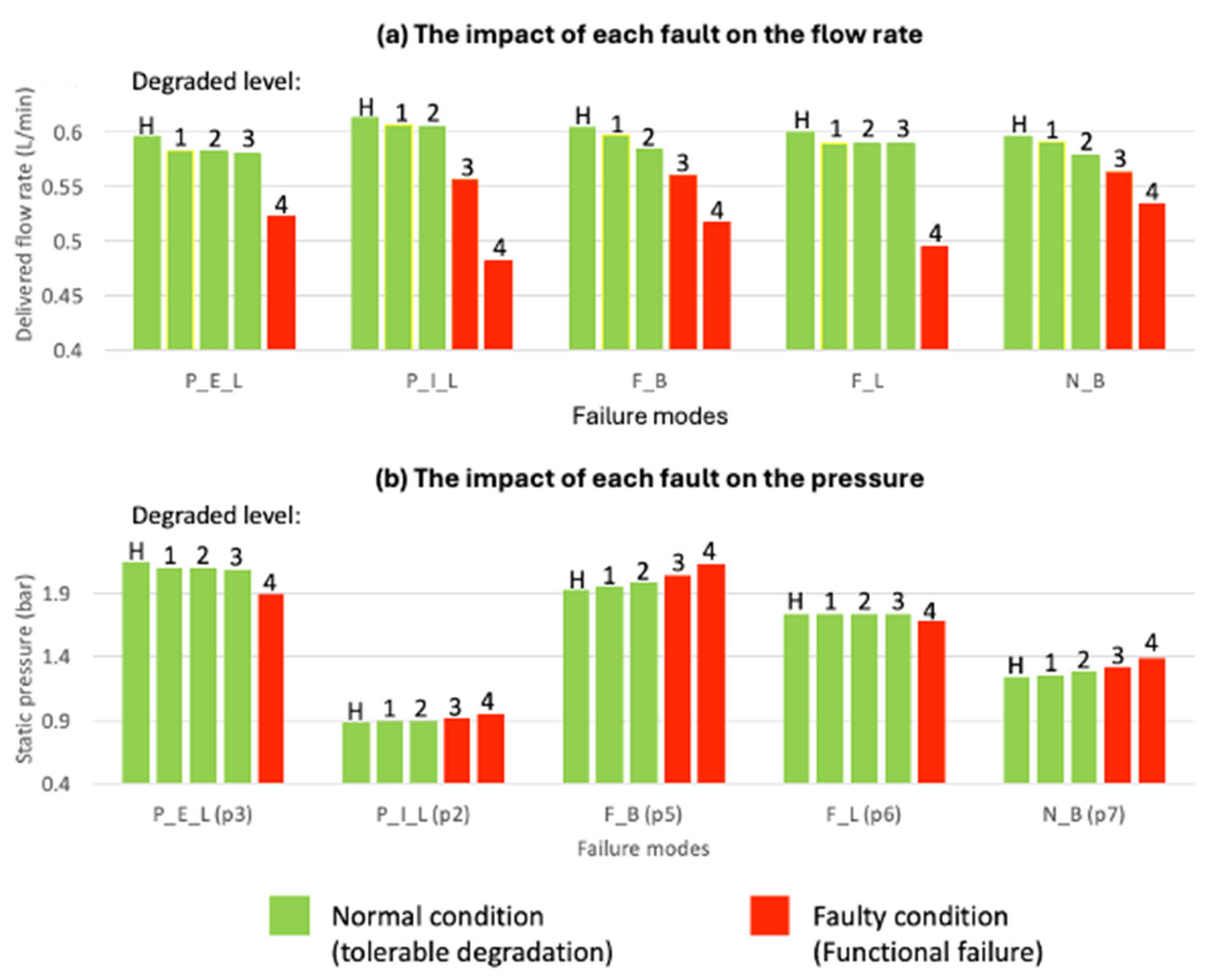
Figure 15.
Confusion matrix of Decision Tree in diagnosing pump external leakage.
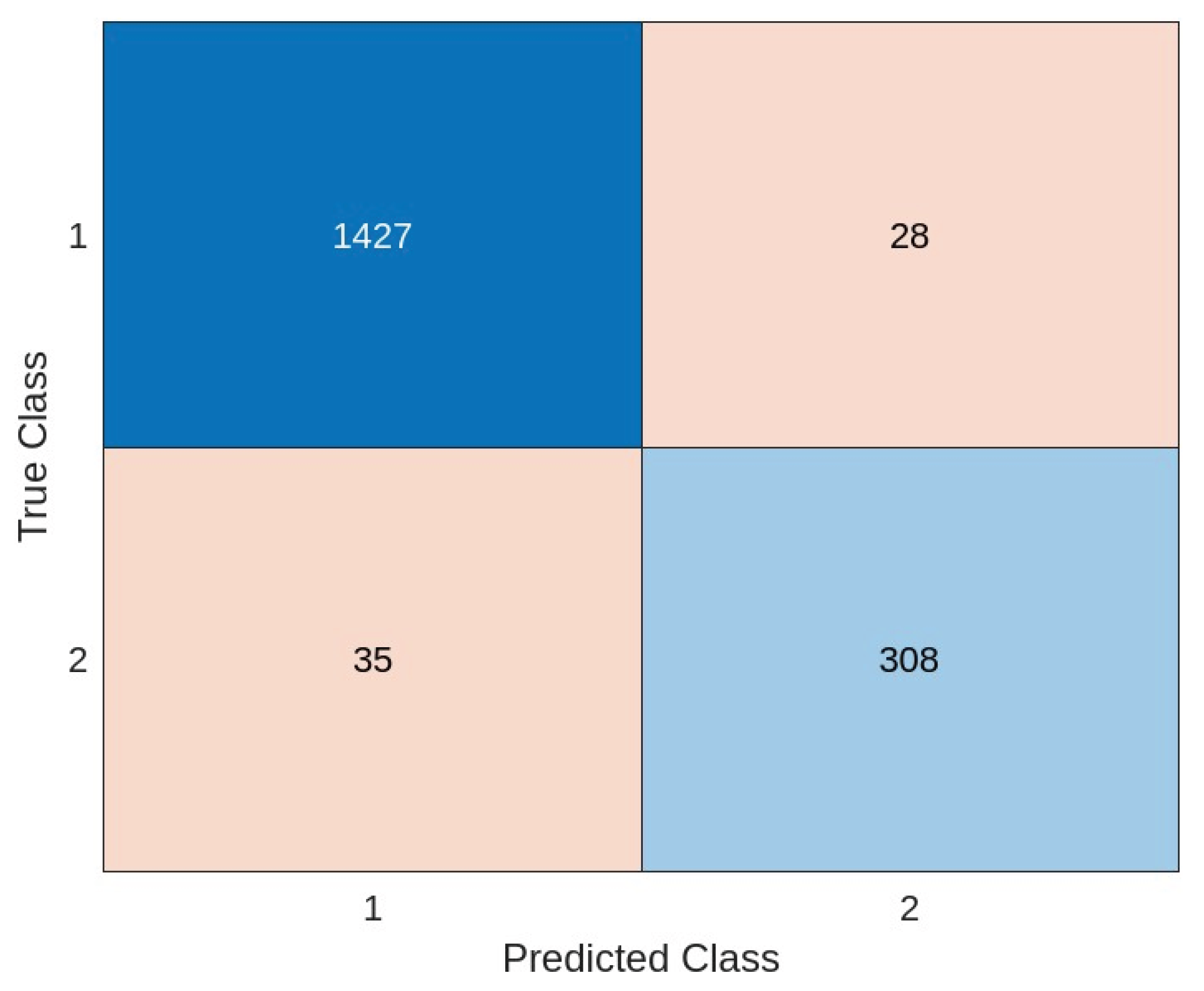

Table 1.
DPV configuration, fault types, and voltage mapping.
| ID in Figure 3 | Failure mode | DPV | Location | Nominal State | Severity definition | Command Voltage (V) | Equivalent opening | Affected path |
| 3 | Pump external leakage | DPV1 | Side branch | Normally closed (≈ 0 V) | Leakage severity s | V=10s | ≈100s % | Main → branch |
| 4 | Pump internal leakage | DPV2 | Side branch | Normally closed (≈ 0 V) | Leakage severity s | V=10s | ≈100s % | Main → branch |
| 5 | FOHE blockage | DPV3 | Main line | Fully open (≈ 10 V) | Closure fraction s | V=10(1-s) | ≈(1-s) 100% | Main-line throttling |
| 7 | FOHE leakage | DPV4 | Side branch | Normally closed (≈ 0 V) | Leakage severity s | V=10s | ≈100s % | Main → branch |
| 8 | Nozzle blockage | DPV5 | Main line | Fully open (≈ 10 V) | Closure fraction s | V=10(1-s) | ≈(1-s) 100% | Main-line throttling |
Table 2.
Working and health conditions of the test rig.
| Category | Name | Speed/Severity Range | Interval | Number of speeds/severities |
| Working conditions | Pump speed | 200~600 rpm | 100 rpm | 5 |
| Degradations | Pump external leakage | 0~40% | 10% | 5 |
| Pump internal leakage | 0~40% | 10% | 5 | |
| FOHE blockage | 0~40% | 10% | 5 | |
| FOHE leakage | 0~60% | 15% | 5 | |
| Nozzle blockage | 0~40% | 10% | 5 |
Table 3.
Unknowns and equations for solving the healthy condition.
| Boundary condition (atmospheric pressure plus water depth of the tank) | |||
| Nine unknowns | p0 | Nine Equations | Bernoulli equation |
| p1 | Pipeline 1 | ||
| p2 | Flowmeter 1 | ||
| p3 | Gear pump | ||
| p4 | Pipeline 2 | ||
| p5 | Flowmeter 2 | ||
| p6 | DPV 3 | ||
| p7 | FOHE | ||
| f1 | DPV 5 | ||
| Boundary condition (atmospheric pressure) | |||
Table 4.
Boundary setting for normal and abnormal conditions.
| Failure mode | Normal condition | Abnormal condition |
| Pump external leakage | 0%, 10%, 20%, 30% | 40% |
| Pump internal leakage | 0%, 10%, 20% | 30%, 40% |
| FOHE blockage | 0%, 10%, 20% | 30%, 40% |
| FOHE leakage | 0%, 15%, 30%, 45% | 60% |
| Nozzle blockage | 0%, 10%, 20% | 30%, 40% |
Table 5.
Configuration of selected ML algorithms.
| Algorithm | Configuration | Function in MATLAB |
| LR | Multinomial Logistic Regression | mnrfit |
| DT | MaxNumSplits = 1100, Prune = on | fitctree |
| SVM | KernelFunction = polynomial, PolynomialOrder = 4, Solver = ISDA | fitcecoc |
| ANN | Hidden layer size = 16, Activation function = sigmoid | fitcnet |
Table 6.
ML diagnostic results (F-1 scores).
| Pump external leakage | Pump internal leakage | FOHE blockage | FOHE leakage | Nozzle blockage | Efficiency | |
| LR | 0.9259 | 0.9152 | 1 | 0.9882 | 0.9921 | Slow |
| DT | 0.9072 | 0.897 | 0.981 | 0.927 | 0.9692 | Fast |
| SVM | 0.9034 | 0.9054 | 1 | 0.9324 | 0.9894 | Extremely slow |
| ANN | 0.9622 | 0.9417 | 1 | 0.9882 | 0.9961 | Fast |
Disclaimer/Publisher’s Note: The statements, opinions and data contained in all publications are solely those of the individual author(s) and contributor(s) and not of MDPI and/or the editor(s). MDPI and/or the editor(s) disclaim responsibility for any injury to people or property resulting from any ideas, methods, instructions or products referred to in the content. |
© 2026 by the authors. Licensee MDPI, Basel, Switzerland. This article is an open access article distributed under the terms and conditions of the Creative Commons Attribution (CC BY) license (http://creativecommons.org/licenses/by/4.0/).
Copyright: This open access article is published under a Creative Commons CC BY 4.0 license, which permit the free download, distribution, and reuse, provided that the author and preprint are cited in any reuse.


