
Submitted:
20 January 2026
Posted:
22 January 2026
You are already at the latest version
Abstract
We show that the GBFA method of Elgindy (2025), originally developed for 0 < α < 1, extends to all α > 0 without altering its algorithmic structure. Elgindy's transformation τ = t(1 − y1/α) remains valid for all α > 0 and preserves the numerical framework, ensuring that interpolation, quadrature, and error analysis carry over unchanged. For α > 1, the mapping induces only Hölder regularity at y = 0, which a ects quadrature accuracy. We quantify this e ect and show that the interpolation error retains its original convergence properties. To restore higher-order endpoint smoothness, we introduce a ϕ(α)-generalized transformation that enforces Cr regularity for any prescribed r ≥ 0, accelerating quadrature convergence while preserving the GBFA structure. Numerical experiments con rm high accuracy and robustness across all α > 0, demonstrating that the uni ed GBFA formulation provides an e cient, non-adaptive, xed-node approach for arbitrary-order RLFIs.
Keywords:
endpoint regularity
; fractional calculus
; fractional integration matrix
; Gegenbauer polynomials
; pseudospectral methods
; Riemann Liouville integral
; variable transformation
MSC: 26A33; 41A10; 41A25; 41A55; 42C05; 65D30
1. Introduction
Fractional calculus provides a powerful framework for modeling systems exhibiting memory, nonlocal interactions, and power-law dynamics [1,2]. Central to this theory is the RLFI of order , defined by
While fractional orders in have been extensively studied due to their prevalence in physical applications [42,43,44], emerging problems in applied electromagnetics [45], structural dynamics [46], intelligent infrastructure, electrical engineering, nonlinear dynamics, biomechanics, control systems, thermal and fluid sciences, and biomedical signal analysis increasingly require integration orders beyond this interval [47,48].
1.1. Challenges in Arbitrary-Order RLFI Computation
Despite its closed-form definition (1), the RLFI rarely admits an analytic expression for general f and arbitrary . Even for smooth or elementary f, the nonlocal kernel couples all past values of f, defying symbolic integration except in special cases (e.g., monomials or exponentials with integer ). Moreover, for non-integer , the kernel belongs only to , which precludes the use of classical higher-order Newton–Cotes or Gauss rules without transformation. In practical modeling–such as anomalous transport, viscoelasticity, and control–where f is often given numerically or as part of a coupled system, fast, stable, and repeated evaluation of becomes essential.
1.2. Overview of Existing Numerical Approaches
This need has spurred decades of research into numerical quadrature methods. Foundational work in polynomial-based and operational matrix methods for fractional calculus includes early contributions from orthogonal polynomial systems [52] as well as more recent extensions and refinements [50,51,54]. More recent developments include operational matrices using Charlier polynomials [24], fractional-order Chelyshkov functions [41,49], and SG-based GBFA schemes [4] that exhibit super-exponential convergence for —a result we later extend and refine in Section A.3, showing that full super-convergence of the classical GBFA formulation (including the quadrature component) occurs precisely when . Concurrently, spline interpolation schemes (linear to quintic) offered flexible local approximations with rigorous error estimates [25,26,53]. Composite and trapezoidal-type quadrature rules for fractional integrals, frequently combined with Romberg extrapolation, have been developed and analyzed in recent years [27,28]. In parallel, a variety of projection and operational matrix techniques–employing block-pulse functions, hybrid polynomial systems, and Galerkin formulations–have been developed over the past decade to improve computational efficiency [30,31,32,33,34,41]. Advanced quadrature techniques for weakly singular fractional integrals continue to be an active research area. These include variable transformations such as the sigmoidal Sidi–Laurie maps [56,57], Sinc-based collocation [37,38,39], and modern adaptations in Sobolev settings [35,36], all aimed at improving convergence by regularizing endpoint behavior. Spectral and wavelet bases, such as Mittag-Leffler wavelets, have further enhanced adaptivity and accuracy [40,55].
1.3. Limitations of Current Methods
While these existing alternatives provide valuable tools for specific regimes of , they generally lack one or more of the following attributes essential for high-performance, repeated RLFI evaluation: (i) fixed-node, non-adaptive structure compatible with global solvers; (ii) precomputable integration matrices enabling low online cost; (iii) generally offers rapid (often spectral) convergence for smooth f across all ; and (iv) tunable endpoint regularity to control quadrature accuracy. The GBFA framework developed in this work–extending the earlier approach of Elgindy [4]–uniquely satisfies all four properties simultaneously, as demonstrated later in the paper.
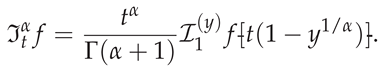
The GBFA method [4] employs the transformation
to obtain the exact identity
 Although the kernel of (1) is nonsingular on for , the composed integrand is only Hölder-continuous of order at , with all derivatives blowing up as (as we demonstrate later via Faà di Bruno’s formula). This loss of endpoint smoothness degrades Gauss-type quadrature convergence despite the original kernel being . Adaptive quadrature can compensate but is computationally expensive, non-reproducible across evaluations, and incompatible with fixed-grid solvers (e.g., collocation, operational matrices, time-stepping schemes). Hence, a unified, non-adaptive, highly accurate framework operating on fixed nodes, yielding precomputable FSGIMs, maintaining high algebraic, spectral, or even super-exponential convergence rates whenever the endpoint regularity permits, and integrating seamlessly into global approximation architectures remains compelling.
1.4. The GBFA Method and Its Original Scope
Within this landscape, Elgindy [4] introduced the GBFA method, which achieves super-exponential convergence for the RLFI when via SG interpolation and precomputable FSGIMs, while exhibiting algebraic convergence for other fractional orders ; cf. Section A.3. The method hinges on transformation (2), yielding identity (3), and exhibits: (i) super-exponential convergence for analytic f and ; (ii) precomputable FSGIMs; and (iii) tunable SG parameters , for optimal stability and accuracy. Although the original presentation restricted to , transformation (2) is mathematically valid as we show later in Section 3. This paper demonstrates that the entire GBFA framework–including SG interpolation, FSGIM construction, and error analysis–extends naturally to arbitrary without algorithmic modification. Additionally, we introduce and analyze a family of generalized -transformations that restore endpoint regularity for (for any ), thereby enabling high-order quadrature convergence across all . We further note that endpoint regularity is likewise attainable for whenever , as demonstrated later. This insight significantly broadens GBFA’s applicability to problems requiring or even integer-order repeated integration.
Existing alternatives for arbitrary-order RLFIs–such as adaptive quadrature [5], operational matrix techniques [6,7], and wavelet-based methods [8,9]–often trade accuracy for computational cost or implementation complexity. In contrast, the generalized GBFA preserves spectral accuracy, enables efficient FSGIM reuse, and, as shown herein, attains near machine-precision across with minimal parameter tuning.
1.5. Contributions of This Work
The main contributions of this work include:
- (i)
- A proof that the GBFA method of [4], originally developed for , requires no algorithmic modification to extend to arbitrary ;
- (ii)
- (iii)
- Numerical validation of excellent convergence rates and robust performance over a wide range of ;
- (iv)
- Introduction of a novel -generalized transformation for that enforces tunable endpoint regularity (for any prescribed ) in the transformed integrand, dramatically accelerating quadrature convergence and enabling near machine-precision accuracy with modest quadrature orders through appropriate choice of r and spectral parameters ; moreover, we show that endpoint regularity is likewise attainable for whenever , as demonstrated later.
- (v)
- Provision of a unified framework which delivers an exact algebraic substitution that precisely cancels the kernel for (classical case) while restoring controllable endpoint smoothness for (generalized case), and likewise for whenever ; this is distinct from approximate sigmoidal regularization techniques such as Sidi–Laurie transformations, which are primarily designed for weakly singular kernels when .
- (vi)
- A refined error analysis that establishes a complete convergence hierarchy for the ITE across all smoothness classes of f (globally analytic, Gevrey-regular with index , general , and finitely smooth ), clarifying the precise regularity conditions required for super-exponential, log-stretched-exponential, qualitative, or algebraic decay rates—extending and sharpening the bounds in [4], which focused primarily on analytic data.
- (vii)
- A sharp characterization of the endpoint regularity of the transformed integrand under Elgindy’s classical map, establishing that full super-exponential convergence of the GBFA method (including exact quadrature for polynomial data) occurs iff ; otherwise, the integrand belongs only to a Hölder space with and , limiting quadrature to algebraic asymptotic rates. In particular, for with , one may still enforce an error of order for any . Crucially, we clarify via Remark A9 that for real-analytic f, the pre-asymptotic quadrature error often decays dramatically faster than this worst-case rate due to exponentially decaying coefficients in the fractional power series expansion of the transformed integrand, reconciling observed near-exponential convergence in practical computations even when .
1.6. Organization of the Paper
The remainder of the paper is organized as follows: Section 2 reviews the GBFA framework of [4]. Section 3 proves this framework is valid , analyzes endpoint regularity, and presents convergence results for analytic, Gevrey, , and data, along with quadrature error and -dependence. Section 4 introduces the -generalized transformation, and constructs weighted FSGIMs. Section 5 analyzes complexity. Section 6 derives the smoothness condition. Section 7 validates both transformations for , compares GBFA against some methods and solvers available in the literature. Section 8 summarizes implications, guidelines, trade-offs, and future directions.
2. Background: GBFA Method
This section briefly summarizes the GBFA method as presented in [4], highlighting the components that naturally generalize to arbitrary .
2.1. SG Polynomials, the RLFI Transformation, and FSGIMs
As detailed in [4, Section 2], the SG polynomials , defined for and , form an orthogonal basis on with respect to the weight function . For and SGG nodes , the GBFA interpolant is:
 where are the Lagrange basis polynomials in SG form. The core innovation in [4] is Elgindy’s transformation (2), which, for , yields (3). The GBFA approximation then becomes:
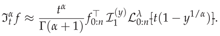
The approximation formula (5) shows that the RLFI reduces, after the transformation (2), to evaluating integrals of the form
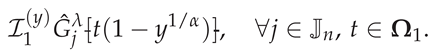 We refer to (6) as the SG–transformed integrals. They arise naturally from substituting the SG interpolant of f into the transformed RLFI and represent the contribution of each SG basis function to the fractional integral.
Because the mapping is a -diffeomorphism on the open interval for all , the integrands in (6) are smooth functions of y on , even when the original RLFI kernel is weakly singular for . This interior regularity supports high-order SG quadrature convergence. However, for , the mapping is only Hölder-continuous of order at the endpoint , with all derivatives blowing up as (as shown later in Section 3.6). This endpoint behavior reduces the global regularity of the transformed integrand on , affecting the quadrature error component but not the interpolation error (which depends only on the smoothness of f in the original variable t).
In practice, the integrals (6) are approximated using high-order Gauss quadratures such as the -GBFA quadrature rule [4]. This introduces a quadrature truncation error that we will analyze later in Section 3.5 for arbitrary . The explicit definition (6) is therefore essential for understanding both the construction of the FSGIMs and the total error structure of the GBFA method.
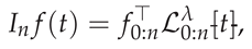
As developed in [4, Section 3], the th-order FSGIM enables efficient computation:
for evaluation points . These matrices are precomputable and depend only on , n, , and quadrature parameters; see [4, Eqs. (18) and (20)].
Motivated by the structural properties reviewed above, we now turn to one of the central theoretical contributions of this work.
3. Generalization to Arbitrary Fractional Orders
With the essential machinery now in place, we demonstrate in this section how the GBFA framework naturally extends to arbitrary without modification.
3.1. Mathematical Validity of Elgindy’s Transformation
The transformation (2) requires careful examination of the exponent . For , the mapping (2) is bijective on with Jacobian (A46) (see A.2). Substituting into the RLFI definition yields:
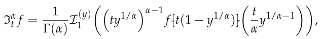 which directly institutes (3). Notice here the precise cancellation of the exponents of y: the term arising from the kernel is perfectly neutralized by the term appearing in the Jacobian . This identity holds for all ; thus, the core GBFA framework—including the approximation formula (5), the FSGIM construction from [4, Section 2], and the evaluation form (7)—extends directly to arbitrary positive orders without modification. Since the transformation (2) is exact for all , the algorithm for generating requires no -dependent changes. However, for , the endpoint regularity of the transformed integrand is reduced (becoming only Hölder-continuous of order at ), which affects the quadrature truncation error component but leaves the interpolation error convergence rate intact as we prove later in Section 3.6.
With the transformation rigorously justified, we can now analyze how the error structure behaves under arbitrary fractional orders.
3.2. Error Analysis
The error analysis developed in [4, Section 4] carries over to the present framework without any change in the proof structure or asymptotic rates; only the constants in the bounds acquire an implicit dependence on through the composed integrand . The corresponding convergence results are given below in Theorems 1–5, covering analytic, Gevrey-regular, general -smooth functions, and finitely smooth data with algebraic convergence rates. In particular, Theorems 1 and 2 quantify super-exponential and log-stretched-exponential decay for analytic and Gevrey-regular inputs, Theorems 3 and 4 ensure qualitative convergence for data, and Theorem 5 establishes algebraic convergence of order for functions in .
Theorem 1
(Super-Exponential Convergence for Globally Analytic f). Let and . Suppose that f is real-analytic on and that there exist constants such that
Let be approximated via the GBFA method using SG interpolation of degree n. Then such that the ITE admits the exact representation
 where is given by [4, Eq. (24)]. Moreover, the GBFA approximation converges to at a super-exponential rate in n; more precisely, there exists a constant independent of n such that
Proof.
The exact error representation (10) follows directly from [4, Theorem 1], which remains valid for any since the transformation (2) is a -diffeomorphism between and ; see Corollary A2. To obtain an explicit asymptotic bound, we invoke the general estimate derived in [4, Theorem 2], which yields
where
and
with . By assumption (9), we have the growth bound
Substituting (14) into (12) gives
Collecting the n-dependent factors, we may rewrite (15) as
for some constant independent of n. Since is at most algebraic in n, there exists and such that
Thus,
and independent of n. As , the dominant term in the exponent is . Hence, there exists and such that
which implies
This proves that the GBFA error decays super-exponentially in n under the growth condition (9). □
The following theorem is tailored for smooth, but non-globally analytic function f; see, for example, [13] for a detailed discussion of Gevrey-regularity. By log-stretched-exponential convergence here we mean stretched-exponential with logarithmic enhancement; i.e., faster than stretched-exponential but slower than exponential.
Theorem 2
(Log-Stretched-Exponential Convergence for Gevrey Regular f). Let and . Suppose that f is -smooth on and that there exist constants and such that
Let be approximated via the GBFA method using SG interpolation of degree n. Then such that the ITE admits the exact representation (10). Moreover, there exists a constant independent of n such that
In particular, the GBFA approximation converges faster than any algebraic rate in n for Gevrey-regular f of order μ.
Proof.
As in Theorem 1, the exact error representation (10) follows from [4, Theorem 1] and the diffeomorphism property of the transformation (2). Consider again the general GBFA error estimate (12). Under the Gevrey growth condition (18), we have
Using Stirling’s approximation , we obtain
Substituting (20) and (21) into (12), and absorbing and the factor into a generic constant, we obtain n:
independent of n. Since grows at most algebraically in n, there exist and such that
Thus, from (22) we obtain
and independent of n. Writing the right-hand side of (23) in exponential form,
For , the coefficient is negative, hence the leading term is
which dominates the lower-order contributions and as . Therefore, there exist constants , , and such that
Since and , it follows that
, which proves (19). □
Theorem 3
(Qualitative Convergence for Higher-Order Gevrey-Regular f). Let and . Suppose that f is -smooth on and that there exist constants and such that
Let be approximated via the GBFA method using SG interpolation of degree n. Then the GBFA approximation converges pointwise to the exact RLFI, i.e.,
Moreover, the convergence is uniform in t on any compact subset .
Proof.
The Gevrey condition (24) with implies that . For such smooth functions, spectral interpolation at Gauss-type nodes yields uniform convergence. Specifically, for SG interpolation at the SGG nodes , there exists a sequence with such that
This follows from standard results in polynomial approximation theory; see, e.g., the convergence properties of interpolation in orthogonal polynomial bases at Gauss quadrature nodes [10,11,12,58].
Next, the RLFI defines a bounded linear operator on . For any ,
Applying this bound with and using (26), we obtain for every :
Consequently, for any fixed , since , we have the pointwise convergence (25).
For the uniform convergence on compact subsets, let be compact. Then , and we obtain
which establishes uniform convergence on K. □
Theorem 4
(Qualitative Convergence for Smooth Data). Let and . Suppose that and that, for each , denotes the SG interpolant of f at the SGG nodes as in (4). Assume that the SG interpolation operator satisfies
Let be approximated via the GBFA method using SG interpolation of degree n. Then (25) is satisfied, and the convergence is uniform in t on any compact subset .
Proof.
By assumption and (29) holds, i.e., the SG interpolants at the SGG nodes converge uniformly to f on . This is precisely the interpolation property used in the proof of Theorem 3, where the Gevrey condition (24) was invoked only to guarantee smoothness and the uniform convergence of SG interpolation. The remaining step in the proof of Theorem 3 relies on two ingredients: (i) the bounded linearity of the RLFI on , and (ii) the uniform convergence of to f in . These ingredients are entirely independent of the Gevrey growth condition and require only (29). Consequently, the same argument shows that (25) holds true for each fixed , and that the convergence is uniform in t on any compact subset . This establishes the proof. □
Remark 1
(Minimal Versus Structured Regularity). Theorem 4 identifies minimal smooth-data assumptions for qualitative convergence of the GBFA method–namely: (i) f is -smooth on , and (ii) the SG interpolants converge uniformly to f as in (29). In fact, the proof of convergence fundamentally relies only on the interpolation property (29) and the boundedness of the RLFI operator, and does not preclude convergence in weaker function spaces. By contrast, Theorem 3 concerns the more restrictive class of Gevrey-regular functions with index . Although this theorem also yields qualitative convergence, it plays a different conceptual role: it completes the Gevrey hierarchy established in Theorems 2–3 and shows that, as the Gevrey index crosses the threshold , the GBFA method transitions from quantitative (stretched-exponential) convergence to purely qualitative convergence. Thus, Theorem 3 serves to characterize the behavior of the GBFA method across the full spectrum of Gevrey regularity, whereas Theorem 4 isolates the weakest smooth-data conditions under which convergence still holds in this framework.
3.3. Dependence of the GBFA ITE on the Parameter
The dependence of the GBFA ITE on the SG parameter arises through several components of the general estimate (12). The dominant -dependence is contained in the constant , which, as shown in [4], is unimodal in , attaining its maximum near and then decaying exponentially as increases. This exponential decay is the primary mechanism governing the behavior of the error with respect to . In contrast, the remaining -dependent factors in (12), namely the algebraic term and, for , the auxiliary factor , contribute only algebraic growth or decay in n. For fixed n, these algebraic contributions are dominated by the exponential decay of , and therefore do not alter the qualitative trend that the GBFA ITE decreases as increases beyond .
For moderate fractional orders , this unimodal structure of explains why increasing improves the ITE. For larger , the dominant factor in (13) decays super-exponentially, suppressing the -dependence of all terms in (12). This accounts for the numerical observation in Section 7 that, for , the GBFA error becomes nearly invariant across all tested values of . Although the analysis in [4] focused on , the structure of the -dependent terms in (12) remains unchanged for all , and the qualitative behavior of the ITE with respect to therefore extends naturally to arbitrary fractional orders.
Figure 1 extends the numerical study of [4, Fig. 3] from the classical regime to fractional orders . The results exhibit the same qualitative structure observed previously: for moderate values of (e.g., ), the GBFA error retains a clear dependence on the SG parameter , with smaller errors obtained for increasing , in agreement with the unimodal behavior of described earlier in this section. As increases further, the dominant factor in the constant decays super-exponentially, effectively suppressing the -dependence of the entire bound (12). This explains the near-coincidence of all curves for increasing values in the classical transformation, where the total GBFA error is dominated by the quadrature component. In this regime, the super-exponential decay of the factor in suppresses the underlying -dependence, so the method appears only weakly sensitive to . Thus, Figure 1 demonstrates that the parameter-sensitivity patterns reported in [4] for persist for , but gradually diminish as grows, in full agreement with the theoretical predictions.
Remark 2.
Although the theoretical bound (12) indicates that the dependence on λ should diminish as α increases, numerical experiments using the -generalized transformation introduced in Section 4 exhibit a more nuanced trend. For this generalized mapping, moderate values of λ (typically ) continue to deliver excellent accuracy for large α. In contrast, extreme values near the theoretical lower limit show noticeably degraded performance as α grows, effectively widening the practical λ-sensitivity range. These observations suggest that, in applications of the generalized transformation, λ should be selected from to avoid the blow-up region near , while should be fixed at to fully exploit the endpoint regularization, as demonstrated in Section 7.3.
3.4. Finite Smoothness Case
The previous results focused on globally analytic functions, Gevrey-regular data, and -smooth functions. In many practical applications, however, the input f may possess only finite smoothness, say for some finite . In this case, one expects algebraic—rather than (super-)exponential—convergence, in line with classical results from spectral and pseudospectral approximation theory; see, for example, [11]. The following theorem formalizes this behavior for the GBFA approximation of the RLFI.
Theorem 5
(Algebraic convergence for data). Let and . Suppose that for some integer , and that its kth derivative satisfies
for some constant . For each , let denote the SG interpolant of f at the SGG nodes as in (4). Then there exist constants , independent of n, such that
and the GBFA approximation of the RLFI satisfies the algebraic error bound
In particular, the GBFA approximation of converges to the exact RLFI at an algebraic rate as for every fixed .
Proof.
By assumption with bounded kth derivative (30). For polynomial approximation on with respect to an orthogonal basis associated with a Jacobi-type weight (in particular, SG polynomials), classical Jackson-type estimates and interpolation results imply that there exists a constant , independent of n, such that the SG interpolation error at the SGG nodes satisfies the algebraic bound (31) for every fixed [14,15].
Remark 3
(Convergence Hierarchy for Smooth Functions). The GBFA method exhibits a classical smoothness-dependent convergence hierarchy in terms of its ITE:
- Globally analytic f (): Super-exponential convergence as shown by Theorem 1.
- Gevrey-regular f with : Log-stretched-exponential convergence as shown by Theorem 2. This naturally interpolates between algebraic and super exponential rates.
- Gevrey-regular f with (and general data): Qualitative convergence guaranteed but no explicit rate from current analysis (Theorems 3 and 4). The restriction in Theorem 2 is essential because for , the leading term in the error exponent becomes non-negative, requiring different analysis techniques.
- Finite smoothness : Algebraic convergence as shown by Theorem 5.
This hierarchy demonstrates that the GBFA method preserves the classical spectral property: convergence accelerates with increased smoothness of f, from algebraic for finitely differentiable functions to super-exponential for analytic functions. The RLFI operator does not alter this fundamental behavior but merely introduces a bounded scaling factor dependent on α and t.
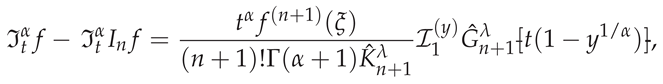
3.5. Quadrature Truncation Error for GBFA-Based RLFI
In the GBFA framework for , the SG–transformed integrals (6) appearing in the RLFI approximation are evaluated numerically using the –GBFA quadrature; cf. the SGIRV construction in [16, Algorithms 6–7]. This numerical step introduces a quadrature truncation error that combines with the interpolation error to determine the total accuracy of the method. The quadrature truncation error for SG–based RLFI integrands is rigorously characterized in [4, Theorems 3–4]. These results provide a closed-form expression for the quadrature truncation error in terms of the th SG derivative of the composed integrand, and sharp asymptotic bounds describing its decay with respect to , including the regimes and . In particular, [4, Theorem 3] gives the exact quadrature error representation for each SG mode j, while [4, Theorem 4] establishes its asymptotic decay rate and the influence of the quadrature index . Finally, the quadrature error produced by the –GBFA rule combines with the SG interpolation error analyzed in Theorems 1–5 to yield the total truncation error of the GBFA method. A complete asymptotic bound for this combined error is already established in [4, Theorem 5]. For analytic functions (Theorem 1), the regularity assumptions required by [4, Theorem 5] are fully satisfied, so the total GBFA error inherits the super-exponential decay in n coming from the ITE together with the fast decay in associated with the –GBFA quadrature. In particular, as shown in [4, Theorem 4], the quadrature error exhibits a two-regime structure: it vanishes identically whenever , and for its dominant terms decay exponentially in (up to algebraic prefactors depending only on and ) under the smallness conditions on and specified in [4, Eqs. (41) and (43)], where . Consequently, for analytic f, the total truncation error of the GBFA method is typically dominated by the interpolation component and therefore decays super-exponentially in n, while the quadrature component either vanishes or becomes negligible for sufficiently large in the admissible parameter regime. Thus, the overall accuracy of the GBFA method is governed jointly by the smoothness class of f and the chosen interpolation and quadrature parameters: the interpolation component decays at the rate dictated by the regularity of f, whereas the quadrature component is either zero or decays at least exponentially in when the transformed integrand is sufficiently smooth (e.g., when ); otherwise, it exhibits algebraic convergence due to limited endpoint regularity.
Remark 4
(On the Smoothness Assumptions in the GBFA Error Analysis [4]). The truncation–error analysis in the GBFA work [4] (Theorems 1–5 therein) is carried out under the single assumption that , since the Lagrange interpolation remainder formula requires the existence and boundedness of . No distinction is made between analytic, Gevrey-regular, , or finitely smooth data; all bounds are expressed in terms of the quantity together with asymptotic properties of SG polynomials and Gamma function estimates.
It is important to note that the super-exponential decay in [4] is generally valid for when the derivatives of f satisfy an analytic-type growth condition of the form , which ensures that does not dominate the polynomial–asymptotic factors. For general functions, however, the derivatives may grow at rates comparable to (Gevrey), (higher-order Gevrey), or even faster, in which case the factor may prevent super-exponential decay.
The present paper refines the convergence analysis by establishing a complete hierarchy of smoothness classes–globally analytic, Gevrey-regular (), general , and finitely smooth –and derives the corresponding decay rates for the ITE in each case. This clarifies that super-exponential convergence of the total GBFA error is achieved only when two conditions hold simultaneously: (i) f is globally analytic (ensuring super-exponential ITE decay per Theorem 1), and (ii) , under which the classical transformation (2) renders the SG–transformed integrands (6) real-analytic (indeed, polynomial if f is polynomial). In this special regime, the –GBFA quadrature is exact for , eliminating the quadrature truncation error entirely and yielding full super-convergence of the total error–even for functions whose derivatives grow rapidly–as confirmed in Theorem A10.
3.6. Endpoint Regularity of the Transformed Integrand for
The GBFA method relies on the transformation (2), which eliminates the algebraic kernel factor in the RLFI. After applying (2), the RLFI integrand becomes
which appears inside the SG–transformed integrals (6). Even when f is assumed smooth on , the mapping is not at when . This subsection clarifies the precise regularity of g near and its implications for the GBFA error structure.
Lemma 1
(Regularity of for ). Let and set . Then:
- (i)
- is continuous on and analytic on .
- (ii)
- For every integer ,
- (iii)
- Since , all derivatives blow up at :
In particular, since , the map is Hölder-continuous of order β on , but its derivatives blow up at ; hence it belongs to but not to .
Theorem 6
(Regularity of the Transformed Integrand g for ). Let and define g by (33). Assume that . Then and real-analytic on .
Proof.
Let and set . Define the inner map
By Lemma 1, the function is continuous on and analytic on , with all derivatives blowing up at . Since , the composition is analytic on by the chain rule for analytic functions.
For the global regularity on , we analyze the derivatives of g at . By Faá di Bruno’s formula for the mth derivative of a composition [17], we have
where are the (partial) Bell polynomials in the derivatives of . Each term in this sum is a finite linear combination of monomials of the form
where the nonnegative integers satisfy
Using Lemma 1, each derivative behaves like
so the product scales as
for some constant depending only on and the multi-index . Thus, every Faà di Bruno term in is asymptotically of the form
To identify the most singular contribution, we note that for fixed m the exponent is strictly increasing in k because . Hence the smallest exponent (i.e., the most negative, and therefore the most singular) corresponds to the smallest possible k. Since , the dominant contribution arises from the terms with . For such terms we have
and the corresponding part of behaves like
In particular, if , then as , and the factor controls the singular behavior of near . For to remain bounded as , we require , i.e., . Since for every , no integer satisfies . Thus, unless , the dominant contribution (34) already becomes singular for , and higher derivatives exhibit even stronger divergence. If , the leading singular term vanishes, but similar divergences reappear in higher-order contributions unless f possesses sufficiently high-order zeros at t. This establishes the proof. □
Remark 5
(Effect on GBFA Error: Quadrature vs. Interpolation). The finite endpoint regularity described in Theorem 6 affects only the quadrature error associated with approximating the SG–transformed integrals (6) using the –GBFA quadrature rule. For , the composed integrand g is merely Hölder-continuous of order at , which directly reduces the global regularity of g on and significantly slows the convergence of the quadrature truncation error component compared to the case. This quadrature error dominates the total error for analytic f, limiting the overall convergence rate of the GBFA method and causing it to degrade as α increases (with larger α yielding slower quadrature convergence for fixed ). Importantly, the ITE in the original variable t remains unaffected and retains super-exponential decay in n. Thus, while the interpolation component preserves the full spectral rate dictated by the smoothness of f, the total GBFA accuracy for is governed primarily by the typically algebraic quadrature decay, requiring substantially larger to maintain high accuracy as α grows, as confirmed numerically in Section 7.
3.7. Endpoint Regularity of the Transformed Integrand for ,
We now analyze the SG–transformed integrand g defined in (33) for the regime . In contrast to the case of Subsection 3.6, the inner map exhibits higher endpoint smoothness when , and this improved regularity propagates to g.
Lemma 2
(Regularity of for , ). Let and with . Then:
- (i)
- is continuous on and analytic on .
- (ii)
- For every integer , the derivative formula from Lemma 1(ii) applies with , and the exponent determines the endpoint behavior.
- (iii)
- remains finite at iff , and diverges for all .
Hence and .
Theorem 7
(Regularity of the Transformed Integrand g for , ). Let and define g by (33). Assume . Then:
and g is analytic on .
Proof.
Let . The derivatives of are given by the same expressions used in the proof of Theorem 6, with the scaling inherited from Lemma 1. Applying Faà di Bruno’s formula [17] exactly as in Subsection 3.6 yields
since the dominant contribution again corresponds to in the Bell-polynomial expansion. Because , the quantity is nonnegative precisely when , and negative for . Thus is finite for and diverges otherwise, unless f has sufficiently high-order zeros at t. This proves the stated regularity. □
Remark 6
(Effect on GBFA Error for , ). The endpoint smoothness in Theorem 7 improves the SG–quadrature behavior relative to the case. Since g now possesses regularity at , the –GBFA quadrature applied to (6) achieves a higher-order algebraic decay rate than that described in Remark 5. The ITE in t remains unchanged and retains super-exponential decay in n. Consequently, for , the total GBFA error is governed by a faster quadrature convergence that improves as α decreases.
4. Restoring Endpoint Regularity via a Generalized Transformation
For , the transformation (2) remains mathematically valid; however, as shown in Section 3.6, the mapping is only Hölder-continuous of order at , and all derivatives blow up as . This loss of endpoint regularity affects only the quadrature truncation error component of the GBFA method. For with , the same mapping exhibits a complementary limitation: although is differentiable at , its higher-order derivatives fail to exist due to the noninteger exponent. Consequently, , the transformation (2) imposes endpoint smoothness restrictions that may reduce the global regularity of the transformed integrand. To improve the global smoothness of the transformed integrand for such values of , we introduce the generalized mapping
The mapping (35) is a -diffeomorphism on for every (see A.4), with
Substituting (35) into the RLFI definition (1) yields the exact identity
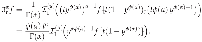 Thus, for , the RLFI reduces to evaluating weighted SG-transformed integrals of the form
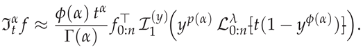
 in place of the unweighted integrals (6). The GBFA approximation corresponding to (36) becomes
4.1. Weighted FSGIM Construction
5. Computational Complexity of the Weighted FSGIM
We analyze the computational complexity of the weighted FSGIM defined row-wise by (40). Let denote the SG interpolation degree, the GBFA quadrature order, and the number of evaluation points, respectively. As in [4], the computation of the SG polynomials using the three-term recurrence relation requires operations per degree. Since polynomial evaluations are required for all degrees up to n, this stage contributes operations per entry of .
For a fixed evaluation point , the construction of  requires evaluating the SG-based expressions at the transformed quadrature nodes, which incurs an additional flops. The vector is computed in flops, and forming the outer product requires multiplications. The Hadamard product with introduces another multiplications. Applying to collapse the rows into one row requires dot products of length , i.e., flops, and the scalar factor adds flops.
requires evaluating the SG-based expressions at the transformed quadrature nodes, which incurs an additional flops. The vector is computed in flops, and forming the outer product requires multiplications. The Hadamard product with introduces another multiplications. Applying to collapse the rows into one row requires dot products of length , i.e., flops, and the scalar factor adds flops.Collecting the dominant terms, the overall per-row cost of constructing the weighted FSGIM is
with constant factors at most a small multiple of the classical case. Therefore, constructing for all entries of requires flops. Once is available, applying the FSGIM to is a dense matrix–vector multiplication costing flops in both the classical and weighted cases.
6. Endpoint Regularity and the Choice of
The transformed integrand in (37) is
For analytic f, g is analytic on , but its smoothness at depends on the competition between the vanishing weight and the singular derivatives of as . A Faá di Bruno–type exponent analysis shows that a sufficient condition for is (A48); see Section A.5. This condition provides a practical design rule: choosing according to (A48) guarantees that the transformed integrand is at least at . Since Gauss–type quadrature for functions converges algebraically at a rate , the choice of r directly controls the quadrature truncation error.
Remark 7
(Trade-offs in the Choice of ). The mapping (35) enables a tunable balance between endpoint smoothness and weight concentration:
- Choosing yields perfect kernel cancellation and recovers the original GBFA identity (3), but the transformed integrand is only Hölder-continuous at for .
- Choosing according to (A48) yields a integrand at , improving the quadrature convergence rate to by Theorem A12 and Corollary 1.
- Larger r increases smoothness but also increases the weight exponent , which may over-concentrate the integrand near ; cf. Figure 2. This concentration can degrade quadrature accuracy unless both and are appropriately chosen. Specifically, controls the node distribution, while must be sufficiently large to resolve the sharp peak near .
Although the generalized -framework and its associated smoothness condition (A48) were developed primarily for , the underlying results extend naturally to all . In particular, for with , one may enforce regularity via (A48), guaranteeing algebraic quadrature convergence . However, this approach is not recommended in practice. For , the classical transformation yields the exact, weight-free identity (3) and, for real-analytic f, induces a fractional power series expansion with exponentially decaying coefficients (cf. Remark A9). This structure leads to dramatically faster pre-asymptotic quadrature convergence–often appearing as high-order algebraic or near-exponential decay–without introducing artificial weighting or endpoint concentration near . Consequently, the classical map is superior for practical (small and moderate) when , and the generalized -framework should be reserved or for .
Corollary 1
(Effect of (A48) on the Total GBFA Error). Let f satisfy the hypotheses of Theorem 1. Let satisfy the smoothness condition (A48) for some . Then the total GBFA error decomposes as
where the ITE term decays super-exponentially in n by Theorem 1, and the quadrature error decays algebraically in with rate due to the endpoint regularity enforced by (A48). In particular, the choice of determines the dominant error component for fixed n.
Remark 8
(Spectral Convergence Under Tunable Endpoint Regularity). Although the quadrature error in Corollary 1 decays only algebraically as , the ITE retains super-exponential decay for analytic f by Theorem 1. Consequently, for any fixed , one may choose sufficiently large so that the quadrature error is negligible. Thereafter, such that , the total error is dominated by the ITE and thus decays faster than any algebraic rate , . Hence, the method is spectrally convergent in n.
To complement the theoretical results, we now present numerical experiments illustrating the performance of the generalized GBFA method.
7. Numerical Experiments
We present comprehensive numerical experiments validating the GBFA method for arbitrary fractional orders , using both the classical transformation and the -generalized transformation developed in Section 4. All experiments use the same implementation framework of [4] with the parameterization added for .
7.1. Experimental Setup
All simulations were performed in MATLAB R2023b on a 2.9 GHz AMD Ryzen 7 4800H processor with 16 GB RAM running Windows 11 (64-bit). Our primary test function is the cubic polynomial
for which the exact RLFI admits the closed form
Unless otherwise stated, we use the following baseline parameters:
- SG interpolation degree ,
- SG parameter ,
- Quadrature parameter ,
- Evaluation point ,
- Quadrature order ,
- Fractional orders .
- For the -generalized transformation, we takewith smoothness parameter , which guarantees regularity of the transformed integrand at for .
For each configuration, we compute the LARE defined as:
7.2. Numerical Validation of the Classical Transformation
To support the theoretical developments established in the previous sections, we now present numerical experiments that assess the practical behavior of the classical transformation (2) for a wide range of fractional orders. These tests verify that the GBFA interpolation error in t retains its spectral character for smooth data, whereas the total approximation error for is governed primarily by the quadrature component associated with the SG–transformed integrals (6). The results further illustrate the stability of the transformed integrand, the consistency of the computed FSGIMs, and the robustness of the method under variations in and the SG parameters, while also reflecting the reduced endpoint regularity of for .
Figure 3 presents a comprehensive six-panel analysis using the classical transformation , systematically exploring the method’s behavior across parameter variations.
Figure 3(a) demonstrates good agreement between GBFA approximations and exact RLFI values across . The GBFA values closely track the exact values over five orders of magnitude, from about at to nearly at .
Figure 3(b) reveals a key phenomenon: the LARE increases monotonically from at to at . This degradation in accuracy with increasing is primarily due to the reduced endpoint regularity of the transformed integrand. As shown in Section 3.6, for , the mapping is only Hölder-continuous of order at , with all derivatives blowing up as . This endpoint singularity becomes more severe as increases (since decreases), slowing the convergence of the quadrature rule for fixed .
Figure 3(c) investigates convergence with respect to the interpolation degree n for multiple values. The data reveal a characteristic exactness plateau:
- For : LARE ranges from approximately () to ().
- For : LARE improves dramatically to the range .
- For : No further improvement occurs for any value.
This plateau arises because f is a cubic polynomial, and SG interpolation at SGG nodes becomes exact for . The observed behavior perfectly aligns with Theorem 1: for polynomial data, the interpolation error vanishes once n exceeds the polynomial degree. The remaining error stems entirely from quadrature approximation of the SG–transformed integrals (6). The different colored curves in Figure 3(c) show that this plateau behavior is consistent across all tested values.
Figure 3(d) reveals a striking result: for , the GBFA error is essentially independent of across the tested range . For each fixed , all data points at different values collapse onto horizontal lines, indicating constant LARE as varies. This -insensitivity aligns with the theoretical analysis in Section 3.3. The bounding constant in (13) contains the factor , which decays super-exponentially as increases, effectively suppressing -dependence. This simplifies practical implementation: for , any yields comparable accuracy, though one should avoid values too close to in practice since SG polynomials exhibit blow-up behavior as their indices approach this theoretical lower bound [4].
Figure 3(e) demonstrates significant sensitivity to , contrasting with the -insensitivity. The data reveal several important patterns:
- The optimal is consistently (Chebyshev quadrature) across all tested values, yielding the smallest LARE. Thus, provides robust performance with minimal sensitivity to variations in .
- Smaller values () or larger values () degrade accuracy substantially.
Figure 3(f) presents the most critical convergence study: varying while fixing . The data reveal clear algebraic convergence patterns:
The log-log plots in Figure 3(f) display generally near-linear trends, consistent with algebraic convergence . Average convergence exponents are for and for , with convergence slowing as increases. This algebraic convergence directly reflects the endpoint regularity limitations analyzed in Section 3.6. For , the transformed integrand g defined by (33) belongs to with , exhibiting only Hölder continuity at . This reduced regularity fundamentally limits quadrature convergence to algebraic rates, consistent with Theorem 6 and Remark 5. The convergence becomes slower as increases (smaller ), explaining why the curve in Figure 3(f) has shallower slope than the curve.
The numerical results in Figure 3 align precisely with the theoretical framework when considering the complete error composition for the classical transformation : (i) Interpolation Component behaves as predicted by Theorem 1: for polynomial f, the interpolation error vanishes for , producing the observed exactness plateau in Figure 3(c); (ii) Quadrature Component dominates the total error for , exhibiting algebraic convergence with (Figure 3(f)). The convergence exponent p decreases with increasing , from at to at . This aligns perfectly with the endpoint regularity analysis in Section 3.6: the transformed integrand’s Hölder regularity limits quadrature convergence rates.
The parameter sensitivity patterns match theoretical predictions:
With baseline parameters (, ), the method achieves to across (Figure 3(b)). While not reaching machine precision, this represents useful accuracy for many applications, achievable with modest computational cost.
The high-resolution results in Figure 4 (using classical transformation ) provide deeper insight into the GBFA method’s behavior with extended quadrature resolution. Panel (a) demonstrates that with , the LARE values for are substantially improved compared to those in Figure 3(c), reaching remarkably low values ranging from approximately to across different . This confirms that with sufficiently large , the GBFA method achieves high accuracy for polynomial data, with the exactness plateau reaching LARE values below across all tested values.
Panel (b) reaffirms the -insensitivity observed in Figure 3(d), with all curves for each collapsing to constant LARE values across the tested range . This consistency across vastly different quadrature resolutions ( versus ) strengthens the conclusion that for , the SG interpolation parameter has negligible effect on the total GBFA error, in agreement with the theoretical analysis in Section 3.3.
Panel (c) demonstrates that Chebyshev quadrature yields (near) optimal accuracy across all values, achieving LARE values ranging from (for ) to (for ). Larger values progressively degrade the accuracy, with the LARE increasing more noticeably for larger . The sensitivity to is more prominent in this high resolution setting () than in Figure 3(e) because the quadrature error remains the dominant component of the total error, and directly governs the convergence rate of this quadrature error for the transformed integrand with its specific endpoint regularity.
Panel (d) offers the most critical insight: with extended up to , the GBFA method achieves LARE values as low as (for ) to (for ), corresponding to relative errors on the order of to . The logarithmic x-axis clearly reveals that the convergence with respect to follows distinct patterns: rapid initial improvement for , followed by progressively slower gains. For , LARE improves from at to at , demonstrating that machine-precision accuracy is attainable with sufficiently large . However, the diminishing returns as increases highlight the algebraic nature of quadrature convergence for , consistent with the endpoint regularity constraints analyzed in Section 3.6.
7.3. Numerical Validation of the -Generalized Transformation
This section presents numerical experiments using the -generalized transformation (35) with smoothness parameter . All tests use the polynomial test function and its exact RLFI (43) at .
Figure 5 presents a comprehensive six-panel analysis of the GBFA method with the -generalized transformation. Panel (a) demonstrates perfect agreement between GBFA approximations and exact RLFI values across , with the data points being numerically identical (to near machine precision). The RLFI magnitude decreases over five orders of magnitude as increases from 1.5 to 9.5.
Panel (b) reveals LARE values ranging from at to at , with a minimum of at , corresponding to relative errors of approximately , and , respectively. This demonstrates that with , the -generalized transformation achieves consistent near machine-precision accuracy across all tested values, with all LARE values below .
Panel (c) shows convergence with respect to the interpolation degree n. For , LARE ranges from at to at . At , there is dramatic improvement to values ranging from at to at , after which the error plateaus. This exactness plateau occurs because f is cubic, making SG interpolation exact for , leaving only quadrature error. With the -generalized transformation and , this quadrature error is already at or near machine precision for the tested , resulting in the observed LARE values near .
Panel (d) shows that under the -generalized transformation with , the -sensitivity of the GBFA method exhibits a markedly different behavior from that observed under the classical mapping. By enforcing endpoint regularity, the quadrature error is reduced to near machine precision even with modest , thereby exposing the ITE, which depends explicitly on through and the conditioning of the SG basis. This stands in contrast to the classical-transformation plots in Figure 3(d) and Figure 4(b), where the quadrature error dominates and masks the underlying -dependence.
In the ITE-dominated regime of the -generalized mapping, optimal values (typically near or ) yield improving accuracy as increases, consistent with the decay of the factor in . Suboptimal choices, especially those approaching the theoretical lower bound , suffer from ill-conditioning of the SG basis and produce significantly larger errors. Consequently, the observed -sensitivity band widens from roughly at to nearly at . This widening is not a numerical artifact but a deterministic manifestation of the interplay between the decaying error constant and the -dependent stability of the spectral basis. Notably, this -sensitivity only emerges under the -generalized transformation; under the classical mapping , the GBFA error remains practically -insensitive for due to the dominance of quadrature error and the super-exponential decay of .
Panel (e) demonstrates that the quadrature parameter plays a decisive role in the accuracy of the -generalized GBFA. The choice is consistently optimal across all tested fractional orders, yielding LARE values of at , at , and at . In contrast, suboptimal values such as or degrade accuracy by 8–10 orders of magnitude. This striking disparity highlights the critical importance of selecting when using the -generalized transformation, and we recommend this choice as a default setting for robust high-accuracy performance.
Panel (f) demonstrates rapid algebraic convergence with respect to quadrature points . For , LARE improves from at to at , at , reaching near machine-precision level at , and stabilizing at at . The convergence accelerates for larger : for , LARE reaches the machine-precision at by , then slightly bounces back to at . For , near-optimal accuracy of is achieved at , stabilizing at at . This demonstrates that with , modest values of 12–16 suffice to achieve near machine-precision accuracy, with some cases even exhibiting superconvergence (accuracy temporarily exceeding the final plateau).
Figure 6 presents a three-dimensional sensitivity analysis of the -generalized transformation with respect to the smoothness parameter r over the range .
Panel (a) shows LARE vs. r vs. for fixed . The surface reveals a strong interaction: at optimal , LARE improves from at to at , a gain of over orders of magnitude. Conversely, for suboptimal and , LARE degrades from to and from to , respectively, as r increases from 0 to 12, demonstrating that inappropriate combined with high r concentrates quadrature weight too aggressively near , harming accuracy. These results indicate that the effectiveness of increasing r is highly sensitive to the quadrature parameter . For appropriately selected (e.g., ), larger r markedly accelerates convergence, delivering near machine-precision accuracy. However, for suboptimal , increasing r initially improves accuracy up to a critical value, beyond which further increases degrade performance—demonstrating that excessive smoothness without compatible quadrature design can be counterproductive.
Panel (b) shows LARE vs. r vs. . The surface demonstrates accelerated convergence with higher r: while requires to reach LARE , achieves LARE with merely . This confirms Corollary 1, which predicts quadrature convergence when the transformed integrand is -smooth.
Panel (c) shows LARE vs. r vs. . The surface confirms that increasing r compensates for accuracy degradation at larger : for , LARE deteriorates from at to at , whereas for , LARE remains consistently below across all , with the worst-case at () still representing near machine-precision accuracy. This demonstrates that the -generalized transformation effectively mitigates endpoint regularity limitations.
Collectively, these results demonstrate that while the GBFA method extends seamlessly to using the classical transformation , achieving high accuracy uniformly for all with modest computational resources requires addressing the endpoint regularity limitation. The -generalized transformation introduced in Section 4 overcomes this by enforcing smoothness at , achieving accelerated quadrature convergence and enabling near machine-precision accuracy with practical values . The method exhibits strong sensitivity to the quadrature parameter : for , the LARE at the optimal is up to 10 orders of magnitude better than at highly suboptimal values. This dramatic difference underscores the critical importance of selecting —corresponding to Gauss–Legendre quadrature—when using the -generalized transformation. While -sensitivity exhibits a complex pattern—with optimal values yielding excellent accuracy but performance degrading near —the rapid convergence confirms the effectiveness of the regularization enforced by the design condition (A48). The occasional superconvergence observed suggests interesting interactions between the quadrature rule and the regularized integrand structure.
7.3.1. Benchmarking GBFA Against Existing Solvers and Methods
Comparison with MATLAB’s Adaptive Quadrature
To benchmark the GBFA method with the -generalized transformation against a standard numerical approach, we compare its performance with MATLAB’s adaptive quadrature routine integral. The MATLAB function integral employs global adaptive quadrature with a relative tolerance of . For a fair comparison, we evaluate the RLFI for the cubic polynomial at over the extended range , using in the -generalized transformation to enforce regularity at .
Figure 7 presents a comprehensive accuracy comparison between the GBFA method and MATLAB’s integral. Panel (a) shows that both methods produce RLFI values that are visually indistinguishable from the exact analytic solution across more than 41 orders of magnitude (from at to at ), confirming high accuracy for smooth data. Panel (b) displays the LARE for both methods: the GBFA method achieves LARE values in , while MATLAB achieves LARE values in , except at where it attains machine-precision exactness (infinite LARE). Notably, both methods attain near machine-precision accuracy () throughout the entire range, with neither consistently dominating the other in accuracy.
The decisive advantage of the GBFA method lies in computational efficiency, as shown in Figure 8. Panel (a) reports computation times in microseconds () after FSGIM precomputation. The GBFA evaluation time ranges from to , with an average of . In contrast, MATLAB’s adaptive quadrature requires –, averaging . Panel (b) shows the speedup factor (MATLAB time / GBFA time), which ranges from at to at , with an average of . The speedup remains substantial even for large , demonstrating the GBFA method’s scalability.
These results confirm that with , the -generalized GBFA transformation achieves accuracy comparable to MATLAB’s high-tolerance adaptive quadrature while delivering orders-of-magnitude faster evaluation. This efficiency makes the method especially suitable for applications involving repeated RLFI evaluations or time-stepping schemes for fractional differential equations with arbitrary .
Comparison With SPH-Based Fractional Approximation
We compare the GBFA method with the 1D SPH-based fractional approximation of Ghorbani and Semperlotti [18]. Their scheme approximates left-handed constant-order RLFIs and derivatives via kernel-based particle quadrature on , and is tested on
for the left-handed RLFI of order . Numerical results for on are reported in [18, Fig. 5] for all .
Restricting attention to to match the present GBFA configuration, visual inspection of [18, Fig. 5] shows that the SPH approximation exhibits relatively large absolute errors:
Even after auxiliary-particle refinement, [18, Fig. 6] indicates
By contrast, the present GBFA method with and , using the exact transformation (2), yields for the same four test functions and ,
with -errors of the same order. Table 1 summarizes the MAE on . The SPH entries are conservative visual estimates from [18, Fig. 5], while the GBFA entries follow directly from (3) and (7).
Beyond the MAE, the GBFA method achieves near-perfect goodness-of-fit. The computed scores exceed for all four functions, with specific values
These values confirm the visual indistinguishability between the GBFA and exact RLFI curves in Figure 9.
In contrast, the SPH method reports significantly lower scores: for , for , (rounded) for , and for [18]. The modest for aligns with its large absolute error (), indicating a systematic deviation. Even for , the apparently perfect SPH masks an absolute error above , illustrating that alone may obscure significant discrepancies when the reference signal has low variance. GBFA, by contrast, achieves both near-unity and absolute errors below .
Figure 9 and Figure 10 illustrate the GBFA performance. Figure 9 shows that the GBFA approximation of is visually indistinguishable from the exact RLFI on . Figure 10 displays the corresponding error distributions and statistical indicators: MAE, mean error, median error, accuracy, and score. All error curves remain below , with errors and for every test case.
The several-orders-of-magnitude accuracy gap between SPH and GBFA follows directly from their underlying approximation mechanisms. SPH employs kernel-based particle quadrature and exhibits, in practice, at most algebraic convergence with respect to particle spacing. GBFA, by contrast, exploits SG interpolation and FSGIMs within the exact transformed identity (3). Theorem 1 guarantees super-exponential decay of the ITE for analytic data, while the quadrature truncation error behaves as described in Section 3.5: its asymptotic rate is algebraic for with , where and . However, when f is real-analytic–as in the test functions –the transformed integrand admits a fractional power series with exponentially decaying coefficients, yielding dramatically faster pre-asymptotic quadrature convergence than the worst-case algebraic bound. For (), this results in observed errors below with modest , far surpassing SPH’s performance. Consequently, the combined GBFA error decays markedly faster in than the SPH error does in particle resolution, explaining the performance advantage observed in Table 1 and Figure 9 and Figure 10.
Figure 11 displays the convergence behavior of the GBFA method for the RLFI at , using the classical transformation . The observed absolute errors decay rapidly from at to at , yielding a fitted algebraic rate of via least-squares regression in log–log space. This empirical rate significantly exceeds the theoretical asymptotic prediction given by Corollary A3(ii), where and . As explained in Section 3.5 and Remark A9, this discrepancy arises because is real-analytic on a neighborhood of , inducing a fractional power series expansion
with exponentially decaying coefficients. Consequently, the tail of the series beyond mode is extremely small, causing Gauss-type quadrature to exhibit dramatically faster pre-asymptotic convergence than the worst-case rate–which governs only the limit under minimal regularity. Thus, the near-exponential decay observed here is fully consistent with the refined smoothness analysis in Section A.3.
Generalized Transformation for with
Although the generalized -transformation was primarily designed for , it can also be applied to when to enforce algebraic convergence for any prescribed . This capability follows directly from Theorem A12 and Corollary 1, which guarantee that choosing yields a transformed integrand in , thereby ensuring quadrature error decay . To illustrate, we revisit the RLFI at with . As shown in Figure 12, the absolute error decays slowly for small due to endpoint weight concentration near , but transitions into the asymptotic regime for , achieving near machine precision by . The fitted convergence rate closely matches the theoretical expectation . However, this accelerated convergence emerges only beyond a threshold quadrature order (); below this, the classical map yields superior accuracy due to its exact kernel cancellation and absence of artificial weighting. Moreover, for real-analytic f, the classical transformation induces a fractional power series with exponentially decaying coefficients, as we demonstrated earlier, leading to dramatically faster pre-asymptotic convergence than the worst-case algebraic bound. Consequently, the generalized transformation is not recommended for with unless (near) machine precision is required; in such cases, it may be employed to enforce a prescribed algebraic rate . Otherwise, the classical GBFA framework remains optimal both theoretically and computationally.
Comparison With Hybrid Function (HF) Operational Matrices
We now compare the GBFA method with the orthogonal HF approach of Damarla and Kundu [19], which constructs generalized one-shot operational matrices for the RLFI. Their method approximates the RLFI of on using a step size (i.e., subintervals) and reports the ∞-norm error against the exact RLFI
Following the experimental protocol of [19, Table 1], we evaluate the GBFA of the same RLFI at the HF grid points and compute the ∞-norm error over this discrete set. The GBFA parameters are fixed at , , , , and .
Table 2 summarizes the comparison between both methods. The results demonstrate that both methods achieve machine-precision accuracy . Crucially, the computational cost of the GBFA evaluation is up to nearly three orders of magnitude lower. As shown in Table 2, the GBFA CPU time is consistently under 1 millisecond (ms), with a maximum of ms at . In contrast, the HF method requires ms on average for the same task, as reported in [19, Table 1]. This represents a speedup factor of to , computed as the ratio .
This superior efficiency stems from the spectral nature of GBFA: it requires only function evaluations to achieve machine precision, whereas the HF method relies on a piecewise representation over intervals (16 coefficients). Thus, for repeated evaluations of the RLFI with a fixed , the GBFA method offers a dramatically faster online phase. This advantage is critical for applications involving fractional differential equations, where the RLFI operator is evaluated repeatedly in a time-stepping loop.
Comparison With Bernstein Approximation Method
We compare the GBFA method with the Bernstein approximation method of Usta [20] applied to solve the following second-kind FVIE:
with exact solution
which is real-analytic on , with its nearest singularity located at . Although analytic, its derivatives grow factorially, placing it in the Gevrey-1 class (see A.6). The GBFA solver uses SGG nodes with , , , and , yielding a MAE of , a CPU time of , and a RmsE of , which is defined as:
with being the evaluation nodes and N is their total number.
As shown in Table 3, the GBFA method achieves a MAE of at , which is two orders of magnitude smaller than the Bernstein result () at the same resolution, while requiring over 60 times less CPU time (3 ms vs. 186 ms). Although the Bernstein method is analyzed using a theoretical convergence bound of [20, Eq. (1.7)], its empirical performance for smooth solutions is significantly better–reaching near machine precision at modest n. Nevertheless, the GBFA method maintains a clear advantage in both accuracy per degree of freedom and computational efficiency, underpinned by its provable super-exponential convergence (Theorem 1).
Although the exact solution u is analytic on , its derivatives satisfy (A49), placing it in the Gevrey-1 class rather than the stricter analytic class assumed in Theorem 1; cf. Section A.6. This distinction does not affect the observed convergence because the radius of analyticity is large (distance 1 to the singularity at ). Moreover, the Gevrey- convergence rate in Theorem 2 continuously recovers the analytic rate of Theorem 1 as : the log-stretched-exponential decay tends to the super-exponential form . Hence, Gevrey-1 functions exhibit asymptotically the same GBFA convergence as analytic ones. Crucially, the fractional order satisfies , so by Theorem A10, the SG–transformed integrands are real-analytic (polynomial if f is polynomial), and the –GBFA quadrature is exact for , eliminating quadrature truncation error. Consequently, the total error inherits the super-exponential ITE decay, yielding near machine-precision accuracy at modest resolutions–e.g., MAE at .
Figure 13 visually confirms the near-indistinguishability of the GBFA solution from the exact one on the SGG grid.
Figure 14 displays the convergence rate of the GBFA method, where the MAE is plotted against the polynomial degree n on a semi-log scale. The data in Table 4 show a rapid decay of the MAE from at to at , consistent with near machine-precision accuracy. A linear regression of against yields a slope of approximately , confirming the super-exponential convergence rate predicted by Theorems 1 and 2 in the limit . Although the exact solution u belongs to the Gevrey-1 class, its analyticity on and large radius of convergence ensure that its numerical behavior is indistinguishable from the analytic case, producing the observed super-exponential decay. This is fully consistent with the error hierarchy in Remark 3 and demonstrates the GBFA method’s exceptional efficiency for smooth problems.
Comparison With Quadratic and Cubic Spline-Based Schemes
We now compare the GBFA method with the Quadratic (S1) approximation scheme of Kumar et al. [23] for the RLFI. Their approach constructs piecewise polynomial interpolants over uniform grids with step size h, achieving theoretical convergence order . The test function at with provides a direct benchmark against their reported results in [23, Table 3].
Using the -generalized GBFA transformation with , , , , and , we compute with absolute error in ms. In contrast, the S1 scheme requires ( i.e. 160 subintervals) to reach error . Thus, the GBFA method attains slightly higher accuracy than the S1 scheme, despite using far fewer degrees of freedom ( vs. 161 function evaluations) and significantly lower computational effort.
This dramatic advantage stems from the spectral convergence of GBFA, as established in Theorem 1 for analytic f, versus the algebraic convergence inherent to spline-based methods. The classical GBFA transformation already ensures exact kernel cancellation via (3), while the generalized transformation (35) enforces endpoint regularity through (A48), thereby accelerating quadrature convergence per Corollary 1. Consequently, GBFA achieves near machine-precision accuracy where piecewise polynomial methods remain limited by their fixed convergence rates, even at fine mesh resolutions.
Having established both theoretical and numerical evidence, we conclude by summarizing the broader implications of the generalized GBFA framework.
8. Conclusions and Discussion
This work establishes that the GBFA method, originally formulated for , extends naturally to all through two complementary approaches: (i) the classical transformation (2) with , yielding the exact identity (3) but suffering from reduced endpoint regularity for ; and (ii) the -generalized transformation (35), producing the weighted exact form (36) with a tunable that restores smoothness at . The total GBFA error decomposes per Corollary 1 into an ITE governed by Theorems 1–5 and a quadrature component scaling as when satisfies (A48). Numerical experiments confirm that for , the generalized transformation achieves near machine-precision accuracy (LARE ) across using only (Figure 5f), whereas the classical transformation requires to attain comparable accuracy (Figure 4d).
A refined smoothness analysis in Appendix A.3 reveals that full super-exponential convergence–including exact quadrature for polynomial data–is achieved by the classical GBFA transformation iff . In this case, the transformed integrand is real-analytic on , and Gauss-type quadrature becomes exact for sufficiently large . Otherwise, the integrand belongs only to the Hölder space with and , limiting the asymptotic quadrature rate to . Crucially, as clarified in Remark A9, when f is real-analytic, the transformed integrand admits a fractional power series with exponentially decaying coefficients, causing the pre-asymptotic quadrature error to decay dramatically faster than the worst-case algebraic bound, thereby reconciling the near-exponential convergence often observed numerically even when .
Importantly, while the generalized -framework was developed primarily for , our numerical study in Section 7 confirms its applicability to the regime with . In such cases, the classical map already yields rapidly decaying pre-asymptotic errors due to exponential coefficient decay in the fractional power series; consequently, the generalized transformation is not recommended unless (near) machine precision is explicitly required, as it incurs degraded accuracy for moderate and introduces sensitivity to . When such extreme accuracy is needed, however, the generalized approach can enforce a prescribed algebraic rate for all , achieving the target precision beyond a threshold (see Figure 12).
The extension to arbitrary enables direct application of GBFA to a broad class of fractional models, grounded in the exact identities (1), (3), (36) and the error hierarchy of Theorems 1–5. In particular, the GBFA can be systematically applicable to:
- 1.
- High-order fractional viscoelastic models () [2], where the -transformation maintains accuracy with modest .
- 2.
- 3.
- Integer-order repeated integrals (), for which (36) provides a spectrally accurate alternative to classical quadrature.
- 4.
- Variable-order operators , where precomputed FSGIMs (classical) or (40) (generalized) can be tabulated and interpolated over -nodes.
Key limitations and directions for further work include: (i) For (Theorem 5), a rigorous analysis of the interplay among , ITE, and quadrature error–particularly in the presence of endpoint singularities–is still lacking; (ii) For variable-order , pointwise-adaptive satisfying (A48) may significantly improve time-integration efficiency.
The -generalized transformation (35) thus elevates GBFA from a method restricted to to a unified, high-accuracy framework for arbitrary , with tunable smoothness and efficiency controlled by the phi-design strategy via (A48).
8.1. Practical Implementation Guidelines
While the analytical structure of GBFA is unchanged for , numerical behavior hinges critically on the choice between transformations. The following guidelines emerge from [4], Theorems 1–5, and the numerical experiments in Section 7.2 and Section 7.3.
-
For , the classical transformation (2) with yields the exact identity (3). The smoothness of the transformed integrand depends critically on whether :
- -
- If , the integrand is real-analytic on , and GBFA achieves full super-exponential convergence (including exact quadrature for polynomial data). Parameter recommendations from [4] then apply directly.
- -
- If , the integrand lies in with , , limiting the asymptotic quadrature rate to . However, for real-analytic f, the fractional power series of the integrand has exponentially decaying coefficients (Remark A9), yielding dramatically faster pre-asymptotic convergence—often appearing as high-order algebraic or near-exponential decay for practical . In this regime, the generalized -transformation is not recommended unless (near) machine precision is required (see Section 7).
When , parameter recommendations from [4] depend on the scale of n and :- -
- For relatively small n and : any is feasible:The set is often the effective operational range for the SG parameters used in SG-based collocation regimes; the subscript `c’ in denotes “collocation.” Choosing smaller from this range generally improves quadrature accuracy, with the notable exception that often minimizes the quadrature error.
- -
-
For relatively large n and :
- *
- Precision computations: select with , and choose such thatwhere excludes a -neighborhood of to avoid amplification of interpolation error.
- *
- Standard computational scenarios: utilize , corresponding to shifted Chebyshev approximation, which offers a robust default balancing accuracy and efficiency for smooth functions.
-
For , two strategies apply:
- (i)
- (ii)
-
- -
- : weakly influences the total error for under the classical transformation (quadrature-dominated regime). For the -generalized transformation with sufficiently large r, the total error becomes ITE-dominated, and the choice of is therefore more critical than in the classical, quadrature-dominated regime. Choosing ensures spectral stability.
- -
- : has a dominant influence on quadrature accuracy. For , the classical transformation performs best with . For the -generalized transformation, is consistently optimal, and can improve LARE by 8–10 orders of magnitude compared with suboptimal choices.
- -
- n: once n exceeds the polynomial degree of a polynomial function f (or achieves the target ITE per Theorem 1), further refinement yields diminishing returns; focus instead on .
- -
- : governs quadrature error. For the generalized transformation with , , often suffices for near machine precision (Figure 5f).
-
For repeated evaluations with fixed , precompute the appropriate FSGIM: for the classical transformation or (40) for the generalized transformation. For the classical FSGIM of [4], the cost analysis following [4] shows that the construction of requires operations per single-point evaluation. After this offline stage, evaluating via (7) reduces to a single matrix–vector multiplication, giving an online cost . For evaluation points, the classical FSGIM construction incurs operations. Once is formed, the online evaluation of requires only operations.For the weighted FSGIM defined row-wise by (40), Section 5 establishes that the per-row construction cost is , identical in asymptotic order to the classical case. Hence, for evaluation points, the total offline cost to assemble the full weighted FSGIM is . The subsequent online application to remains a dense matrix–vector product, incurring operations. Thus, both the classical and weighted FSGIMs share the same asymptotic offline/online computational structure, differing only in constant factors arising from the evaluation of the weight and the modified parameter .
8.2. Performance Comparison and Trade-Offs
-
Classical transformation ():
- -
- Advantage: Exact kernel cancellation in (3); optimal .
- -
- -
- Best for: : either or moderate-accuracy regimes. In the latter case, although implies only algebraic asymptotic quadrature convergence with , , the transformed integrand admits a fractional power series with exponentially decaying coefficients for real-analytic f, yielding dramatically faster pre-asymptotic decay that often appears near-exponential in practice (see Remark A9).
-
-generalized transformation:
- -
- -
- Limitation: Introduces weight with , necessitating tuned ; moreover, for with , achieving the asymptotic regime requires to be sufficiently large (cf. Figure 12).
- -
- Best for: or under high-accuracy demands (ARE ).
Funding
This work was not supported by any funding agency, grant, or institutional resources.
Data Availability Statement
All data generated or analyzed during this study are included in this published article.
Conflicts of Interest
The author declares that there are no competing interests.
List of Acronyms

Table 5.
List of acronyms used in this paper
| Acronym | Meaning |
| ARE | Absolute relative error |
| FVIE | Fractional Volterra integral equation |
| FSGIM | Fractional shifted Gegenbauer integration matrix |
| GBFA | Gegenbauer-based fractional approximation |
| HF | Hybrid function |
| ITE | Interpolation-induced truncation error |
| LARE | Logarithm of the absolute relative error |
| MAE | Maximum absolute error |
| RLFI | Riemann–Liouville fractional integral |
| RmsE | Root mean square error |
| SG | Shifted Gegenbauer |
| SGG | Shifted Gegenbauer–Gauss |
| SPH | Smoothed particle hydrodynamics |
Notation
Table 6.
Key notations used in this paper
| Logical Operators and Quantifiers | |
|---|---|
| For any | |
| For some | |
| For sufficiently large | |
| Integral Operators | |
 |
|
 |
|
| Fractional Calculus | |
| Riemann–Liouville fractional integral, | |
| Gamma function | |
| Function Spaces and Sets | |
| Complex numbers | |
| Real numbers | |
| Non-negative reals | |
| Positive integers | |
| Non-negative integers | |
| Index set | |
| Index set | |
| Square-integrable functions on | |
| Vectors, Matrices, and Operators | |
| All ones column vector of size n | |
 |
|
| ≳ | Greater than or approximately equal to |
| Lists and Sequences | |
| List of numbers from i to j with increment k | |
| GBFA Framework | |
| nth-degree SG polynomial, | |
| Interval | |
| Interior | |
| Interval | |
| SGG nodes on | |
| SG Lagrange basis polynomials | |
| GBFA interpolant of f | |
| Vector | |
| th-order FSGIM | |
| SG interpolation parameter () | |
| SG quadrature parameter () | |
| n | Interpolation degree |
| Quadrature order | |
Appendix A Mathematical Foundations
This appendix provides rigorous proofs of the key mathematical properties that underpin the GBFA method. Specifically, it establishes: (i) the orthogonality of SG polynomials, ensuring a stable basis for approximation with rapid convergence; (ii) the bijectivity of the RLFI transformation (2), which guarantees the mathematical validity and reversibility of the coordinate change; and (iii) the resulting analytic exactness of the transformed integral. Collectively, these properties provide a rigorous mathematical foundation for the GBFA framework and justify its extension to arbitrary .
Appendix A.1. Orthogonality of SG Polynomials
The SG polynomials inherit the following well-known property.
Theorem A8
(Orthogonality of SG Polynomials). The SG polynomials , defined for and , form an orthogonal basis on with respect to the weight function . Specifically, they satisfy the orthogonality relation:
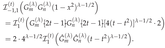 where is the Kronecker delta and is the normalization constant given by:
Proof.
The SG polynomials are defined in terms of standard Gegenbauer polynomials through the transformation:
Standard Gegenbauer polynomials are orthogonal on with respect to the weight function :
where
Substituting into the standard orthogonality relation:
Therefore:
where . This completes the proof of orthogonality. The completeness of the polynomial basis follows from standard results in approximation theory. □
Appendix A.2. Bijectivity of the RLFI Transformation
Theorem A9
(Bijectivity of the RLFI Transformation). For any fixed and , the mapping defined by is bijective. That is, it is both injective and surjective, establishing a perfect correspondence between the intervals and .
Proof.
A function is bijective if and only if it is both injective and surjective.
- 1.
-
Injectivity (One-to-One): Assume for . Then:Since , we can divide both sides by t:Thus, is injective.
- 2.
-
Surjectivity (Onto): , we need to find such that . Solving:Since , we have , so . Raising both sides to the power :Thus, . Therefore, is surjective.
- 3.
-
Explicit Inverse: The inverse function is explicitly given by:This confirms the bijection since a function is bijective if and only if it has an inverse.
- 4.
-
Boundary Behavior:
- By definition: As , ; as , .
- By injectivity and the inverse function: As , ; as , .
Thus, the mapping preserves the open intervals: .
□
Corollary A2
(Diffeomorphism Property). The transformation (2) constitutes a -diffeomorphism between and . Specifically, it has non-vanishing Jacobian
and both and its inverse
are on their respective domains.
Proof.
For fixed and , the map is well-defined and real-analytic on . Hence (2) is real-analytic, in particular . Differentiating (2) with respect to y gives (A46). Since , , and , we have , so
By Theorem A9, the mapping is bijective. Because is with non-vanishing derivative on , the inverse function theorem implies that the inverse map (A47) is also on . Thus is a -diffeomorphism between and . □
Appendix A.3. Smoothness Characterization of GBFA-Transformed Integrands and Its Implications for Convergence Rates
Theorem A10
(Exact Smoothness of the Transformed Integrand under the Classical GBFA Map). Let , , , and assume f is real-analytic on a neighborhood of . Define the transformed integrand
Set and . Then:
- (i)
- If (i.e., ), then and, generically, .
- (ii)
- If (i.e., ), then g is real-analytic on .
Proof.
Define . Since f is real-analytic on a neighborhood of and for all , the composition is real-analytic on by the chain rule.
To analyze regularity at , first note that for any and any ,
for some constant (and whenever or ). Thus
By Faà di Bruno’s formula [17],
where each monomial in is a product of powers of and scales as . The most singular contribution arises when , yielding asymptotically
Since as and generically, remains bounded near if and only if , i.e., .
We now distinguish two cases.
Case (i): . Then , so is continuous on , while for we have
which diverges as . Moreover,
so is Hölder-continuous of order at . Hence and, generically, .
Case (ii): . In this case is a polynomial, so is also a polynomial and therefore real-analytic on . Since f is real-analytic on a neighborhood of , the composition is real-analytic on . In particular, .
This completes the proof. □
The preceding analysis leads directly to the following corollary, formalizing the resulting regularity and quadrature behavior.
Corollary A3.
Let and define . Then the following hold:
- (i)
- If , then g is real-analytic on , and the -GBFA quadrature applied to the SG–transformed integrals in (6) converges super-exponentially in . If, in addition, f is a polynomial of degree d, then g is a polynomial of degree at most , and the quadrature is exact for all . Consequently, the total GBFA error reduces to the ITE, which vanishes for all , yielding exact evaluation of for every and .
- (ii)
- If , then with and , and generically ; cf. Theorem A10(i). In this case, the quadrature error decays algebraically as under Gauss-type rules.
Remark A9.
The algebraic rate in Corollary A3(ii) represents the worst-case convergence for arbitrary . However, if f is real-analytic on a neighborhood of , then the transformed integrand
admits a convergent fractional power series expansion near of the form
where with for some . Consequently, the coefficients satisfy for and , exhibiting exponential-type decay. This rapid decay implies that the tail of the series beyond indices is extremely small. As a result, Gauss-type quadrature rules–though asymptotically limited to an algebraic rate by the endpoint Hölder regularity–often exhibit dramatically faster pre-asymptotic convergence in practice. The observed convergence can thus appear nearly exponential or high-order algebraic over typical computational ranges (–), even though the strict asymptotic rate governs only the limit .
Appendix A.4. Diffeomorphism Property of the ϕ(α)-Mapping
We now formalize the smoothness and invertibility of the generalized RLFI transformation (35) introduced in Section 4. The result is the exact analogue of Corollary A2 for the mapping (2).
Theorem A11
(-diffeomorphism of the -mapping). Let , , and let be fixed. Consider the mapping
as defined in (35). Then τ is a -diffeomorphism between and ; that is,
- (i)
- τ is bijective,
- (ii)
- with
- (iii)
- its inverse ,belongs to .
Proof.
To prove the smoothness and non-vanishing Jacobian, notice that and , the map is real-analytic on ; thus the map (35) is real-analytic on , in particular . Differentiating (35) with respect to y yields
Since , , and , it follows that
The bijectivity proof argument parallels that of Theorem A9, but now for (35). In particular, to verify the map’s injectivity, assume for some . Then
Dividing by gives
since the map is strictly increasing on . Hence is injective. To prove surjectivity, let be arbitrary. We seek such that . Solving
for gives
Since , we have , hence
Thus, with , and is surjective. Combining injectivity and surjectivity, is bijective with inverse
The smoothness of the inverse follows by realizing that the map
is real-analytic on , and its image lies in . The map
with fixed, is real-analytic on . Therefore, their composition
is real-analytic on , in particular . In summary, we have shown that is bijective, with on , and its inverse y is on . Hence, by definition, is a -diffeomorphism between and . □
Appendix A.5. Smoothness of g via Faà di Bruno Exponent Analysis
Theorem A12
(Sufficient Smoothness Condition for ). Let , , and . Define
for . Then, for any , a sufficient condition for is
Proof.
Set and for brevity, and define . Then . Since and , g is smooth on . We analyze the behavior of as . By the Leibniz rule,
Step 1: The term. Repeated differentiation of shows that
for some finite constant (possibly zero only if and ). Since as and f is smooth on , we have
Thus, unless , the term behaves asymptotically as
for some constant . In particular, its exponent is . If , then this contribution either vanishes identically or is replaced by a term with a strictly larger exponent, which can only improve regularity at .
Step 2: The terms with . Each such term contains at least one derivative of the composition . By Faà di Bruno’s formula, we can write
where each monomial in the Bell polynomial is of the form
with nonnegative integers satisfying
Since as , the product scales as
Multiplying by gives a total factor of
Since and , we have
Thus every term with carries an exponent strictly larger than , and therefore decays faster as than the generic contribution.
Step 3: Boundedness of at . Combining the two steps, we see that, in the generic case where , the smallest exponent among all contributions to is . Hence the worst-case behaviour near is governed by
Appendix A.6. Gevrey Regularity of the Exact Solution (45)
We establish the precise smoothness class of the exact solution (45) of (44). Although u is real-analytic on , its derivatives grow factorially. We prove that u belongs to the Gevrey-1 class, which is equivalent to the class of real-analytic functions, but does not satisfy the derivative bound (9) required by Theorem 1.
Theorem A13
Proof.
The function is the restriction to of the complex function , which is analytic on . Since the singularity at is at a distance of 1 from , u is real-analytic on .
We now compute the kth derivative. For , the kth derivative of is
Using and , we obtain
Applying the property of the Gamma function [22, Eq. (6.1.12)],
and the bound for the double factorial , we can use Stirling’s approximation to find that there exist constants such that
Thus, for and , the bound (A49) holds. Consequently, u fails to meet the hypothesis of Theorem 1. □
References
- Podlubny, I. Fractional Differential Equations. In Academic Press.; 1999. [Google Scholar]
- Mainardi, F. Fractional Calculus and Waves in Linear Viscoelasticity. In World Scientific; 2022. [Google Scholar]
- Metzler, R.; Klafter, J. The random walk’s guide to anomalous diffusion: A fractional dynamics approach. Physics Reports 2000, 339(1), 1–77. [Google Scholar]
- Elgindy, K. T. Super-exponential approximation of the Riemann–Liouville fractional integral via Gegenbauer-based fractional approximation methods. Algorithms 2025, 18, 395. [Google Scholar]
- Diethelm, K.; Ford, N. J.; Freed, A. D.; Luchko, Y. Algorithms for the fractional calculus: A selection of numerical methods. Computer Methods in Applied Mechanics and Engineering 2005, 194(6-8), 743–773. [Google Scholar] [CrossRef]
- Avcı, İ.; Mahmudov, N. I. Numerical solutions for multi-term fractional order differential equations with fractional Taylor operational matrix of fractional integration. Mathematics 2020, 8(1), 96. [Google Scholar] [CrossRef]
- Krishnasamy, V. S.; Mashayekhi, S.; Razzaghi, M. Numerical solutions of fractional differential equations by using fractional Taylor basis. IEEE/CAA Journal of Automatica Sinica 2017, 4(1), 98–106. [Google Scholar] [CrossRef]
- Zhang, J.; Zhou, F.; Mao, N. Numerical optimization algorithm for solving time-fractional telegraph equations. Physica Scripta 2025, 100(4), 045237. [Google Scholar] [CrossRef]
- Ghasempour, A.; Ordokhani, Y.; Sabermahani, S. Mittag-Leffler wavelets and their applications for solving fractional optimal control problems. Journal of Vibration and Control 2025, 31(5-6), 753–767. [Google Scholar]
- Shen, J.; Tang, T.; Wang, L.-L. Spectral Methods: Algorithms, Analysis and Applications. In Springer; 2011. [Google Scholar]
- Canuto, C.; Hussaini, M. Y.; Quarteroni, A.; Zang, T. A. Spectral Methods: Fundamentals in Single Domains. In Springer Science & Business Media; 2012. [Google Scholar]
- Elgindy, K. T. Gegenbauer Collocation Integration Methods: Advances in Computational Optimal Control Theory. PhD thesis, Monash University., 2013. [Google Scholar]
- Zhang, T.-F.; Yin, Z. Gevrey regularity for solutions of the non-cutoff Boltzmann equation: The spatially inhomogeneous case. Nonlinear Analysis: Real World Applications 2014, 15, 246–261. [Google Scholar] [CrossRef]
- Jackson, D. The Theory of Approximation; American Mathematical Society Colloquium Publications, 1930; Volume 11. [Google Scholar]
- Xiang, S. On interpolation approximation: Convergence rates for polynomial interpolation for functions of limited regularity. SIAM Journal on Numerical Analysis 2016, 54(4), 2081–2113. [Google Scholar] [CrossRef]
- Elgindy, K. T. High-order, stable, and efficient pseudospectral method using barycentric Gegenbauer quadratures. Applied Numerical Mathematics 2017, 113, 1–25. [Google Scholar] [CrossRef]
- Johnson, W. P. The curious history of Faá di Bruno’s formula. The American Mathematical Monthly 2002, 109(3), 217–234. [Google Scholar]
- Ghorbani, K.; Semperlotti, F. On the one-dimensional SPH approximation of fractional-order operators. arXiv 2025, arXiv:2505.04350. [Google Scholar]
- Damarla, S. K.; Kundu, M. Novel hybrid function operational matrices of fractional integration: An application for solving multi-order fractional differential equations. AppliedMath 2025, 5(2), 55. [Google Scholar] [CrossRef]
- Usta, F. Numerical analysis of fractional Volterra integral equations via Bernstein approximation method. Journal of Computational and Applied Mathematics 2021, 384, 113198. [Google Scholar] [CrossRef]
- Micula, S. An iterative numerical method for fractional integral equations of the second kind. Journal of Computational and Applied Mathematics 2018, 339, 124–133. [Google Scholar] [CrossRef]
- Abramowitz, M.; Stegun, I. A. Handbook of Mathematical Functions with Formulas, Graphs, and Mathematical Tables. In US Government Printing Office; 1948; Vol. 55. [Google Scholar]
- Kumar, K.; Pandey, R. K.; Sharma, S. Approximations of fractional integrals and Caputo derivatives with application in solving Abel’s integral equations. Journal of King Saud University-Science 2019, 31(4), 692–700. [Google Scholar] [CrossRef]
- Rao, N.; Farid, M.; Jha, N. K. Approximation properties of a fractional integral-type Szász–Kantorovich–Stancu–Schurer operator via Charlier polynomials. Mathematics 2025, 13(18), 3039. [Google Scholar] [CrossRef]
- Ciesielski, M.; Grodzki, G. Numerical approximations of the Riemann–Liouville and Riesz fractional integrals. Informatica 2024, 35(1), 21–46. [Google Scholar] [CrossRef]
- Ciesielski, M. Numerical algorithms for approximation of fractional integrals and derivatives based on quintic spline interpolation. Symmetry 2024, 16(2), 252. [Google Scholar] [CrossRef]
- Batiha, I. M.; Saadeh, R.; Jebril, I. H.; Qazza, A.; Al-Nana, A. A.; Momani, S. Composite fractional trapezoidal rule with Romberg integration. Computer Modeling in Engineering & Sciences 2024, 140(3), 2729–2745. [Google Scholar] [CrossRef]
- Batiha, I. M.; Alshorm, S.; Al-Husban, A.; Saadeh, R.; Gharib, G.; Momani, S. The n-point composite fractional formula for approximating Riemann–Liouville integrator. Symmetry 2023, 15(4), 938. [Google Scholar] [CrossRef]
- Butt, S. I.; Khan, D.; Tipurić-Spužević, S.; Mohsin, B. B. Fractional perspective of HH f-divergence, midpoint and trapezoidal type estimates for superquadratic function. Kuwait Journal of Science 2025, 100452. [Google Scholar] [CrossRef]
- Bouafoura, M. K.; Braiek, N. B. Block pulse-based techniques for modelling and synthesis of non-integer systems. International Journal of Systems Science 2010, 41(5), 487–499. [Google Scholar] [CrossRef]
- Postavaru, O.; Toma, A. A numerical approach based on fractional-order hybrid functions of block-pulse and Bernoulli polynomials for numerical solutions of fractional optimal control problems. Mathematics and Computers in Simulation 2022, 194, 269–284. [Google Scholar] [CrossRef]
- Barary, Z.; Yazdani Cherati, A.; Nemati, S. Solving fractional optimal control-affine problems via fractional-order hybrid Jacobi functions. Control and Optimization in Applied Mathematics 2024, 9(1), 149–168. [Google Scholar]
- Sadek, L.; Ounamane, S.; Abouzaid, B.; Sadek, E. M. The Galerkin Bell method to solve the fractional optimal control problems with inequality constraints. Journal of Computational Science 2024, 77, 102244. [Google Scholar] [CrossRef]
- Mohammadi, H.; Saeedi, H.; Izadi, M. A spectral collocation method via Krawtchouk polynomials for two-dimensional Liouville–Caputo fractional optimal control problems. Results in Control and Optimization 2025, 100639. [Google Scholar] [CrossRef]
- Shadimetov, K.; Nuraliev, F.; Toshboev, O. Optimal methods for approximate calculation of the fractional Riemann-Liouville integral in Sobolev space. AIP Conference Proceedings 2024, 3147(1). [Google Scholar] [CrossRef]
- Zhou, Z.; Zhang, H.; Yang, X. The compact difference scheme for the fourth-order nonlocal evolution equation with a weakly singular kernel. Mathematical Methods in the Applied Sciences 2023, 46(5), 5422–5447. [Google Scholar] [CrossRef]
- Okayama, T.; Matsuo, T.; Sugihara, M. Sinc-collocation methods for weakly singular Fredholm integral equations of the second kind. Journal of Computational and Applied Mathematics 2010, 234(4), 1211–1227. [Google Scholar] [CrossRef]
- Galperin, E. A.; Kansa, E. J.; Makroglou, A.; Nelson, S. A. Variable transformations in the numerical solution of second kind Volterra integral equations with continuous and weakly singular kernels; extensions to Fredholm integral equations. Journal of Computational and Applied Mathematics 2000, 115(1-2), 193–211. [Google Scholar] [CrossRef]
- Baumann, G.; Stenger, F. Fractional calculus and Sinc methods. Fractional Calculus and Applied Analysis 2011, 14(4), 568–622. [Google Scholar] [CrossRef]
- Hussien, H. S.; Abdalla, M. Spectral optimal control solution for nonlinear weakly singular system of fractional integro-differential equations. Fractals 2025, 33(08), 1–11. [Google Scholar] [CrossRef]
- Taleshian, A. H.; Nemati, S.; Lima, P. M. Application of fractional-order hybrid Chelyshkov functions for solving a general class of fractional integro-differential equations with weakly singular kernels. Journal of Computational and Applied Mathematics 2025, 117110. [Google Scholar] [CrossRef]
- Al Jarbouh, A. Rheological behaviour modelling of viscoelastic materials by using fractional model. Energy Procedia 2012, 19, 143–157. [Google Scholar] [CrossRef]
- Anwar, M. S.; Alam, M. M.; Khan, M. A.; Abouzied, Amr S.; Hussain, Z.; Puneeth, V. Generalized viscoelastic flow with thermal radiations and chemical reactions. Geoenergy Science and Engineering 2024, 232, 212442. [Google Scholar] [CrossRef]
- Geetanjali, G.; Sharma, P. K. Fractional order strain and viscosity in the Moore Gibson Thompson thermoelastic diffusion model: A study of transient responses in one-dimensional half-space. Mechanics of Materials 2025, 105542. [Google Scholar] [CrossRef]
- Mescia, L.; Bia, P.; Caratelli, D. Fractional-calculus-based electromagnetic tool to study pulse propagation in arbitrary dispersive dielectrics. Physica Status Solidi (a) 2019, 216(3), 1800557. [Google Scholar] [CrossRef]
- Xu, K.; Chen, L.; Wang, M.; Lopes, A. M.; Tenreiro Machado, J. A.; Zhai, H. Improved decentralized fractional PD control of structure vibrations. Mathematics 2020, 8(3), 326. [Google Scholar] [CrossRef]
- Jiang, Y.; Zhang, B.; Shu, X.; Wei, Z. Fractional-order autonomous circuits with order larger than one. Journal of Advanced Research 2020, 25, 217–225. [Google Scholar] [CrossRef]
- Krejcar, O.; Namazi, H. Review of the applications of different fractional models in engineering. Applied Mathematical Modelling 2025, 116623. [Google Scholar] [CrossRef]
- Nemati, S.; Sedaghat, S.; Arefi, S. A new numerical approach for solving space–time fractional Schrödinger differential equations via fractional-order Chelyshkov functions. Results in Applied Mathematics 2025, 26, 100584. [Google Scholar] [CrossRef]
- Talib, I.; Özger, F. Orthogonal polynomials based operational matrices with applications to Bagley-Torvik fractional derivative differential equations. In Recent Research in Polynomials (Chap. 3); Özger, F., Ed.; IntechOpen., 2023. [Google Scholar]
- Mohammadi, F. A discrete orthogonal polynomials approach for fractional optimal control problems with time delay. Iranian Journal of Numerical Analysis and Optimization 2019, 9(2), 49–75. [Google Scholar]
- Wang, M. L.; Chang, R. Y.; Yang, S. Y. Generalization of generalized orthogonal polynomial operational matrices for fractional and operational calculus. International Journal of Systems Science 1987, 18(5), 931–943. [Google Scholar] [CrossRef]
- Grodzki, G. Numerical approximation of the Riemann-Liouville fractional integrals using the Akima spline interpolation. Journal of Applied Mathematics and Computational Mechanics 2023, 22(4), 30–43. [Google Scholar] [CrossRef]
- Bhrawy, A. H.; Alofi, A. S. The operational matrix of fractional integration for shifted Chebyshev polynomials. Applied Mathematics Letters 2013, 26(1), 25–31. [Google Scholar] [CrossRef]
- Ghasempour, A.; Ordokhani, Y.; Sabermahani, S. Mittag-Leffler wavelets and their applications for solving fractional optimal control problems. Journal of Vibration and Control 2025, 31(5-6), 753–767. [Google Scholar] [CrossRef]
- Sidi, A. A new variable transformation for numerical integration. In Numerical Integration IV: Proceedings of the Conference at the Mathematical Research Institute, Oberwolfach, November 8–14, 1992; Springer., 1993; pp. 359–373. [Google Scholar]
- Laurie, D. P. Periodizing transformations for numerical integration. Journal of Computational and Applied Mathematics 1996, 66(1-2), 337–344. [Google Scholar] [CrossRef]
- Elgindy, K. T. High-order numerical solution of second-order one-dimensional hyperbolic telegraph equation using a shifted Gegenbauer pseudospectral method. Numerical Methods for Partial Differential Equations 2016, 32(1), 307–349. [Google Scholar] [CrossRef]
Figure 1.
Behavior of the bounding constant as varies from to 5, shown for six representative values of (, 0, , 1, 2, and 3). Each curve corresponds to a distinct value: red (), dark green (), blue (), purple (), orange (), and black ().
Figure 1.
Behavior of the bounding constant as varies from to 5, shown for six representative values of (, 0, , 1, 2, and 3). Each curve corresponds to a distinct value: red (), dark green (), blue (), purple (), orange (), and black ().
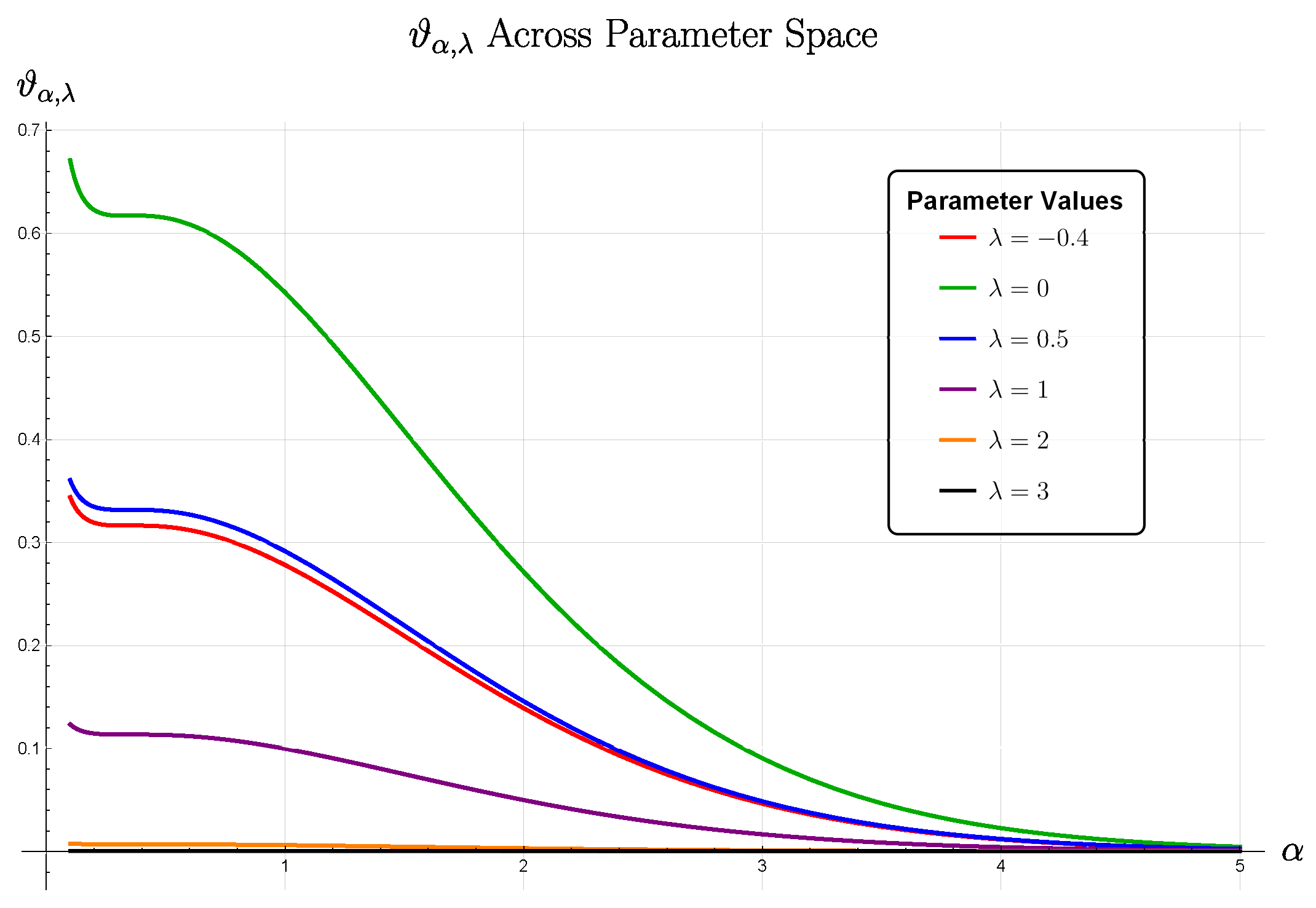
Figure 2.
Effect of the smoothness parameter r on the transformed integrand for and two representative values of (left: , right: ). Top row: ; bottom row: . For both values, increasing r improves the smoothness of g at but simultaneously concentrates the integrand increasingly near , as visible from the steeper decay toward and the sharper peaks near .
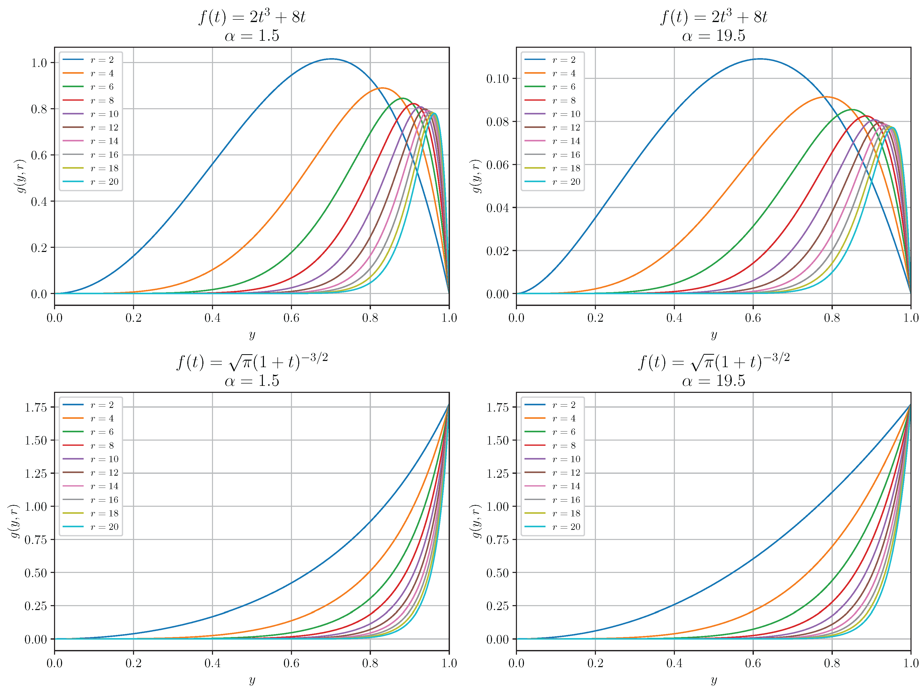
Figure 3.
Comprehensive RLFI analysis for at : (a) GBFA approximation versus exact RLFI values across ; (b) LARE versus ; (c) LARE versus interpolation degree n for multiple values; (d) LARE versus SG parameter for multiple values; (e) LARE versus quadrature parameter for multiple values; (f) LARE versus quadrature points for multiple values. In all panels, markers show computed data points, and lines connect points for visual clarity. Each color represents a different value as indicated in the legends.
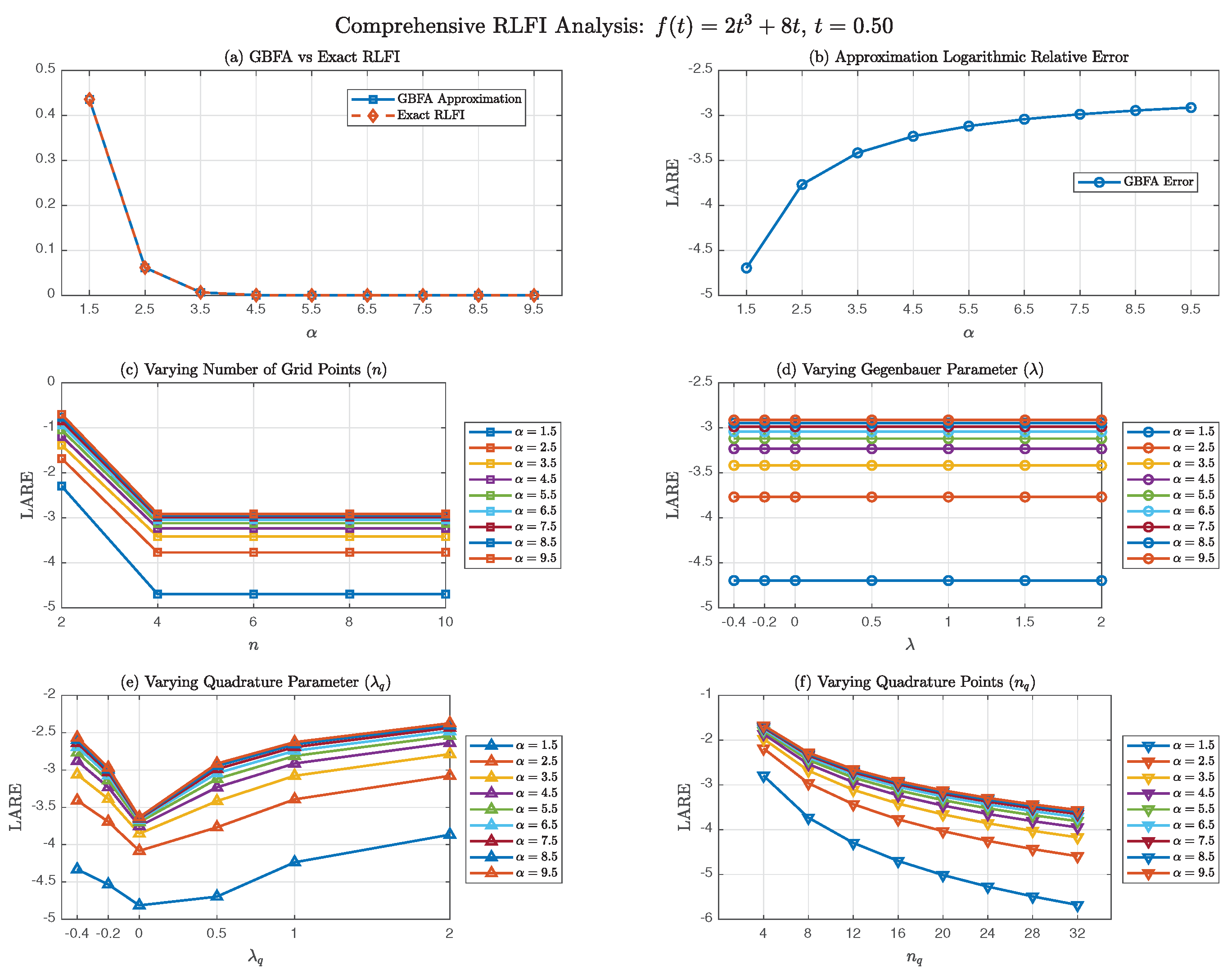
Figure 4.
Comprehensive RLFI analysis for at with extended quadrature resolution: (a) LARE versus interpolation degree n for multiple values using ; (b) LARE versus SG parameter for multiple values using ; (c) LARE versus quadrature parameter for multiple values using ; (d) LARE versus quadrature points on a logarithmic scale for multiple values, with ranging from 4 to . In all panels, markers show computed data points, and lines connect points for visual clarity. Each color represents a different value as indicated in the legends.
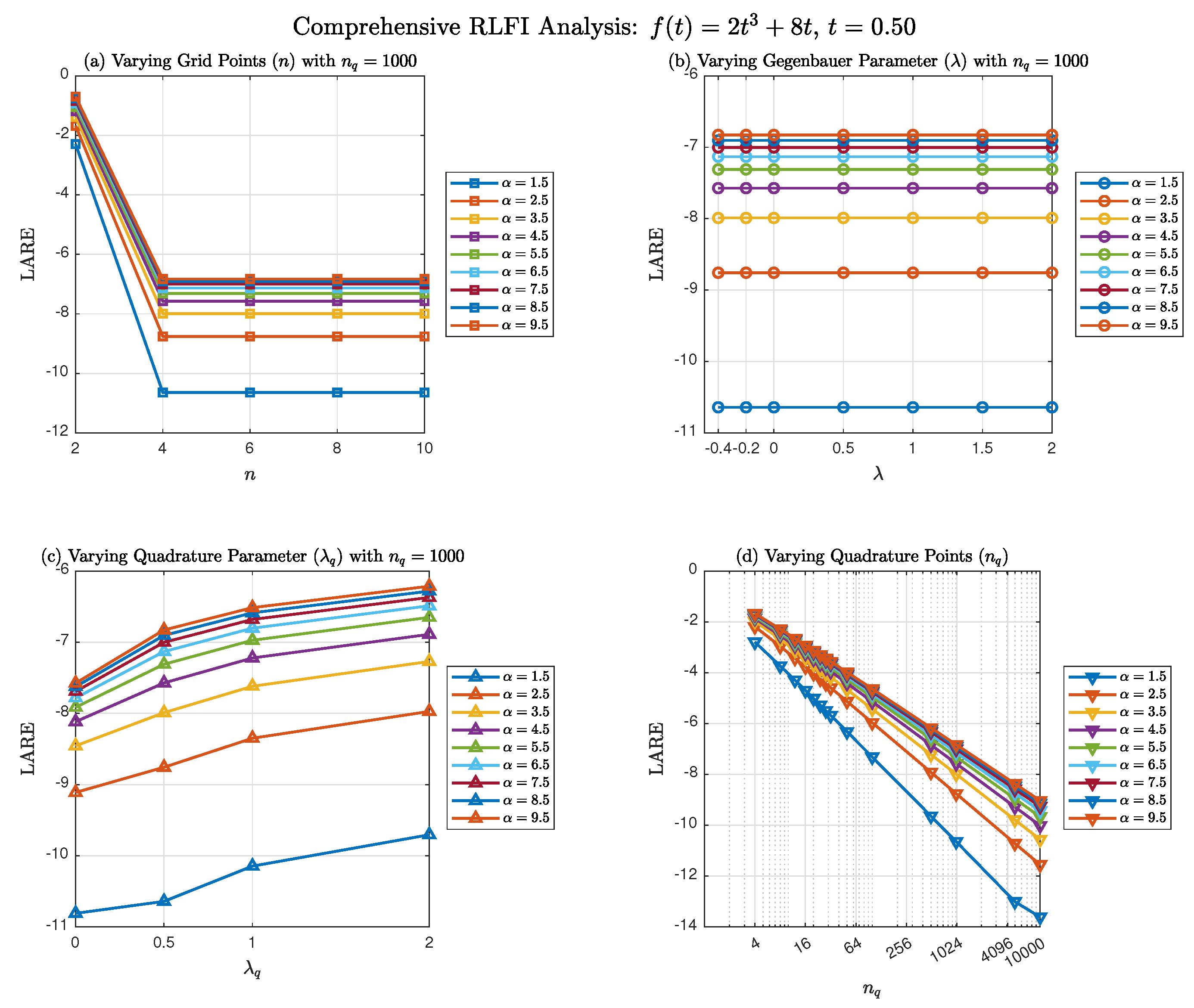
Figure 5.
Comprehensive RLFI analysis for at using the -generalized transformation with : (a) GBFA approximation versus exact RLFI values across ; (b) LARE versus ; (c) LARE versus interpolation degree n for multiple values; (d) LARE versus SG parameter for multiple values; (e) LARE versus quadrature parameter for multiple values; (f) LARE versus quadrature points for multiple values. In all panels, markers show computed data points, and lines connect points for visual clarity. Each color represents a different value as indicated in the legends.
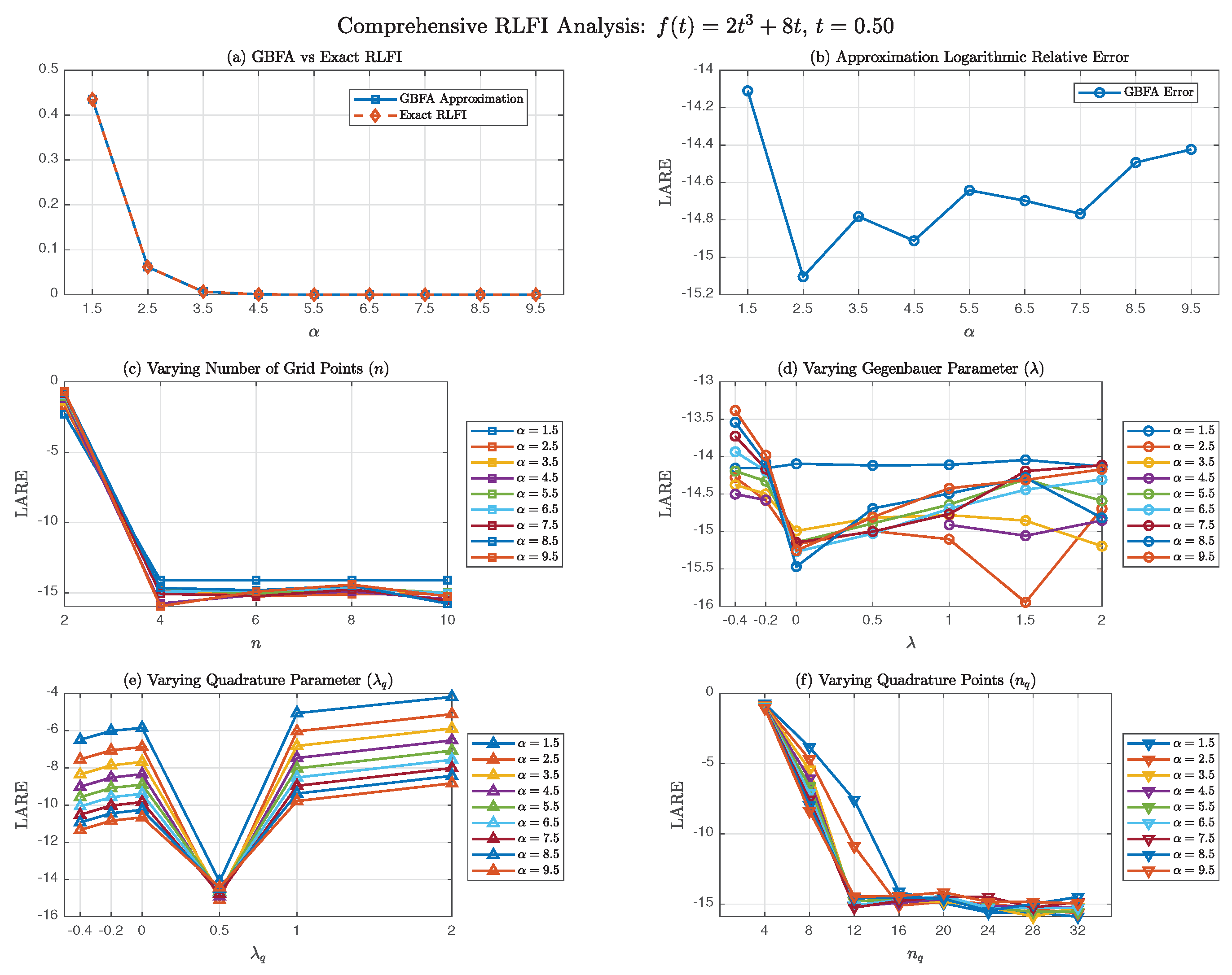
Figure 6.
Three-dimensional sensitivity analysis of the -generalized transformation with respect to smoothness parameter r: (a) LARE vs. r vs. for fixed ; (b) LARE vs. r vs. for fixed ; (c) LARE vs. r vs. for fixed .
Figure 6.
Three-dimensional sensitivity analysis of the -generalized transformation with respect to smoothness parameter r: (a) LARE vs. r vs. for fixed ; (b) LARE vs. r vs. for fixed ; (c) LARE vs. r vs. for fixed .
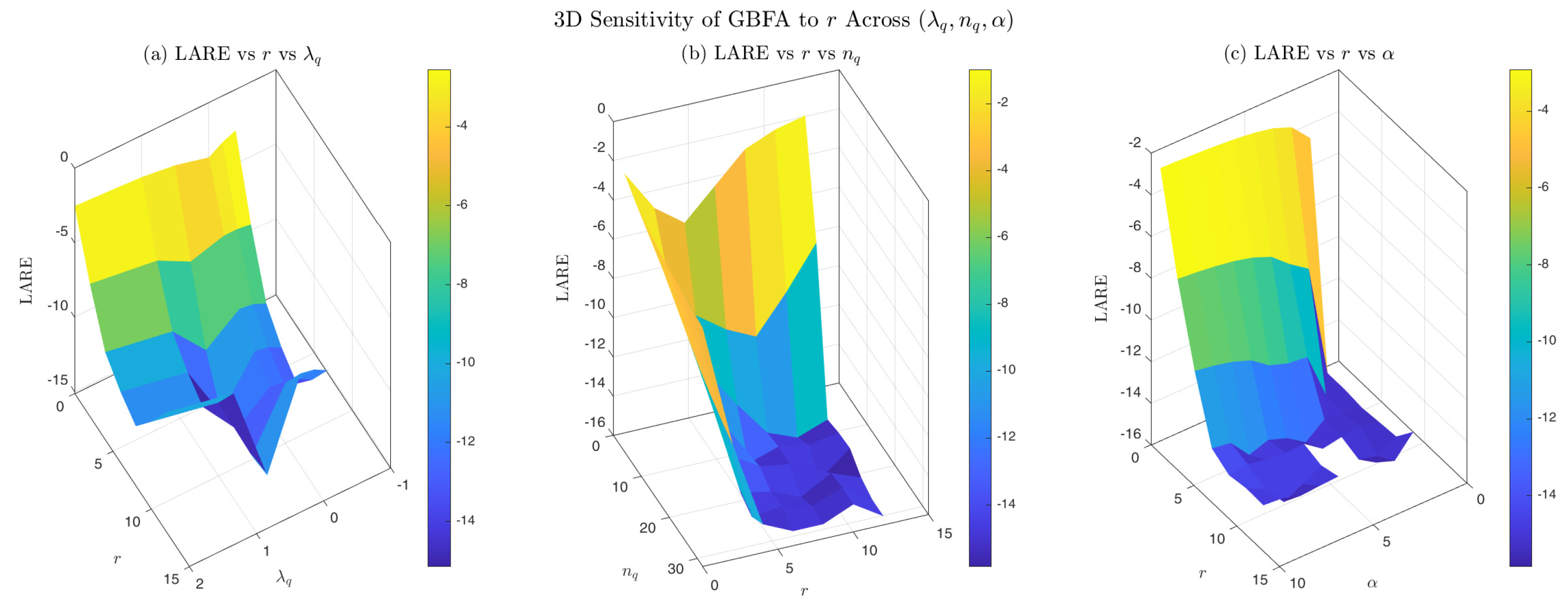
Figure 7.
Accuracy comparison between GBFA (-generalized, ) and MATLAB integral for , : (a) RLFI values versus ; (b) LARE versus . The GBFA method uses , , , ; MATLAB uses relative tolerance . Both methods achieve near machine-precision accuracy over .
Figure 7.
Accuracy comparison between GBFA (-generalized, ) and MATLAB integral for , : (a) RLFI values versus ; (b) LARE versus . The GBFA method uses , , , ; MATLAB uses relative tolerance . Both methods achieve near machine-precision accuracy over .
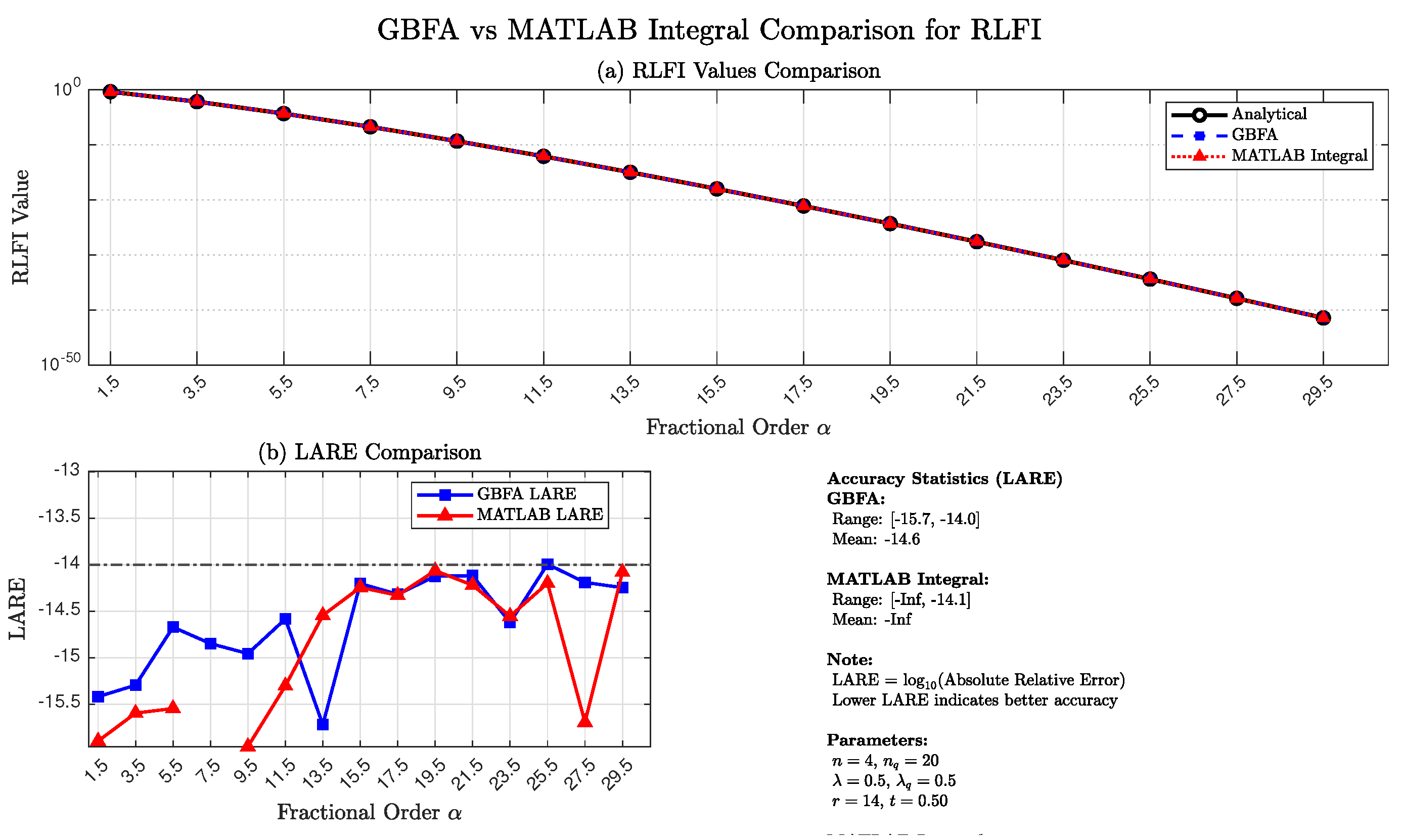
Figure 8.
Computational efficiency comparison between GBFA (-generalized, ) and MATLAB integral: (a) Computation time in microseconds versus ; (b) Speedup factor (MATLAB time / GBFA time) versus . The GBFA method exhibits evaluation times under after FSGIM precomputation, while MATLAB requires 193–. Speedup factors range from to over .
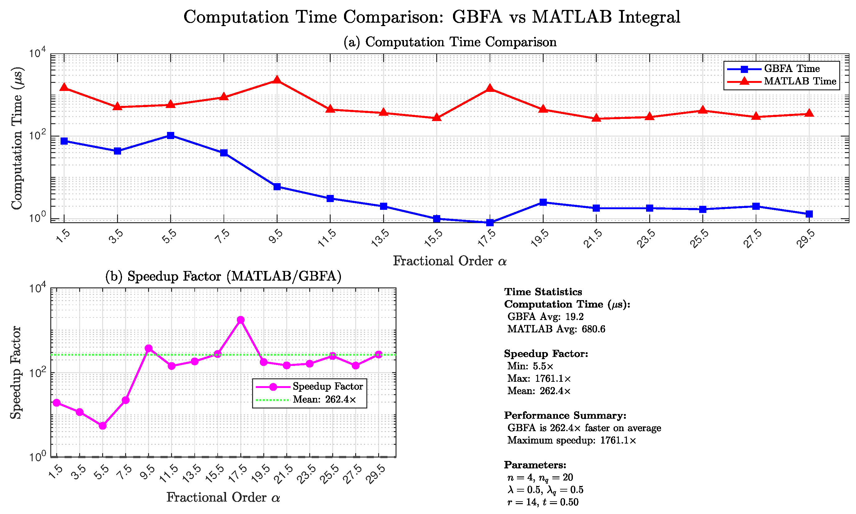
Figure 9.
GBFA approximation of for (a1) , (a2) , (a3) , and (a4) on , with corresponding error distributions in (b1)–(b4). The left panels show GBFA and exact RLFI values; the right panels show pointwise absolute error (blue), mean error (red dashed), and median error (magenta dash-dotted).
Figure 9.
GBFA approximation of for (a1) , (a2) , (a3) , and (a4) on , with corresponding error distributions in (b1)–(b4). The left panels show GBFA and exact RLFI values; the right panels show pointwise absolute error (blue), mean error (red dashed), and median error (magenta dash-dotted).
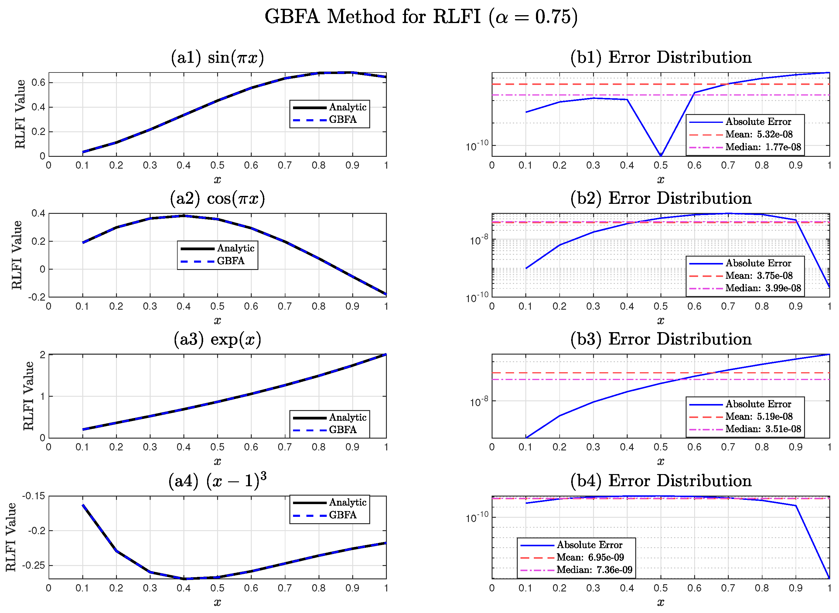
Figure 10.
Error metrics for the GBFA approximation of on : (a) error; (b) score; (c) maximum vs. mean absolute error; (d) comparison of MAE, mean, median, and . All errors are below , and scores exceed .
Figure 10.
Error metrics for the GBFA approximation of on : (a) error; (b) score; (c) maximum vs. mean absolute error; (d) comparison of MAE, mean, median, and . All errors are below , and scores exceed .
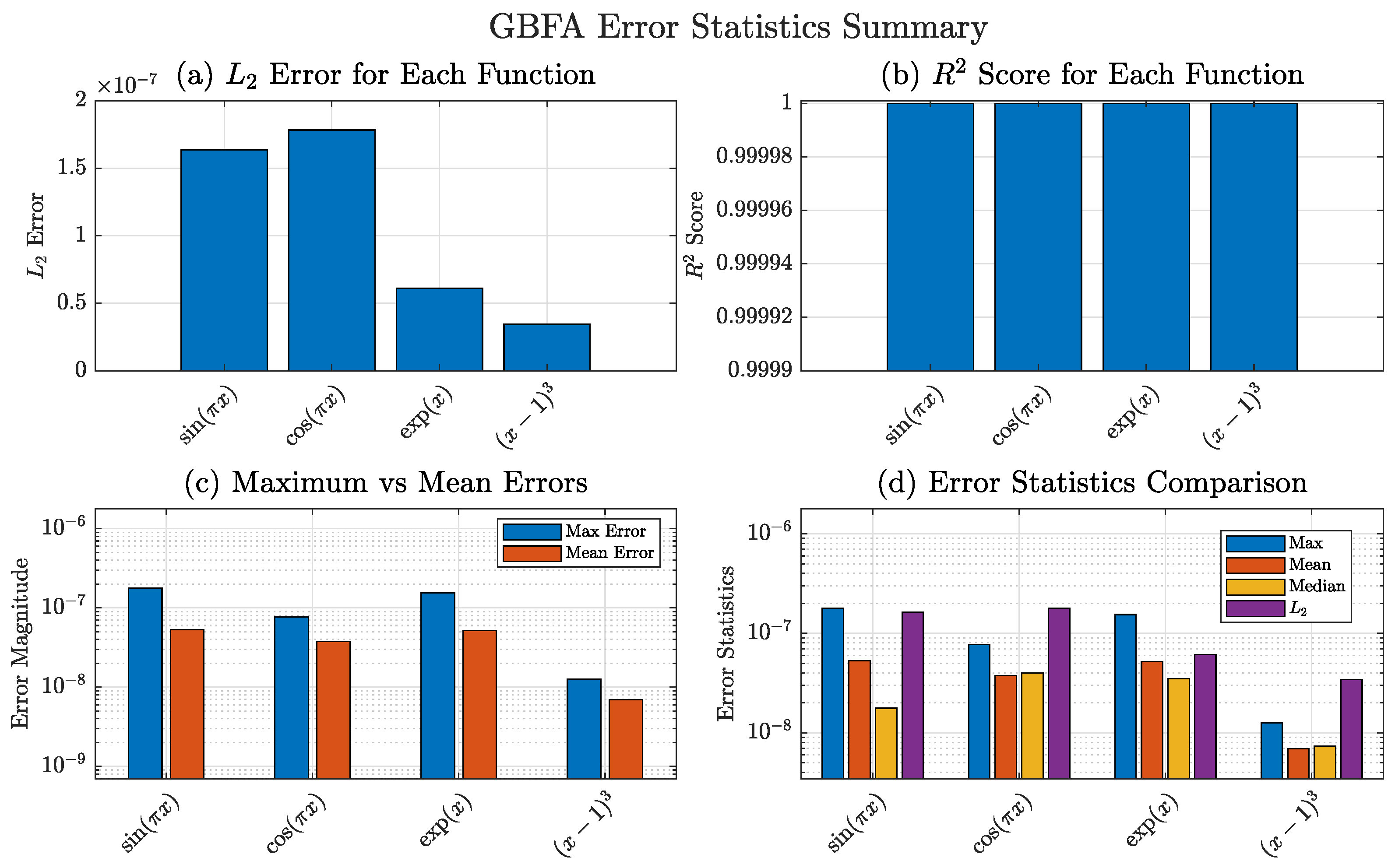
Figure 11.
Convergence of the GBFA method for at using the classical transformation . Absolute error versus quadrature order (blue circles), best-fit algebraic rate (red dashed), and theoretical asymptotic rate (black dotted). The rapid pre-asymptotic decay reflects the exponential coefficient decay in the fractional power series of the transformed integrand, despite the endpoint Hölder regularity .
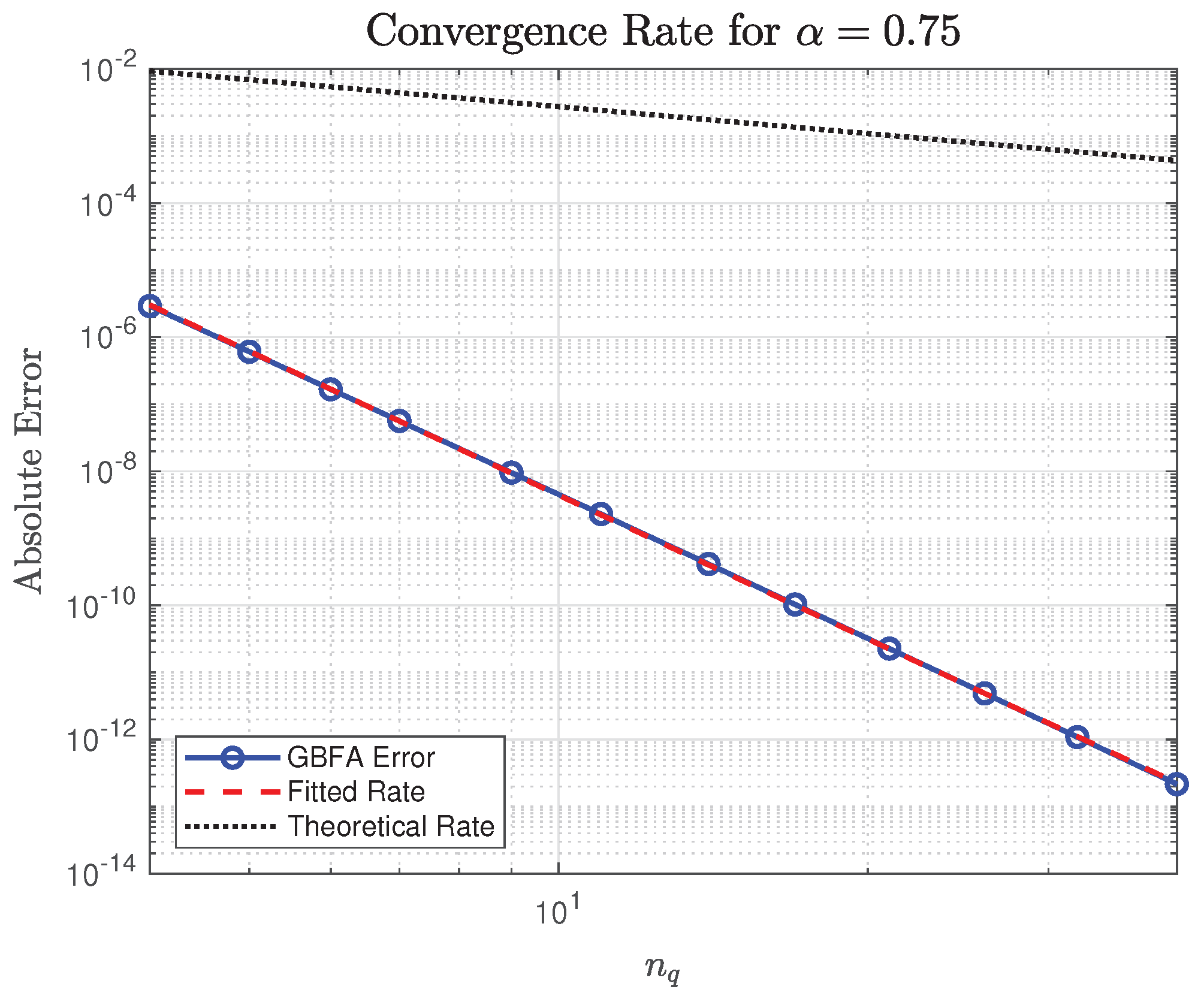
Figure 12.
Convergence of the GBFA method for at using the -generalized transformation with . Absolute error versus quadrature order (blue circles), best-fit algebraic rate (red dashed), and theoretical rate (black dotted). The asymptotic regime is attained only for , beyond which the generalized map overtakes the classical one in convergence speed–but at the cost of degraded pre-asymptotic accuracy and increased sensitivity to .
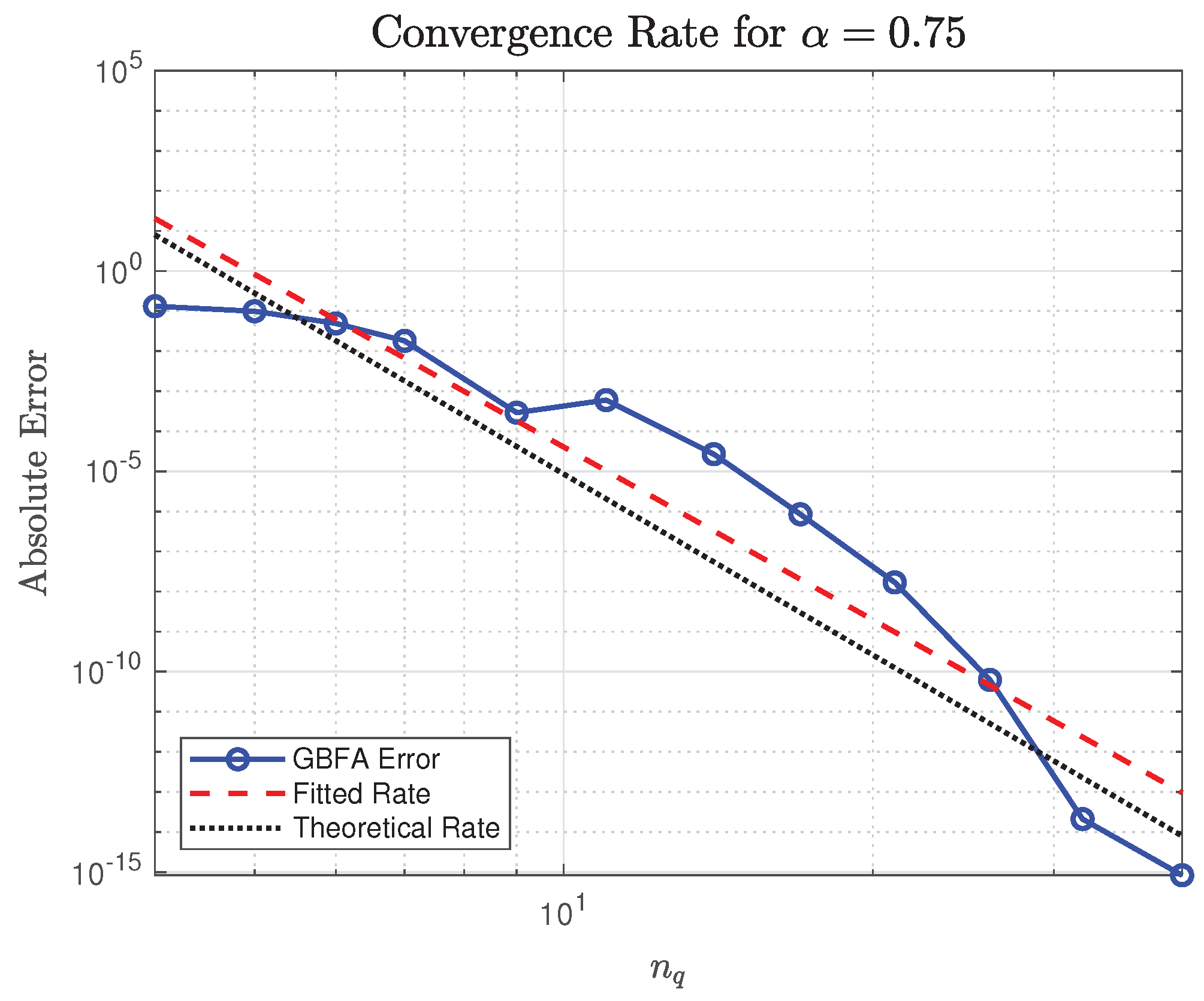
Figure 13.
GBFA solution of the 2nd FVIE (44) vs. exact solution. Markers: SGG nodes ().
Figure 13.
GBFA solution of the 2nd FVIE (44) vs. exact solution. Markers: SGG nodes ().
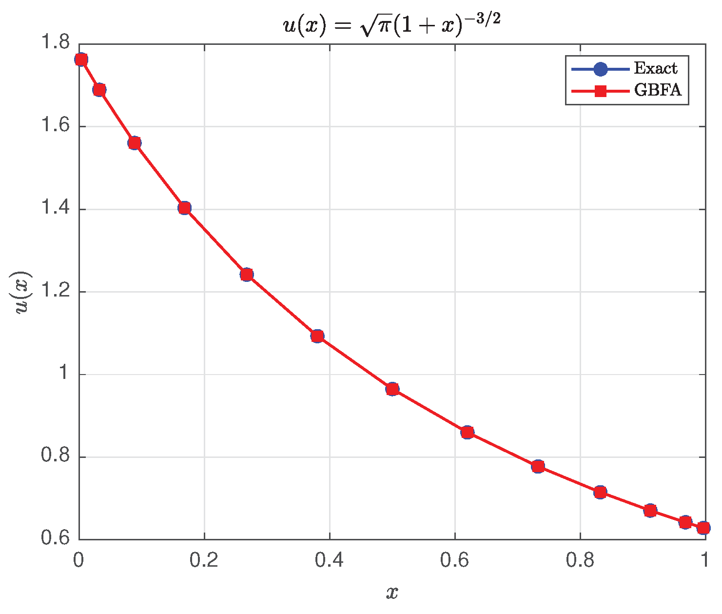
Figure 14.
Convergence rate of GBFA for solving Eq. (44): MAE vs. polynomial degree n.
Figure 14.
Convergence rate of GBFA for solving Eq. (44): MAE vs. polynomial degree n.
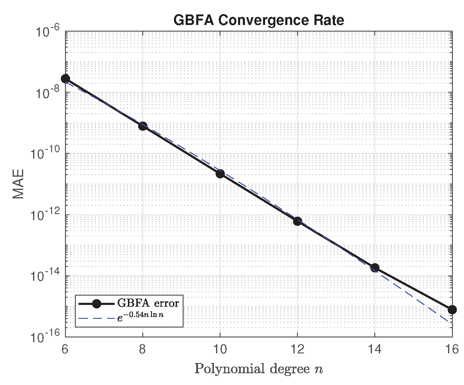
Table 1.
Estimated MAE of SPH [18] and GBFA for on . The SPH values are inferred from [18, Fig. 5]; GBFA uses , .
| Function | SPH MAE (estimated) | GBFA MAE | GBFA Error |
Table 2.
Comparison of GBFA and HF [19] for with on the HF grid . The GBFA parameters are , , , .
Table 2.
Comparison of GBFA and HF [19] for with on the HF grid . The GBFA parameters are , , , .
| GBFA | HF [19] | GBFA CPU (s) | HF CPU (s) [19] | Speedup | |
| 0.5 | |||||
| 1.0 | 0 | ||||
| 1.5 | |||||
| 2.0 | |||||
| 2.5 | |||||
| 3.0 | |||||
| 3.5 | |||||
| 4.0 | 0 | ||||
| 4.5 | |||||
| 5.0 |
| Method | n | MAE | RmsE | Time (s) |
| GBFA | 12 | |||
| Bernstein [20] | 12 |
Table 4.
Convergence data for GBFA applied to solve Eq. (44).
Table 4.
Convergence data for GBFA applied to solve Eq. (44).
| n | MAE | ln(MAE) |
| 6 | ||
| 8 | ||
| 10 | ||
| 12 | ||
| 14 | ||
| 16 |
Disclaimer/Publisher’s Note: The statements, opinions and data contained in all publications are solely those of the individual author(s) and contributor(s) and not of MDPI and/or the editor(s). MDPI and/or the editor(s) disclaim responsibility for any injury to people or property resulting from any ideas, methods, instructions or products referred to in the content. |
© 2026 by the authors. Licensee MDPI, Basel, Switzerland. This article is an open access article distributed under the terms and conditions of the Creative Commons Attribution (CC BY) license (http://creativecommons.org/licenses/by/4.0/).
Copyright: This open access article is published under a Creative Commons CC BY 4.0 license, which permit the free download, distribution, and reuse, provided that the author and preprint are cited in any reuse.


