
Submitted:
20 October 2025
Posted:
21 October 2025
You are already at the latest version
Abstract
Difference schemes for the numerical solution of fractional differential equations rely on discretizations of the fractional derivative. In earlier work \cite{d24}, we constructed approximations of the first derivative and applied them to fractional derivatives. In this paper, we extend the method from \cite{d24} to develop parameter-dependent approximations of the second derivative and second-order approximations of the fractional derivative based on the weights of the L1 scheme. We derive the second-order expansion formula of the L1 approximation and show that the coefficient of the second derivative is asymptotically equal to a value of the zeta function, as suggested by the generating function. Using this expansion, we construct a second-order approximation of the fractional derivative and the corresponding asymptotic approximation by a suitable choice of parameter. Examples illustrating the application of these approximations to the numerical solution of ordinary differential equations and fractional differential equations are presented. Both approximations of the fractional derivative are shown to yield second-order numerical methods. Numerical experiments are also provided, confirming the theoretical predictions for the accuracy order of the methods.
Keywords:
fractional derivative
; approximation
; numerical solution
; convergence
1. Introduction
Fractional differentiation extends integer-order differentiation and integration to arbitrary orders. There is a growing interest in developing numerical methods for fractional differential equations due to their wide applicability in various branches of science [2,3,4]. Finite difference schemes provide a powerful approach for the numerical solution of fractional differential equations and the study of their properties. The Caputo fractional derivative of order , where , is defined as
The power function and the functions , , and have fractional derivatives.
where and is the Mittag-Leffler function
The lower limit of fractional differentiation may be an arbitrary number. The kernel of the fractional derivative has a singularity of order . A direct application of numerical integration methods for discretizations of the fractional derivative leads to reduced accuracy and a lower order of approximation. Therefore, the construction of high-order approximations of fractional derivatives requires additional considerations.
Fractional calculus is a rapidly developing scientific field that extends and generalizes differential calculus. Other definitions of fractional derivatives and integrals include the Riemann–Liouville and Grünwald–Letnikov derivatives, introduced in the 19th century. The Riemann–Liouville derivative is the first known generalization of integer-order derivatives and is a widely used definition in fractional calculus. The three definitions of the fractional derivative are directly related and share similar properties. The main difference between fractional and integer-order derivatives lies in their nonlocal properties. Fractional derivatives have a strong dependence on the previous values of the function according to the power law, or exhibit memory-influenced dynamics. The definition of integer-order derivatives depends only on the local behavior of the function in a small neighborhood around the point of differentiation. The definitions of integer-order derivatives imply an exponential dependence on previous values, and this effect may be negligible or minimal. The choice of a particular definition of the fractional derivative and its advantages depend on the problem under consideration. The Caputo fractional derivative, defined in 1967, has the advantage that when solving differential equations, it allows the use of initial conditions expressed in terms of integer-order derivatives, which often have direct physical meaning. In addition to the most commonly used definitions of the fractional derivative, such as those of Riemann–Liouville and Caputo, there exist other important and widely applicable definitions in the theory of fractional calculus. Among them are the fractional derivatives of Weyl, Hadamard, Marchaud, and Riesz. The recently introduced fractional derivatives, the Caputo–Fabrizio derivative (2015), the Atangana–Baleanu–Caputo (ABC) fractional derivative (2016), have also proven their significance in modeling various time-dependent complex processes. These derivatives, provide improved accuracy in describing memory effects in physical, biological, and engineering phenomena [5,6,7].
Fractional Differential Equations (FDEs) are a generalization of ordinary and partial differential equations and provide powerful tools for modeling complex systems with memory, hereditary properties, or anomalous diffusion. Due to the complexity of fractional differential equations and their corresponding models, numerical methods are the main and, in many cases, the only approach for solving them. Numerical methods could be applied to a much wider class of fractional differential equations compared to analytical methods. Many of the properties and approaches used for solving ordinary and partial differential equations are also applicable to the corresponding fractional differential equations. The development of numerical methods is based on the growing number and diversity of the considered models, as well as on the improvement of the technical means for their solution. The main types of approaches for solving differential and fractional differential equations include the Finite Difference Methods [8,9,10,11], Spectral Methods [12,13,14,15], Finite Element Methods [16,17], and Predictor–Corrector Methods [18,19].
Finite difference schemes for the numerical solution of fractional differential equations are widely used because of their simplicity, flexibility, and consistency of the numerical results. The difference schemes for fractional differential equations use discretizations of the fractional derivative on uniform or nonuniform grids over the interval of fractional differentiation. These approximations involve the previous values of the function, which leads to a more complex analysis of the difference schemes and increases the computational time required for their solution. Constructions of fast difference schemes for fractional differential equations that achieve optimal computational complexity using sum of exponentials approximation of the kernel function are presented in [20,21,22,23]. To improve the efficiency of difference schemes and achieve high computational accuracy, high-order approximations of the fractional derivative are used. The development of high-order approximations of the fractional derivative and the investigation of their properties are important problems in the construction and analysis of difference schemes for fractional differential equations. Constructions of second-order approximations are discussed in [24,25,26,27,28]. High-order approximations of the fractional derivative are constructed in [29,30,31,32,33,34].
The Grünwald–Letnikov difference approximation and the L1 approximation are important and widely used discretizations of fractional derivatives[35,36,37,38,39]. The Grünwald–Letnikov approximation has first-order accuracy and a generating function . The L1 approximation has an accuracy of order and a generating function
where is the polylogarithm function. The generating function of an approximation of the fractional derivative satisfies
The present paper continues the study in [1] and focuses on the properties of the L1 approximation and on methods for extending it to higher-order approximations while preserving the properties of the weights. Consider fractional differentiation on the interval and a uniform net with a step size , where N is a positive integer. Denote . L1 approximation of the Caputo derivative has an order and is defined as:
where and
The weights of L1 and Grünwald–Letnikov approximations have properties:
The properties of the weights of Grünwald–Letnikov and L1 approximations enable an efficient analysis of the stability and convergence of difference schemes for fractional differential equations.
In section 4 we obtain the second order expansion formula of the L1 approximation
where
One approach to constructing discretizations of the fractional derivative is by specifying the generating function. This method also applies to the construction of approximations for integer-order derivatives. In [1], we constructed a parameter-dependent approximation of the first derivative and applied it to obtain a discretization of the fractional derivative of order .
where . Approximation (4) has a generating function
where b is a parameter, .The generating function has properties
In the present paper we use the method from [1,41] for constructing a parameter-dependent approximation of the second derivative
In Section 4, we use (5) to construct second-order approximations of the fractional derivative. By substituting the second derivative in the expansionn formula of the L1 approximation (3) with its approximation and choosing the parameter value , we obtain a second-order approximation of the Caputo derivative
where , and
From the formula for the sum of the zeta sequence, we obtain that the numbers converge to the value of the zeta function . By substituting with in (3) and (6), we obtain the second-order asymptotic expansion formula of the L1 approximation.
and a second order asymptotic approximation
where , and
The value of the parameter is chosen so that the weights of discretizations (6) and (8) satisfy properties (2). One difference between the two approximations is that, while approximation (6) has second-order accuracy for every , the order of approximation in (7) and(8) varies from when to second order when . In Section 5, we prove that the difference schemes for fractional differential equations using both approximations achieve second-order accuracy. The results of the paper are summarized below.
In Section 2, we derive an approximation (5) of the second derivative. In Section 3, we consider applications of approximation (4) and its corresponding right-side approximation to the numerical solution of initial value and boundary value ordinary differential equations. These two approximations are related to two-point approximations and lead to efficient numerical methods whose performance and accuracy are comparable to standard finite difference methods. A convergence and error analysis of the numerical solution of a first-order ordinary differential equation is presented, with respect to the values of the parameter.
In Section 4, we derive the second-order expansion formula (3) of the L1 approximation and construct second-order approximations (6) and (8) of the fractional derivative. In Section 5, we consider applications of approximations (6) and (8) to the construction of difference schemes for the two-term ordinary fractional differential equation and the fractional subdiffusion equation. The difference schemes based on approximations (6) and (8) achieve second-order accuracy, and the proof of their convergence and order relies on the magnitude of the last weight of the L1 approximation.
2. Approximation of the Second Derivative
In paper [1], we constructed an approximation (4) of the first derivative with generating function . Constructions of approximations of the first and second derivatives whose generating functions are based on the exponential and logarithmic functions are discussed in [40,41]. In this section, we derive a parameter-dependent approximation of the second derivative and its second-order asymptotic expansion formula which has a generating function
The function has properties . Denote
The functions and have Maclaurin series
Formulas (9) and (10) lead to the following asymptotic approximation of the second derivative and its second-order expansion formula.
where the function and satisfies the condition . Now we extend the approximation to all functions in the class . Let
The coefficients and are determined from the right expansion formula of the approximation. From Taylor’s formula, we obtain
where . Approximation has a right expansion formula
where
and
The following formulas for the finite geometric series are used.
Therefore
A system of equations for the coefficients is obtained by setting and the coefficient of the second derivative .
where
The system of equations has a solution.
Therefore
Denote
In the following claim, we obtain an error estimate for the approximation .
Claim 1.
Let . Then
Proof.
From the formula for the coefficient , we obtain
Let . Then
The function f is decreasing on the interval and has a maximum at zero, .
□
3. Numerical Solutions of Ordinary Differential Equations
The weights of the approximations (4) and (5) contain powers of the parameter b, which makes it possible to use them in constructions of approximations of the fractional derivative satisfying property (2). Both approximations can be derived from two-point approximations and are suitable for numerical solution of differential equations. In [1] we showed that, with an appropriate choice of the parameter, the numerical methods using approximation (4) attain an arbitrary order in , and that their performance is comparable to standard difference schemes with respect to accuracy and computational time. Depending on the values of the parameters, the numerical solutions of initial- and boundary-value ordinary differential equations have different properties and regions of convergence [42,43,44,45,46,47]. In this section, we consider applications of (4) and the corresponding right-hand approximation to the numerical solution of initial- and boundary-value ordinary differential equations. In the following we derive a two-point approximation corresponding to approximation .
Express the formula in the form
Hence
From (11) we obtain the two-point approximation
Approximation (4) follows from successive applications of (12). When two-point approximation (12) has a second order accuracy
From Taylor’s theorem we obtain an estimate for the error
where . We consider an application of (13) to the numerical solution of first-order ordinary differential equation
By substituting the first derivatives from the equation into (13), we obtain
Canceling the error term yields a second-order numerical solution of equation (14).
Example 1.
Consider the following ordinary differential equation
Equation (17) has a solution . The experimental results for the maximum error and the order of the numerical solution (16) of equation (17) are presented in Table 1 and Table 2. The experiments are carried out using Mathematica 13 and the orders of the numerical methods are computed by formula .
The experimental results in Table 1 and Table 2 indicate that (16) is of second order, and the error of the numerical solution is less than when the parameter . The error increases for decreasing values of the parameter . The results in Table 2 show that the error of the method becomes very large for , exceeding for . Denote by the error of (16) at the point . From (15) and (16) the sequence of the errors satisfies the recursive formula
In the following we establish the convergence of numerical solution (16) and obtain an estimate for the error.
Claim 2.
Let . Then
Proof.
Denote
Formula (18) for the errors takes the form
Then
Applying (20) recursively times yields
The numbers satisfy the estimate
Therefore
Using the equality
we obtain
□
Denote
Claim 3.
Let and . Then the function is decreasing.
Proof.
Since is increasing and
it follows that for all x. Hence, is decreasing. □
Lemma 4.
Let and . Then
Proof.
From Claim 2
The function is decreasing and has a maximum at .
□
Lemma 5.
Let and . Then
Proof.
The function is decreasing with respect to N and
Therefore
□
Corollary 6.
Let . Then
Proof.
The function is increasing because its derivative is positive. Then
□
In most practical applications, it is sufficient to compute the solution of a differential equation with an error less than . The estimate (6) for the error of the numerical method (16) guarantees that, for and , the error of the solution is less than for parameter values .
We consider the case . The results in Table 2, as well as estimate (21), show that in this case the error of the numerical solution (16) of equation (14) can become very large, exceeding for and . We use the following approach to solve equation (14) numerically: Consider the boundary-value ODE, which is obtained from equation (14) by converting the initial condition into a boundary condition.
Equation (23) is chosen so that its numerical solution can also serve as a numerical solution of equation (14). This is justified because the difference between the solutions of the two equations is negligible for . Note that the boundary condition may be specified at a different point, e.g., . In the following claim, we provide an estimate of the difference between the solutions of equations (14) and (23) on the interval .
Claim 7.
Proof.
The function satisfies the equation
Therefore
Applying the condition :
Substituting back:
□
The numerical solutions of the boundary value ordinary differential equation (23) exhibit high accuracy for negative values of the parameter L. In Claim 7, it was demonstrated that for negative values of the parameter, the difference between the solutions of equations (14) and (23) is insignificant. These properties enable us to compute a numerical solution of equation (23) on the interval and employ this solution for equation (14) on the interval . In the following we compute the numerical solution of boundary value problem (23) using the right approximation of (11). Let . The right-hand approximation corresponding to (11) is obtained by the substitution .
and has a related two-point approximation
When and approximation (24) has a second order accuracy. We use the two-point approximation (24) to obtain a numerical solution of equation (23).
The numerical solution () satisfies
The numerical solution converges when , since the modulus of the coefficient in front of is less than one
Denote by the first half of the values of , which are used as a numerical solution of equation (14) on the interval . The numerical solution consists of and has accuracy , where and . The accuracy of is when the parameter .
Example 2.
Consider the following boundary value ODE
The numerical results for the error and order of numerical solution of equation (17) and values of the parameter and are presented in Table 3.
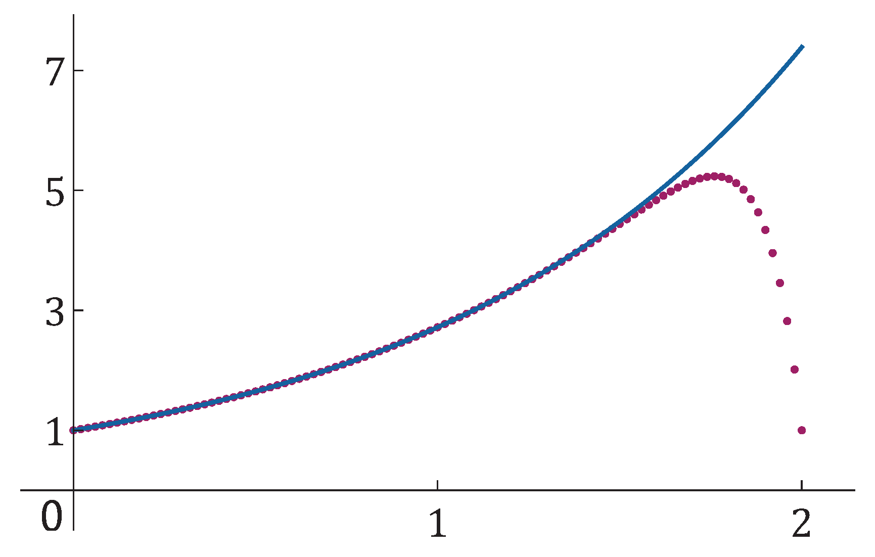
The experimental results in Table 3 show that the error of the numerical method is less than . The results in Table 3 represent a significant improvement over those in Table 3 for the numerical method (16). The graphs of the exact solution of equation (17) on the interval and numerical solution are given in Figure 3.
Figure 1.
Graphs of the exact solution of equation (17) and of the numerical solution for and .
Figure 1.
Graphs of the exact solution of equation (17) and of the numerical solution for and .
Example 3.
Consider the ordinary differential equation
for , and the corresponding boundary value ordinary differential equation
where
□
Equation (26) has a solution . The numerical solution of the initial value ordinary differential equation
which uses 2-point approximation (24) is computed as
The numerical solution of the boundary value ordinary differential equation
which uses two-point approximation (24) is computed as
Denote by the numerical solution (28) of equation (26), and by the first half of the values of (29), regarded as a numerical solution of equation (26). The second column of Table 4 contains the numerical results for the error and order of numerical solution . The third and fourth columns contain the results for the error and order of numerical solution .
The graphs of the solution of equation (26) and numerical solution (29) of boundary value ordinary differential equation (27) are given on Figure 2. While the numerical results in the second column of Table 4 show that the numerical solution is of first order, its error is quite large, making this method impractical for real applications. The applied approach for computing the numerical solutions of the ordinary differential equations (17) and (26), which uses the numerical solutions of the boundary value problems (25) and (27), allows one to obtain solutions with an error smaller than , which is sufficient for real-life problems.
Shifted approximations are employed for the solution of nonlinear ordinary differential equations. In order to derive the shifted approximation of (11), we make use of the two-point approximation (24).
When we obtain
From (11) and (30) we obtain the shifted approximation of the first derivative
Consider the nonlinear ordinary differential equation
By approximating the first derivative at with (31) we obtain
The numerical solution of equation (32) satisfies
and has initial conditions
The numerical solution (33) is computed with operations. The number of computations can be reduced to in the following way [1]: Let
The sequence is computed recursively as
The sequence and the numerical solution (33) are computed with operations by means of the following pseudocode.
Initialization:
Loop: for n from 3 to N do
The computational time of the numerical method (33) is comparable to that of standard difference methods. The numerical solution (33) has first-order accuracy, and second-order accuracy when . When the parameter , the numerical solution (33) has an accuracy of order .
Example 4.
Consider the following nonlinear ordinary differential equation
4. Second-Order Approximations of the Fractional Derivative
In this section, we derive the second-order expansion formula for the L1 approximation. Second-order approximations of the fractional derivative, whose weights satisfy properties (2), are constructed using the expansion formula and the approximation (11) of the second derivative.
4.1. Second Order Expansion Formula
In the next claim, we express the L1 approximation in terms of the values of the second derivative.
Claim 8.
Let . Then
where
Proof.
By rearranging the terms, the formula of the L1 approximation can be written in the form
The central difference approximation of the second derivative is given by
where . Then
From the formula for the sum of zeta sequence
Therefore
The error of (35) satisfies
□
Let , where and . Denote
The trapezoidal rule of the function G on the interval is defined as:
Claim 9.
Let . Then
where
Proof.
The function G has first and second derivatives
From the Mean Value Theorem
where . Hence
The error of the trapezoidal rule satisfies
where is the second Bernoulli polynomial
The polynomial satisfies for . Therefore
because . The first derivative has a value at zero
where , which implies that
The coefficient of the trapezoidal approximation error satisfies the estimate
□
Let
Claim 10.
Let . Then
Proof.
From Taylor’s theorem
where . Therefore
□
By integrating by parts the formula in the definition of Caputo derivative we find
In the following theorem, we obtain the second-order expansion formula of the L1 approximation and derive an error estimate.
Theorem 11.
Let . Then
where
Proof.
By adding and subtracting in (37) we get
From Claim 9 and Claim 10 the trapezoidal rule for the function
has a second order accuracy
where
From Claim 8
where ,
Therefore
From Taylor’s theorem
where
L1 approximation has a second-order expansion formula
where
and
□
Corollary 12.
Let . Then
where
Proof.
By approximating the second derivative in the expansion formula (38) of the L1 approximation with we obtain a second order approximation of the fractional derivative
where
By substituting with the value of the zeta function we obtain a second order asymptotic approximation of the fractional derivative
where
The errors of approximations (39) and (40) satisfy the following estimates.
Corollary 13.
Let . Then
where and
Proof.
The zeta function is decreasing on and takes values between and . Therefore
The estimates for and follow from Claim 1, Theorem 11 and Corollary 12. □
4.2. Properties of the Approximations
Now we prove that, when the parameter , the weights of of approximations (39) and (40) satisfy properties (2). The values and are negative, while the weights and are positive; and are negative. In the following we show that the remaining weights and are negative. The proof relies on the inequalities from the claims below.
Claim 14.
Let . Then
Proof.
Let . Then
The function f has a maximum when .
□
Claim 15.
Let . Then
Proof.
The function g is positive because it is increasing and . □
Lemma 16.
Let . Then
Proof.
When , approximation (40) has weights
The zeta function is decreasing on and . It is sufficient to prove that
Let . From Mean Value Theorem
for some . Therefore
Inequality (41) follows from
From Claim 14
It is sufficient to prove that
Substitute .
When , the parameter , because . Then and . From Claim 15
The function is increasing, because
The function g has a maximum at .
□
From the properties of the L1-approximation and the constructions of (39) and (40), their weights satisfy . Therefore, approximation (40) satisfies properties (2). The weights of approximation (39) also satisfy the properties in (2), since . In the following claim, we establish a lower bound for the last weight of both approximations.
Claim 17.
Proof.
From the binomial formula
The values of are negative. Hence
□
4.3. Shifted Approximations for the Fractional Derivative
Now we derive shifted approximations of the fractional derivative on the first two-point and three-point stencils of the uniform mesh. These shifted approximations are used to specify the initial conditions in the numerical solutions of fractional differential equations that employ approximations (39) and (40) of the fractional derivative. From Taylor’s theorem
By substituting the first derivative in the definition of the Caputo fractional derivative (1) with the second Taylor polynomial, we obtain
Substitute .
Now we obtain a shifted approximation of the fractional derivative on the two-point stencil from the approximation
where . Let
The function has a Taylor expansion of order two at the origin; that is,
By setting the coefficients equal to zero, we obtain the system of equations
The system of equations has a solution
From Taylor’s theorem and the values of the coefficients given above, we obtain
where . Therefore
where
A shifted approximation on the three-point stencil is obtained from (42) for .
where . Let
The function has a Taylor expansion of order two at the origin; that is,
By setting the coefficients equal to zero, we obtain the system of equations
which has a solution
From Taylor’s theorem and the values of the coefficients given above, we obtain
where
Hence
where
5. Numerical Solutions of Fractional Differential Equations
Difference schemes are the main approach for the numerical solution of ordinary and partial fractional differential equations [52,53,54,55,56,57,58]. In paper [1], we construct difference schemes for the two-term ordinary fractional differential equation and the fractional subdiffusion equation, which use approximations of the fractional derivative of order , obtained in a manner similar to the construction of approximations (6) and (8). In this section, we study the difference schemes that use approximations (6) and (8). The convergence and order of the difference schemes based on the second-order asymptotic approximation (8) are proved. Consider the two-term ordinary fractional differential equation
Suppose that
is an approximation of the fractional derivative that has an error term . By substituting the fractional derivative in equation (45) with (46), we obtain
The numerical solution of equation (45) obtained using approximation (46) is computed as
The initial values of and are computed using the L1 approximation, where for . Denote by the numerical solution (47) of equation (45) that uses approximation (6), where , and by the numerical solution that uses approximation (8), where .
Example 5.
Consider the following boundary value OFDE
Equation (48) has a solution . The numerical results for the error and order of numerical solutions and on the interval are given in Table 6 and Table 7. The error of numerical solution is smaller than the error of because approximation (6) has a smaller truncation error than (8). The computational time of is longer that that of because on every iteration the weights of approximation (6) are recomputed.
In the following, we prove the convergence of the numerical solution and obtain an estimate for the error. Denote by the error of at the point . The errors and are computed as and
where is the truncation error of the L1 approximation [48]. Therefore, the numerical solution has second-order accuracy for the first four iterations. Let
The sequence of the errors of numerical solution , for satisfies
Theorem 18.
Suppose that . Then
where and
Proof.
We prove the statement by induction on n. The estimate holds for . Assume that (49) holds for all .
Applying the induction assumption
From Corollary 13 and Claim 17
Factoring out we write
When , the number . Hence
To ensure , it suffices to show that the coefficient is at most one:
From Corollary 13 and , we obtain
Combining (50) with the bound for A, we obtain that when
estimate (49) holds, , completing the induction. □
In Theorem 18, we proved that when the parameter numerical solution has second-order accuracy. The proof of the convergence and order of is similar. When the parameter L is negative, the errors of the two numerical solutions become large. Experimental results for the error and order of and for negative values of the parameter L are presented in Table 8 and Table 9. The errors of the numerical solutions in Table 8 and Table 9 are greater than for , , and .
The numerical methods and exhibit behavior similar to that of numerical method (16) for equation (14) To compute the numerical solution of equation (48) with an accuracy not exceeding , we use the approach from Example 2. We consider the corresponding boundary value fractional ordinary differential equation whose boundary condition coincides with the initial condition of equation (48). Its numerical solution, obtained using the L1 approximation of the fractional derivative, is used as the numerical solution of equation (48), and it has an accuracy of , which is sufficient to solve both equations with an error smaller than . The accuracy of the numerical solution can be improved by using higher-order approximations of the fractional derivative and boundary conditions at different points.
Example 6.
Consider the following boundary value OFDE
Let . By approximating the fractional derivative using the L1 approximation we obtain
The numerical solution satisfies
where . The numerical solution is computed with the system of equations, which consists of equations (52) and the boundary condition . The coefficient matrix of the system has entries on the diagonal above the main diagonal and is reduced to a lower-triangular form, using row operations. The graphs of the exact solution of equation (48) and numerical solution (52) for are given on Figure 3. The experimental results for the error of the numerical solution (52) are presented in Table 10, where all errors are smaller than . The results in Table 8, Table 9, and Table 10 demonstrate that the numerical method (52) for equation (48) represents a significant improvement over and for negative values of the parameter L.
The fractional subdiffusion equation is a fractional partial differential equation of the following form
where L is the diffusion coefficient and has initial and boundary conditions
Let and , where M and N are integers. Denote and by the rectangular grid on
By substituting the fractional derivative at the point with approximation (8) and the second-order partial derivative with the second-order central difference formula, we obtain
where and are the coefficients of the error of approximation (8) and is the error of central difference approximation. Denote .
The numerical solution on row m of the grid is computed as
where and has boundary conditions .
The numerical solution for the first row is obtained using shifted approximation (43)
Let . The numerical solution satisfies
and has boundary conditions boundary conditions . The coefficient matrix for the system of equations of the first row is a diagonally dominant matrix of size . The (maximum) norm of a vector is the maximum of the absolute values of its elements and the norm of a matrix is the maximum of the absolute row sums. The norm of the inverse coefficient matrix of (54) is smaller than one [49,50]. Therefore, the numerical solution on the first row of the grid has an error of order . The numerical solution for the second row of the grid is computed explicitly using the shifted approximation (44)
The numerical solution satisfies
The error of the numerical solution in the second row of is also of order . The numerical solutions for the third and fourth rows are computed explicitly using the third order approximations
The errors for the third and fourth rows also have accuracy of .
Example 7.
Consider the following fractional subdiffusion equation
Equation (55) has the solution
The numerical results for the error and order of the difference scheme (53) for the subdiffusion equation (55) with and are presented in the third and fourth columns of Table 11. The graphs for , , , and are shown in Figure 4.
Example 8.
Consider the following fractional subdiffusion equation
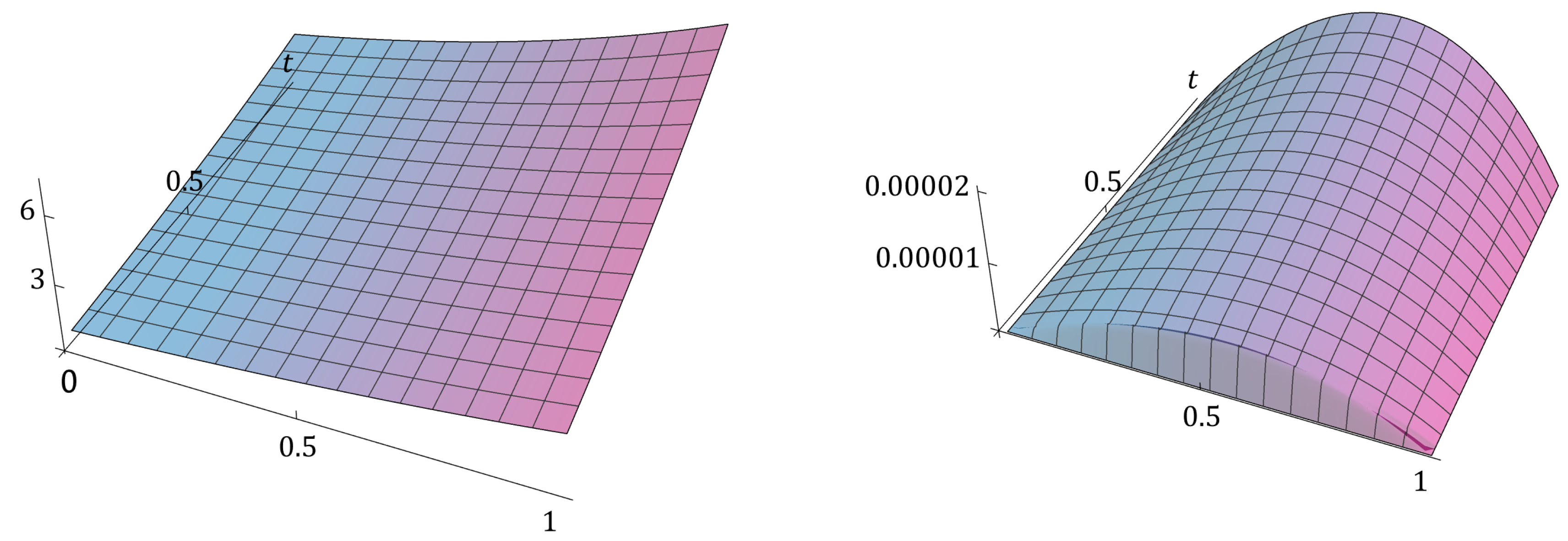
Equation (56) has the solution . The results of the numerical experiments for the error and order of the difference scheme (53) for the subdiffusion equation (56) with are presented in the second column of Table 11. The graphs of numerical solution (53) and its error for , , , and are shown in Figure 5.
In the following, we prove that the difference scheme (53) for the fractional subdiffusion equation converges with second-order accuracy. The errors on the first four rows of the grid have accuracy of . Therefore
where is a positive constant. The errors on row of the grid are the solutions of the system of equations
where and
Denote
where the maximums are taken for all and the coefficients and satisfy the bounds
Let be an -dimensional vector whose entries are the errors of difference scheme (53) on row m of the grid , and let be the vector of truncation errors (57). The system of equations for the errors of difference scheme (53) in row m of the grid can be written in matrix form as
where is a tridiagonal square matrix with nonzero entries and
Theorem 19.
The errors of difference scheme (53) satisfy
for all , where
Proof.
We prove the statement by induction. The estimate (59) holds for . Assume that (59) holds for all rows of the grid . From formula (57)
When the gamma function satisfies (see [51]). Applying the induction assumption
where . From Claim 17
When C satisfies the conditions of the theorem, the two coefficients and are positive.Therefore
From (58) the infinity norm of the inverse matrix satisfies [49,50]
Hence
The error estimate (59) holds for the m-th row of the grid , completing the induction. □
6. Conclusions
In the present paper, we have studied the construction and properties of parameter-dependent approximations for the first and second derivatives, denoted by (4), (5), and for the Caputo fractional derivative, denoted by (6) and (8) and their applications for numerical solution of differential and fractional differential equations. The approximations of the fractional derivative are developed using the second-order expansion formula of the L1 approximation together with an approximation (5) of the second derivative. The weights of the two obtained approximations of the fractional derivative satisfy property (2) when the parameter takes the value , where is the order of the fractional derivative. Approximation (6) of the fractional derivative has second-order accuracy, while the order of approximation (8) depends on the mesh size and increases from to 2. We provide examples demonstrating the application of the derived approximations to the construction of finite difference schemes for the numerical solution of fractional differential equations, and we analyze the convergence and order of these numerical solutions. In Theorem 18 and Theorem 19, we prove that the difference schemes based on both approximations (6) and (8) achieve second-order accuracy. The proofs rely on the properties (2) of the approximation weights and on the magnitude of the last weights. The theoretical results for the order and accuracy of the proposed numerical methods are confirmed by the presented numerical experiments.
In future work, we will continue the investigations initiated in this paper. We plan to address questions related to high-order expansion formulas and to the construction of approximations of the fractional derivative based on these formulas. We will also consider the development of high-order finite difference schemes for the numerical solution of fractional differential equations and analyze their performance and convergence.
Author Contributions
Conceptualization, Y.D. and S.G.; data curation, V.T.; formal analysis, Y.D. and R.M.; funding acquisition, S.G.; investigation, Y.D. and V.T.; methodology, V.T. and R.M.; project administration, S.G. and V.T.; resources, R.M.; software, S.G. and R.M.; supervision, Y.D.; validation, V.T.; visualization, S.G.; writing—original draft, Y.D. and S.G.; writing—review and editing, R.M. and V.T. All authors have read and agreed to the published version of the manuscript.
Funding
This study was supported by project BG16RFPR002-1.014-0004 UNITe, funded by the Programme “Research, Innovation and Digitalisation for Smart Transformation”, co-funded by the European Union.
Data Availability Statement
The data presented in this study are available on request from the corresponding author.
Conflicts of Interest
The authors declare no conflict of interest.
References
- Dimitrov, Y.; Georgiev, S.; Todorov, V. First Derivative Approximations and Applications. Fractal Fract. 2024, 8, 608. [Google Scholar] [CrossRef]
- Chawla, S.; Urmil; Singh, J. A Parameter-Robust Convergence Scheme for a Coupled System of Singularly Perturbed First Order Differential Equations with Discontinuous Source Term. Int. J. Appl. Comput. Math 2021, 7, 118. [CrossRef]
- Riaz, M.B.; Saeed, S.T.; Baleanu, D.; Ghalib, M.M. Computational Results with Non-Singular and Non-Local Kernel Flow of Viscous Fluid in Vertical Permeable Medium with Variant Temperature. Front. Phys. 2020, 8, 275. [Google Scholar] [CrossRef]
- Srivastava, H.M.; Adel, W.; Izadi, M.; El-Sayed, A.A. Solving Some Physics Problems Involving Fractional-Order Differential Equations with the Morgan–Voyce Polynomials. Fractal Fract. 2023, 7, 301. [Google Scholar] [CrossRef]
- Ghanbari, B.; Atangana, A. A New Application of Fractional Atangana–Baleanu Derivatives: Designing ABC-Fractional Masks in Image Processing. Physica A 2020, 542, 123516. [Google Scholar] [CrossRef]
- Sabri, T.M.T.; Abdo, M.S.; Shah, K.; Abdeljawad, T. Study of Transmission Dynamics of COVID-19 Mathematical Model under ABC Fractional Order Derivative. Results Phys. 2020, 19, 103507. [Google Scholar] [CrossRef]
- Alqahtani, A.M.; Sharma, S.; Chaudhary, A.; Sharma, A. Application of Caputo–Fabrizio Derivative in Circuit Realization. AIMS Math. 2025, 10, 2415–2443. [Google Scholar] [CrossRef]
- Sun, Z.Z.; Gao, G. Fractional Differential Equations: Finite Difference Methods; De Gruyter: Berlin, Germany, 2020; ISBN 978-3-11-061606-4. [Google Scholar]
- Arshad, S.; Baleanu, D.; Huang, J.; Al Qurashi, M.M.; Tang, Y.; Zhao, Y. Finite Difference Method for Time-Space Fractional Advection–Diffusion Equations with Riesz Derivative. Entropy 2018, 20, 321. [Google Scholar] [CrossRef]
- Li, C.; Zeng, F. Finite Difference Methods for Fractional Differential Equations. Int. J. Bifurc. Chaos 2012, 22, 1230014. [Google Scholar] [CrossRef]
- Podlubny, I. Fractional Differential Equations; Academic Press: San Diego, CA, USA, 1999. [Google Scholar]
- Zayernouri, M.; Wang, L.-L.; Shen, J.; Karniadakis, G.E. Spectral and Spectral Element Methods for Fractional Ordinary and Partial Differential Equations; Cambridge University Press: Cambridge, UK, 2024. [Google Scholar]
- Shi, X.; Zhou, D.-X. Spectral Collocation Methods for Fractional Integro-Differential Equations with Weakly Singular Kernels. J. Sci. Comput. 2023, 94, 112. [Google Scholar] [CrossRef]
- Papadopoulos, I.P.A.; Olver, S. A Sparse Spectral Method for Fractional Differential Equations in One-Spatial Dimension. Adv. Comput. Math. 2024, 50, 69. [Google Scholar] [CrossRef]
- Shu, D.; Jia, X. High Accuracy Spectral Method for the Space-Fractional Diffusion Equations. J. Math. Study 2014, 47, 274–286. [Google Scholar] [CrossRef]
- J. Gao, M. Zhao, N. Du, X. Guo, H. Wang, and J. Zhang. A finite element method for space–time directional fractional diffusion partial differential equations in the plane and its error analysis. J. Comput. Appl. Math. 2019, 362, 354–365. [CrossRef]
- Ford, N.J.; Xiao, J.; Yan, Y. A Finite Element Method for Time Fractional Partial Differential Equations. Fract. Calc. Appl. Anal. 2011, 14, 454–474. [Google Scholar] [CrossRef]
- Su, X.; Zhou, Y. A Fast High-Order Predictor–Corrector Method on Graded Meshes for Solving Fractional Differential Equations. Fractal Fract. 2022, 6, 516. [Google Scholar] [CrossRef]
- Sivalingam, S.M.; Kumar, P.; Trinh, H.; Govindaraj, V. A Novel L1-Predictor-Corrector Method for the Numerical Solution of the Generalized-Caputo Type Fractional Differential Equations. Math. Comput. Simul. 2024, 220, 462–480. [Google Scholar] [CrossRef]
- Jiang, S.D.; Zhang, J.W.; Zhang, Q.; Zhang, Z.M. Fast Evaluation of the Caputo Fractional Derivative and Its Applications to Fractional Diffusion Equations. Commun. Comput. Phys. 2017, 21, 650–678. [Google Scholar] [CrossRef]
- Yan, Y.G.; Sun, Z.Z.; Zhang, J.W. Fast Evaluation of the Caputo Fractional Derivative and Its Applications to Fractional Diffusion Equations: A Second-Order Scheme. Commun. Comput. Phys. 2017, 22, 1028–1048. [Google Scholar] [CrossRef]
- Li, X.; Liao, H.L.; Zhang, L.M. A Second-Order Fast Compact Scheme with Unequal Time-Steps for Subdiffusion Problems. Numer. Algorithms 2021, 86, 1011–1039. [Google Scholar] [CrossRef]
- Jiang, H.; Xu, D. A Fast High-Order Compact Difference Scheme for Time-Fractional KS Equation with the Generalized Burgers’ Type Nonlinearity. Fractal Fract. 2025, 9, 218. [Google Scholar] [CrossRef]
- Alikhanov, A.A.; Huang, C. A high-order L2 type difference scheme for the time fractional diffusion equation. Appl. Math. Comput. 2021, 411, 1–19. [Google Scholar] [CrossRef]
- Wang, Y.-M.; Ren, L. A high-order L2-compact difference method for Caputo-type time fractional sub-diffusion equations with variable coefficients. Appl. Math. Comput. 2019, 342, 71–93. [Google Scholar] [CrossRef]
- Arshad, S.; Defterli, O.; Baleanu, D. A Second Order Accurate Approximation for Fractional Derivatives with Singular and Non-Singular Kernel Applied to a HIV Model. Appl. Math. Comput. 2020, 374, 125061. [Google Scholar] [CrossRef]
- Zhang, Y.; Feng, X.; Qian, L. A High-Order Compact ADI Scheme for Two-Dimensional Nonlinear Schrödinger Equation with Time Fractional Derivative. Comput. Appl. Math. 2025, 44, 168. [Google Scholar] [CrossRef]
- Feng, Y.; Zhang, X.; Chen, Y.; Wei, L. A compact finite difference scheme for solving fractional Black-Scholes option pricing model. J. Inequal. Appl. 2025, 2025, 36. [Google Scholar] [CrossRef]
- Cao, J.; Cai, Z. Numerical analysis of a high-order scheme for nonlinear fractional differential equations with uniform accuracy. Numer. Math. Theory Methods Appl. 2020, 14, 71–112. [Google Scholar] [CrossRef]
- Dehghan, M.; Safarpoor, M.; Abbaszadeh, M. Two high-order numerical algorithms for solving the multi-term time fractional diffusion-wave equations. J. Comput. Appl. Math. 2015, 290, 174–195. [Google Scholar] [CrossRef]
- Roul, P.; Rohil, V. A novel high-order numerical scheme and its analysis for the two-dimensional time fractional reaction-subdiffusion equation. Numer. Algor. 2022, 90, 1357–1387. [Google Scholar] [CrossRef]
- Hao, Z.-P.; Sun, Z.-Z.; Cao, W.-R. A fourth-order approximation of fractional derivatives with its applications. J. Comput. Phys. 2015, 281, 787–805. [Google Scholar] [CrossRef]
- Tian, J.; Ding, H. Improved High-Order Difference Scheme for the Conservation of Mass and Energy in the Two-Dimensional Spatial Fractional Schrödinger Equation. Fractal Fract. 2025, 9, 280. [Google Scholar] [CrossRef]
- Shams, M.; Carpentieri, B. Efficient families of higher-order Caputo-type numerical schemes for solving fractional order differential equations. Alexandria Eng. J. 2025, 124, 337–361. [Google Scholar] [CrossRef]
- Lubich, C. Discretized fractional calculus. SIAM J. Math. Anal. 1986, 17, 704–719. [Google Scholar] [CrossRef]
- Dimitrov, Y.; Miryanov, R.; Todorov, V. Asymptotic Expansions and Approximations for the Caputo Derivative. Comput. Appl. Math. 2018, 37, 5476–5499. [Google Scholar] [CrossRef]
- Jin, B.; Lazarov, R.; Zhou, Z. An analysis of the L1 scheme for the subdiffusion equation with nonsmooth data. IMA J. Numer. Anal. 2016, 36, 197–221. [Google Scholar] [CrossRef]
- Li, B.; Xie, X.; Yan, Y. L1 scheme for solving an inverse problem subject to a fractional diffusion equation. Comput. Math. Appl. 2023, 134, 112–123. [Google Scholar] [CrossRef]
- Scherer, R.; Kalla, S.L.; Tang, Y.; Huang, J. The Grünwald–Letnikov method for fractional differential equations. Comput. Math. Appl. 2011, 62(3), 902–917. [Google Scholar] [CrossRef]
- Todorov, V.; Dimitrov, Y.; Dimov, I. Second order shifted approximations for the first derivative. In: Dimov I., Fidanova S. (eds) Advances in High Performance Computing. HPC 2019. Studies in Computational Intelligence 2011, 902, Springer, Cham. [Google Scholar] [CrossRef]
- Apostolov, S.; Dimitrov, Y.; Todorov, V. Constructions of second order approximations of the Caputo fractional derivative. In: Lirkov I., Margenov S. (eds) Large-Scale Scientific Computing. LSSC 2021. Lecture Notes in Computer Science, Springer, 2022, 13127. [CrossRef]
- Al-khawaldeh, H.O.; Batiha, I.M.; Zuriqat, M.; Anakira, N.; Ogilat, O.; Sasa, T. A numerical approach for solving fractional linear boundary value problems using shooting method. J. Math. Anal. 2025, 16, 1–20. [Google Scholar] [CrossRef]
- Bakodah, H.O.; Alzahrani, K.A.; Alzaid, N.A.; Almazmumy, M.H. Efficient decomposition shooting method for tackling two-point boundary value models. J. Umm Al-Qura Univ. Appl. Sci. 2025, 11, 319–329. [Google Scholar] [CrossRef]
- Alzaid, N.; Alzahrani, K.; Bakodah, H. A modification of the efficient decomposition shooting method for two-point boundary-value problems. Contemp. Math. 2025, 6, 3400–3416. [Google Scholar] [CrossRef]
- Filipov, S.M.; Gospodinov, I.D.; Faragó, I. Shooting-projection method for two-point boundary value problems. Appl. Math. Lett. 2017, 72, 10–15. [Google Scholar] [CrossRef]
- Georgiev, S.G.; Vulkov, L.G. Numerical determination of the right boundary condition for regime–switching models of European options from point observations. AIP Conf. Proc. 2018, 2048, 030003. [Google Scholar] [CrossRef]
- Butcher, J.C. Numerical Methods for Ordinary Differential Equations, 3rd ed.; Wiley: Chichester, UK, 2016. [Google Scholar]
- Cai, M.; Li, C. Numerical Approaches to Fractional Integrals and Derivatives: A Review. Mathematics 2020, 8, 43. [Google Scholar] [CrossRef]
- Kolotilina, L.Y. Bounds for the infinity norm of the inverse for certain M- and H-matrices. Linear Algebra Appl. 2009, 430, 692–702. [Google Scholar] [CrossRef]
- Varah, J.M. A lower bound for the smallest singular value of a matrix. Linear Algebra Appl. 1975, 11(1), 3–5. [Google Scholar] [CrossRef]
- Deming, W.; Colcord, C. The minimum in the gamma function. Nature 1935, 135, 917. [Google Scholar] [CrossRef]
- Cao, J.; Xu, C. A high order scheme for the numerical solution of the fractional ordinary differential equations. J. Comput. Phys. 2013, 238, 154–168. [Google Scholar] [CrossRef]
- Gülsu, M.; Öztürk, Y.; Anapalı, A. Numerical approach for solving fractional relaxation-oscillation equation. Appl. Math. Model. 2013, 37, 5927–5937. [Google Scholar] [CrossRef]
- Diethelm, K.; Ford, J. Numerical Solution of the Bagley–Torvik Equation. BIT Numer. Math. 2002, 42, 490–507. [Google Scholar] [CrossRef]
- Ali, U.; Sohail, M.; Abdullah, F.A. An efficient numerical scheme for variable-order fractional sub-diffusion equation. Symmetry 2020, 12, 1437. [Google Scholar] [CrossRef]
- Langlands, T.A.M.; Henry, B.I. The accuracy and stability of an implicit solution method for the fractional diffusion equation. J. Comput. Phys. 2005, 205, 719–736. [Google Scholar] [CrossRef]
- Duo, S.; Ju, L.; Zhang, Y. A fast algorithm for solving the space–time fractional diffusion equation. Comput. Math. Appl. 2018, 75, 1929–1941. [Google Scholar] [CrossRef]
- Wang, H.; Basu, T.S. A Fast Finite Difference Method for Two-Dimensional Space-Fractional Diffusion Equations. SIAM J. Sci. Comput. 2012, 34, A2444–A2458. [Google Scholar] [CrossRef]
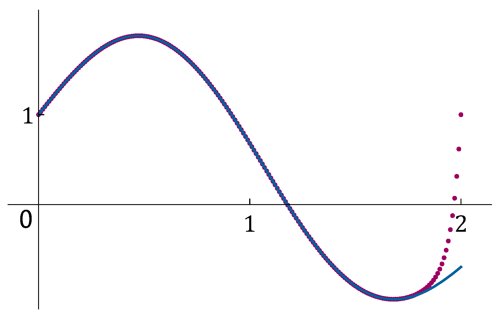
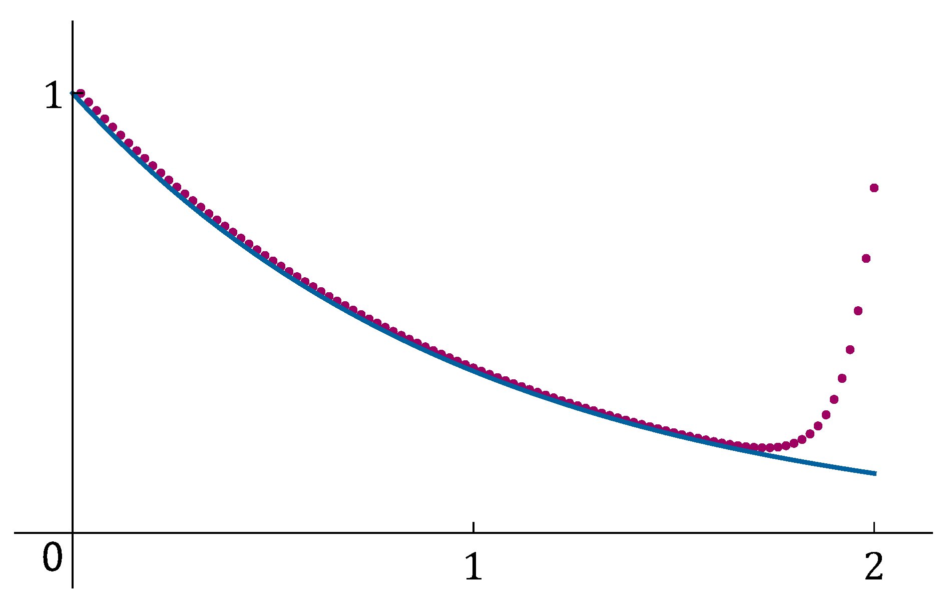
Figure 4.
Graphs of the numerical solution of equation (55) - left and the corresponding error - right for ,, , and .
Figure 4.
Graphs of the numerical solution of equation (55) - left and the corresponding error - right for ,, , and .
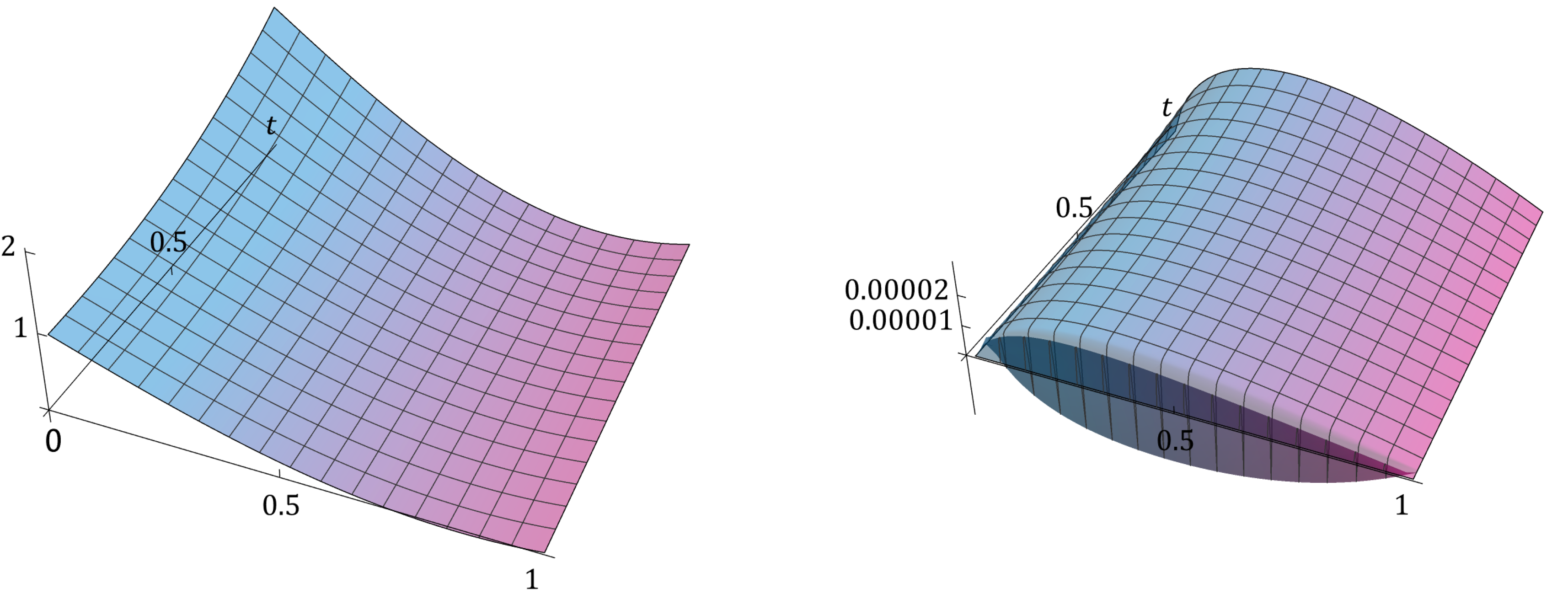
Figure 5.
Graphs of the numerical solution of equation (56) - left and the corresponding error - right for ,, , and .
Figure 5.
Graphs of the numerical solution of equation (56) - left and the corresponding error - right for ,, , and .

| Error | Order | Error | Order | Error | Order | |
|---|---|---|---|---|---|---|
| Error | Order | Error | Order | Error | Order | |
|---|---|---|---|---|---|---|
Table 3.
Error and order of numerical method of equation (17) and .
Table 3.
Error and order of numerical method of equation (17) and .
| Error | Order | Error | Order | Error | Order | |
|---|---|---|---|---|---|---|
Table 4.
Error and order of numerical solutions and of equation (26).
Table 4.
Error and order of numerical solutions and of equation (26).
| Error | Order | Error | Order | Error | Order | |
|---|---|---|---|---|---|---|
| Error | Order | Error | Order | Error | Order | |
|---|---|---|---|---|---|---|
Table 6.
Error and order of numerical solution of equation (48).
Table 6.
Error and order of numerical solution of equation (48).
| Error | Order | Error | Order | Error | Order | |
|---|---|---|---|---|---|---|
Table 7.
Error and order of numerical solution of equation (48).
Table 7.
Error and order of numerical solution of equation (48).
| Error | Order | Error | Order | Error | Order | |
|---|---|---|---|---|---|---|
Table 8.
Error and order of numerical method of equation (48).
Table 8.
Error and order of numerical method of equation (48).
| Error | Order | Error | Order | Error | Order | |
|---|---|---|---|---|---|---|
Table 9.
Error and order of numerical method of equation (48).
Table 9.
Error and order of numerical method of equation (48).
| Error | Order | Error | Order | Error | Order | |
|---|---|---|---|---|---|---|
Disclaimer/Publisher’s Note: The statements, opinions and data contained in all publications are solely those of the individual author(s) and contributor(s) and not of MDPI and/or the editor(s). MDPI and/or the editor(s) disclaim responsibility for any injury to people or property resulting from any ideas, methods, instructions or products referred to in the content. |
© 2025 by the authors. Licensee MDPI, Basel, Switzerland. This article is an open access article distributed under the terms and conditions of the Creative Commons Attribution (CC BY) license (http://creativecommons.org/licenses/by/4.0/).
Copyright: This open access article is published under a Creative Commons CC BY 4.0 license, which permit the free download, distribution, and reuse, provided that the author and preprint are cited in any reuse.


