Preprint
Article

This version is not peer-reviewed.

An Improved Real-Time Lightweight YOLOv8 Algorithm for Bloom Maturity Recognition in Torreya Grandis

Submitted:

21 January 2026

Posted:

22 January 2026

You are already at the latest version

Abstract

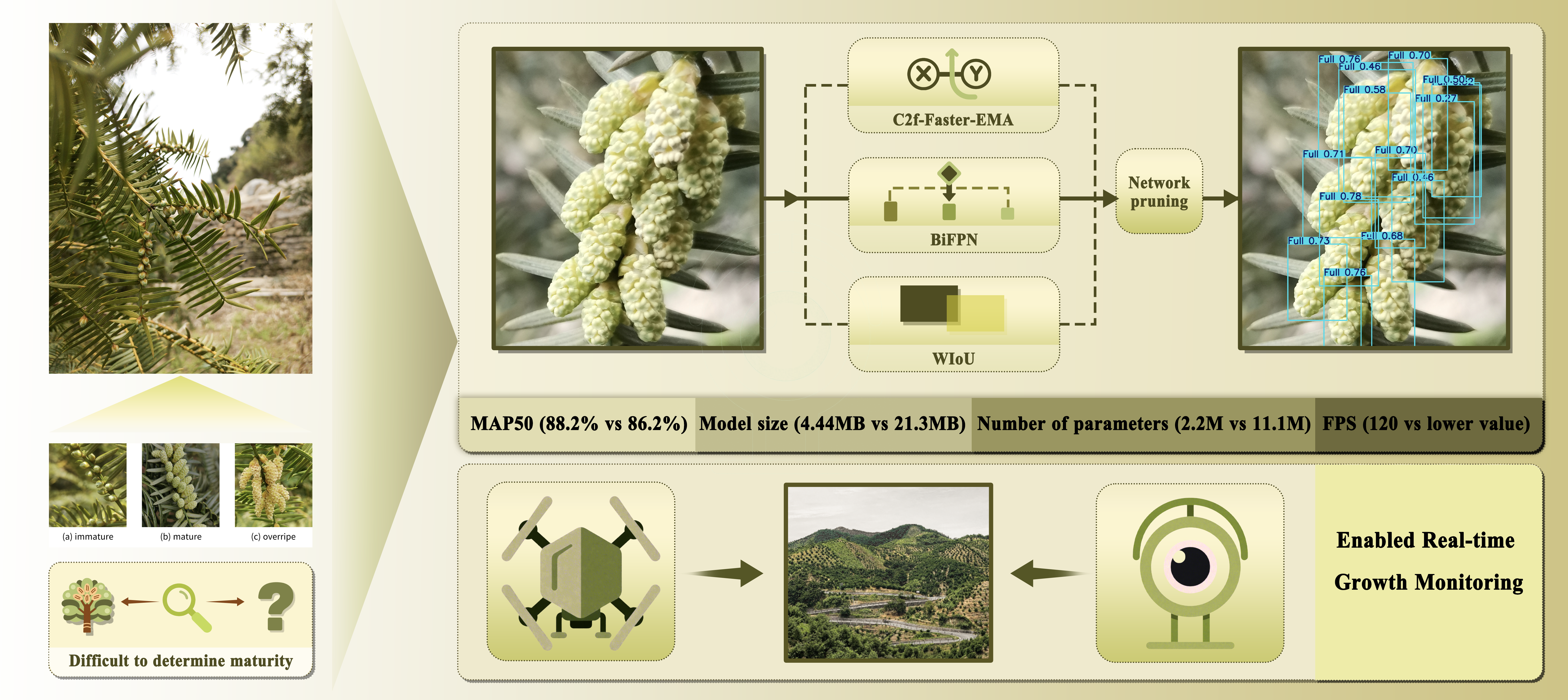
To address the challenge of rapidly and accurately detecting male cones of Chinese Torreya at various stages of maturity in natural environments, the research team proposes a target detection algorithm, GFM-YOLOV8s, based on an improved YOLOv8s. By utilizing the YOLOv8s network model as the foundation, we replace the backbone feature extraction network with c2f-faster-ema to lighten the model and simultaneously enhance its ability to capture and express important image features. Additionally, the PAN-FPN feature extraction structure in the neck is substituted with a BiFPN structure. By removing less contributive nodes and adding cross-layer connections, the algorithm achieves better fusion and utilization of features at different scales. The WIoU loss function is introduced to mitigate the mismatch in orientation between the predicted and ground truth bounding boxes. Furthermore, a structured pruning strategy was applied to the optimized network, significantly reducing redundant parameters while preserving accuracy. Results: The improved GFM-YOLOV8 has a detection accuracy of 88.2% for Torreya male cones, the detection time of a single image is 8.3 ms, and the model size is 4.44 M, fps is 120 frames, parameters is 2.20´106. Compared with the original YOLOv8s algorithm, map50 and recall are increased by 2.0% and 2.0% respectively, and the model size and model parameters are reduced by 79.2% and 80.1% respectively. The refined lightweight model can swiftly and accurately detect male cones of Torreya at different stages of maturity in natural settings, providing technical support for the visual recognition system used in growth monitoring at Torreya bases.

Keywords: 
;  ;  ;  ;  

1. Introduction

The 2020 edition of the "Chinese Pharmacopoeia" includes Torreya, a tree belonging to the genus Torreya in the Taxaceae family. Torreya has a long history of cultivation in China, with medicinal uses documented as early as the third century. This species is recognized for its high medicinal and economic value. Statistics indicate that Zhejiang Province is the largest domestic producer of Torreya, with the output from Kuaiji Mountain and its surrounding counties and cities accounting for 95% of the total Torreya production in the country. Additionally, Torreya is cultivated in other provinces, including Fujian, Jiangxi, Anhui, Hunan, and Guizhou [1]. From 2008 to 2025, the area dedicated to Torreya cultivation in Zhejiang Province has consistently expanded, leading to an increase in the fruiting area as well. Within the forestry industry of Zhejiang, Torreya holds a significant position as a specialty nut. The total planting area exceeds 1000,000 acres, with an annual output surpassing 7,000 tons and a primary output value exceeding 1.5 billion yuan, reflecting the robust development momentum of the Torreya industry. Given the substantial economic benefits associated with this sector, it is evident that the Torreya industry has the potential for broader development in the future. Key factors influencing yield include the survival rate of Torreya trees, soil quality, pollination, and pest and disease management [2,3].
The widespread application of drone pollination technology in Torreya cultivation demonstrates significant potential for ensuring high yields. However, the field currently faces two primary challenges: first, the yield and quality of Torreya male pollen cannot be consistently guaranteed, primarily due to the complexity and inefficiency of the pollen harvesting process; second, there is a lack of specific methods tailored for Torreya male trees. A real-time monitoring system for growth is particularly crucial during the critical pollination period, as the maturity status of male cones decisively influences the success rate of pollination and the final fruit yield. Notably, the pollination window for Torreya male cones is extremely narrow, and is highly susceptible to adverse weather conditions, which can severely disrupt pollen dispersal [4]. This biological constraint underscores the importance of precise timing for the harvest. During the development of male cones, initial growth is slow, followed by a rapid elongation phase that culminates in dehiscence for pollen dispersal [5]. This unique biological characteristic underscores the importance of classifying and monitoring male cone maturity to optimize pollen harvesting and improve pollination efficiency, ultimately playing a vital role in enhancing fruit yield. Therefore, the identification of Torreya male cone maturity holds significant implications for industrial development.
Traditional flower target recognition methods mainly rely on various phenotypic characteristics, such as color and shape, to identify and classify flower maturity. Liu et al. [6] conducted research on detecting tomato maturity using a machine vision algorithm based on phenotypic characteristics. They used the first-order Fourier descriptor (1D-FD) to establish an equation model for calculating the irregularity of tomato outlines and designed a classifier. The accuracy rate reached 90.7%, but the study was poor at measuring tomato maturity in the natural environment. Guo et al. [7] used a detection method based on monocular machine vision to detect lychee fruits growing under overlapping conditions, with an accuracy of 87%, but it was still unable to accurately identify targets with severe occlusion.
Traditional machine vision approaches face inherent limitations due to their heavy reliance on manually engineered features, which constrains robustness and generalization in complex agricultural environments. In contrast, deep learning—with its capacity for autonomous high-level feature extraction—has revolutionized fruit recognition and localization.
This shift in paradigm is illustrated by YOLO architectures (e.g., YOLOv3, YOLOv5, YOLOv7, YOLOv8, YOLOv10), which combine classical machine learning algorithms, computer vision libraries (OpenCV), and IoT systems to facilitate precise and efficient prediction of fruit ripening stages. Xiao et al. [8] employed CenterNet as the core network and utilized the deconvolution model DeConv to enhance the YOLOv8 model for fruit maturity detection, achieving an impressive accuracy of 99.5%. Previous research on dragon fruit [9], camellia oleifera [10], pineapple [11], strawberry [12], and jujube [13] has leveraged the robust image recognition abilities of YOLO to enable swift identification of fruit maturity.
In the agricultural field, significant progress has been made in fruit recognition using computer vision and deep learning techniques. Models based on the YOLO series demonstrate efficient and accurate performance in fruit detection, classification and maturity judgment. However, although deep learning network models exhibit powerful capabilities, their large scale and high computational cost have become a major obstacle in application scenarios with extremely high real-time requirements, such as pollen growth monitoring and mobile picking robots' visual system. Therefore, this paper proposes GFM-YOLOV8, a lightweight detection network based on an improved YOLOv8s structure. It is designed to accurately and rapidly identify the maturity stages of Torreya male cones under challenging field conditions (e.g., low light, occlusion). Through architectural enhancements and structured pruning, the model achieves a balance of accuracy and efficiency suitable for deployment on resource-constrained edge devices. This work aims to provide a practical technical solution for real-time, in-field growth monitoring, thereby supporting intelligent agricultural management.

2. Materials and Methods

2.1. Experimental Datasets

2.1.1. Datasets

This study used smartphones to collect 2648 original images of Torreya male cones under natural conditions at the Yajun Torreya base in Ancun, Lin’an District, Hangzhou City, Zhejiang Province. After selecting high-quality Torreya cultivars as the research object, we used smartphones to collect images of Torreya male bulbs every 2-3 days during the pollen growth cycle. With the aim of considering the impact of lighting on imaging, we collected images at different time periods from 8:00 to 9:00, 12:00 to 14:00, and 16:00 to 17:00, and obtained a total of 2648 original images. So as to increase the diversity of the data set and improve the robustness of the model, we expanded the data set using data enhancement methods such as changing brightness, adding salt and pepper noise, and simulating artificial occlusion, and finally obtained 4425 images.

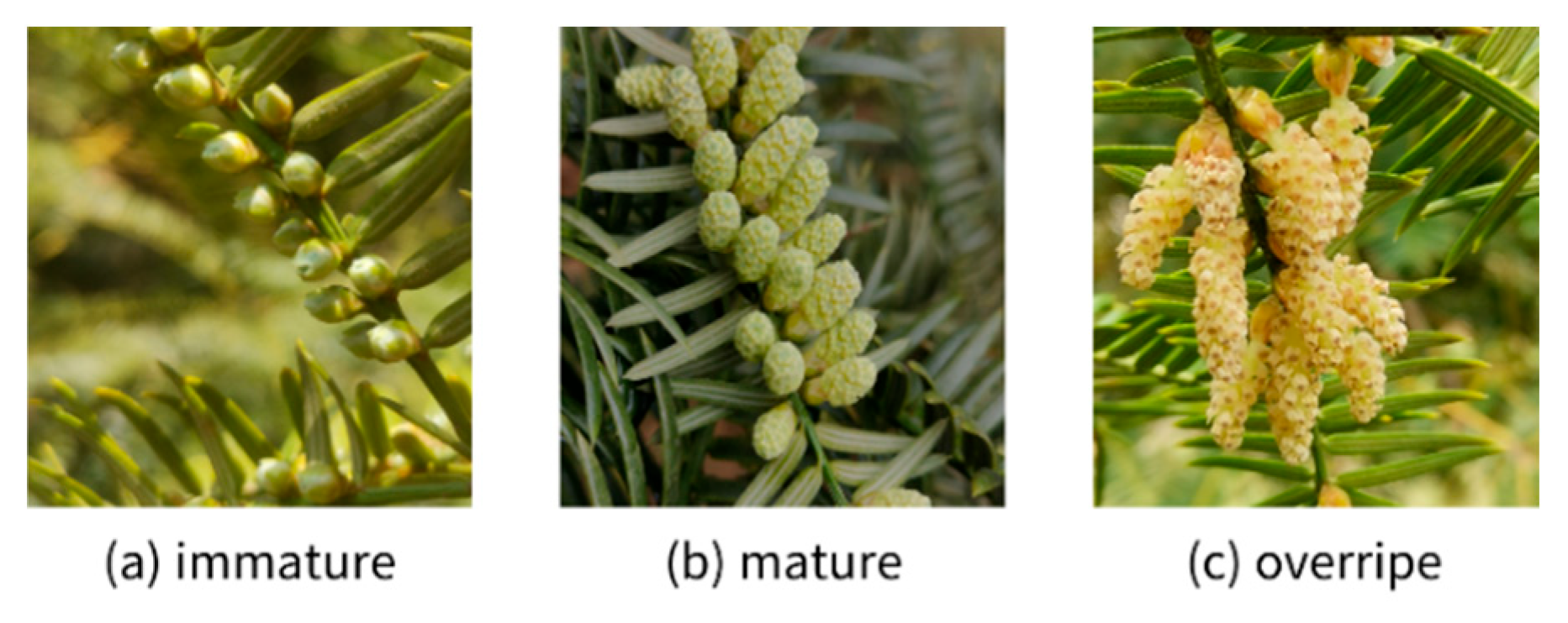
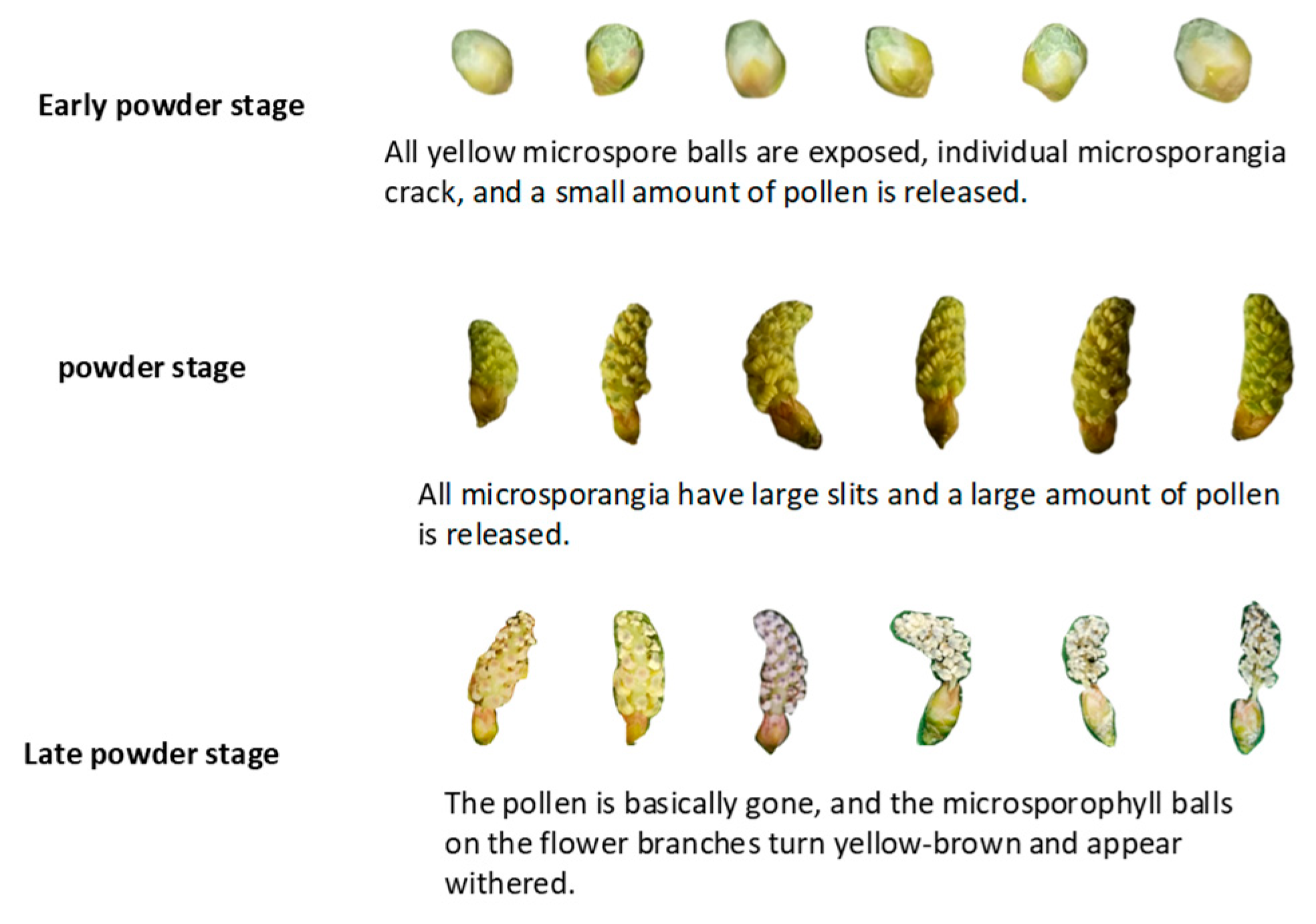
2.1.2. Classification of Maturity Levels of Torreya Male Cones

The development cycle of Torreya male cones can be subdivided into several important stages, including the flower bud stage, expansion and budding stage, discoloration stage, and mature powdering stage. In early and mid-April every year, immediately after the discoloration period, the microspores as a whole turn into bright yellow, and at the same time, the microsporophylls begin to separate from each other, followed by the dehiscence of the microsporangia. This series of changes Marks the complete maturity of pollen, followed by the loose powder stage [14]. The rupture of the microsporangium within the microspore ball means the beginning of the powdering process. This pollen period can be further divided into three periods based on the amount of pollen released. The first is the early pollen stage, when all the yellow microspore balls have been exposed, and individual microsporangia begin to crack, releasing a small amount of pollen; the next is the blooming stage, during which all the microsporangium cracks are fully opened, and a large amount of pollen is released. The pollen then disperses; the last is the late powder stage, when the pollen is almost gone, and the color of the microsporophylls on the flower branches turns to yellowish brown, showing a withered state. In addition, according to research by Torreya experts, the maturity of Torreya can be divided into three levels: immature, mature and over-ripe. With the aim of evaluating the quality of picked fruits, the physical and quality characteristics of the samples were measured, and the data were analyzed using analysis of variance and Duncan’s multiple comparison method. The third category of mature fruits has the following characteristics: 1) The immature Torreya male bulb flowers are well wrapped and not cracked, and are green. 2) The petals of mature Torreya male bulbs bloom, slightly exposed, and are yellow in color. 3) Over-mature Torreya male bulbs have obvious flower openings and pollen falls. The male bulb flowers of Torreya with different maturity levels are presented in Figure 1 and Figure 2. According to the above classification of the maturity levels of the flower bulbs of Torreya, this study tested the maturity of the male flowers of Torreya.

2.1.3. Data Generation

The original images were annotated using x-anylabels software, categorizing male cone fruits of Torreya into three classes: immature, mature, and overripe. These annotated images were partitioned into training, validation, and test sets at an 8:1:1 ratio, with detailed specifications provided in Table 1.
To ensure robust generalization capabilities of the flowering-stage maturity recognition model for Torreya grandis male cones, constructing a high-quality dataset is critical. Consequently, we performed comprehensive data augmentation on externally acquired images to further enhance model performance. Specific techniques—including geometric transformations (flipping, scaling), photometric adjustments (contrast variation), and noise injection—were applied to diversify the training data, thereby strengthening the model's adaptability.

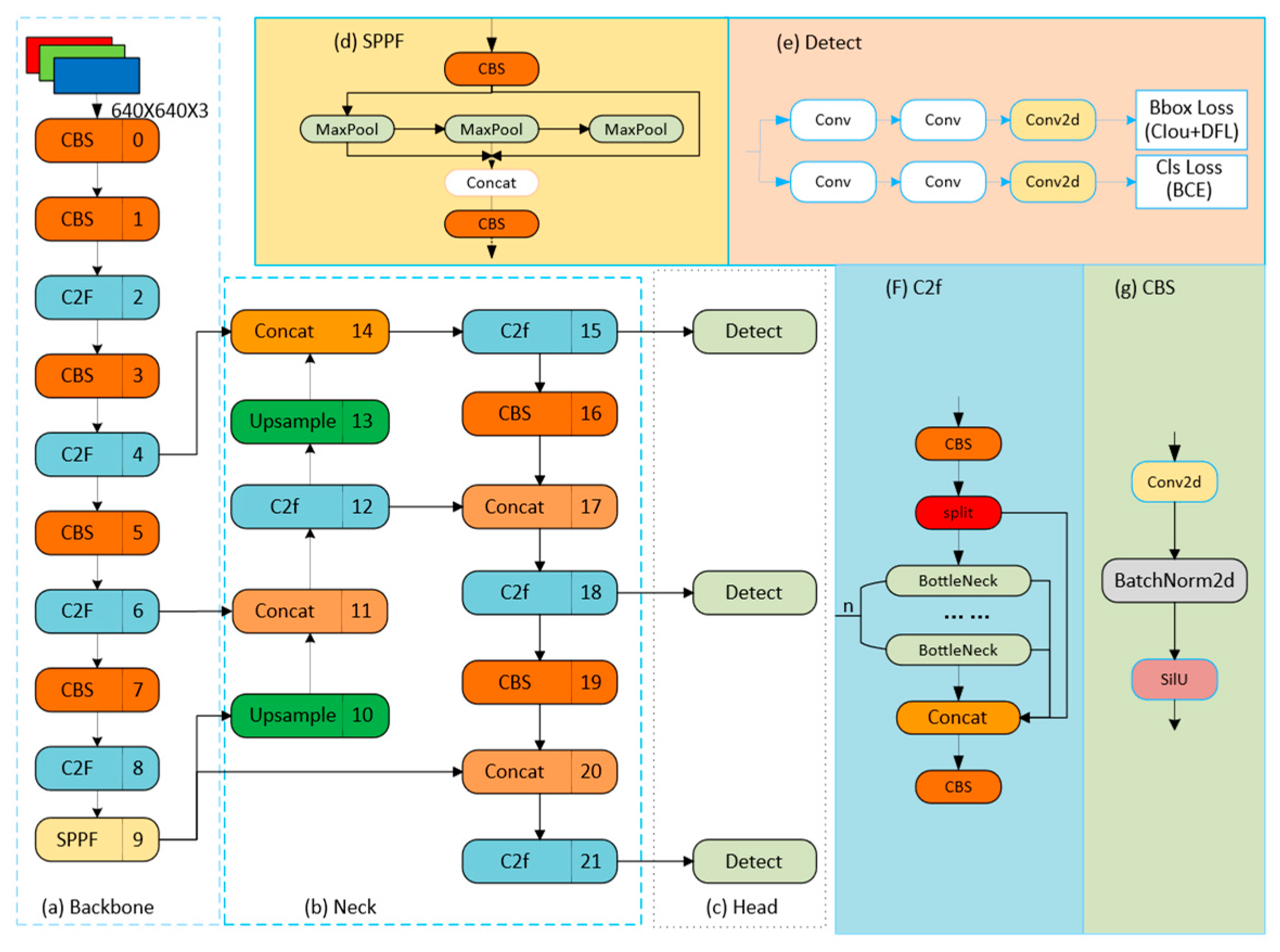
2.2. The YOLOv8 Network Architecture

Redmon et al. [15] proposed a target detection algorithm called YOLO (you only look once) in 2016. Different from the traditional R-CNN [16] series of algorithms, it does not need to extract candidate areas and directly outputs a single-stage target category and probability. detection algorithm. This algorithm has received widespread attention in the industrial and agricultural fields because of its low computational resource usage and rapid detection speed. Especially in the field of industrial target detection that requires rapid response, this feature has caused great repercussions. After years of continuous development, the latest version of the YOLO algorithm has been updated to version 11. The functions and stability of the v8 version have been recognized by the industry. Figure 3 details the specific structural configuration.
The YOLOv8 target detection algorithm is one of the newer and stable versions of the YOLO series. The overall structure mainly consists of three parts: Backbone, Neck, and Head. Its backbone network uses the CSPNet [17] structure, through the cross-connection and information integration of CSPNet. This enables the network to better transfer and integrate features at different stages, improving the feature representation ability of the model. The neck uses the path aggregation network structure PANet to generate feature maps with multi-scale information. The head uses CIOU_Loss and non-maximum suppression (NMS) to complete the output of target detection results.

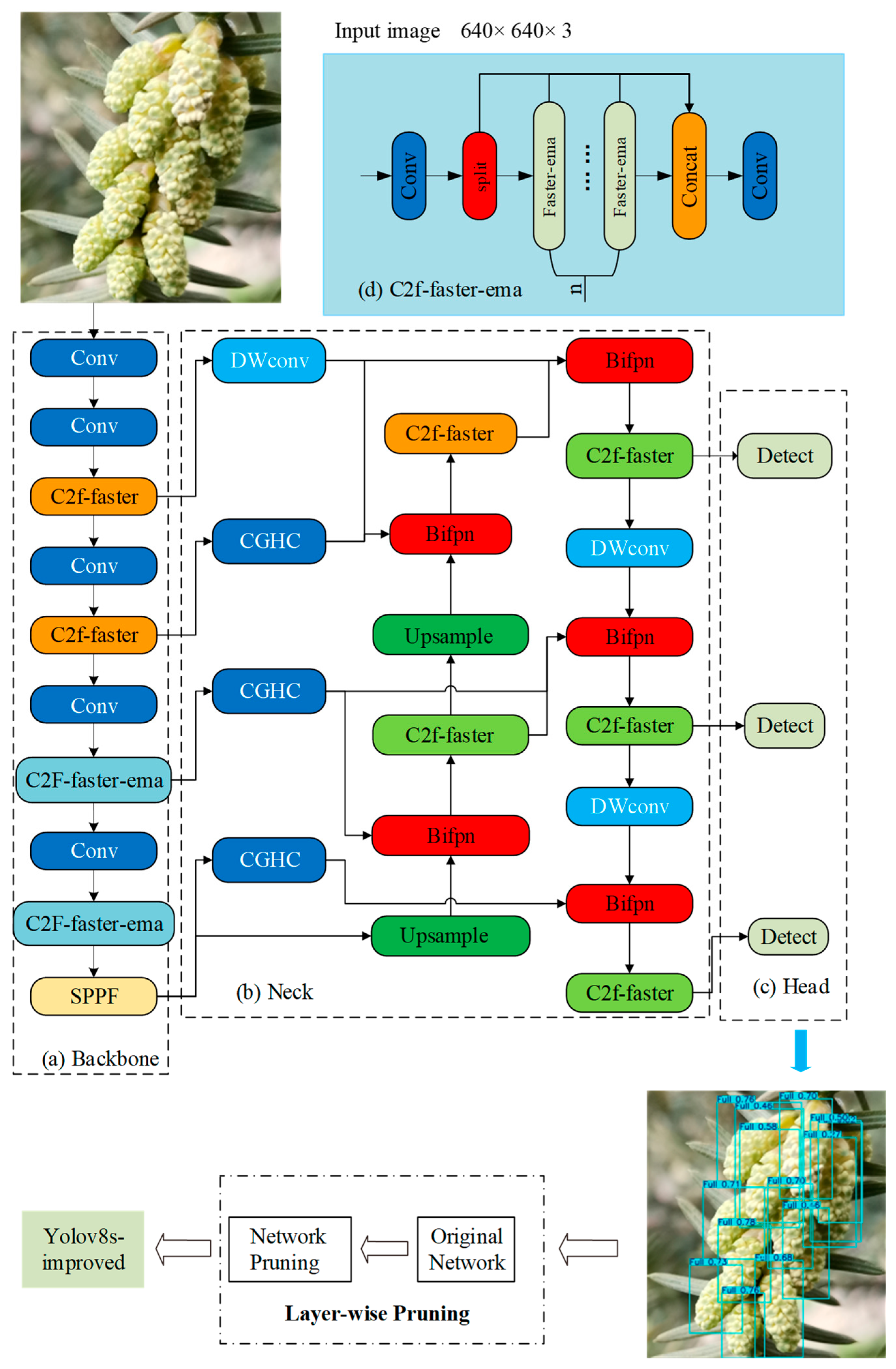
2.3. Improved Torreya Male Cone Maturity Detection Model

To achieve real-time and accurate detection in complex field conditions, we propose an enhanced architecture named GFM-YOLOv8. It integrates a C2f-Faster backbone with an EMA and a GSC-BiFPN neck (the acronym ‘GFM’ derives from these key components: GSC-BiFPN, Faster-C2F, and EMA). The overall architecture is depicted in Figure 16.
In order to optimize the YOLOv8 model, we first improved the backbone network and replaced the original complex CSPDarkNet network with a more concise and lightweight c2f-faster network, aiming to compress the model size and reduce the model depth. Subsequently, in order to improve the feature extraction and fusion capabilities of the model, especially the accuracy in detecting male cones from undehiscent to dehiscent, we introduced an efficient multi-scale attention (EMA) mechanism based on cross-space learning and combined it Integrated into c2f-faster module. By fusing shallow and deep feature maps, the model can extract richer semantic information and thus better focus on immature features. In addition, we optimized the neck structure of YOLOv8 and replaced the original PAN-FPN feature extraction structure with the more efficient BiFPN [18] structure. By removing nodes with small contributions and adding cross-layer connections, BiFPN achieves better fusion and utilization of features of different scales, which not only simplifies the feature fusion process, but also significantly reduces the parameters and calculations of the model.
In further optimization of the model, we took two key measures. On the one hand, in the neck structure, we use depthwise separable convolution (Dwconv) instead of the traditional convolution (Conv). This change effectively reduces the number of parameters of the model, thereby reducing the computational burden and improving the performance of the model. Operational efficiency. On the other hand, to enhance the regression accuracy of the model in the male cone maturity detection task, we utilize the weighted Intersection over Union (WIoU) loss function. This enables the model to make more balanced performance predictions for targets of varying sizes, ultimately improving the overall detection performance of the model.

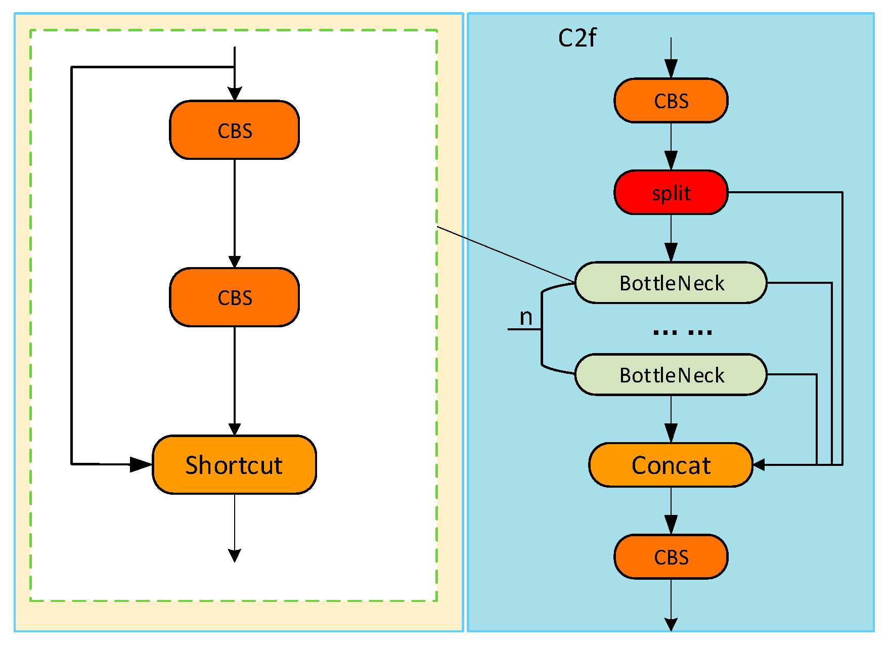
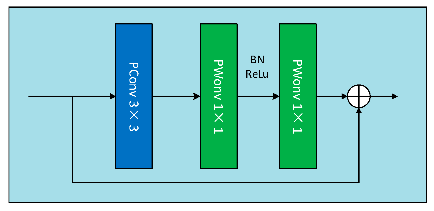
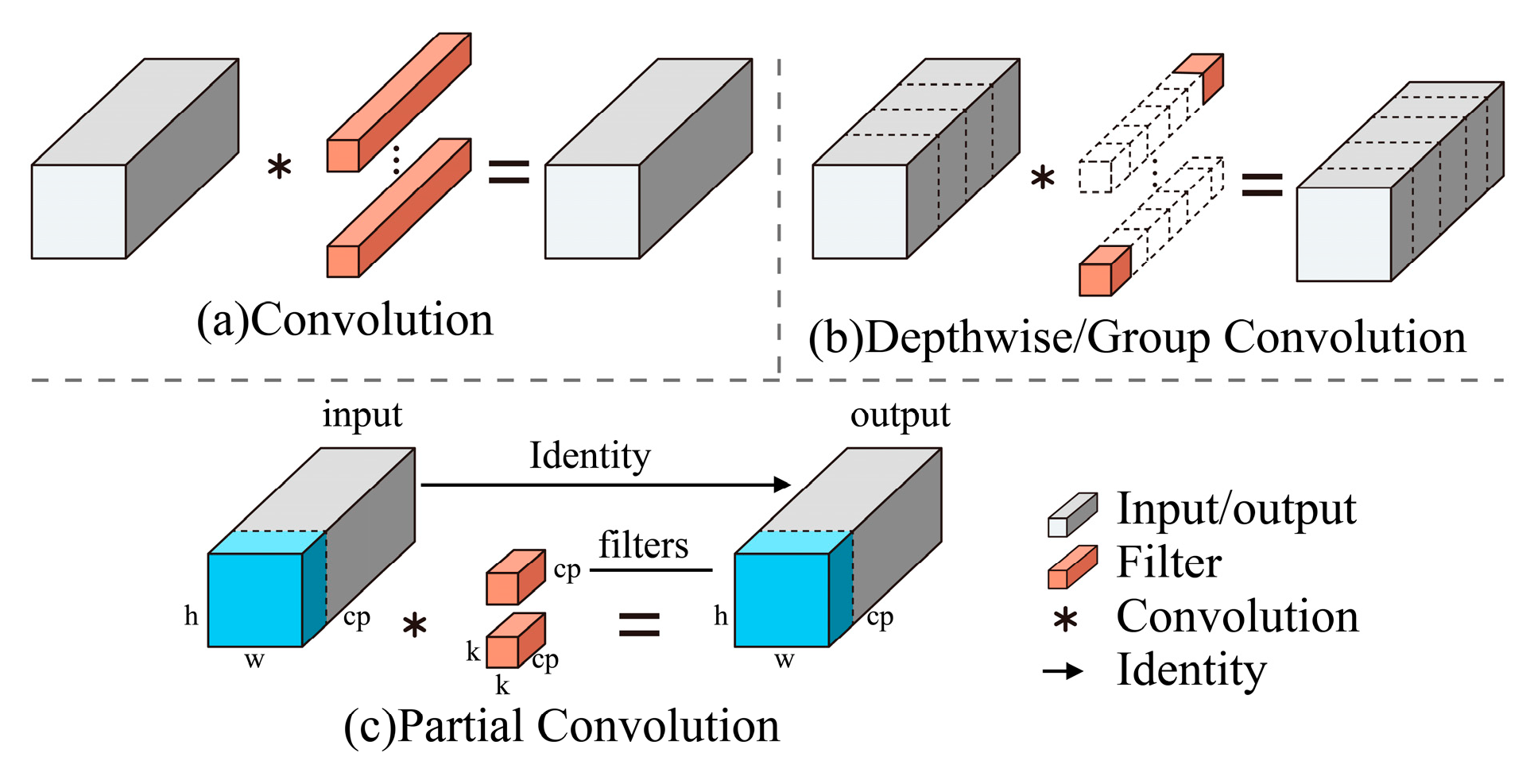
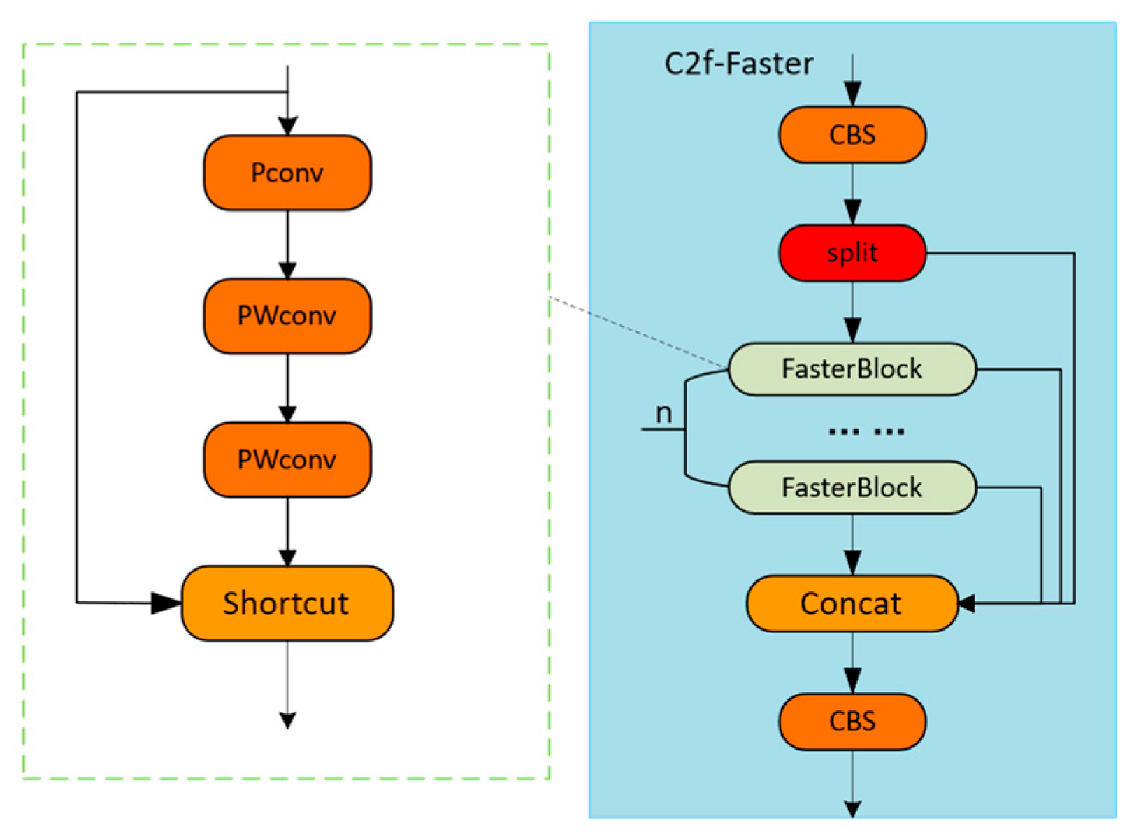
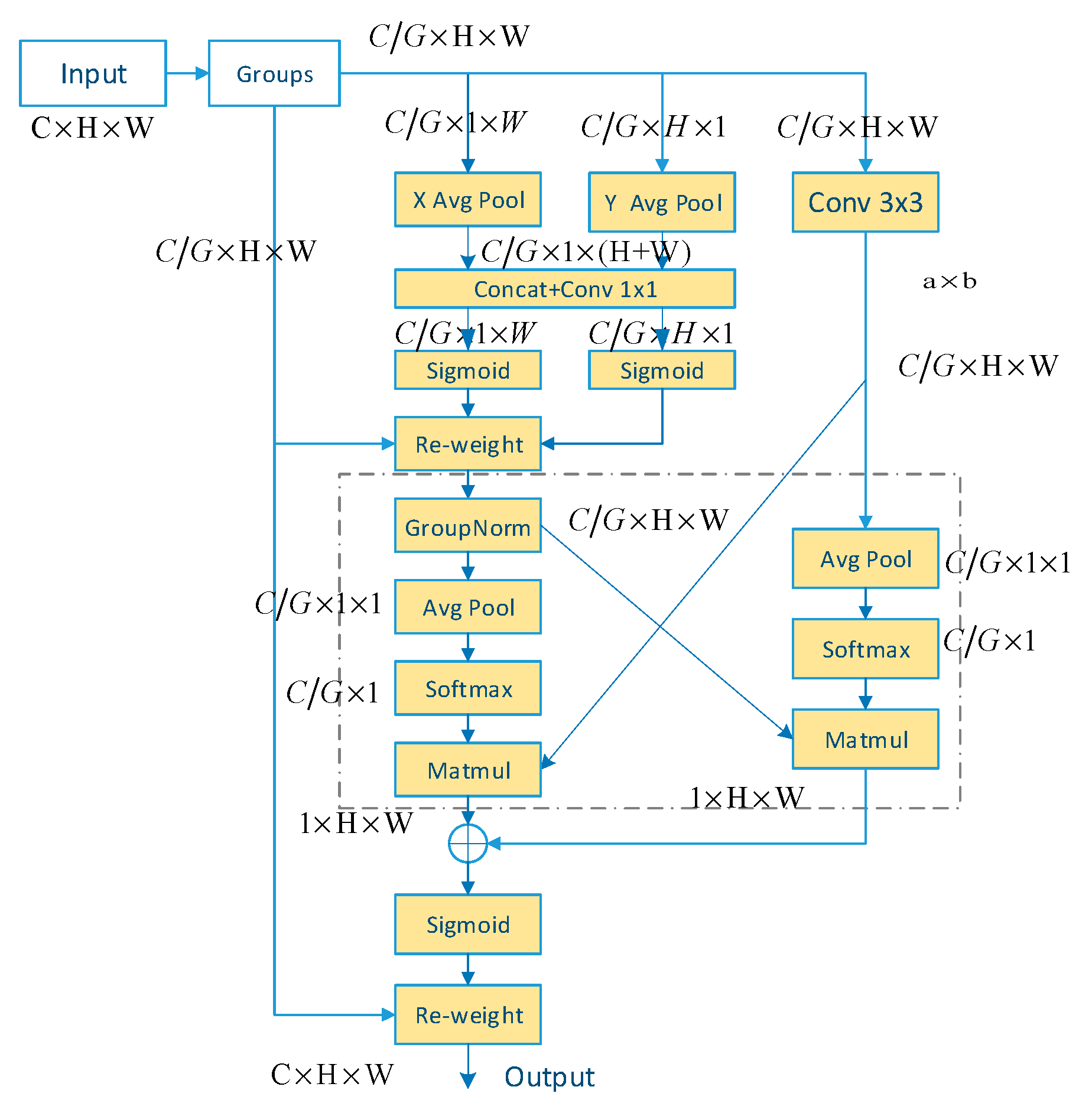
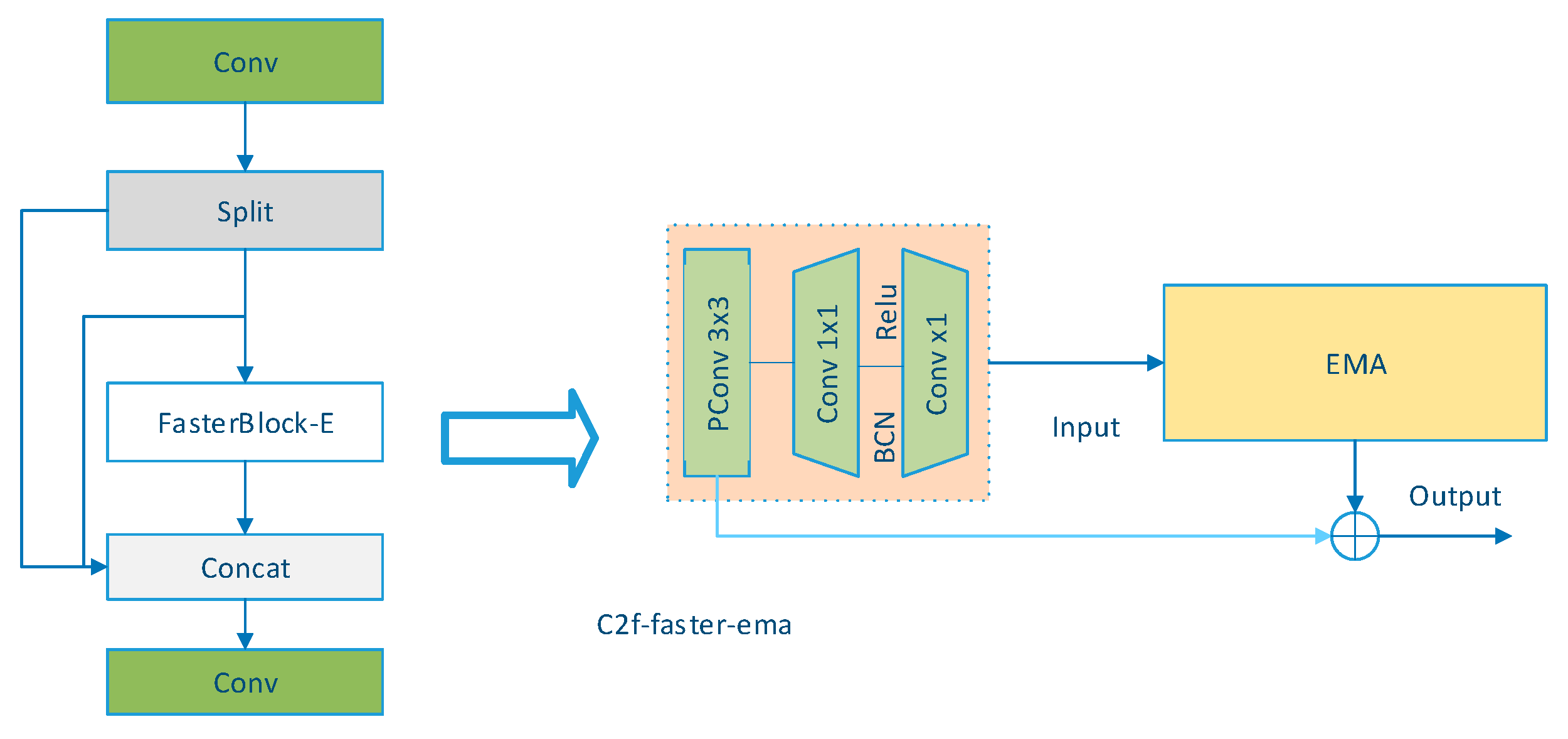
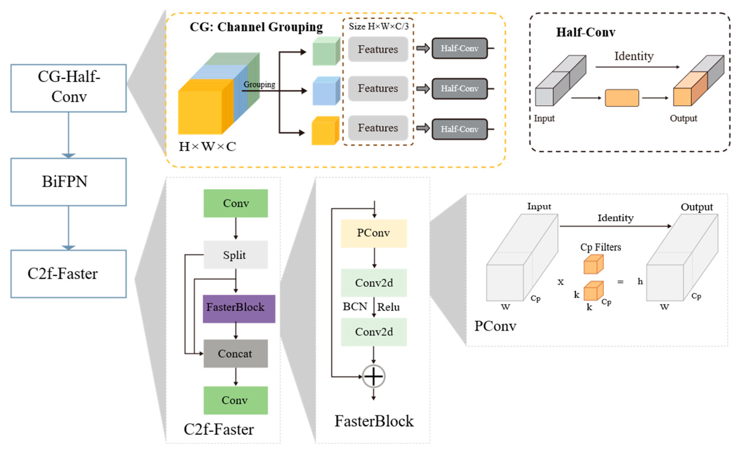
2.3.1. Architectural Optimization for Lightweight Detection

Due to the different target sizes and low image resolution in the scene of Torreya male cones in the natural environment, the flower information will gradually lose detailed information in the high-order feature map. The C2f (as Figure 4) module in YOLOv8s mainly uses conventional convolution for feature extraction, which not only causes the accumulation of redundant information and increases the computational burden on the network, but may also lead to false detections and missed detections. In order to solve the above problems, this study used FasterNet [19] to re-build the backbone feature extraction network of YOLOv8. FasterNet proposes a novel PConv, which can reduce computational redundancy and memory access at the same time and improve the detection speed of the model. It exploits redundancy in feature maps and systematically applies regular convolutions (Conv) on only a subset of input channels without affecting the remaining channels. For consecutive or regular memory accesses, PConv treats the first or last consecutive channel as a representative of the entire feature map for calculation, and considers the input and output feature maps to have the same number without loss of generality.
The FasterBlock module (Figure 5) achieves a significant reduction in the number of parameters and floating-point operations by fusing partial convolution (PConv) with pointwise convolution (PWConv). Specifically, PConv reduces both the number of parameters and computational complexity by performing convolution operations on only selected channels of the input feature map, whereas it still maintains efficient feature extraction capabilities [20,21]. Furthermore, by introducing sparse convolution mode and connection sparsity, PConv enhances the model's compression rate without compromising accuracy, thereby establishing a solid foundation for real-time reasoning on mobile devices. Building on this, PWConv employs pointwise convolution to facilitate feature fusion from the output of PConv. This operational mode not only preserves the spatial resolution of features but also enables cross-channel interaction at a lower computational cost, further enhancing computational efficiency.
Figure 6 illustrates PConv, an innovative convolution operation presented in FasterNet, which minimizes redundancy through its mechanism for partial channel processing while preserving the ability to represent features effectively. Unlike previous convolution methods that convolve all channels of the input feature, PConv only performs conventional convolution on a part of the channels of the input feature. Features are extracted and other channels are not processed. For the continuity of memory access, the first or last consecutive channels are usually selected to represent the entire feature map. Therefore, PConv greatly compresses the parameters and calculations, and still maintains good feature extraction capabilities. As in Equation (1), when cp is 1/2 of c, compared with conventional convolution, the FLOPs of PConv are only 1/4 of conventional convolution [21,22].
F C o n v = h × w × k 2 × c 2 F DConv = h × w × k 2 × c F PConv = h × w × k 2 × c p 2
where: h and w denote the height and width of the input image, respectively, k represents the kernel size, and c and c p both represent the number of input channels.
The C2F (Cross Stage Partial Fusion) module in YOLOv8 demonstrates effective feature reuse and multi-scale information integration capabilities through its cross-stage feature fusion mechanism in general object detection tasks. However, when applied to Torreya grandis male cone detection in natural environments, this module exhibits critical bottlenecks: computational redundancy & real-time deficiency.
To address these limitations, we propose the C2F-Faster module(Figure 7), which implements dual-phase architectural enhancements to achieve computational efficiency, yet maintaining detection precision.
The backbone network architecture proposed in this chapter is illustrated in Figure 8. The improved backbone first extracts spatial-channel information from the input image through a stack of convolutional layers, generating low-level feature maps. Subsequently, a C2f-Faster module performs efficient downsampling and feature compression. This module utilizes a dual-path architecture to achieve a coordinated reduction in spatial dimensions and an expansion in channel dimensions. For feature enhancement, a C2f-FE module is incorporated, which embeds an EMA attention mechanism. This mechanism performs cross-channel semantic modeling on the primary features, dynamically amplifying the feature responses of key regions such as mature Torreya grandis 'fruits' and enabling adaptive feature recalibration. Finally, in the multi-scale fusion stage, an SPPF module integrates multi-scale contextual information. It applies spatial pyramid pooling at scales of 5×5, 9×9, and 13×13, followed by concatenation and a depthwise convolution to fuse global and local context, thereby producing high-level semantic feature maps. These final features provide robust representational support for the subsequent object detection task. Collectively, these modifications result in a lightweight backbone design.

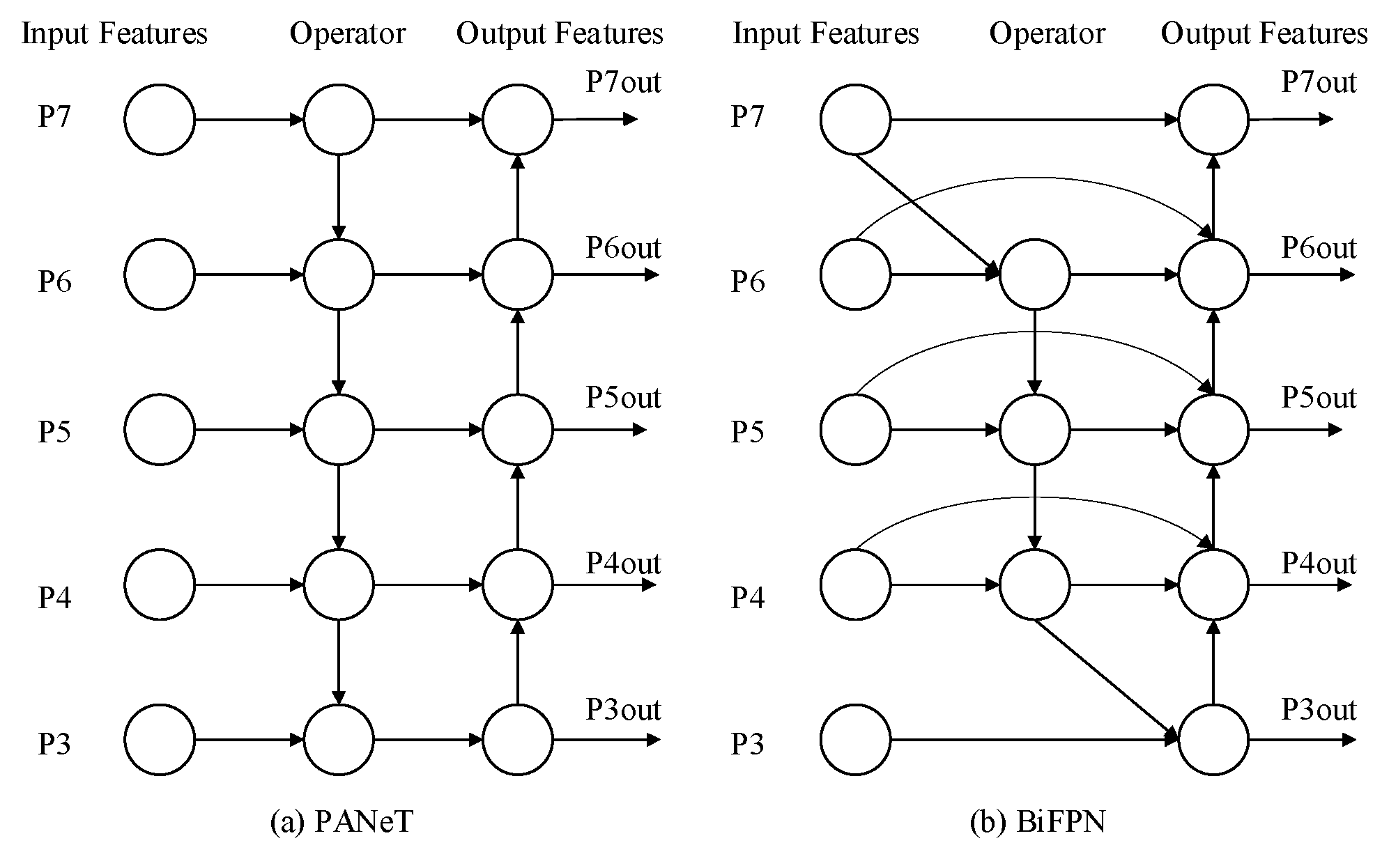
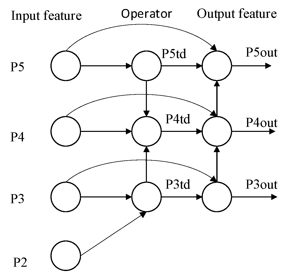
2.3.2. Enhancement of the Neck Network

(1) EMA convolution attention mechanism module
Integrating the attention mechanism into deep learning architectures enhances the model's capacity to concentrate on critical information within the input data, thereby optimizing its overall performance. The attention mechanism effectively emphasizes locally significant information, enabling the model to focus more on the relevant features of the detection object. Consequently, it has been widely adopted in various computer vision tasks across different fields.
EMA [23], it’s an efficient multi-scale attention mechanism. Its ability to reduce computational costs while preserving the information of each channel stems from its capability to reshape certain channels into batch dimensions, effectively preventing channel dimensionality reduction. Compared to other attention mechanisms, EMA offers two significant advantages: first, it enables the adjustment of parallel sub-network channel weights through global information encoding; second, the output features of its two parallel sub-networks are achieved through cross-latitude interaction.
Figure 9 illustrates the overall structure of EMA. For any input feature   X R C × H × W , in order to learn different types of semantics, EMA divides X into G sub-features in the cross-channel direction, and the input feature X = [ X 0 , X i , , X G 1 ] , X i R H × W , weight symbols to enhance. The input tensor shape is defined as, which includes 2 branched parallel branches and 1 branch path. By adopting a one-dimensional global average pooling operation in two horizontal/vertical dimensions in the branch, the dependencies between all channels can be obtained while reducing the amount of calculation [24]. The data feature processing operations are as follows:
In the EMA module, a multi-branch processing mechanism is employed. The input data is initially divided into multiple groups, which are then analyzed through distinct processing branches. Here, "g" denotes the number of groups into which the input channel is partitioned. "XAvgPool" and "YAvgPool" refer to one-dimensional horizontal and vertical global pooling operations, respectively [25]. On the one hand, one branch is responsible for performing a one-dimensional global pooling operation, while on the other hand, the other branch performs feature extraction through a 3×3 convolution kernel. The output features generated by the two branches are then subjected to nonlinear transformation through the sigmoid function to introduce more nonlinear factors and enhance the expression ability of the model. At the same time, Batch Normalization (BN) processing is applied to these features to speed up the training process and improve the generalization ability of the model. Next, these processed features are fused through the cross-dimensional interaction module. The core of this module is to effectively capture pixel-level pairwise relationships, that is, the correlation between pixels at different locations. Through cross-dimensional interactions, the module can integrate feature information from different branches to form a more comprehensive and accurate feature representation. Finally, after being processed by another sigmoid function, the output feature map is used to enhance or weaken the original input features. This step dynamically adjusts based on the importance of features to ensure that the model can focus on those features that are most critical to the current task.
(2) The Faster-EMA module proposed
As depicted in Figure 10 innovatively integrates the lightweight architecture of the FasterNet Block with the EMA attention mechanism. The original FasterNet Block employs a dual-path design: the main path comprises a 3×3 PConv, a CBS module, and a Drop Path of standard convolution, along with the skip connection from PConv. To enhance the feature representation capability, we embed the EMA module after the 1×1 convolution in the main path, thereby establishing a new feature enhancement path. The final output is generated by fusing the enhanced Drop Path with the skip connection features. This design preserves the efficiency of the FasterNet Block while achieving cross-channel semantic modeling through the EMA mechanism, enabling the module to capture richer contextual information without significantly increasing computational load, thereby balancing accuracy and efficiency.Weighted Bidirectional Characteristic Pyramid Structure. This design is particularly crucial for detecting Torreya male cones in real-world orchard settings, where cameras mounted at high positions for broad coverage necessitate robust multi-scale target detection capabilities.
(3) Lightweight BiFPN for Multi-scale Feature Fusion
The neck network of YOLOv8 continues the PANet [26] structure of YOLOv5. In the PANet architecture, the FPN module transfers high-level semantic features to the lower levels in a top-down manner. This supplements the semantic information in the low-level features, resulting in feature maps that are both semantically strong and high-resolution, which is beneficial for small object detection. Subsequently, the PAN module utilizes a bottom-up path to transfer low-level spatial details to the higher levels, ensuring this information is fully leveraged. Ultimately, this design achieves effective multi-scale feature fusion. However, this bidirectional feature fusion inevitably leads to an increase in parameters and computational cost. At the same time, the PANet structure also contains many nodes with only one input edge. These nodes have limited contribution to the feature fusion network, but increase the model’s efficiency. parameter quantity. Therefore, this paper introduces a more lightweight and efficient weighted bidirectional feature pyramid network (BiFPN).
As depicted in Figure 11, BiFPN optimizes the network architecture by strategically pruning fusion nodes with single-edge connections—unlike PANet's symmetrical bidirectional fusion structure. In addition, BiFPN also adds an additional connection between the original input and output nodes at the same level (with a consistent number of channels), and the network learns the weights of different input features, achieving more features without increasing the computational cost of information fusion [27].
To better adapt to the specific task of detecting small-sized Torreya male cones, the feature hierarchy is tailored. The original BiFPN, designed for general object detection, utilizes feature levels from P3 to P7. In this work, the higher-resolution P2 level is introduced as input, while P3 to P5 are retained as outputs. This modification is critical because the P2 level, with its finer spatial details, provides essential visual cues for identifying small and dense targets. Simultaneously, omitting the deeper P6 and P7 layers streamlines the network to focus on the most relevant feature scales for the objects of interest, achieving an optimal balance between accuracy and computational efficiency—a crucial consideration for a lightweight, real-time detection system.
BiFPN achieves weighted feature fusion through fast normalization, which is defined in Equation (2). Use the ReLU activation function to limit the weight w i to a non-negative value, and set ε to 0.001 to ensure numerical stability. At the same time, because the Softmax operation is avoided, the training speed is greatly improved. Because of the characteristics of bidirectional cross-scale connection and fast normalized feature fusion, BiFPN, a multi-feature fusion model, is more suitable for a lightweight real-time detection system of Torreya male cones.
O = i w i ε + j w j I i .
In Equation (2), O is the fused feature map, I i represents the i-th input feature map to be fused, w i and w j are automatically learned weights, and ε is a very small number to prevent numerical instability. The weights of the control parameters are distributed within the range of 0 to 1, and the ReLU activation function is employed to ensure the weight values remain non-negative. By normalizing the data, its maximum value is constrained to 1.
In the improved BiFPN architecture, this fusion method is applied to every cross-scale connection. Taking the fusion process that generates the final output feature P 4 in Figure 12 as an example, its specific computation is shown in Equation (3):
P 4 t d = C onv ( w 1 P 4 i n + w 2 Res i z e ( P 5 i n ) w 1 + w 2 + ε ) P 4 o u t = C onv ( w 1 P 4 i n + w 2 P 4 t d + w 3 Res i z e ( P 3 o u t ) w 1 + w 2 + w 3 + ε )
where: P 4 i n represents the feature map extracted from the 4th layer of the backbone network, whose resolution and semantic level vary with increasing i.  p 4 t d is the intermediate layer, obtained by weighted fusion of the 4th layer backbone feature ( P 4 i n ) and the upsampled 5th layer feature (Resize( P 5 i n )). p 3 o u t is the final output feature of the 3rd layer. w 1 , w 2 , w 3 are learnable weight parameters that are automatically optimized through backpropagation to balance the contributions of different features. ε is a stability constant to avoid division by zero errors.
This study introduces a Channel Grouping Half Convolution (CG-Half-Conv) [28] layer before the BiFPN. This operation performs lightweight grouping and half convolution processing on the input features prior to multi-scale fusion in BiFPN, aiming to enhance feature diversity and discriminability. By doing so, it improves the representation capability of subsequent feature pyramids for small targets like Torreya grandis male flowers without significantly increasing computational overhead.
F C G H a l f C o n v = h × w × k 2 × c b 2
M C G H a l f C o n v = h × w × 2 c b + k 2 × c b 2 h × w × 2 c b
Y = C o n c a t { C o n v X h , w , 0 : c / 2 , X h , w , 1 + c / 2 : c }
In Equation (4)-(6), we define the parameters as follows: h and w denote the height and width of the input image, respectively, k represents the kernel size, and c is the number of input channels. Where concat denotes the concatenation operation, conv represents the convolution operation, and X is the input feature map.
CG-Half-Conv serves as the core for achieving efficient feature enhancement. As demonstrated in Equations (4) and (5), it exhibits significant advantages in both computational load and memory access. The specific operation involves: dividing the input feature map X into three groups along the channel dimension, performing feature extraction on each group via half-convolution separately, and finally concatenating the three output groups along the channel dimension to obtain the output feature map Y . This "grouping-half-convolution-concatenation" mechanism, through multiple independent and parallel convolutional operations, can more sensitively capture diverse discriminative features in images while improving computational efficiency.
To further enhance the efficiency of multi-scale feature fusion, we design a lightweight pre-processing module placed before the BiFPN. This module, termed the Grouped & Squeeze Channel (GSC) module, employs a grouped convolution followed by a pointwise convolution to halve the channel dimensions. This design achieves two main purposes: 1) it significantly reduces the computational cost and parameters prior to the computationally heavy BiFPN; 2) it encourages cross-channel interaction within groups, refining the feature representation for subsequent fusion. The integrated GSC-BiFPN structure allows for more efficient and effective multi-scale feature integration in our model, As depicted in Figure 13.

2.3.3. Improve The Loss Function

The bounding box loss function of YOLOv8 uses CIoU, as in Equation (7)-(9). Compared with the traditional IoU calculation method, CIoU improves the convergence speed of the model by introducing the distance and size information between the predicted box and the real box in the penalty term.
CIoU = IoU ρ 2 ( b , b gt ) c 2 + α v
where: IoU represents the intersection over union (IoU) between the predicted bounding box produced by the model and the ground truth box, with values ranging from 0~1. The variable c denotes the diagonal length of the minimum circumscribed rectangle that encompasses both the predicted and the ground truth boxes. The term ρ 2 ( b , b g t ) indicates the distance between the center point of the predicted box and that of the ground truth box. Additionally, the parameters α and v are employed to evaluate the consistency in size between the model's predicted box and the actual box [29]. α is a weighing factor to balance the contribution of v , given by:
α = v ( 1 IoU ) + v
v = 4 π 2 arctan w gt h gt arctan w h 2
Here, w gt , h g t , w , h are the width and height of the ground truth and predicted bounding boxes, respectively.
Due to the relatively small proportion of Chinese Torreya male cones within the visual target area and the vast number of negative samples, the model spends considerable time processing these negative samples and penalizing them (i.e., adjusting weights to reduce their contribution to the loss function) during the training process. When the model is trained using the CIoU loss function, this imbalance between positive and negative samples exacerbates the penalty on negative samples, thereby prolonging the training time and potentially compromising the accuracy and generalization ability of the model's training results. Therefore, this algorithm adopts the Wise-IoU [30] (WIoU) as the loss function, dynamically assessing anchor box quality based on outlier degrees to mitigate the interference of negative samples on model quality, that is:
L WIoU = r R WIoU L IoU
r = β δ α β α
L I o U = 1 I o U
where: β represents the outlier degree, which is negatively related to the quality of the anchor box; α and δ represent the hyperparameters with values 1.9 and 3 respectively; RWIoU is the penalty term of WIoU. Setting WIoU as the bounding box loss function can effectively improve the influence of ordinary anchor boxes and avoid poor detection results of male cones due to small size, blur, occlusion and other problems.
R WIou = exp x x gt 2 + y y gt 2 W g 2 + H g 2
where: x ,y and x g t , y g t are the center coordinates of the predicted and ground truth bounding boxes, respectively, W g , H g represents the width and height of the smallest enclosing box which covers b , b g t .

2.4. Pruning-Based Lightweighting Improvement

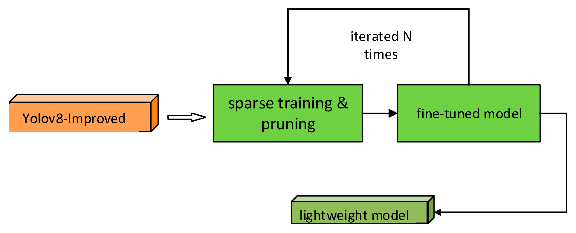
2.4.1. Model Pruning

As one of the main methods of model lightweighting, model pruning cuts out unimportant connections in the network structure, compressing the model size while maintaining model accuracy at a level comparable to the original model. The development of model pruning can be traced back to the proposal of the optimal brain loss algorithm in 1990. Since then, with the rapid development of deep learning, more and more experts and scholars have made outstanding contributions in the field of model pruning. In recent years, scholars such as Evci et al. [31] have discovered that when the layered sparsity is properly selected, the ideal pruning effect can be achieved by simply using the weight amplitude as the basis for pruning. However, existing pruning algorithms achieve hierarchical sparsity settings through manual experiments or hyperparameter searches. Manual experiments require a lot of manpower and material resources, and hyperparameter searches place high demands on equipment computing power.

2.4.2. YOLOv8s-Improved Pruning Algorithm Design

This article explores pruning methods and compares three different approaches. Through analysis in Chapter 4.6, the most suitable pruning method for the YOLOv8s-improved network based on the flowering stage maturity detection of Torreya male bulbs was obtained.
1) LAMP pruning method
LAMP is an amplitude-based layer adaptive sparsity pruning method proposed by Jaeho Lee [32] and others in 2021. The core idea of this method is to dynamically adjust the pruning ratio of each layer of the neural network model according to needs. Unlike pruning the entire network at once, the LAMP algorithm adopts layer-by-layer pruning. This layer-by-layer pruning method helps maintain the overall structure of the network and reduces the impact on model performance.
2) BNScaleImportance pruning method
The core idea of the BNScaleImportance [33] method is to utilize the scale parameter (γ) within the Batch Normalization (BN) layer to indicate the importance of each channel or neuron. In the BN layer, the γ parameter serves to linearly transform the normalized data, thereby restoring its expressive capability. Consequently, the magnitude of the γ parameter reflects the contribution of the respective channel or neuron to the model output. Specifically, channels or neurons with larger γ values exert a greater influence on the model output, whereas those with smaller γ values have a diminished impact.
3) MagnitudeImportance pruning method
MagnitudeImportance [34], it is a key evaluation method in neural network pruning and model compression. It aims to accurately evaluate the importance of neurons or channels by quantifying their contribution to model output. This method is based on the consideration of weight amplitude, believing that neurons or channels with larger weights carry more critical information and have a significant impact on model performance.

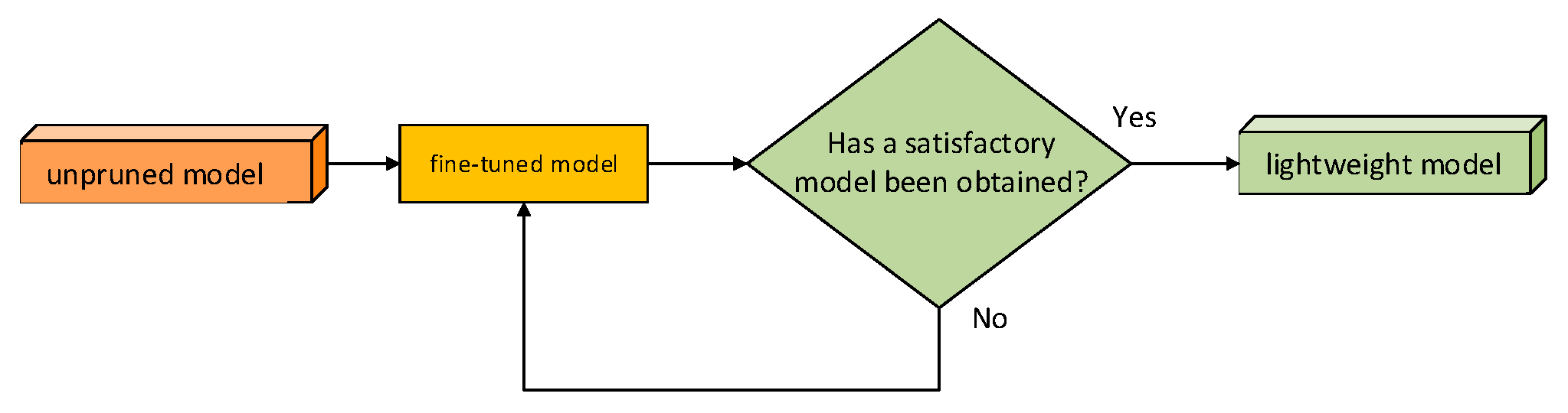
2.4.3. Pruning Model Fine-Tuning

Due to the continuous adjustments in the network structure during sparse training and pruning, the network cannot achieve its highest accuracy. To attain the optimal accuracy of the model, fine-tuning is essential. As illustrated in Figure 14 this study employs 'best.pt' as the pre-training weight during pruning and backtracking, utilizing a low learning rate for fine-tuning. Multiple iterations are conducted until satisfactory results are achieved. In each iteration, the model is evaluated, and the fine-tuning strategy is adjusted based on the outcomes.
The model trained by the neural network contains some relatively small weights. Although these parameters play a small role in the reasoning process and have little impact on the detection accuracy, they occupy numerous parameters. Therefore, this article will integrate YOLOv8s-improved and pruning algorithms to lightweight the model and reduce parameters and calculations as much as possible while ensuring accuracy. In the pruning process, this article adopts a structured pruning method. First, sparse training and pruning are performed simultaneously, and then the pruned model is fine-tuned and trained to obtain the final model.
Figure 15 illustrates the concurrent execution of sparse training and network pruning within our end-to-end optimization pipeline. First, this paper starts with an initial dense model and introduces sparsity through sparse training. Sparsity makes it easier to select parameters with smaller weights, thus facilitating pruning operations. Then, when sparsely training the model, we prune it structurally, removing entire neurons or layers. After pruning, this paper performs fine-tuning training on the pruned model to restore the performance of the model and further improve the accuracy. In the end, this paper obtained a final model with smaller parameters and stable detection performance within a certain accuracy range. It can be deployed in scenarios such as mobile devices to achieve accurate and real-time detection of the maturity of Torreya male cones.
Pruning during training is also called pruning with rewinding. In this method, the training and pruning of the model are performed alternately. The model will be pruned periodically during the training process, and the changes during the training process will be retained. The best model is used as the final model. In this pruning process, this chapter lightens the YOLOv8n-improve model by setting different pruning rates and different pruning methods, and finally obtains compression models with different parameter amounts.
In summary, Figure 16 illustrates the architecture of our proposed YOLOv8-c2f-Faster-EMA detection model. Building upon YOLOv8s baseline, we implement key enhancements including: (1) backbone feature extraction network upgraded with C2f-faster and C2f-faster-EMA modules combined with SPPF for multi-scale feature fusion, (2) neck network optimized through BiFPN modules and upsampling layers for enhanced feature pyramid fusion and small target detection, (3) head network refined via BiFPN integration and depthwise separable convolution layers to balance precision and efficiency, and (4) systematic model compression using network pruning techniques to reduce computational burden while preserving detection capability. These structural innovations collectively enable efficient feature extraction, robust multi-scale detection, and lightweight deployment for natural environment applications.

2.5. Evaluation Metrics

Metrics used when evaluating model performance include precision (P), recall (R), mean average precision (mAP), model weight size, number of parameters, FLOPs, and inference speed. The precision rate represents the proportion of correct predictions, the recall rate represents the proportion of correctly predicted categories to the total number, and mAP can comprehensively evaluate the accuracy and robustness of the algorithm. Inference time and network parameter volume are also used as performance metrics. Shorter inference times and smaller model sizes mean better real-time performance and memory utilization efficiency. In this study, indicators such as true positives (TP), false positives (FP), and number of missed true positives (FN) were used to evaluate the detection of Torreya male cones. The average accuracy value represents the average prediction accuracy for each category. The calculation formula is as in (14)-(17): The relevant calculation formula is as follows:
P = T P T P + F P × 100 %
R = T P T P + F N × 100 %
A P i = 0 1 p ( r ) d r
mAP = i = 1 C A P i C × 100 %
where: TP is the number of correctly predicted targets as positive samples, FP is the number of incorrectly predicted non-targets as positive samples, FN is the number of missed actual targets, C is the number of categories, and A P i is the average precision of the i-th category. Accuracy value, mAP is the average accuracy value of all categories.

3. Results and Analysis

3.1. Experimental and Parameter Settings

The algorithm model in this study was tested on the Ubuntu 22.04 operating system, with a detailed configuration of the experimental environment provided in Table 2. The dataset utilized was a self-constructed dataset, comprising a total of 2,648 images, which were partitioned into training, validation, and test sets in an 8:1:1 ratio. To improve the model's adaptability and enhance sample diversity during data processing, a built-in data augmentation module was employed, specifically adjusting the hue value by 0.013 within the HSV color space.
The configuration of experimental parameters is adjusted based on model performance metrics and loss trends, where the analysis results of mean average precision (mAP@50) and loss function curves guide the optimization process of hyperparameters. Table 3 presents the final combination of training parameters determined after multiple rounds of tuning. During the parameter optimization process, a dynamic adjustment strategy is employed to ensure the effectiveness of model training, and precise control over parameter settings is achieved through continuous monitoring of key performance indicators.

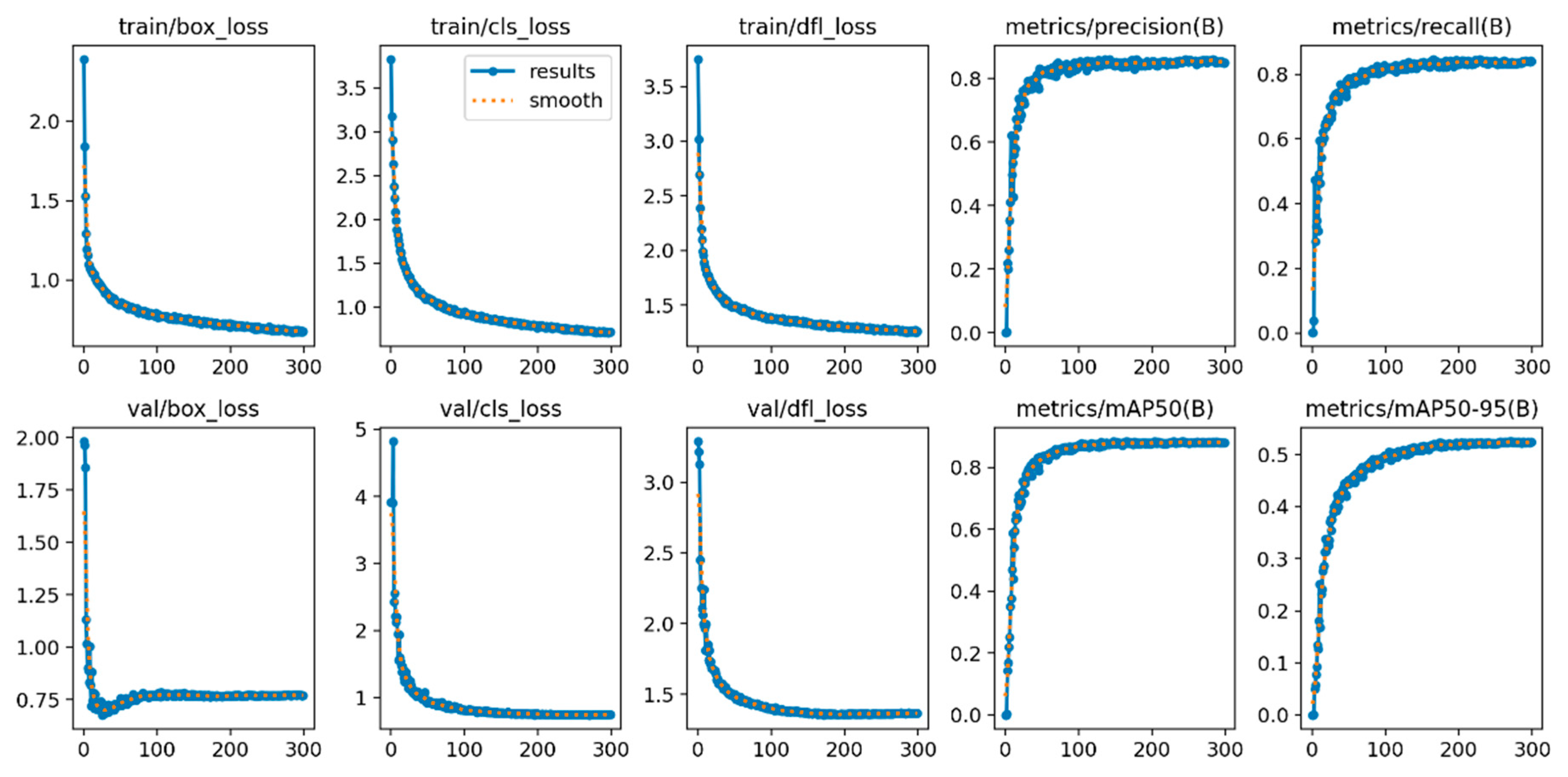
3.2. Analysis of Training Dynamics

As illustrated in Figure 17, from the training loss curves, it can be observed that the bounding box loss, classification loss, and distribution focal loss all decrease rapidly during the initial stages of training. Specifically, the box loss on the training set drops from an initial value of approximately 2.25 to around 0.5, the cls loss decreases from 3.75 to about 0.75, and the dfl loss declines from 3.65 to roughly 0.6. This significant reduction in losses indicates that the model is progressively learning effective feature representations and optimizing its predictive capabilities. A similar trend is also observed on the validation set. The box loss, cls loss, and dfl loss on the validation set gradually decreased during the training process, stabilizing at approximately 0.75, 0.75, and 0.5 respectively. The close alignment between validation loss and training loss indicates that the model did not suffer from severe overfitting and demonstrates good generalization capability.
The low and convergent loss values indicate that the model effectively optimizes its predictions for target localization and classification. This stable and efficient learning process underpins the model's enhanced capability in accurately detecting the maturity stages of Torreya male cones.

3.3. Ablation Experiments

To validate the contributions of the C2F lightweight design, BiFPNCH feature fusion enhancement structure, and attention mechanism in the proposed method, this study systematically evaluates the model optimization effects through eight sets of controlled experiments, with ablation study results presented in Table 4. The ablation experiments systematically investigate the independent and collaborative optimization effects of the C2f-f lightweight module, EMA, and BiFPNCH on the YOLOv8 object detection model. The experimental design adopts a progressive module integration strategy. The baseline model achieves 85.1% precision, 81.5% recall, and 86.3% mAP@.50, with model weights and computational costs of 22.5MB and 28.8G FLOPs respectively. The standalone introduction of the C2f-f module significantly enhances mAP50 to 88.3% while markedly reducing model complexity, with weights and FLOPs decreasing by 24.9% and 25.7% respectively, demonstrating its lightweight advantages through structural reparameterization. EMA improves recall by 3.2 percentage points to 84.7% via cross-dimensional feature enhancement, validating the feature discrimination capability of the Torreya grandis male flower recognition model in complex scenarios. BiFPNCH enhances model performance with mAP@.50 reaching 88.3% while substantially reducing model weights (from 22.5 to 15.1). Module combination experiments further reveal technical synergies. First, the combination of C2f-f and EMA maintains lightweight characteristics while achieving the highest mAP@.50 (88.9%). Second, the integration of C2f-f and BiFPNCH achieves a 39.2% reduction in computational load. Finally, the three-module fusion demonstrates outstanding comprehensive performance. While maintaining optimal detection accuracy (mAP50 88.9%, recall 84.9%, F1-score 85.20%), the model weight and computational load are significantly reduced by 54.1% and 39.2% respectively. This proves the functional complementarity of each module in feature extraction, attention enhancement, and multi-scale fusion, providing a lightweight solution for high-performance object detection in computationally constrained environments.
In summary, the combination of C2f-f, BiFPNCH, and EMA constitutes the optimal solution in terms of accuracy and lightweight design. Among them, C2f-f effectively reduces the model's parameter count and computational complexity while contributing to improved recall rates; BiFPNCH makes the most significant contribution to model lightweighting while maintaining detection accuracy through enhanced feature fusion; the EMA attention mechanism serves as the key component for boosting performance metrics such as recall rate.

3.4. Comparison of Attention Mechanisms

This study replaces the EMA attention mechanism in the C2f-faster module of the backbone network based on ablation experiment 4, and uses four different attention mechanisms to explore its impact on the model. The Table 5 show that among these replacements, the C2f-faster enhancement module using the EMA attention mechanism exhibits the best overall performance.

3.5. Comparison of Loss Functions

Regarding the selection of loss function, this paper proposes a new loss function that combines WIoU loss with NWD [40] loss to address the shortcomings of CIoU. In order to verify its effectiveness, the performance difference was compared with various mainstream regression losses, and experiments were conducted on a lightweight model after adding EMA attention. Table 6 quantifies the superior performance of our proposed regression loss algorithm, which achieves optimal recall-precision balance while attaining the highest mAP50 and mAP50-95 values among comparative methods. It is proved that the regression loss algorithm proposed in this article is the most suitable for smart agriculture task scenarios. It not only maintains the high-speed characteristics of WIoU loss, but also effectively improves the flowering maturity recognition accuracy of the model.

3.6. Sparse Training Experimental Comparative Analysis

A systematic analysis was conducted on the experimental data of the GFM-YOLO baseline network during the sparse training phase. As a critical preprocessing step for model compression, sparse training introduces an L1 regularization term (controlled by hyperparameter λ) to induce sparsity in network weights, laying the foundation for subsequent pruning operations. We configured the experiment with four distinct λ values (0.0005, 0.001, 0.005, and 0.01) to evaluate their impact on object detection metrics (precision P, recall R, and mAP@0.50), and recorded the corresponding parameter count and computational complexity of the model, as detailed in Table 7.
Table 7 shows that the model maintains high detection performance across different λ values. Specifically, the mAP@.50 exhibits minor fluctuations (88.3%~88.5%), indicating the inherent robustness of the GFM-YOLO network architecture. The model achieves optimal overall performance when λ=0.01, with mAP@.50 of 88.5%, R of 84.4%, and precision of 84.9%. Compared to other λ settings, this configuration maintains the highest mAP while achieving the best recall rate, which is crucial for ensuring comprehensive detection of Torreya grandis flowering targets. Furthermore, no significant performance degradation occurs with increasing λ values, demonstrating the model's tolerance to strong regularization constraints.

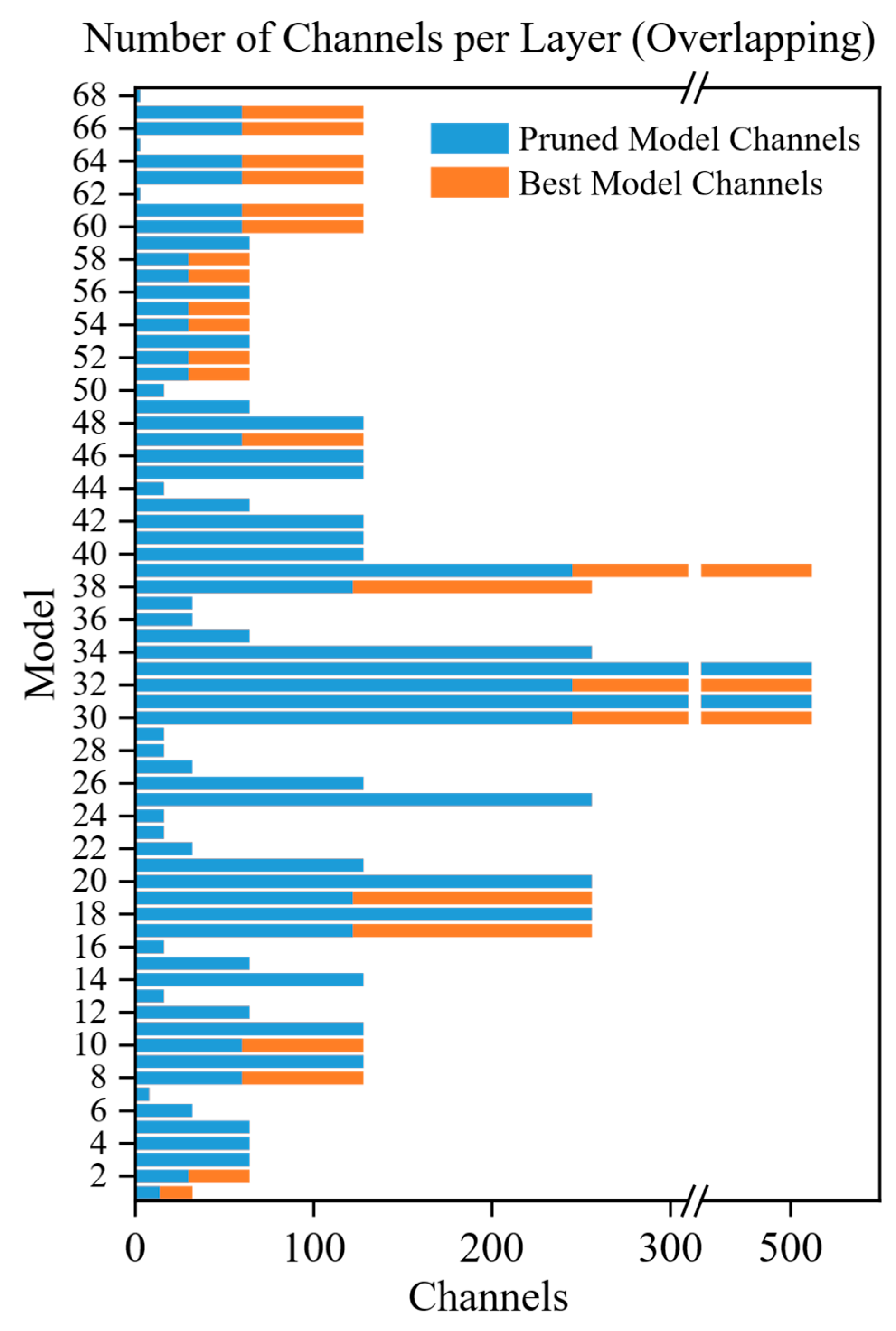
3.7. Model Pruning Experiment

In order to reduce the demand for computing power of intelligent edge devices as much as possible, this paper performs amplitude-based layer adaptive sparse pruning on the improved model. In order to explore the model performance under different pruning rates and select the most suitable pruning model for practical applications, this paper makes statistics on the model pruning effects under different pruning rates. Figure 18 demonstrates that low pruning rates improve model accuracy, indicating that the pruning method used in this article can remove redundant weight connections in the model and play a regularization role. When the pruning rate is greater than 0.5, the model accuracy begins to gradually decrease. When the pruning rate is greater than 0.7, the model size is greatly reduced, the representation ability is also affected, and the accuracy decreases rapidly. Taking into account the model's size and accuracy, this study selects a pruning rate of 51% and employs the refined model after pruning as the final structural design.
In order to verify the impact of LAMP, BNScaleImportance, and MagnitudeImportance pruning methods on model performance under different pruning rates, this paper conducted comparative experiments. Experimental results show that as the pruning rate gradually decreases, these three pruning methods all show a consistent trend: the model parameters are significantly reduced, the model volume is reduced accordingly, and the FPS (frame rate) is also improved to varying degrees. However, this process is also accompanied by a slight decrease in detection accuracy. After comprehensively referring to the data in Figure 18, Figure 19 and Figure 20, we found that in BN pruning mode, when the pruning rate is set to 0.51. At that time, the number of model parameters was successfully reduced by 58.4%, while mAP50 was still as high as 88.2%, and the accuracy loss was controlled within 1 percentage point; mAP50-95 was 52.0, and the loss was only about 0.5 percentage points. What is even more gratifying is that the FPS at this time reached 120.1 frames/second, which was a significant improvement of 76.3% compared to 68.1 frames/second before pruning.
Therefore, it can be considered that when the pruning rate is 0.51, the BN pruning method reaches the best balance between model performance and pruning effect.
As illustrated in Figure 20, this chart compares the frames per second (FPS) across three pruning methods: Lamp, BNperformance, and MagnitudeImportance, at varying pruning rates. Notably, as the pruning rate increases, there is a significant rise in FPS, primarily due to the reduction in the number of model parameters and overall model size. The comparison presented in Figure 20 indicates that when employing the BNperformance pruning method, the improvement in FPS is markedly superior compared to the Lamp and MagnitudeImportance methods at the same pruning rate.
To sum up, it can be concluded that the accuracy maintenance and model compression effect of the YOLOv8n-improved model using the BN pruning method is better than the other two pruning methods. Specifically, the BN pruning method can not only reduce the number of model parameters and model size more effectively, but also maintain better model accuracy under higher pruning rates. This makes the BN pruning method more advantageous in hot-rolled steel strip surface defect detection scenarios that require both model performance and resource optimization.

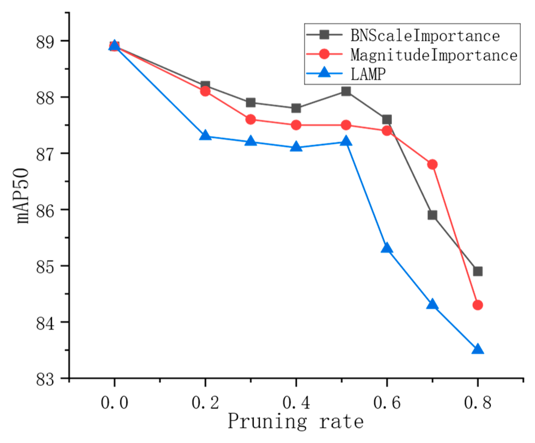
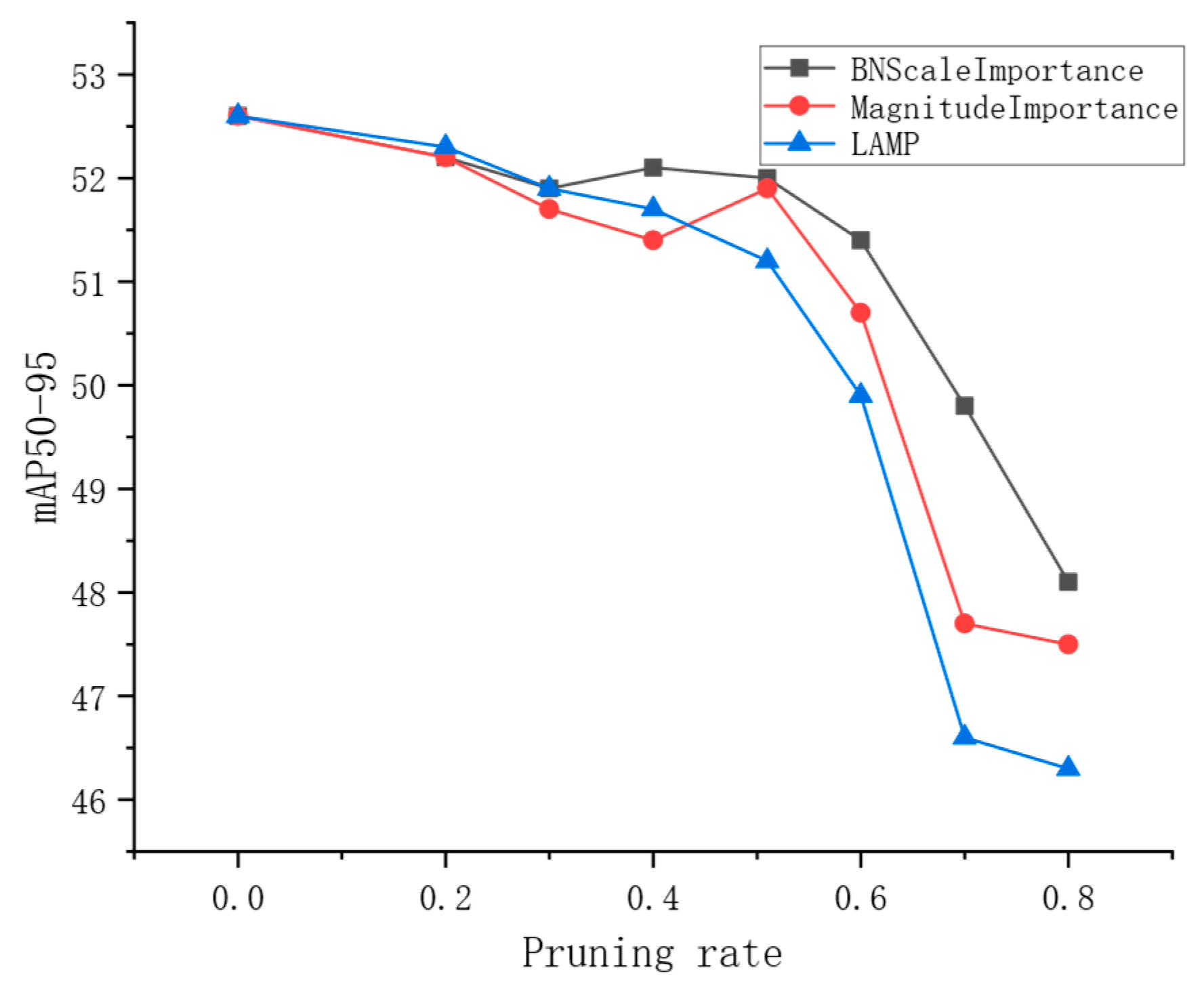
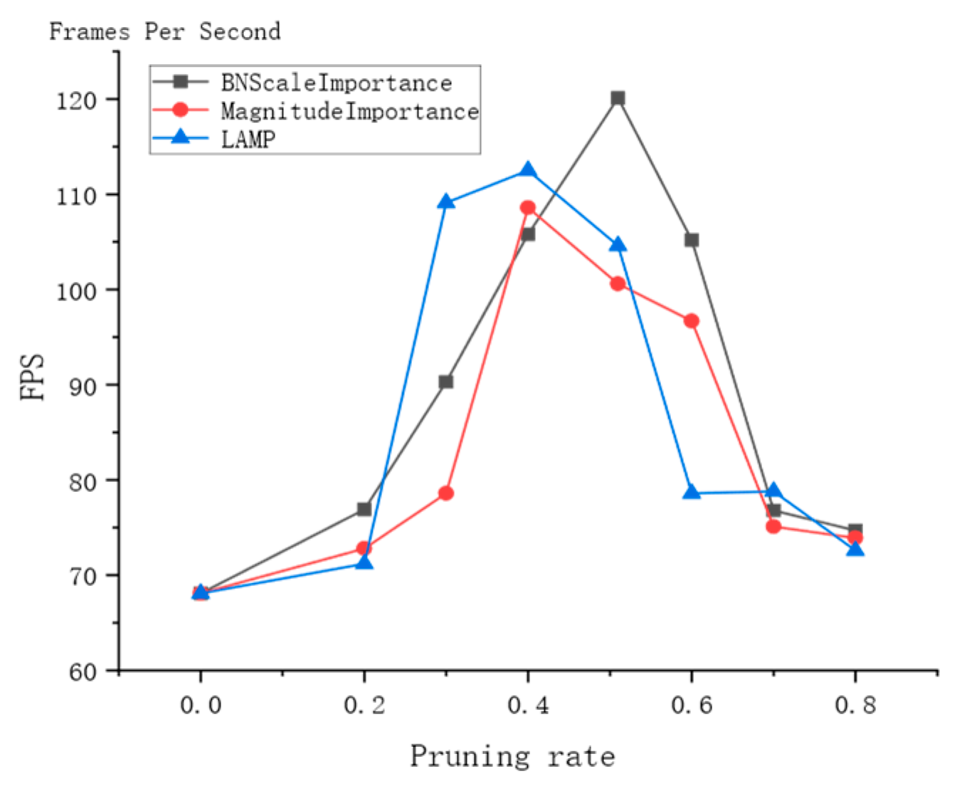
3.8. Analysis of Pruning Effects

Through pruning experiments and data analysis, it has been determined that the detection performance and pruning effect of the model achieve an optimal balance when the Bn pruning method is used and the pruning rate is set to 0.51. Figure 21 demonstrates the changes in the number of channels before and after pruning using this method. Specifically, "best" represents the model channels without pruning, whereas "prune" represents the model channels after pruning. It is evident that some less important channels are almost completely removed, whereas the number of channels in the improved model proposed in this paper remains largely unaffected. This phenomenon indirectly validates the effectiveness of the improvements made to the model. Therefore, by adopting a reasonable pruning strategy, it is possible to reduce model parameters and increase FPS, yet maintaining the detection accuracy of the model.

3.9. Comparison of Different Advanced Detection Algorithms

The improved model was compared with YOLOv4, YOLOv5s, YOLOv7-tiny, YOLOv8s,Yolov10s, RT-DETR-l, and the results are summarized in Table 8. We observed that the improved model reached 88.2% in terms of mean average precision (mAP50), which is significantly higher than other comparison models. In addition, this model is also significantly lower than other models in terms of performance indicators such as FLOPs, number of parameters, and weight size. It is worth noting that the detection time of GFM-YOLOV8 on GPU and CPU is 6.5 milliseconds and 55.3 milliseconds respectively, which makes it the shortest detection time among all compared models, and is 1.6 faster than the detection time of YOLOv8s. milliseconds and 5 milliseconds. Compared with models with the same level of accuracy, the compression rate of this model exceeds 56%. It proves the effectiveness and superiority of the improvement strategy proposed in this paper.
This study evaluated the GFM-YOLOV8 model for detecting flowering stage maturity in Torreya male bulbs under complex natural conditions. A test dataset was constructed from images with typical interference factors (e.g., occlusion, overlap, backlight, low light), and systematic detection experiments were performed.
Figure 22 presents a rigorous assessment of detection robustness under six diverse natural conditions, demonstrating the model's environmental adaptability. Through in-depth observation and scientific analysis of the results, we observed that even in the case where the growth environment of Torreya male cones is extremely complex and there are many interference factors, the GFM-YOLOV8 model still shows excellent recognition ability, able to accurately distinguish and identify Torreya male cones at different stages of maturity.

4. Conclusions

This study discusses the problem of rapid detection of the flowering stage maturity of Torreya male cones in the natural environment, and proposes the GFM-YOLOV8s Torreya male cone maturity detection model based on YOLOV8, and proves this method through comparative experiments. Study the superiority and robustness of the proposed improvement strategy.
1) In order to solve the problem of difficulty in detecting natural scenes of Torreya male bulbs and high real-time requirements, the backbone network was replaced with the c2f-faster network and the EMA was introduced into its head structure. The PAN-FPN feature extraction structure at the neck was replaced with the BiFPN structure, by removing nodes with small contributions and adding cross-layer connections, better integration and utilization of features at different scales are achieved, effectively improving the model’s feature extraction and integration capabilities in complex and changeable weather Torreya male cone flower scenarios. While reducing the amount of calculation and improving the detection accuracy and detection speed of target detection.
2) The WIoU loss function was used to solve the problem of loss function failure of the YOLOv8 target detection algorithm when targeting small-sized and long bounding box Torreya cones, which not only solved the problem but also improved the detection accuracy of the lightweight model.
3) Experimental results show that through training with the self-built data set of the Torreya Industry Alliance of Zhejiang A&F University, the mAP of the GFM-YOLOV8 model reached 88.9%. The GFLOPs is 8.7, the parameters is 2.2×10⁶, and its weight size is 4.4MB. Compared with the YOLOv8s model, GFM-YOLOV8 has significantly improved overall performance, specifically showing that mAP has increased by 2 percentage points. In addition, the GFLOPs, parameters, weight size and detection time were reduced by 69%, 80.1%, 79.2% and 19.7% respectively. Experiments show that GFM-YOLOv8s shows advantages in both efficiency and accuracy.
The conclusion shows that the improved GFM-YOLOv8s is superior to YOLOv8s in terms of technical implementation and performance. In particular, significant progress has been made in terms of parameters, GFLOPs, weight size, etc., which will provide better conditions for the growth of Torreya male cones. The monitoring visual identification system provides strong support.

Funding

The work was supported by the Central Fiscal Forestry Science and Technology Extension Demonstration Project ( grant no. TS04-2 ).

Institutional Review Board Statement

Not applicable.

Informed Consent Statement

Not applicable.

Data Availability Statement

The data presented in this study are available on request from the corresponding author. The data are not publicly available due to privacy.

Conflicts of Interest

The authors declare no conflict of interest.

References

  1. Wang, H.; Li, Y.; Wang, R.; Ji, H.; Lu, C.; Su, X. Chinese Torreya Grandis Cv.Merrillii Seed Oil Affects Obesity through Accumulation of Sciadonic Acid and Altering the Composition of Gut Microbiota. Food Science and Human Wellness 2022, 11, 58–67.
  2. Chen, X.; Niu, J. Evaluating the Adaptation of Chinese Torreya Plantations to Climate Change. Atmosphere 2020, 11. [CrossRef]
  3. Chen; Jin Review of Cultivation and Development of Chinese Torreya in China. Forests, Trees and Livelihoods 2019, 28, 68–78.
  4. Hu, S.; Wang, C.; Zhang, R.; Gao, Y.; Li, K.; Shen, J. Optimizing Pollen Germination and Subcellular Dynamics in Pollen Tube of Torreya Grandis. Plant science : an international journal of experimental plant biology 2024, 348, 112227. [CrossRef]
  5. Chen, W.; Jiang, B.; Zeng, H.; Liu, Z.; Chen, W.; Zheng, S.; Wu, J.; Lou, H. Molecular Regulatory Mechanisms of Staminate Strobilus Development and Dehiscence in Torreya Grandis. Plant physiology 2024. [CrossRef]
  6. Liu, L.; Li, Z.; Lan, Y.; Shi, Y.; Cui, Y. Design of a Tomato Classifier Based on Machine Vision. PLoS ONE 2019, 14, e0219803–e0219803.
  7. Guo, Q.; Chen, Y.; Tang, Y.; Zhuang, J.; He, Y.; Hou, C.; Chu, X.; Zhong, Z.; Luo, S. Lychee Fruit Detection Based on Monocular Machine Vision in Orchard Environment. Sensors 2019, 19, 4091–4091. [CrossRef]
  8. Xiao, B.; Nguyen, M.; Yan, W.Q. Fruit Ripeness Identification Using YOLOv8 Model. Multimed Tools Appl 2023, 83, 28039–28056. [CrossRef]
  9. Cometa, L.M.A.; Garcia, R.K.T.; Latina, M.A.E. Real-Time Visual Identification System to Assess Maturity, Size, and Defects in Dragon Fruits. Engineering Proceedings 2025, 92. [CrossRef]
  10. Zhu, X.; Chen, F.; Zheng, Y.; Chen, C.; Peng, X. Detection of Camellia Oleifera Fruit Maturity in Orchards Based on Modified Lightweight YOLO. Computers and Electronics in Agriculture 2024, 226, 109471–109471.
  11. Trinh, T.H.; Nguyen, H.H.C. Implementation of YOLOv5 for Real-Time Maturity Detection and Identification of Pineapples. TS 2023, 40, 1445–1455. [CrossRef]
  12. Chen, Y.; Xu, H.; Chang, P.; Huang, Y.; Zhong, F.; Jia, Q.; Chen, L.; Zhong, H.; Liu, S. CES-YOLOv8: Strawberry Maturity Detection Based on the Improved YOLOv8. Agronomy 2024, 14, 1353–1353. [CrossRef]
  13. Sun, H.; Ren, R.; Zhang, S.; Tan, C.; Jing, J. Maturity Detection of ‘Huping’ Jujube Fruits in Natural Environment Using YOLO-FHLD. Smart Agricultural Technology 2024, 9, 100670–100670. [CrossRef]
  14. Chen, W.; Jiang, B.; Zeng, H.; Liu, Z.; Chen, W.; Zheng, S.; Wu, J.; Lou, H. Molecular Regulatory Mechanisms of Staminate Strobilus Development and Dehiscence in Torreya Grandis. Plant Physiology 2024, 195, 534–551. [CrossRef]
  15. Redmon, J.; Divvala, S.K.; Girshick, R.B.; Farhadi, A. You Only Look Once: Unified, Real-Time Object Detection. CoRR 2015, abs/1506.02640.
  16. Zaremba, W.; Sutskever, I.; Vinyals, O. Recurrent Neural Network Regularization 2015.
  17. Wang, C.-Y.; Mark Liao, H.-Y.; Wu, Y.-H.; Chen, P.-Y.; Hsieh, J.-W.; Yeh, I.-H. CSPNet: A New Backbone That Can Enhance Learning Capability of CNN. In Proceedings of the 2020 IEEE/CVF Conference on Computer Vision and Pattern Recognition Workshops (CVPRW); 2020; pp. 1571–1580.
  18. Tan, M.; Pang, R.; Le, Q.V. EfficientDet: Scalable and Efficient Object Detection 2020.
  19. Chen, J.; Kao, S.; He, H.; Zhuo, W.; Wen, S.; Lee, C.-H.; Chan, S.-H.G. Run, Don’t Walk: Chasing Higher FLOPS for Faster Neural Networks. In Proceedings of the 2023 IEEE/CVF Conference on Computer Vision and Pattern Recognition (CVPR); 2023; pp. 12021–12031.
  20. Lang, C.; Yu, X.; Rong, X. LSDNet: A Lightweight Ship Detection Network with Improved YOLOv7. Research Square 2023. [CrossRef]
  21. Liu, G.; Shih, K.J.; Wang, T.-C.; Reda, F.A.; Sapra, K.; Yu, Z.; Tao, A.; Catanzaro, B. Partial Convolution Based Padding 2018.
  22. Liu, G.; Dundar, A.; Shih, K.J.; Wang, T.-C.; Reda, F.A.; Sapra, K.; Yu, Z.; Yang, X.; Tao, A.; Catanzaro, B. Partial Convolution for Padding, Inpainting, and Image Synthesis. IEEE Transactions on Pattern Analysis and Machine Intelligence 2023, 45, 6096–6110. [CrossRef]
  23. Ouyang, D.; He, S.; Zhang, G.; Luo, M.; Guo, H.; Zhan, J.; Huang, Z. Efficient Multi-Scale Attention Module with Cross-Spatial Learning. In Proceedings of the ICASSP 2023 - 2023 IEEE International Conference on Acoustics, Speech and Signal Processing (ICASSP); IEEE, June 2023; pp. 1–5.
  24. Khalili, B.; Smyth, A.W. SOD-YOLOv8 -- Enhancing YOLOv8 for Small Object Detection in Traffic Scenes 2024.
  25. Sun, Y.; Jiang, M.; Guo, H.; Zhang, L.; Yao, J.; Wu, F.; Wu, G. Multiscale Tea Disease Detection with Channel–Spatial Attention. Sustainability 2024, 16. [CrossRef]
  26. Liu, S.; Qi, L.; Qin, H.; Shi, J.; Jia, J. Path Aggregation Network for Instance Segmentation 2018.
  27. Tan, M.; Pang, R.; Le, Q.V. EfficientDet: Scalable and Efficient Object Detection 2020.
  28. Liu, C.; Min, W.; Song, J.; Yang, Y.; Sheng, G.; Yao, T.; Wang, L.; Jiang, S. Channel Grouping Vision Transformer for Lightweight Fruit and Vegetable Recognition. Expert Systems with Applications 2025, 292, 128636. [CrossRef]
  29. Zheng, Z.; Wang, P.; Liu, W.; Li, J.; Ye, R.; Ren, D. Distance-IoU Loss: Faster and Better Learning for Bounding Box Regression 2019.
  30. Tong, Z.; Chen, Y.; Xu, Z.; Yu, R. Wise-IoU: Bounding Box Regression Loss with Dynamic Focusing Mechanism. arXiv preprint arXiv:2301.10051 2023.
  31. Evci, U.; Gale, T.; Menick, J.; Castro, P.S.; Elsen, E. Rigging the Lottery: Making All Tickets Winners 2021.
  32. Lee, J.; Park, S.; Mo, S.; Ahn, S.; Shin, J. Layer-Adaptive Sparsity for the Magnitude-Based Pruning 2021.
  33. Liu, Z.; Li, J.; Shen, Z.; Huang, G.; Yan, S.; Zhang, C. Learning Efficient Convolutional Networks through Network Slimming 2017.
  34. Li, H.; Kadav, A.; Durdanovic, I.; Samet, H.; Graf, H.P. Pruning Filters for Efficient ConvNets 2017.
  35. Wang, Q.; Wu, B.; Zhu, P.; Li, P.; Zuo, W.; Hu, Q. ECA-Net: Efficient Channel Attention for Deep Convolutional Neural Networks 2020.
  36. Lee, Y.; Park, J. CenterMask : Real-Time Anchor-Free Instance Segmentation 2020.
  37. Lau, K.W.; Po, L.-M.; Rehman, Y.A.U. Large Separable Kernel Attention: Rethinking the Large Kernel Attention Design in CNN 2023.
  38. Xu, W.; Wan, Y. ELA: Efficient Local Attention for Deep Convolutional Neural Networks 2024.
  39. Hou, Q.; Zhou, D.; Feng, J. Coordinate Attention for Efficient Mobile Network Design 2021.
  40. Wang, J.; Xu, C.; Yang, W.; Yu, L. A Normalized Gaussian Wasserstein Distance for Tiny Object Detection 2022.
  41. Gevorgyan, Z. SIoU Loss: More Powerful Learning for Bounding Box Regression 2022.
  42. Zhang, H.; Zhang, S. Shape-IoU: More Accurate Metric Considering Bounding Box Shape and Scale 2024.
  43. Rezatofighi, H.; Tsoi, N.; Gwak, J.; Sadeghian, A.; Reid, I.; Savarese, S. Generalized Intersection over Union: A Metric and A Loss for Bounding Box Regression 2019.
  44. Zheng, Z.; Wang, P.; Liu, W.; Li, J.; Ye, R.; Ren, D. Distance-IoU Loss: Faster and Better Learning for Bounding Box Regression 2019.
  45. Ma, S.; Xu, Y. MPDIoU: A Loss for Efficient and Accurate Bounding Box Regression 2023.
Figure 1. Comparison of Images with Different Degrees of Maturity.
Preprints 195430 g001
Figure 2. Chart of classification of pollen stage according to the amount of pollen shed.
Preprints 195430 g002
Figure 3. Structure model of YOLOv8.
Preprints 195430 g003
Figure 4. C2f Structure Diagram.
Preprints 195430 g004
Figure 5. Structure of FasterBlock.
Preprints 195430 g005
Figure 6. PConv Convolutional Operation.
Preprints 195430 g006
Figure 7. C2f-Faster Structure Diagram.
Preprints 195430 g007
Figure 8. Improved Backbone Architecture.
Preprints 195430 g008
Figure 9. Structure of Efficient Multi-scale Attention Mechanism.
Preprints 195430 g009
Figure 10. Fastblock-EMA Structural.
Preprints 195430 g010
Figure 11. Diagrams of PANet and BiFPN structures.
Preprints 195430 g011
Figure 12. Improve the BiFPN structure.
Preprints 195430 g012
Figure 13. GSC-BiFPN structure.
Preprints 195430 g013
Figure 14. Diagram of the fine-tuning process.
Preprints 195430 g014
Figure 15. Pruning Flowchart.
Preprints 195430 g015
Figure 16. System improvement architecture diagram.
Preprints 195430 g016
Figure 17. Visualization training result curve.
Preprints 195430 g017
Figure 18. Comparison of mAP50 versus pruning rate for three pruning methods.
Preprints 195430 g018
Figure 19. Comparison of mAP50-95 versus pruning rate for three pruning methods.
Preprints 195430 g019
Figure 20. Comparison of FPS versus pruning rate for three pruning methods.
Preprints 195430 g020
Figure 21. Comparison Chart of Channels Before and After Pruning.
Preprints 195430 g021
Figure 22. Detection effects of GFM-YOLOv8 model in different scenarios.
Preprints 195430 g022
Table 1. Number of Male Strobili in Torreya at Three Maturity Levels.
Category Train Val Test Total
Early powder stage (immature) 4808 601 601 6010
Powder stage(mature) 4984 623 623 6230
Late powder stage(overripe) 4835 604 604 6043
Table 2. Environment Settings.
Configuration Name Version Information
CPU CPU Xeon(R) Platinum 8362 14-core
GPU NVIDIA GeForce RTX 4090 24G
Data Disk 100G
Memory 64G
Operating System ubuntu22.04
Development Language Python3.8
CUDA 11.8
PyTorch 2.0.0
Table 3. Training Hyperparameters.
Hyperparameter Value
Epochs 300
Learning rate 0.001
Batch size 16
Input size 640×640
Optimizer AdamW
Weight recay rate 0.005
Close_mosaic 10
Table 4. Ablation Experiments Results of Different Networks.
Exp NO C2f-f EMA GSC-BiFPN P(%) R(%) F1(%) mAP50(%) Weight GFLOPs
Baseline 1 85.1 81.5 83.26 86.3 22.5M 28.8
+C2f-f 2 84.9 84.3 84.60 88.3 16.9M 21.4
+EMA 3 84.1 84.7 84.40 88.1 22.9M 29.6
+ GSC-BiFPN 4 85.6 82.5 84.02 88.3 15.1M 25.2
C2f-f +EMA 5 85.7 84.4 85.04 88.9 17.0M 22.0
C2f-f+ GSC-BiFPN 6 85.6 84.4 85.00 88.5 10.34M 17.5
EMA+ GSC-BiFPN 7 84.5 83.6 84.04 88.4 15.4M 25.8
All 8 85.5 84.9 85.20 88.9 10.32M 17.5
Table 5. Comparative Experiments on Different Attention Mechanisms.
Attention P(%) R(%) Map50(%) mAP50-95(%) InfTime@GPU InfTime@CPU Size/MB Parameters
ECA [35] 85.9 84.1 88.9 52.6 8.9 ms 78 ms 10.35 5754053
EMA 85.3 84.9 88.9 52.5 4.0 ms 72.8 ms 10.32 5295909
ESE [36] 84.6 84.9 88.3 52.3 9.7 ms 76.1 ms 11.0 5396165
LSKA [37] 84.2 84.7 88.5 52.6 4.7 ms 75.8 ms 11.0 5387973
ELA [38] 85.3 83.0 88.4 52.3 5.5 ms 77.3 ms 12.2 5978821
CAA [39] 85.7 83.7 88.9 52.8 4.7 ms 71.4 ms 11.3 5490213
Table 6. Performance comparison of models with different loss functions.
Loss P(%) R(%) mAP50(%) mAP50-95(%)
SIoU [41] 85.4 84.2 88.3 52.4
shape_iou [42] 85.8 83.4 88.4 52.7
GIoU [43] 84.3 84.6 88.7 52.8
DIoU [44] 84.8 84.4 88.5 52.1
MDPIOU [45] 84.3 84.6 88.5 52.0
CIoU [44] 85.2 84.4 88.7 52.3
Wiou 85.3 84.9 88.9 52.5
Table 7. Model sparsification experiments.
Network experiment λ P(%) R(%) mAP50(%) Weight GFLOPs
GFM-YOLO 1 0.0005 84.9 84.2 88.5 10.32M 17.5
2 0.001 84.3 83.8 88.3 10.32M 17.5
3 0.005 84.8 83.8 88.4 10.32M 17.5
4 0.01 84.9 84.4 88.5 10.32M 17.5
Table 8. Comparison of Detection Performance of Different Models.
Model name P(%) R(%) mAP50(%) mAP50-95(%) Cpu
(ms)
Gpu
(ms)
Fps/Gpu GFLOPs Parameters Model size
Yolov4-tiny 73.2 58.8 62 26.3 12.2 5.40 184 69.5 60.5×10⁶ 22.49 M
Yolov4 79.4 89.2 85.1 38.3 124 11.3 87 60.5 64.4×10⁶ 244.4 M
Yolov5s 85.8 81.2 85.6 51.7 39.1 6.60 152 16.0 15.8×10⁶ 14.4 M
ours 84.7 83.5 88.2 51.5 55.3 8.30 120 8.7 2.20×10⁶ 4.44 M
Yolov7-tiny 89.1 71.8 82.9 35.1 42.6 7.30 137 13.2 6.02×10⁶ 23.1 M
Yolov8s 85.1 81.5 86.2 52.0 60.3 12.8 77.8 28.7 11.1×10⁶ 21.4 M
Yolov8s-c2f-faster 85.5 84.3 88.9 52.5 43.7 15.1 66 17.5 5.29×10⁶ 10.32 M
Yolov8s-fasernet 85.7 84.6 86.8 50.9 51.8 8.91 112 17.9 6.55×10⁶ 12.7 M
Yolov10s 84.4 83.1 88.2 52.6 52.6 8.90 80 24.8 8.0×10⁶ 21.4 M
RT-DETR-l 81.6 80.7 83.4 49.3 263 33.3 30 100.6 28.4×10⁶ 59.1 M
Disclaimer/Publisher’s Note: The statements, opinions and data contained in all publications are solely those of the individual author(s) and contributor(s) and not of MDPI and/or the editor(s). MDPI and/or the editor(s) disclaim responsibility for any injury to people or property resulting from any ideas, methods, instructions or products referred to in the content.
Copyright: This open access article is published under a Creative Commons CC BY 4.0 license, which permit the free download, distribution, and reuse, provided that the author and preprint are cited in any reuse.
Prerpints.org logo

Preprints.org is a free preprint server supported by MDPI in Basel, Switzerland.

Subscribe

Disclaimer

Terms of Use

Privacy Policy

Privacy Settings

© 2026 MDPI (Basel, Switzerland) unless otherwise stated