
Submitted:
22 November 2024
Posted:
26 November 2024
You are already at the latest version
Abstract
Crop phenotype detection is a precision way to understand and predict the growth of horticul-tural Seedling in smart agriculture era, to make the agricultural production more costly and en-ergy efficiency. And it bridges the plant statues and the agricultural devices, like robots and au-tonomous vehicles in smart greenhouse ecosystem, to know each other well. However, the im-aging data set collection is a neckless of deep learning of phenotype detection, as the dynamic coverings among leaves and time-spatial limits of camara sampling. To address this issue, digital cousin is boosting digital twins and virtual entities of plants, and considered to create dynamical 3D structures, attributes and RGB image data sets in a simulation environment, with the princi-ples of varies and interactions in physical world. Thus, this work presents a two-phase method to obtain the phenotype of horticultural seedling growth. In the first phase, 3D Gaussian Splatting is selected to reconstruct and store the 3D model of the plant, enabling to capture RGB images and detect the phenotypes of seedlings transcending temporal and spatial limitations. In the second phase, an improved the YOLOv8 model is created to segment and measure the seedlings, and it is modified by adding modules of the LADH, SPPELAN and Focaler-ECIOU to the original YOLOv8 model. Moreover, a case study of watermelon seeding is explored, and the results show that 3D Gaussian Splatting has good performance in 3D reconstruction of seedlings, and the peak sig-nal-to-noise ratio (PSNR) of the trained models is generally above 24. As for semantic segmenta-tion, compared with the original YOLOv8, the computation of our model decreased by 7.50%, the convergence speed increased by 31.35%.
Keywords:
smart agriculture
; digital cousin
; plant phenotype
; 3d reconstruction
; image segmentation
1. Introduction
Crop phenotype detection is widely considering to know and predict the growth status in a precision and digital way, especial in the horticultural seedling of smart farming scenarios. As a key processing of crop phenotype , the collection of picture datasets mainly relies on manual mobile shooting and fixed monitoring equipment fixed-point shooting, but these methods are often affected by spatial and temporal limitations, and cannot comprehensively cover the whole process of crop growth[1]. For example, in the field of factory planting, traditional methods are difficult to take continuous, multi-angle photos of seedlings at different growth stages and environmental conditions, thus making it difficult to obtain comprehensive data[2]. In actual production, phenotypic detection is an important indicator for assessing crop growth and health[3]. In the process of phenotypic detection, in order to understand the detailed textural and structural information of plants from all angles and to improve the efficiency of plant phenotypic measurements, researchers often use 3D reconstruction detection[4]. A large number of images are often used in this process, which puts high demands on the number of datasets. Meanwhile, in order to facilitate the analysis, researchers tend to perform semantic segmentation of images[5] to extract the required seedling images from the complex background. While the current mainstream semantic segmentation techniques tend to focus only on the segmentation features at specific growth stages of the crop (e.g. seedling or maturity stage, usually 2-3 days), the features (e.g. shape, color and size) of the target objects (e.g. seedlings and branches) remain relatively stable in a short period of time. However, the morphology of a crop changes extremely rapidly during the early stages of growth, for example, in the case of watermelon seedlings, whose germination stage lasts 6-11 days, and its components (e.g., leaves and shoots) undergo significant changes in shape, size, and texture[6]. These rapid changes make it difficult to accurately classify specific targets, and frequent model iterations are required if the entire process of crop growth is to be analyzed. This not only requires a huge number of datasets, but also places extreme demands on the training speed of the models used for semantic segmentation.
In order to solve the problem of insufficient datasets, sim-real hybrid data integration consisting of physical and virtual data is a new trend[7]. With the help of digital cousin technology[8], 3D reconstruction of crops can be achieved by simulating different lighting conditions and physical environments in virtual environments, which further enriches the dataset and improves the accuracy of analysis. Traditional 3D reconstruction algorithms can be categorized into active and passive methods according to whether the sensor actively illuminates the light source to the object or not[9]. Active reconstruction methods mainly include structured light method[10], TOF time-of-flight method[11] and triangulation method[12]. Among them, although the structured light method and triangulation method have high accuracy in 3D reconstruction at close range, they are susceptible to the interference of ambient light and are not effective in long-distance reconstruction. The TOF time-of-flight method can still maintain high accuracy at long distances, but its expensive price and low resolution limit its application range. Passive reconstruction methods are divided into multimeric visual reconstruction[13] and monocular visual reconstruction[14]. Multi-ocular vision reconstruction method has multiple cameras, which can improve the accuracy of reconstruction to a certain extent, but it also increases its computation and cost. While monocular vision has the lowest cost and the smallest amount of computation, but in the actual reconstruction process, it often requires a large number of multi-angle images to complete the reconstruction of a scene, which is more demanding on the dataset[15]. Moreover, as an efficient method of 3D reconstruction and rendering for such sim-real hybrid imaging datasets, 3D Gaussian Splatting achieves real-time rendering of the radiation field and enables SOTA-level visualization in a short period of time[16]. This opens up new possibilities for the production of mixed reality and virtual reality datasets. By taking dozens of crop photos, the operator can obtain very high-quality 3D images in about 30 minutes. Once a high-fidelity 3D model of the plant is obtained, the dataset can be extended by introducing simulated environmental factors (e.g., natural light, greenhouse conditions, and other external variations) to improve the accuracy of phenotypic measurements.
In terms of semantic segmentation of images, traditional image segmentation methods based on computer vision have been widely used to obtain seedling phenotypic data, but they often require a large number of cumbersome parameter adjustments in the recognition and segmentation process. In addition, the segmentation effect may be greatly reduced when dealing with more complex scenes or high light environments[17]. In contrast, the emergence of deep learning techniques has revolutionized image segmentation and attracted the attention of an increasing number of researchers. Deep learning methods can automatically learn features from large amounts of data through end-to-end learning and automatically adjust parameters to accurately and quickly recognize images[18]. In addition, it outperforms traditional computer vision techniques in terms of segmentation accuracy and adaptive capability. After the earliest end-to-end deep learning segmentation networks, PointNet[19] and PointNet++[20], were proposed, a large number of deep learning-based segmentation methods have emerged, with increasing segmentation effectiveness and accuracy. Majeed et al. developed a method for segmenting tree trunks and branches using the Kinect V2 sensor and deep learning-based semantic segmentation techniques. demonstrated the potential of deep learning-based semantic segmentation in an orchard environment[21]. Chen et al. improved the fast and accurate detection of color-changing melons based on YOLOv8[22]. Han et al. used a deep learning-based point cloud processing method for seedling segmentation and occluded leaf recovery[23].
In addition, as best as we know from the literature reviews, the modules of optimizing horticultural seedling recognition and segmentation based on digital cousin is rarely to be reported. Here, there are two major contributions in this paper. Firstly, we introduced the 3D Gaussian Splatting technique to the reconstruction of horticultural seedlings, like the crop of watermelon, and obtain sufficient seedling phenotypic data by providing simulated morning, midday, and evening environmental and lighting conditions, as well as simulating different lighting effects in greenhouse cultivation environments, and ultimately slicing the three-bit watermelon seedling models from different angles and orientations. Secondly, to analyze the whole process of crop growth, an improved on YOLOv8 is proposed to identify and segment seedlings. To better adapt to the characteristics of seedlings, we added the SPPELAN module to YOLOv8 by replacing the original detection head with the LADH detection head and improving the loss function to Focaler-ECIoU. The left of this paper is organized as following: In Section 2, we present the method and implementation details and counting principles of the seedling phenotype detection model, and demonstrate and analyze the performances of proposed models in details in Section 3.
2. Materials and Methods
2.1. Overall process from creation of mixed real-virtual datasets to semantic segmentation.
The overall workflow of our method can be described as three phases of real-virtual-real. In the first phase, we convert the real dataset into a 3D model in a virtual scene by means of monocular visual reconstruction, as shown in Figure 1(a). In all deep learning training processes, more datasets often mean higher accuracy and generalization ability. So to further supplement the dataset, in the second phase, we change the environmental conditions of the 3D reconstructed model by placing different light sources to simulate the plant model under different environmental parameters. By slicing the new model, a set of sliced images of the model under different lighting conditions is generated, as shown in Figure 1(b). The images obtained by this method can not only be used to supplement the dataset for YOLO training and to improve the accuracy and generalization of the segmentation model, but also provide a priori conditions for measuring the phenotypes of plants under different light conditions. Finally, we input all the images into the deep learning algorithm model to complete the training, as shown in Figure 1(c). COLMAP is a SOTA structure-from-motion (SfM) and MVS pipeline that converts multiple input 2D images into 3D point cloud models[24]. In this experiment, we choose the 3D Gaussian Splatting method to construct the 3D model and use the improved YOLOv8 model for semantic segmentation of images. In order to test the modelling quality of 3D Gaussian Splatting under different lighting conditions, we did not use the photos formed by slicing after virtual lighting as the dataset during the actual experiment, but directly on the seedlings and collected photos in the real world as the dataset. The PSNR (Peak Signal-to-Noise Ratio) was used as a metric to test the construction of all models. Finally, we selected 450 images of seedlings with three light intensities in a 1:1:1 ratio as the YOLO dataset and input them into our improved YOLOv8 model to test the processability of the method to some extent.
2.2. Data preparation
2.2.1. Image acquisition
The experimental data were collected at the Central China Sub-center of the National Vegetable Improvement Base (NVIB), where watermelon seedlings were photographed from 6 May 2024 to 13 May 2024, and from 15 May 2024 to 22 May 2024, respectively. Twelve groups of watermelon seedling beds with growth times ranging from 2 to 10 days were collected. The watermelon seedling observation units were 70 cm long, 35 cm wide, and 3 cm high, and each observation unit contained a total of 50 watermelon seedling culture compartments, where single watermelon seedlings were placed in culture compartments with soil cultivation methods. In the construction of 3D Gaussian Splatting dataset, in order to simulate the real working condition of plant phenotyping and to ensure the reliability of the experimental data, all the images we collected were captured by the mobile device in Table 1 after randomness surround shooting. For the construction of the YOLO dataset, we used different shooting techniques to capture images by controlling the distance (0.2-0.5 m), tilt angle (30°-90°), and lighting conditions (strong light, night light, normal light). A total of 450 images were captured during the emergence phase.
2.2.2. Generation of point cloud datasets for 3D Gaussian Splatting
(1) Retrieval Matching
After receiving the dataset, COLMAP expresses each image in the dataset as and will output , where denotes the position of the feature in the image and denotes the corresponding descriptor to describe the local features. Next COLMAP starts to look for the images that see the same scene among all the images, outputs the possible matching image pairs and expresses them as , and the result of the feature matching is expressed as . The matching image pairs obtained in the previous IoUs step are then examined by geometric methods using the singular response matrix homograph H describes the variation between matched pairs of points in a plane, using essential matrix E and fundamental matrix F describes the relationship between matched points described by pairwise polar geometry, using RANSAC robust estimation method to reduce the effect of outliers. Finally output the validated photo pairs,the passed matching results ,the correlation of matching results .
(2) Incremental Reconstruction
In this process, COLMAP first searches for a pair of images with the most geometrically consistent matches to obtain two initial keyframes for constructing a high-quality initialization, then solves the PnP problem to obtain the inter-frame motion, and triangulates the reconstructed points to extend the scene step by step. Finally, a nonlinear method Bundle Adjustment is used to optimize the camera position and waypoint to generate the final sparse point cloud. The optimized reprojection error is shown in Equation (1):
The objective function being minimized as Equation (2):
2.3. Building 3D Scenes with 3D Gaussian Splatting
3D Gaussian Splatting first initializes the SfM point cloud obtained from COLMAP to create 3D Gaussian spheres, then =using camera externals the points are projected onto the image plane, followed by microscopic rasterization and rendering to generate the image. After obtaining the rendered image, it is compared with the Ground Truth image for loss and back propagated along the blue arrow. In this case, the rendering optimization has both under-reconstruction and reconstruction transition. For under-reconstructed Gaussian points, cloning of Gaussian points is achieved by creating copies of the same size and moving them in the direction of the position gradient; for reconstructed transition Gaussian points, the density control of the point cloud is accomplished by replacing the over-reconstructed Gaussian points with two new Gaussian values, and initializing the position by the original Gaussian points. The blue arrows go up to update the parameters in the 3D Gaussian, and down to feed into the adaptive density control to update the point cloud. Two trained 3D scenes are obtained after 7000 and 30000 rounds of training respectively. The overall flow is shown in Figure 3.
The 3D Gaussian mathematical expression is shown in Equation (3), and each 3D Gaussian point presents an ellipsoid shape, with the shape determined by the covariance matrix ∑. Its main parameters are position, covariance matrix, opacity α, and spherical harmonic function. The position is the location and coordinates of the point, as well as the mean value of the 3D Gaussian; the covariance matrix determines the shape and orientation of the Gaussian point; the opacity α is used for real-time rendering in case of Splatting; and the spherical harmonic function is used to fit the appearance related to the viewing angle. Each of these parameters can be updated during iterative optimization, and can be used to project onto the image using Splatting to do very fast opacity fusion.
The position of a given pixel x and the depth data of the Gaussian can be computed by looking at the transformation matrix W to form a sorted list of Gaussians . Then, alpha synthesis is used to calculate the final colour of that pixel as shown in Equation 4:
Where is the learnt color and the final opacity is the result of multiplication of the learnt opacity a_i and Gaussian value as shown in equation 5:
Where and are the coordinates of the three Gaussian points in the projection space. The rendering optimization is mainly adaptive density control for 3D GS with both under-reconstruction and reconstruction transition. For the under-reconstructed Gaussian points, cloning of Gaussian points is achieved by creating copies of the same size and moving them in the direction of the position gradient; for the reconstructed transition Gaussian points, replacing the over-reconstructed Gaussian points with two new Gaussian values, and initializing the position by the original Gaussian points, thus completing the density control of the point cloud.
2.4. Implementation of YOLOv8 improvements
2.4.1. Improving the detection model of YOLOv8
In the original YOLOv8 algorithm for detecting small targets such as watermelon seedlings, the coupling head uses the same convolutional layers for classification and regression. This leads to a different focus for classification and regression, which results in a decrease in the detection accuracy of the YOLOv8 model. Moreover, in order to continuously detect seedling growth, different segmentation models need to be used at different stages of its growth, which puts high demands on the speed of the model training process. In order to improve the training speed and reduce the computation amount, we introduced SPPELAN, which is a combination of SPP (Spatial Pyramid Pooling) and ELAN, making full use of SPP's spatial pyramid pooling ability and ELAN's efficient feature aggregation ability. This algorithm reduces the number of channels, which reduces the amount of computation and improves the inference speed. This further improves the performance of the model. In addition, to improve the prediction frame adjustment and to speed up the frame regression rate, we introduce focaler efficient CIoU loss function. This method focuses on different regression samples through linear interval mapping, resulting in faster convergence and better localization for watermelon seedling detection. Overall, we improved the YOLOv8 detection model by introducing the LADH-Head detection head, the SPPELAN deep learning network structure, and the focaler efficient CIoU loss function.
2.4.2. LADH-Head
The original YOLOv8 detector uses a traditional symmetrical multi-stage compression structure, i.e. each detector head has the same compression ratio. However, in practice, there are differences in complexity between different object classes, e.g., the identification of watermelon seedlings is affected by the size and shape of the seedlings as well as by weather and light conditions. Therefore, we propose an asymmetric multi-stage compression method, i.e., different compression ratios are used for different categories of detection heads. This can better accommodate different classes of feature representations and target size distributions and improve the generalization ability of the detector. To achieve asymmetric multilevel compression, we design the LADH detector head, which is a lightweight structure consisting of depth-separable convolutions. The LADH consists of two main components: the asymmetric head and the dual head. The asymmetric head is responsible for the asymmetric compression of different classes of features to accommodate the complexity of different classes. The dual head combines the outputs of the two asymmetric heads to produce the final object detection result. By using the LADH detection head, we can classify and recognize seedlings under different conditions, greatly improving the recognition performance and increasing the recognition accuracy. This is done by removing one Conv module and adding two layers of DWConv modules between the Conv module and conv2d module of the detector head branch of the original YOLOv8 network structure, after which the original structure is moved backwards. Replacing the Conv module of the lower branch with the conv2d module in order to form an asymmetric head and a double head, as shown in Figure 4.
The asymmetric head is responsible for the asymmetric compression of different classes of features, and the dual head combines the outputs of the two asymmetric heads and simultaneously compresses two depth-separated convolutional features along the channel dimensions to generate the final target detection results. The regression part uses convolution to extend the perceptual field and the number of parameters for the watermelon seedling detection task. At the same time, both features of the 2 depth-separable convolutions are compressed along the channel dimension. This approach not only effectively alleviates the training difficulty associated with the watermelon seedling scoring task and improves the model performance, but also significantly reduces the parameters and GFLOPs of the decoupling head module, which significantly improves the inference speed. Taking watermelon seedling detection results as an example, we employ a breakthrough lightweight asymmetric detection head that enables YOLOv8 to reduce computational complexity and significantly improve inference speed. This innovative utilization marks a significant milestone in the development of YOLOv8, resulting in improved efficiency and accelerated performance.
2.4.3. SPPELAN
SPP (Spatial Pyramid Pooling) is a pooling strategy introduced in YOLOv3[25], which is able to capture spatial information at different scales and enhance the robustness of the model. However, SPP is computationally intensive and is obviously inefficient in the task of watermelon seedling detection with large data volume, which affects the inference speed of the model. To address this problem, we introduce an innovative technique called SPPELAN (Spatial Pyramid Pooling Enhanced with ELAN), which is a combination of SPP and ELAN, to enhance watermelon seedling detection by combining the strengths of both to improve the performance of watermelon seedling detection. By combining SPP with ELAN, we can make full use of the spatial pyramid pooling capability of SPP and the efficient feature aggregation capability of ELAN to further improve the performance of the model. We achieve this by replacing Conv, the first and sixth layer convolutional blocks of SPPF in the original YOLOv8, with the more efficient CBS, adjusting the number of channels per scale feature map, and changing the number of channels in the pooling layer to reduce the number of channels from 1024 to 512, as shown in Figure 5.
Compared with the previous version of IoUs, we reduce the number of channels by optimizing the algorithm, which reduces the amount of computation and improves the inference speed. In addition, for the watermelon seedling dataset, which is complex, diverse, of different sizes, and difficult to identify, SPPELAN can reduce the number of parameters and improve the model performance and inference speed. The introduction of SPPELAN is expected to enable YOLOv8 to further improve the robustness and generalization of the model while maintaining high accuracy. In addition, due to the lightweight nature of ELAN, SPPELAN also helps to reduce the computational effort of the model and increase the inference speed.
2.4.4. Focaler-ECIoU
Target detection can generally be divided into two parts: localization and detection, where the accuracy of localization is mainly dominated by the regression loss function. By choosing appropriate positive and negative samples, intersection and union (IoU) plays the most popular metric in bounding box regression, which is used to measure the similarity between predicted and real frames. To further obtain the optimal IoU metric, the IoU loss function is proposed to improve the IoU metric. However, the IoU loss function does not work when the predicted frames and the IoU loss function do not overlap. In order to solve these problems, many different evaluation systems based on IoU have been derived, which improve the defects of the original IoU loss function from different aspects and greatly enhance its robustness. The most representative methods are the generalized intersection-to-parallel (GIoU), distance-intersection-to-parallel (DIoU) and complete-intersection-to-parallel (CIoU) loss functions, which have played a fundamental role in the great progress of target detection, but there is still a lot of room for optimization. Among the above methods, CIoU is currently the best-performing boundary regression loss function[26], which takes into account three important geometric factors: overlap region, centre-of-mass distance and aspect ratio, as shown in Equation (6):
where denotes the improved centre-intersection ratio, denotes the square of the distance between the true and predicted frames, denotes the normalisation factor, and denotes the aspect ratio influence factor, denotes the width of the true frame, denotes the height of the predicted frame, w denotes the width of the predicted frame, and h denotes the height of the predicted frame, denotes the improved central intersection and merging ratio loss, IoU denotes the conventional intersection and merging ratio.
However, it cannot simultaneously increase or decrease the width and height of the predicted frame during the regression process. Therefore, once it converges to the line-to-line ratio between the width and height of the predicted and actual frames, it sometimes prevents the model from optimizing the similarity effectively. So to address the above problem, for watermelon seedling detection, we propose a new augmented loss function Focaler-ECIoU, which increases the adjustment of the predicted frames and speeds up the frame regression rate. The loss function EIoU [27] solves the CIoU problem by partitioning the aspect ratio influence factor αv according to CIoU and calculating the aspect ratios of the predicted frames and the actual frames as shown in Equation (7):
where ECIoU denotes the improved intersection and concurrency ratio, IoU denotes the traditional intersection and concurrency ratio,denotes the aspect ratio influence factor, denotes the square of the distance between the real frame and the prediction frame, denotes the square of the distance between the true frame and the height, denotes the square of the distance between the true frame and the width, and denotes the normalisation factor, denotes the normalisation factor related to the height, and denotes the normalisation factor related to the width.
And by the method of linear interval mapping, we can focus on different regression samples in different detection tasks to enhance the model performance We use the linear interval mapping method to reconstruct the IoU loss to improve the edge regression, as shown in Equation (8):
where denotes the improved intersection and merger ratio with focal adjustment, ECIoU denotes the improved intersection and merger ratio, d denotes the lower threshold, u denotes the upper threshold, and denotes the linear adjustment within the threshold, and denotes the ratio of the loss between d and u.
Here , denotes the reconstructed Focaler-ECIoU,. By adjusting the values of d and u, the authors can make focus on different regression samples[28]. Its loss is defined as shown in Equation (9):
where denotes the loss of focus-adjusted cross-parallel ratio and denotes the focus-adjusted cross-parallel ratio.
3. Results
3.1. Experimental setup
In this study, all of our images were captured by the same high-resolution mobile device, ensuring experimental rigour. The model training software environment is: operating system Ubuntu 20.04, deep learning framework Pytorch1.10.0, using Python3.8 as the programming language to achieve model training; the hardware environment is: graphics card NVIDIA RTX4090 with 24GB of video memory, CPU14-core Intel(R) Xeon(R) Gold 6330 CPU @ 2.00 GHz, and 80GB of RAM. For 3D Gaussian Splatting training, the COLMAP input image pixels are 4624*3472. The YOLO model compresses the image of 4624*3472 into an image input of 640× 640 pixels in size. The number of samples in each batch is 32, and starting from an initial learning rate of 0.01, an Adam optimisation algorithm with a learning rate momentum of 0.937 and a weight decay coefficient of 0.0005, and the model is trained for up to 500 cycles. Patience is set to 50 and the training process will be stopped if no significant improvement is observed for consecutive, fifty cycles. These hyperparameters were carefully chosen to encourage faster convergence, mitigate overfitting, and avoid the model falling into a local optimum.
For the 3D Gaussian Splatting dataset, we classified the dataset into three types: strong light D1, medium light D2 and nighttime violet light D3, which simulated the whole day time period in which the plant phenotypes were measured. Firstly, we tested the quality of 3D Gaussian Splatting 3D scene reconstruction with fewer image inputs for testing different lighting conditions and compared it with other currently dominant 3D reconstruction methods to understand their ability to extract plant geometric models from these datasets. Second, we compared the improved algorithm with YOLOv8 itself and other mainstream algorithms from multiple perspectives to validate the superiority of our model. Ablation experiments were also conducted to demonstrate the contribution of each module.
3.2. D models generated with 3D Gaussian Splatting
3.2.1. RGB imaging datasets in real world
All images collected in this study were taken at the Central China Branch of the National Vegetable Improvement Centre (NVIC) at Huazhong Agricultural University in Wuhan, Hubei Province, China. For 3D model reconstruction, we selected 12 groups of watermelon seedlings with growth times ranging from 2 to 10 days for focused image acquisition. The dataset was classified based on the lighting conditions during the actual growth of the seedlings in the greenhouse, which were categorized into three groups: strong light (D1), medium light (D2), and nighttime violet light (D3). D1 represents the growth scene of watermelon seedlings under strong illumination, such as midday on a sunny day, where brightness varies significantly due to shadow masking, posing a challenge for 3D reconstruction. D2 corresponds to the growing environment in early morning, dusk, or cloudy days, where light intensity is lower and brightness variation due to occlusion is minimal, making it an ideal environment for measuring seedling phenotypes. D3 represents the environment under violet light at night, where the luminance variations caused by occlusion are larger, and the violet light further complicates the 3D reconstruction process.
3.2.2. Emonstration in 2D imaging in virtual world
This section shows 3D Gaussian Splatting training the model 7000 and 30,000 times. In order to test the reconstruction effect of 3D Gaussian Splatting with a smaller dataset, we set the number of image inputs to 30 for each set, and all the input imaging was captured by the mobile device mentioned in 2.1.1.
Peak Signal-to-Noise Ratio (PSNR) has been widely recognised as an important metric for quantitatively assessing image quality. It is mainly used in the field of image compression and reconstruction, and its application has been further extended to emerging fields such as computer vision and neurographics[29]. Two m×n monochrome images I and K, if one is a noise approximation of the other, then their mean square error is defined as shown in Equation (13):
3.2.3. Demonstration of 3D geometry extraction in virtual world
In this section, we detail the experimental results for three datasets with a total of 36 objects. We will list the parameters such as training time and PSNR value for each object reconstructed using 3D Gaussian Splatting and compare them with the current mainstream training method Instant NGP[30], as shown in Table 2, Table 3 and Table 4. The visual waterfall diagram is shown in Figure 10. In addition, in order to more visually compare the gap between 3D Gaussian Splatting and InstantNGP in terms of modelling details, we will also show plots comparing the models constructed by 3D Gaussian Splatting with 7,000 and 30,000 times of training with the models constructed by Instant NGP, as shown in Figure 11.
3.3. The perfromances of Improved YOLOv8
3.3.1. Comparative analysis of the performance of different models
In order to verify the performance of the improved YOLOv8 model, we conducted comparison experiments with several image segmentation models. The results of the comparison experiments are shown in Table 5:
As can be seen from the table 6, although the number of convergence iterations (EPOCH) of the improved YOLOv8 model increases compared to YOLOV5N-SEG (254 vs. 201), and the training loss (LOSS) increases slightly compared to YOLOV5N-SEG and YOLOV8N-SEG (0.855 vs. 0.616,0.855 vs0.765), but there was an improvement in the average detection accuracy and average segmentation accuracy in key metrics (0.910 vs0.895/0.907,0.913 vs0.909/0.909). On the specific watermelon seedling detection task, the improved YOLOv8 model shows excellent performance, reflecting the expertise and adaptability of the improved YOLOv8 model in specific scenarios. From the overall data of the table, the improved YOLOv8 model reflects the advantage of overall performance.
3.3.2. Improved YOLOv8 detection model ablation test
In order to verify the performance of the improved YOLOv8 model, we conducted comparison experiments with several image segmentation models. The results of the comparison experiments are shown in Table 6:
The introduction of the LADH detection head reduced the training duration and parameter count by 52.81% and 3.33%, respectively, but the mAP50(B) and mAP50(M) decreased by 0.1%, respectively. This decrease can be attributed to LADH, which improves the convergence speed and reduces the parameter count, but at the expense of some detail, resulting in a slight decrease in mAP50(B) and mAP50(M). By retaining LADH and adding Focaler-ECIoU, mAP50(B) and mAP50(M) are improved to 90.7% and 91.3%, respectively. In addition, we observed improvements in Epoch (181) and Loss (0.667). the addition of SPPELAN further enhanced mAP50(B) to 91.0%. Thanks to its efficient feature aggregation capability, the Loss(0.616) and the GFLOPS(11.1) are also reduced, improving the lightness of the model. From the above experiments, we found that compared with Baseline, the improved YOLOv8 model shows significant improvements in average detection accuracy, average segmentation accuracy, number of converged iterations (Epoch), Loss and GFLOPS. This suggests that the combination of LADH, SPPELAN and Focaler-ECIoU modules has a positive impact on the performance of the model. In conclusion, the proposed scheme is feasible.
4. Discussion
4.1. RGB imaging dataset from real and virtual world
In the current field of phenotype detection, the problem of insufficient dataset and long training time of semantic segmentation model has somewhat limited the effect of phenotype detection in the whole stage of seedling growth. In this paper, we make some contributions to the difficult problem of data acquisition through the idea of obtaining three types of mixed real and virtual datasets, real, virtual and evolutionary. Meanwhile, a more efficient seedling semantic segmentation model is constructed, which promotes the adaptability of the model to diverse plant morphologies and improves the performance of the model in practical applications. During the construction of the hybrid virtual-reality dataset, we use the 3DGaussianSplatting technique as a model for constructing a digital twin scene, and change the virtual environment based on it to construct a digital cousin model. One of its key features is that it balances speed and quality, improving the quality of the model while ensuring faster convergence. During the construction of our seedling 3D models, after 7000 iterations of training, all models converged within 7 minutes. At this point, the model quality has exceeded InstantNGP, with a PSNR of over 24, which meets the requirements of segmenting watermelon seedlings from different angles and performing phenotypic measurements in 3D scenes. After 30,000 iterations, the quality is further improved with PSNR above 30. When high precision measurements of certain data are required, the model with 30,000 iterations can be used instead of the model with 7,000 iterations to improve the accuracy of the measurements. This approach not only accelerates the training process, but also significantly improves the accuracy of the final model, allowing for more efficient and accurate measurements in plant phenotyping research.
However, since the seedling images are collected randomly, the geometric features of the seedlings may not be fully extracted during the image acquisition process, due to the incomplete viewpoints captured, resulting in a missing local point cloud, which ultimately leads to a paralyzed model and a drastically reduced PSNR. As shown in Figure 12, S10 and S11 in group D1 and S6 in group D3 exhibit slight disabling and local blurring, which may limit the application of 3D Gaussian Splatting in the 3D reconstruction process of seedlings to some extent. In the future, we may focus our research on constructing exclusive shooting schemes and related equipment for watermelon seedlings to complete and efficiently finish the seedling model with less image acquisition. Meanwhile. We will extend our research to seedlings of oilseed rape, chilli and other plants, and establish a whole set of databases of different seedlings, different light and different modelling methods, so as to provide more possibilities for the subsequent research on plant phenology.
4.2. Performance analysis and comparison of improved YOLOv8 semantic segmentation models
In this study, we aim to address the challenge of semantic segmentation of watermelon seedlings. To this end, we integrated three modules LADH, SPPELAN, and Focaler-ECIoU and evaluated their impact on model performance. Our comparison and ablation experiments indicate that our model outperforms classical segmentation algorithms on all metrics, achieving 91.0% mAP50 (B) and 91.3%mAP50 (M). In Figure 13, under challenging lighting conditions and increased background complexity, the LADH module utilizes dynamic detection heads to enhance contextual understanding. This enables the model to provide a deeper understanding of a wider range of perspectives and complex shapes. As a result, our model stands out from the original YOLOv8 model under difficult lighting and background conditions, validating robustness and efficiency for real-world applications. However our study still has some limitations. High-quality datasets are very important in deep learning, which may directly or indirectly affect the segmentation results. Although we have proposed to expand the dataset by using multi-angle slices of 3D reconstruction models, we still spent a lot of time and money in the process of producing high-quality seedling datasets. It is still a difficult task to obtain seedling datasets quickly and efficiently. In our future work, we will continue to explore the possibility of 3D scene reconstruction in the production of datasets, and compare the performance difference between the datasets generated by virtual scenes and those produced by real scenes, so as to provide more accurate data for phenotypic detection of seedlings. We will also conduct identification and yield prediction studies on watermelon seedlings at different fertility stages, and plan to further explore collaborative control of watermelon seedling growth environment and facilities, robotic picking, harvesting, and logistic resource scheduling to satisfy the needs for quantitative identification statistics, real-time growth assessment, and yield prediction in smart watermelon production.
5. Conclusions
In this study, we introduced 3D Gaussian Splatting technology as a new method for phenotypic information extraction and preservation, which breaks through the spatial and temporal limitations of phenological measurements. Moreover, for the recognition segmentation method of watermelon seedlings, we improved on the basis of YOLOv8 and added three innovative modules, namely, LADH, SPPELAN, and Focaler-ECIoU, to enhance the efficiency and performance of seedling recognition. When we identify watermelon seedlings in complex environments, LADH can adopt different compression ratios for different categories of detector heads. This can better adapt to the feature representation and target size distribution of different categories of watermelon seedlings, and improve the generalization ability of the detector. SPPELAN can extract watermelon seedlings in different weather conditions, light intensity, and complex backgrounds separately to improve the accuracy of the model recognition, and greatly save the detection time and improve the detection efficiency. Focaler-ECIoU can increase the prediction frame adjustment and accelerate the frame regression rate during watermelon seedling detection, as a way to speed up the model inference. Once we have reconstructed a particular seedling in 3D, we can extract the phenotype of that plant at the moment of reconstruction at any time, and the high-fidelity quality of the reconstruction greatly improves the accuracy of phenotypic measurements. Our three different light datasets correspond to seedling growth scenarios with three different light intensities, emphasizing the different situations of the actual production process. By analyzing and comparing the reconstruction models obtained from sparse random shots of watermelon seedlings, we found that the 3D models obtained by this method can basically meet the requirements of phenotype extraction, and have great potential for watermelon seedling phenology measurement.
Author Contributions
Conceptualization, Yuhao Song and Lin Yang; Data curation, Yuhao Song and Lin Yang; Investigation, Shuo Li, Xin Yang, Chi Ma and Yuan Huang; Methodology, Yuhao Song and Lin Yang; Resources, Shuo Li, Chi Ma, Yuan Huang and Aamir Hussain; Visualization, Yuhao Song and Shuo Li; Writing – original draft, Yuhao Song and Shuo Li; Writing – review & editing, Lin Yang, Xin Yang and Aamir Hussain.
Funding
This research was funded by the Fundamental Research Funds for the Central Universities (BC2024211), the Key R&D Program of Hubei Province (2024EIA009), and the Key R&D Program of Shannan China (SNSBJKJJHXM2023004).
Institutional Review Board Statement
Not applicable.
Data Availability Statement
The data used to support the findings of this study are available from the corresponding author upon request.
Acknowledgments
The authors would like to thank their college and the laboratory, and gratefully appreciate the reviewers who provided helpful suggestions for this manuscript.
Conflicts of Interest
The authors declare no conflicts of interest.
References
- Saranya, T. , Deisy, C., Sridevi, S., & Anbananthen, K. S. M. A comparative study of deep learning and Internet of Things for precision agriculture. Engineering Applications of Artificial Intelligence 2023, 122, 106034. [Google Scholar]
- Kierdorf, J. , Junker-Frohn, L. V., Delaney, M., Olave, M. D., Burkart, A., Jaenicke, H.,... & Roscher, R. GrowliFlower: An image time-series dataset for GROWth analysis of cauLIFLOWER. Journal of Field Robotics 2023, 40, 173–192. [Google Scholar]
- Fan, J. , Zhang, Y., Wen, W., Gu, S., Lu, X., & Guo, X. The future of Internet of Things in agriculture: Plant high-throughput phenotypic platform. Journal of Cleaner Production 2021, 280, 123651. [Google Scholar]
- Strock, C. F. , Schneider, H. M., & Lynch, J. P. Anatomics: High-throughput phenotyping of plant anatomy. Trends in Plant Science 2022, 27, 520–523. [Google Scholar]
- Mo, Y. , Wu, Y., Yang, X., Liu, F., & Liao, Y. Review the state-of-the-art technologies of semantic segmentation based on deep learning. Neurocomputing 2022, 493, 626–646. [Google Scholar]
- Lu, J. , Cheng, F., Huang, Y., & Bie, Z. Grafting watermelon onto pumpkin increases chilling tolerance by up regulating arginine decarboxylase to increase putrescine biosynthesis. Frontiers in Plant Science 2022, 12, 812396. [Google Scholar]
- Dallel, M. , Havard, V., Dupuis, Y., & Baudry, D. Digital twin of an industrial workstation: A novel method of an auto-labeled data generator using virtual reality for human action recognition in the context of human–robot collaboration. Engineering applications of artificial intelligence 2023, 118, 105655. [Google Scholar]
- Dai, T. , Wong, J., Jiang, Y., Wang, C., Gokmen, C., Zhang, R.,... & Fei-Fei, L. (2024). Acdc: Automated creation of digital cousins for robust policy learning. arXiv e-prints, arXiv-2410.
- Samavati, T. , & Soryani, M. Deep learning-based 3D reconstruction: a survey. Artificial Intelligence Review 2023, 56, 9175–9219. [Google Scholar]
- Kim, G. , Kim, Y., Yun, J., Moon, S. W., Kim, S., Kim, J., Park, J., Badloe, T., Kim, I., & Rho, J. Metasurface-driven full-space structured light for three-dimensional imaging. Nature communications 2022, 13, 5920. [Google Scholar] [CrossRef]
- Lee, Y. J. , & Yoo, S. K. Design of ToF-Stereo Fusion Sensor System for 3D Spatial Scanning. Smart Media Journal 2023, 12, 134–141. [Google Scholar]
- Lin, H. , Zhang, H., Li, Y., Huo, J., Deng, H., & Zhang, H. Method of 3D reconstruction of underwater concrete by laser line scanning. Optics and Lasers in Engineering 2024, 183, 108468. [Google Scholar]
- Li, H. , Wang, S., Bai, Z., Wang, H., Li, S., & Wen, S. Research on 3D reconstruction of binocular vision based on thermal infrared. Sensors 2023, 23, 7372. [Google Scholar] [PubMed]
- Yu, Z. , Peng, S., Niemeyer, M., Sattler, T., & Geiger, A. Monosdf: Exploring monocular geometric cues for neural implicit surface reconstruction. Advances in neural information processing systems 2022, 35, 25018–25032. [Google Scholar]
- Pan, S. , & Wei, H. A global generalized maximum coverage-based solution to the non-model-based view planning problem for object reconstruction. Computer Vision and Image Understanding 2023, 226, 103585. [Google Scholar]
- Kerbl, B. , Kopanas, G., Leimkühler, T., & Drettakis, G. 3D Gaussian Splatting for Real-Time Radiance Field Rendering. ACM Trans. Graph. 2023, 42, 139–1. [Google Scholar]
- Sodjinou, S. G. , Mohammadi, V., Mahama, A. T. S., & Gouton, P. A deep semantic segmentation-based algorithm to segment crops and weeds in agronomic color images. information processing in agriculture 2022, 9, 355–364. [Google Scholar]
- Sharifani, K. , & Amini, M. Machine learning and deep learning: A review of methods and applications. World Information Technology and Engineering Journal 2023, 10, 3897–3904. [Google Scholar]
- Haznedar, B. , Bayraktar, R., Ozturk, A. E., & Arayici, Y. Implementing PointNet for point cloud segmentation in the heritage context. Heritage Science 2023, 11, 2. [Google Scholar]
- Luo, J. , Zhang, D., Luo, L., & Yi, T. PointResNet: A grape bunches point cloud semantic segmentation model based on feature enhancement and improved PointNet++. Computers and Electronics in Agriculture 2024, 224, 109132. [Google Scholar]
- La, Y. J. , Seo, D., Kang, J., Kim, M., Yoo, T. W., & Oh, I. S. Deep Learning-Based Segmentation of Intertwined Fruit Trees for Agricultural Tasks. Agriculture 2023, 13, 2097. [Google Scholar]
- Chen, G. , Hou, Y., Cui, T., Li, H., Shangguan, F., & Cao, L. YOLOv8-CML: A lightweight target detection method for Color-changing melon ripening in intelligent agriculture. Scientific Reports 2024, 14, 14400. [Google Scholar]
- Han, B. , Li, Y., Bie, Z., Peng, C., Huang, Y., & Xu, S. MIX-NET: Deep learning-based point cloud processing method for segmentation and occlusion leaf restoration of seedlings. Plants 2022, 11, 3342. [Google Scholar] [PubMed]
- Liu, Z. , Liu, X., Guan, H., Yin, J., Duan, F., Zhang, S., & Qv, W. A depth map fusion algorithm with improved efficiency considering pixel region prediction. ISPRS Journal of Photogrammetry and Remote Sensing 2023, 202, 356–368. [Google Scholar]
- Dewi, C. , Chen, R. C., Yu, H., & Jiang, X. Robust detection method for improving small traffic sign recognition based on spatial pyramid pooling. Journal of Ambient Intelligence and Humanized Computing 2023, 14, 8135–8152. [Google Scholar]
- Cai, H. , Lan, L., Zhang, J., Zhang, X., Zhan, Y., & Luo, Z. IoUformer: Pseudo-IoU prediction with transformer for visual tracking. Neural Networks 2024, 170, 548–563. [Google Scholar]
- Dong, C. , & Duoqian, M. Control distance IoU and control distance IoU loss for better bounding box regression. Pattern Recognition 2023, 137, 109256. [Google Scholar]
- Zhang, H. , & Zhang, S. Focaler-IoU: More Focused Intersection over Union Loss. arXiv 2024, arXiv:2401.10525. [Google Scholar]
- Venu, D. N. PSNR based evalution of spatial Guassian Kernals For FCM algorithm with mean and median filtering based denoising for MRI segmentation. IJFANS International Journal of Food and Nutritional Sciences 2023, 12, 928–939. [Google Scholar]
- Lv, J. , Jiang, G., Ding, W., & Zhao, Z. Fast Digital Orthophoto Generation: A Comparative Study of Explicit and Implicit Methods. Remote Sensing 2024, 16, 786. [Google Scholar]
Figure 1.
Overall flow chart. (a) Real datasets to generate seedling digital twin models; (b) Constructing virtual environments, modelling seedling digital cousins and generating virtual datasets; (c) Inputting mixed real-virtual datasets into the modified YOLOv8 model to produce phenotype detection images.
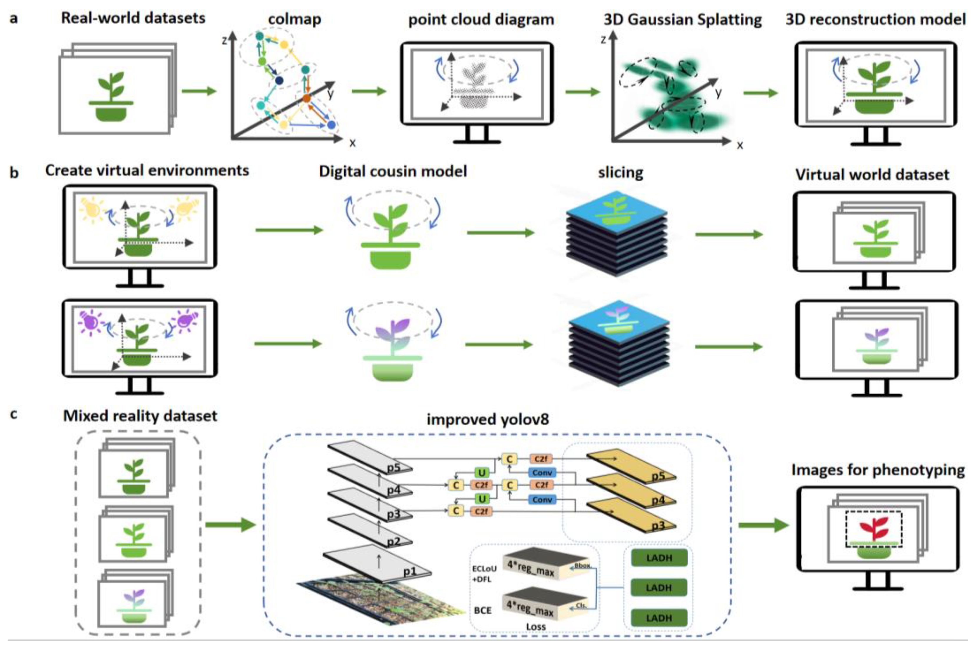
Figure 2.
Converting seedling images into sparse 3D point clouds using COLMAP.
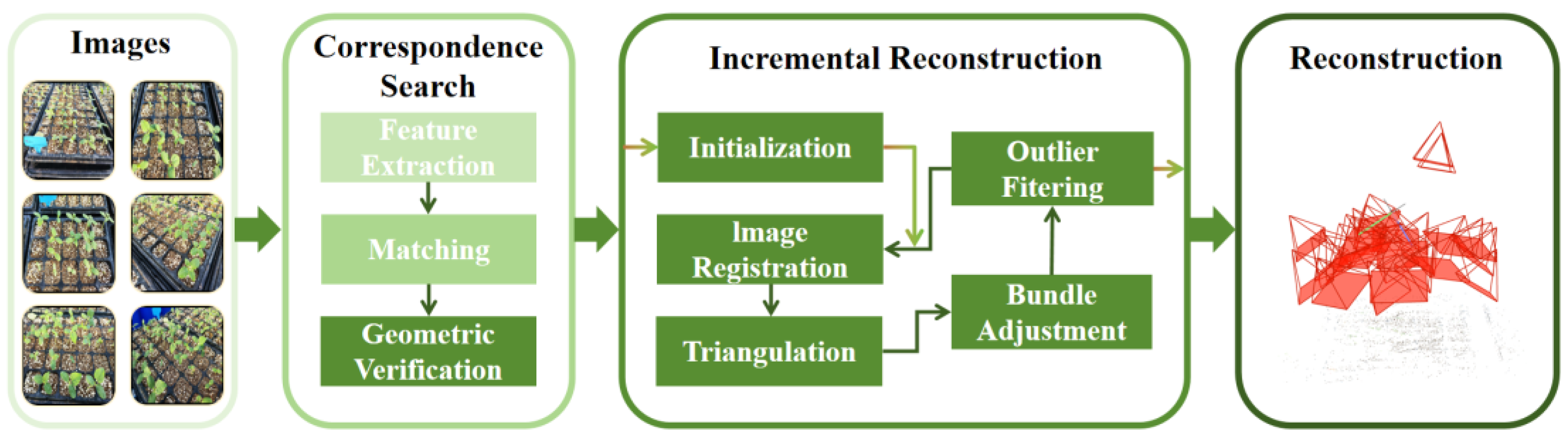
Figure 3.
Rendering of sparse 3D point clouds generated by COLMAP using 3D Gaussian Splatting to obtain high-quality seedling models.
Figure 3.
Rendering of sparse 3D point clouds generated by COLMAP using 3D Gaussian Splatting to obtain high-quality seedling models.
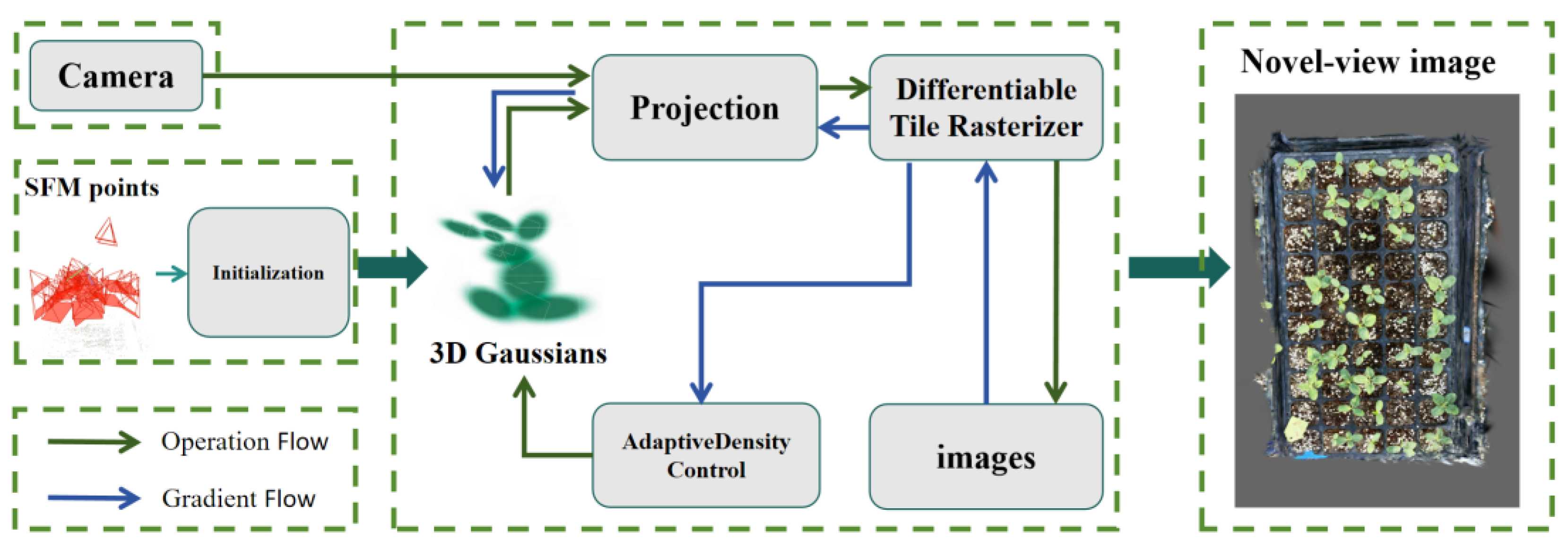
Figure 4.
LADH structure in the improved YOLOv8 network structure.
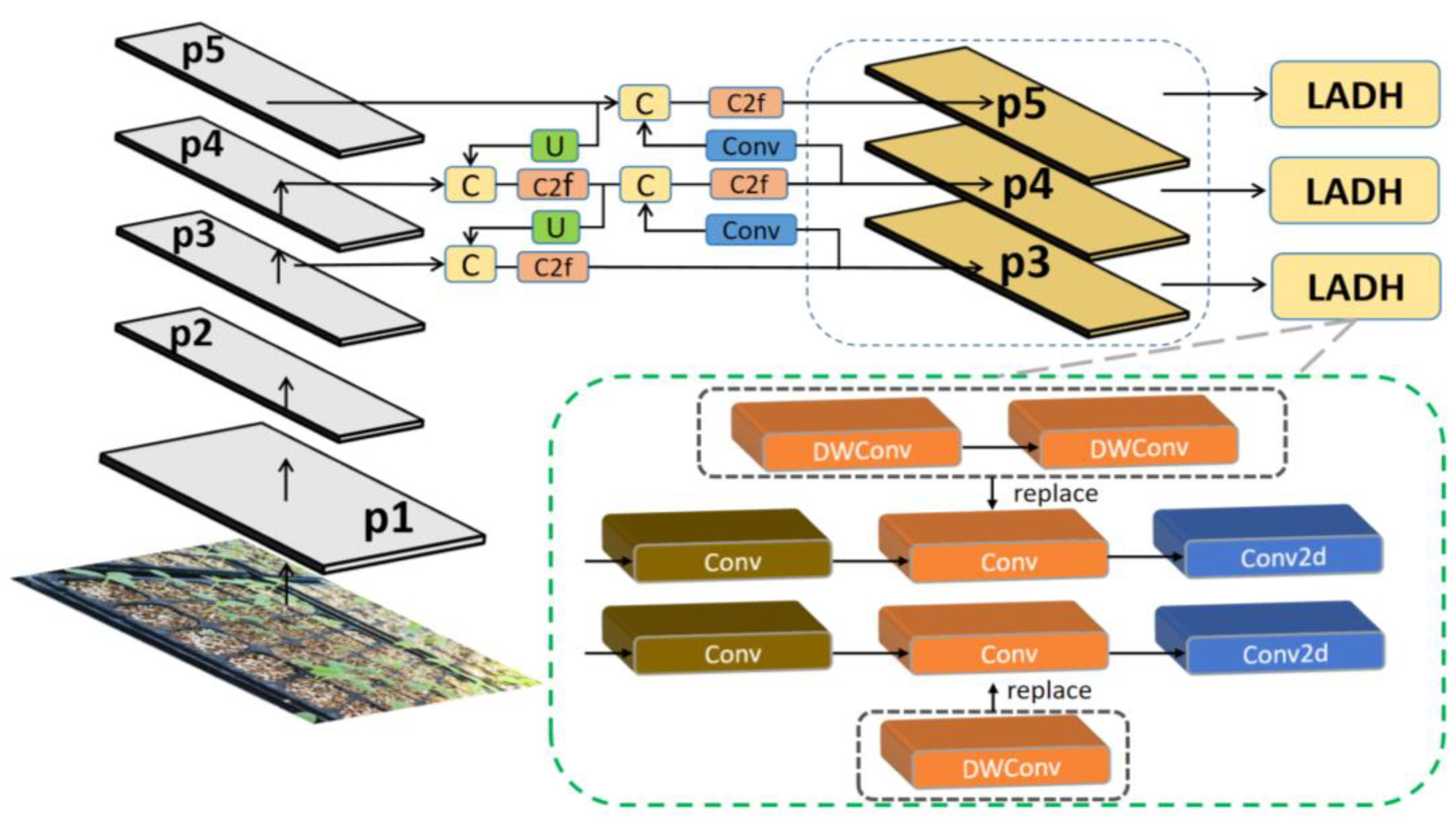
Figure 5.
SPPELAN structure in the improved YOLOv8 network structure.
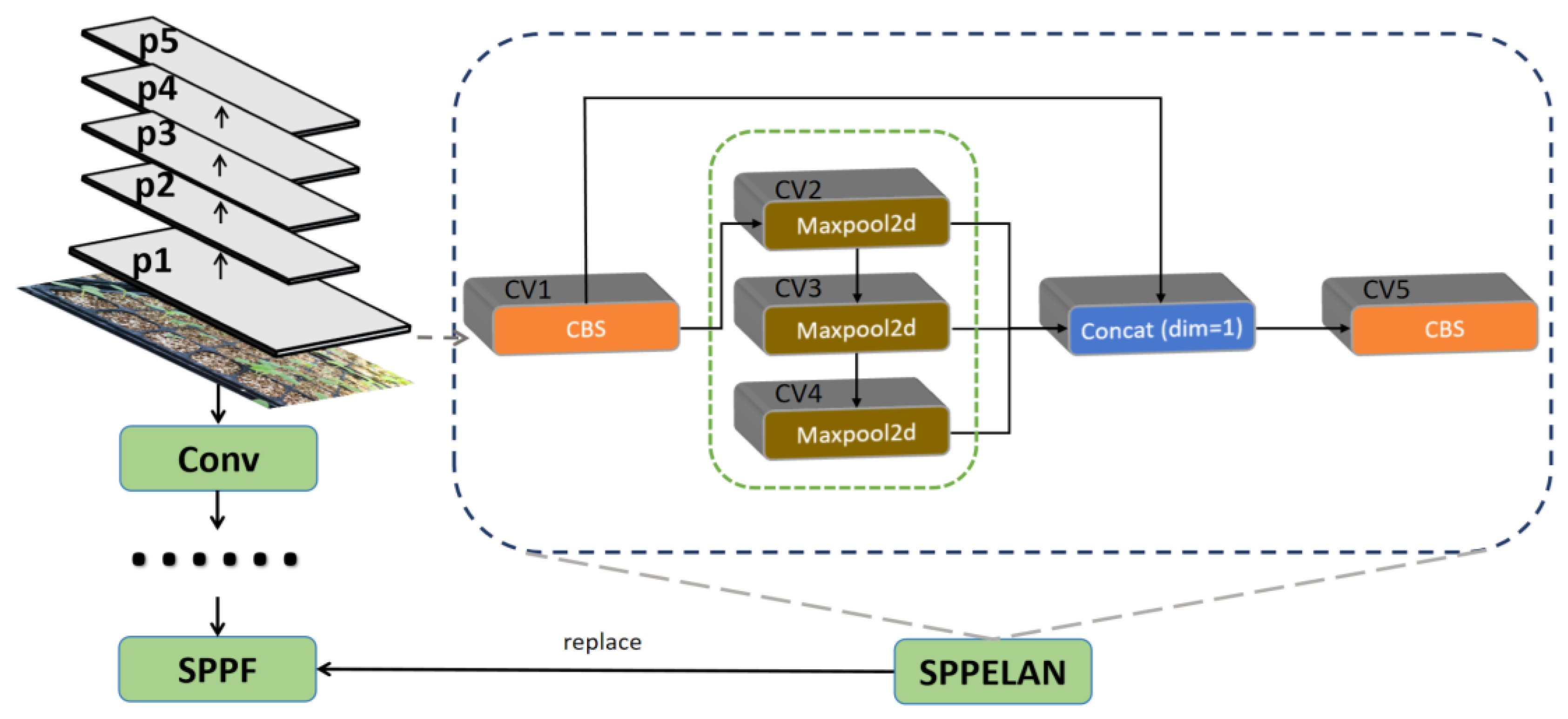
Figure 6.
Demonstration of our dataset in different light conditions. (a) Representative diagram of the model under strong light conditions; (b) Representative diagram of the model under medium light conditions; (c) Representative diagram of the model under Violet light conditions.
Figure 6.
Demonstration of our dataset in different light conditions. (a) Representative diagram of the model under strong light conditions; (b) Representative diagram of the model under medium light conditions; (c) Representative diagram of the model under Violet light conditions.
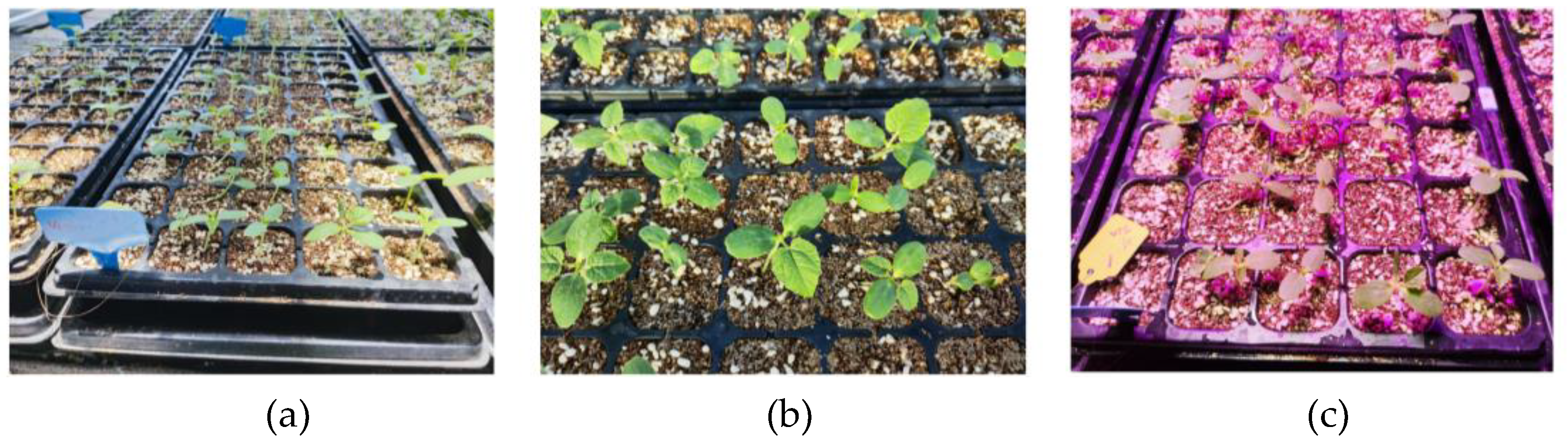
Figure 7.
Novel-view image rendered from 3D Gaussian Splatting——D1 Strong light.
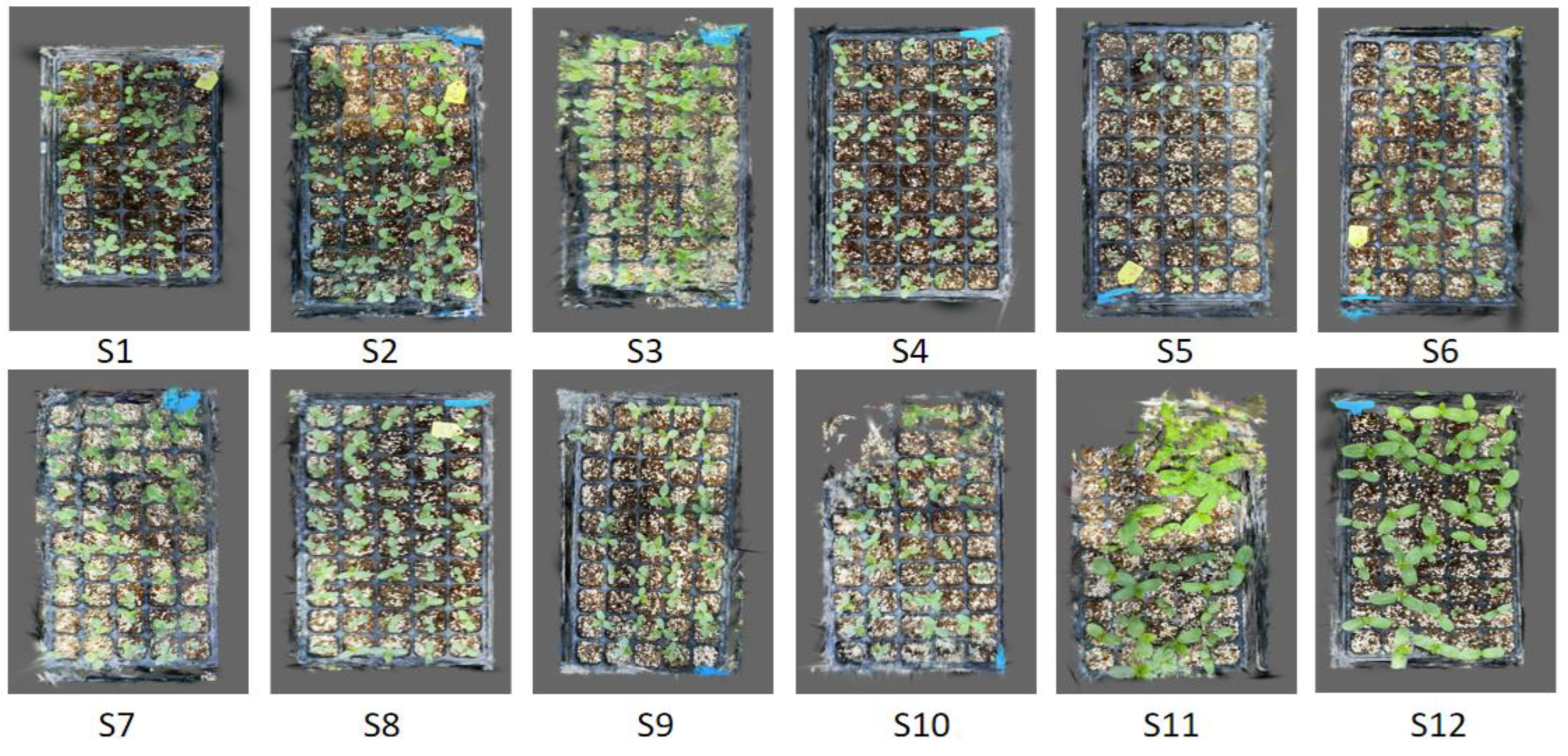
Figure 8.
Novel-view image rendered from 3D Gaussian Splatting——D2 Medium light.
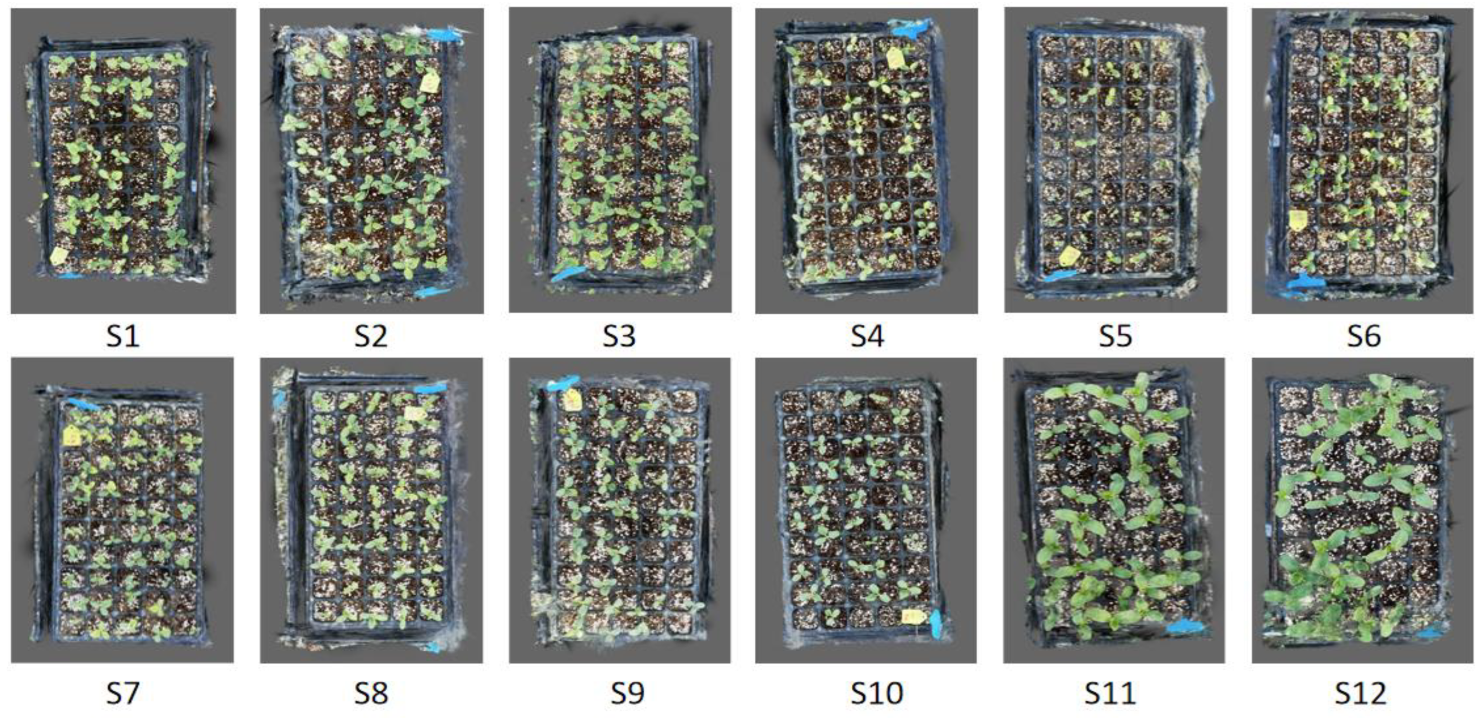
Figure 9.
Novel-view image rendered from 3D Gaussian Splatting——D3 Violet light.
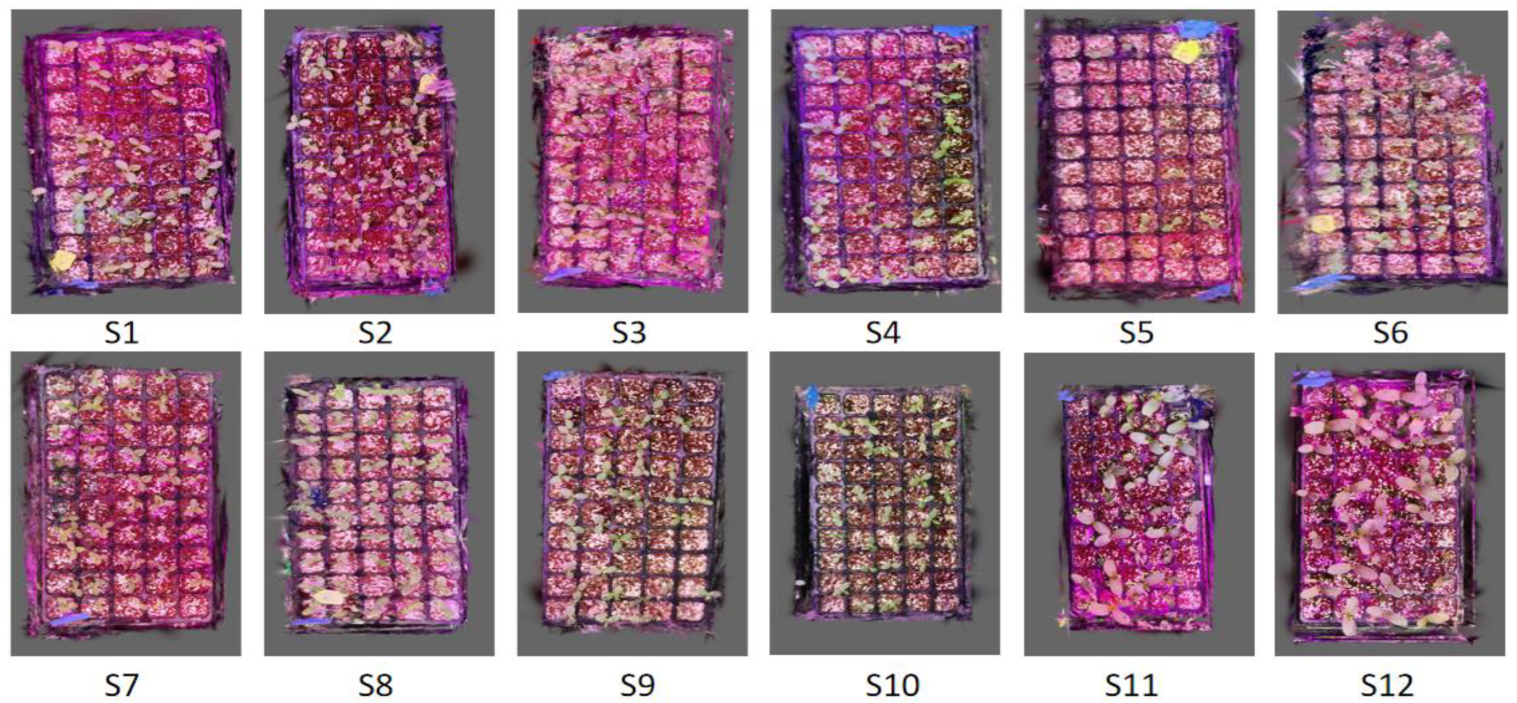
Figure 10.
Visualized waterfall plots of 3D Gaussian Splatting and Instant-NGP reconstructing model parameters in three lighting scenarios. (a) Comparison of Instant NGP, 3D Gaussian Splatting trained 7000 times and 30,000 times under strong light; (b) Comparison of Instant NGP, 3D Gaussian Splatting trained 7000 times and 30,000 times under medium light; (c) Comparison of Instant NGP, 3D Gaussian Splatting trained 7000 times and 30,000 times under violet light.
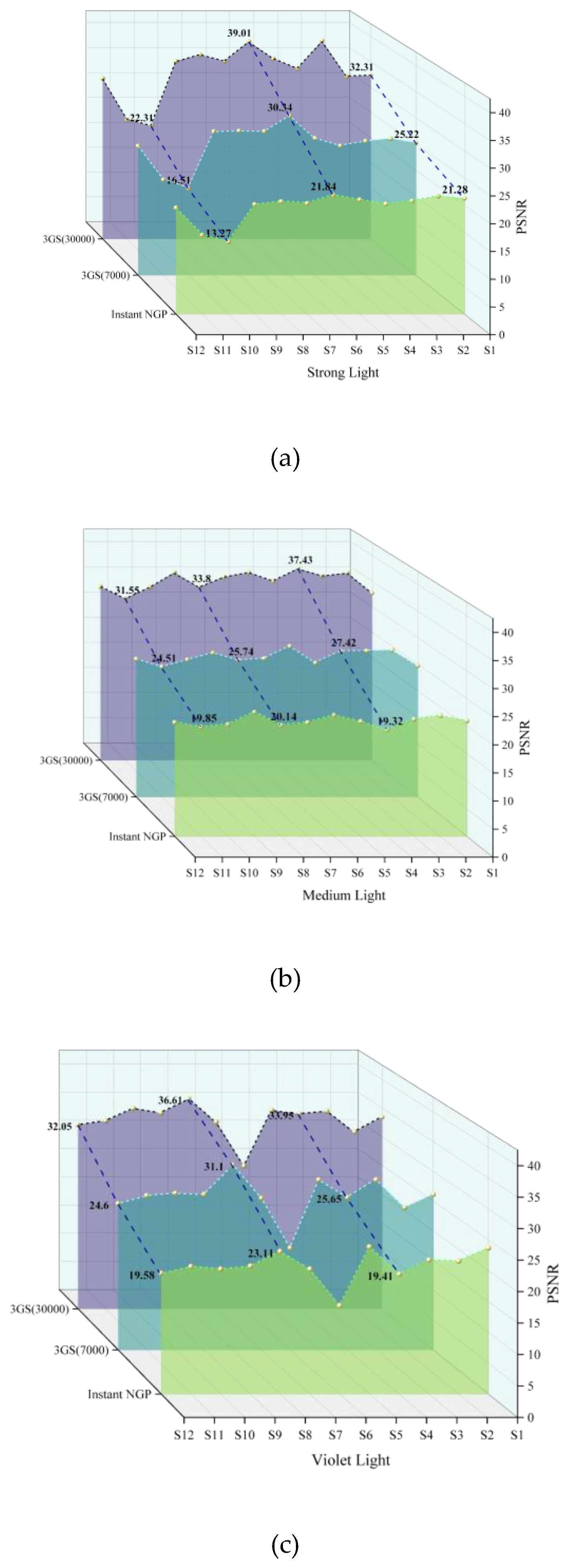
Figure 11.
Comparison of 3D Gaussian Splatting and Instant-NGP in details on the model surface.
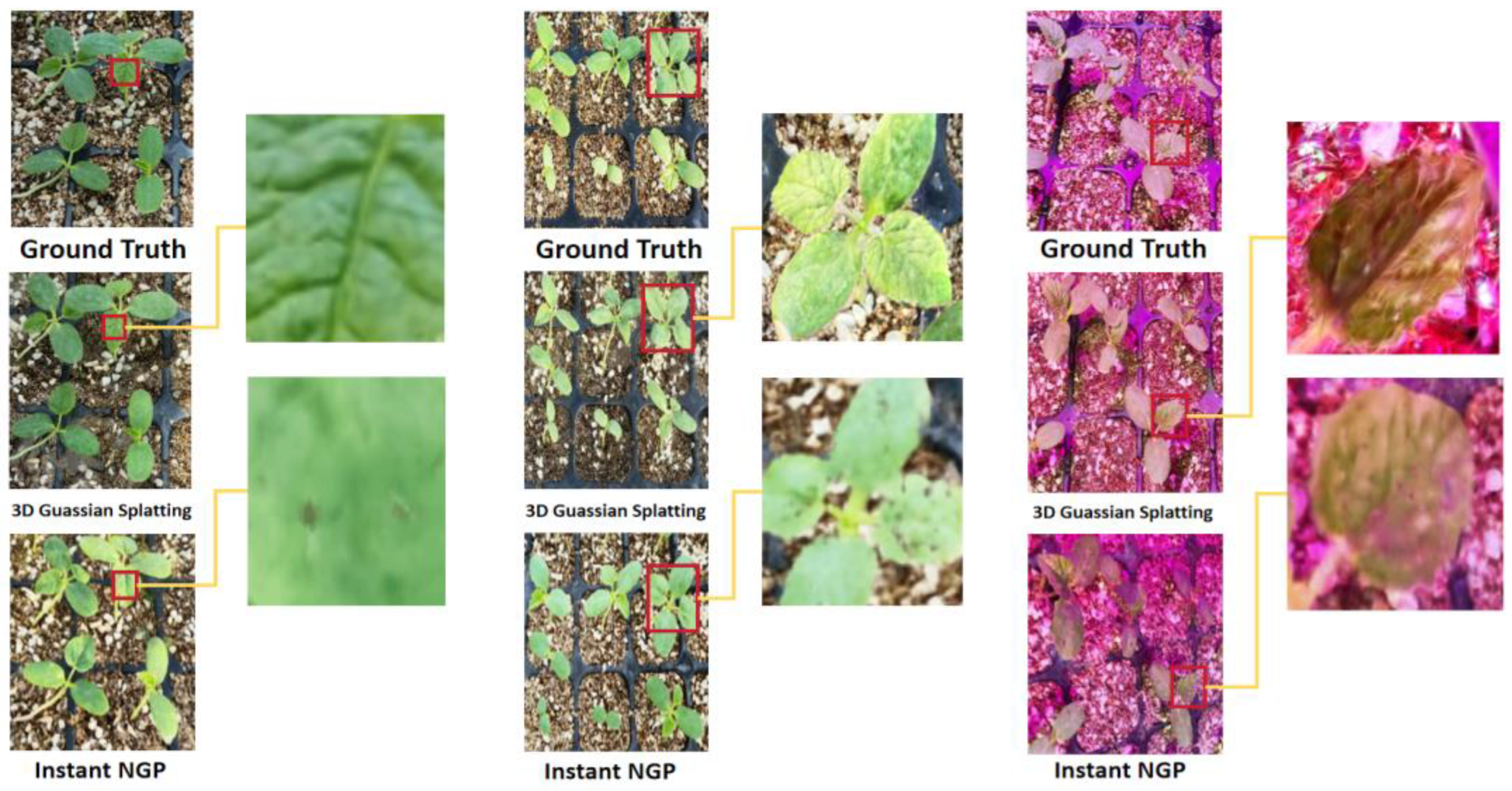
Figure 12.
3D modelling with defects. (a) Missing models due to shooting randomness in medium lighting; (b) Missing models due to shooting randomness in strong lighting; (c) Missing models due to shooting randomness in violet lighting.
Figure 12.
3D modelling with defects. (a) Missing models due to shooting randomness in medium lighting; (b) Missing models due to shooting randomness in strong lighting; (c) Missing models due to shooting randomness in violet lighting.
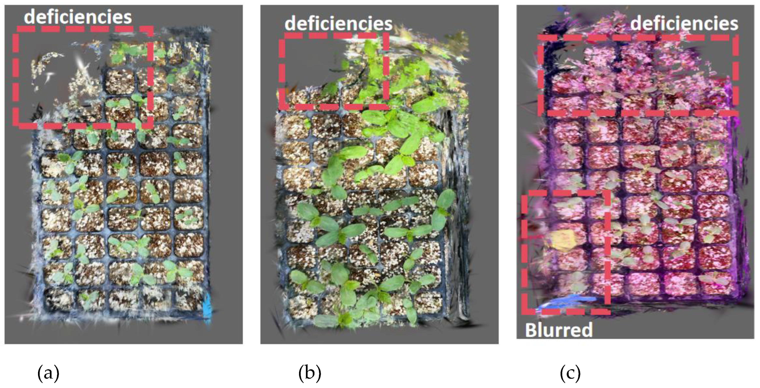
Figure 13.
Comparison chart of actual detection results. (a) Graph of test results for YOLOv8; (b) Graph of test results for ours.
Figure 13.
Comparison chart of actual detection results. (a) Graph of test results for YOLOv8; (b) Graph of test results for ours.
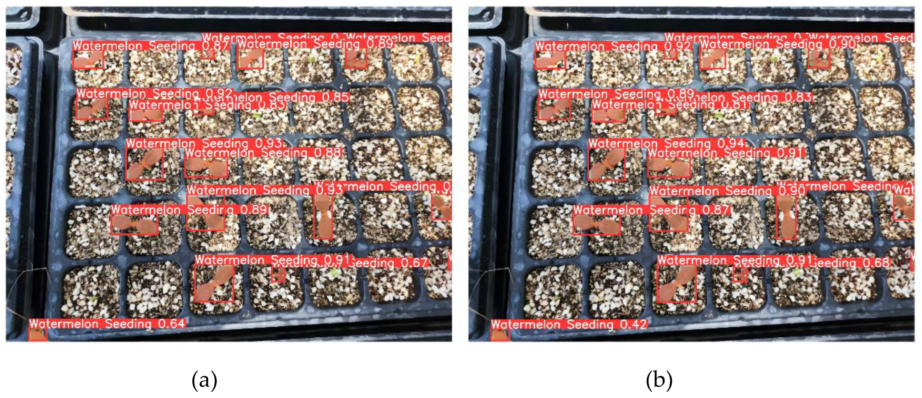

Table 1.
Mobile device parameters.
| Parameter | Value |
|---|---|
| Resolution | 4624*3472 |
| Flash bulb | none |
| Storage space | 256GB |
| Weight | 210g |
| Battery capacity | 4700mAh |
Table 2.
D1 group training results (Strong light).
| DATASET | 3D GAUSSIAN SPLATTING(Strong light) | Instant NGP(Strong light) | ||||
|---|---|---|---|---|---|---|
| Time-7000 | PSNR-7000 | Time-30000 | PSNR-30000 | Time | PSNR | |
| S1 | 5.38min | 25.22 | 30.03min | 32.31 | 3.05min | 21.28 |
| S2 | 5.87min | 26.02 | 27.65min | 32.09 | 3.13min | 21.65 |
| S3 | 6.00min | 25.55 | 30.85min | 39.17 | 3.82min | 20.77 |
| S4 | 5.45min | 24.64 | 31.52min | 33.67 | 3.18min | 20.25 |
| S5 | 6.15min | 26.11 | 29.38min | 35.61 | 3.65min | 21.02 |
| S6 | 5.77min | 30.34 | 29.85min | 39.01 | 3.45min | 21.84 |
| S7 | 5.82min | 27.40 | 27.98min | 35.11 | 3.58min | 20.34 |
| S8 | 6.03min | 27.49 | 29.62min | 36.37 | 3.98min | 20.67 |
| S9 | 5.35min | 27.40 | 27.55min | 35.11 | 3.25min | 20.14 |
| S10 | 5.67min | 16.51 | 22.87min | 22.31 | 3.33min | 13.27 |
| S11 | 6.35min | 18.20 | 24.65min | 23.56 | 4.11min | 14.54 |
| S12 | 5.82min | 24.63 | 28.45min | 31.68 | 3.87min | 19.51 |
Table 3.
D2 group training results (Medium light).
| DATASET | 3D GAUSSIAN SPLATTING(Medium light) | Instant NGP(Medium light) | ||||
|---|---|---|---|---|---|---|
| Time-7000 | PSNR-7000 | Time-30000 | PSNR-30000 | Time | PSNR | |
| S1 | 6.77min | 24.72 | 31.55min | 32.64 | 3.87min | 20.96 |
| S2 | 7.02min | 27.65 | 33.25min | 36.57 | 4.30min | 21.88 |
| S3 | 5.87min | 27.52 | 30.62min | 35.97 | 3.55min | 21.24 |
| S4 | 6.55min | 27.42 | 32.45min | 37.43 | 3.67min | 19.32 |
| S5 | 6.52min | 25.23 | 34.21min | 34.97 | 3.82min | 20.85 |
| S6 | 6.32min | 28.37 | 33.30min | 36.65 | 3.58min | 21.98 |
| S7 | 6.45min | 26.07 | 33.75min | 35.78 | 3.45min | 20.65 |
| S8 | 6.77min | 25.74 | 32.25min | 33.80 | 3.13min | 20.14 |
| S9 | 5.98min | 27.12 | 29.82min | 36.64 | 3.85min | 22.54 |
| S10 | 6.77min | 25.84 | 34.52min | 33.75 | 4.03min | 20.32 |
| S11 | 6.21min | 24.51 | 30.85min | 31.55 | 4.48min | 19.85 |
| S12 | 6.13min | 25.98 | 29.77min | 33.87 | 3.70min | 20.66 |
Table 4.
D3 group training results (Violet light).
| DATASET | 3D GAUSSIAN SPLATTING(Violet light) | Instant NGP(Violet light) | ||||
|---|---|---|---|---|---|---|
| Time-7000 | PSNR-7000 | Time-30000 | PSNR-30000 | Time | PSNR | |
| S1 | 6.18min | 26.16 | 29.85min | 33.43 | 4.14min | 23.66 |
| S2 | 5.93min | 23.94 | 30.03min | 30.85 | 3.35min | 21.54 |
| S3 | 6.10min | 28.60 | 23.58min | 34.47 | 3.77min | 21.72 |
| S4 | 6.21min | 25.65 | 32.65min | 33.95 | 3.68min | 19.41 |
| S5 | 6.33min | 28.61 | 23.68min | 34.62 | 4.32min | 23.85 |
| S6 | 6.17min | 17.15 | 23.45min | 24.90 | 3.70min | 14.32 |
| S7 | 5.85min | 25.53 | 28.70min | 32.55 | 3.82min | 20.25 |
| S8 | 6.11min | 31.10 | 23.48min | 36.61 | 3.97min | 23.11 |
| S9 | 5.87min | 26.16 | 28.63min | 34.14 | 3.35min | 20.74 |
| S10 | 5.97min | 26.34 | 23.77min | 34.93 | 3.55min | 20.25 |
| S11 | 6.30min | 25.96 | 26.97min | 32.76 | 3.82min | 20.66 |
| S12 | 6.18min | 24.60 | 27.80min | 32.05 | 3.80min | 19.58 |
Table 5.
Comparison with other methods.
| MODELS | BOX-MAP50 | MASK-MAP50 | LOSS | EPOCH |
|---|---|---|---|---|
| YOLOV5N-SEG | 0.895 | 0.909 | 0.855 | 201 |
| YOLOV8N-SEG | 0.907 | 0.909 | 0.765 | 370 |
| OURS | 0.910 | 0.913 | 0.616 | 254 |
Table 6.
Ablation experiments when LADH, Focaler-ECIOU, and SPPELAN are applied to Baseline.
| Methods | LADH | Focaler-ECIoU | SPPLAN | mAP50(B) | mAP50(M) | Epoch | Loss | GFLOPS |
|---|---|---|---|---|---|---|---|---|
| Baseline | × | × | × | 0.907 | 0.909 | 370 | 0.765 | 12.0 |
| LADH | √ | × | × | 0.906 | 0.908 | 201 | 0.854 | 11.6 |
| LADH+ Focaler-ECIoU | √ | √ | × | 0.907 | 0.913 | 181 | 0.667 | 11.6 |
| LADH+ Focaler-ECIoU +SPPELAN | √ | √ | √ | 0.910 | 0.913 | 254 | 0.616 | 11.1 |
Disclaimer/Publisher’s Note: The statements, opinions and data contained in all publications are solely those of the individual author(s) and contributor(s) and not of MDPI and/or the editor(s). MDPI and/or the editor(s) disclaim responsibility for any injury to people or property resulting from any ideas, methods, instructions or products referred to in the content. |
© 2024 by the authors. Licensee MDPI, Basel, Switzerland. This article is an open access article distributed under the terms and conditions of the Creative Commons Attribution (CC BY) license (http://creativecommons.org/licenses/by/4.0/).
Copyright: This open access article is published under a Creative Commons CC BY 4.0 license, which permit the free download, distribution, and reuse, provided that the author and preprint are cited in any reuse.


