
Submitted:
20 January 2026
Posted:
21 January 2026
You are already at the latest version
Abstract
Gravitational fingering often occurs for water flow in the vadose zone and accurate modeling of this important flow process remains a significant scientific challenge. This paper presents the latest theoretical developments of the optimality-based Active Region Model (ARM), a macroscopic framework developed for describing gravitational fingering flow in the vadose zone. ARM divides the soil into active (fingering) and in-active regions, introducing a relationship between water flux and hydraulic gradient derived from the principle of optimality that the system self-organizes to maximize water flow conductivity. Unlike traditional models, ARM’s hydraulic conductivity de-pends on both capillary pressure or water saturation and water flux, reflecting the un-stable nature of fingering flow. The paper provides an updated mathematical derivation of ARM relationships using calculus of variations and extends ARM to account for small water flux in the non-fingering zone, resulting in a dual-flow field model. These new developments should make ARM more rigorous and realistic for field-scale applications.
Keywords:
fingering flow
; preferential flow
; soil water dynamics
; vadose zone
; soil physics
; critical zone
1. Introduction
The vadose zone (the unsaturated zone) lies between the land surface and the groundwater table. It plays a crucial role in controlling the movement of nutrients and contaminants to groundwater, as well as in groundwater recharge. As an integral part of the critical zone, the Earth's outer layer where rock, soil, water, air, and living organisms interact, the vadose zone significantly influences how climate change affects the overall health of ecosystems. Central to all these processes is the movement of water within the vadose zone.
Downward water flow in vadose zone is often associated with so-called preferential flow that is non-uniform, can bypass significant portion of soils, and thus results in rapid water flow and solute transport from the ground surface to water table for a given water flux at the ground surface [1]. Two primary processes drive this phenomenon. The first involves macropores that facilitate swift water movement that is not in the hydraulic equilibrium with surrounding soil matrix [2,3]. The second process is gravitational fingering, which arises from instabilities at the wetting front during infiltration, leading to finger-like patterns of flow [4,5,6,7]. In real-world settings, both mechanisms may operate simultaneously, complicating the prediction and modeling of preferential flow. Developing robust and theoretically sound models to accurately represent these complex flow dynamics remains a significant scientific challenge [8].
This work focuses on gravitational fingering flow in homogeneous unsaturated soils. The traditional theory for water flow in unsaturated soil is valid under the local equilibrium condition. A discussion of local equilibrium concept within the context of thermodynamics can be found in Glansdorff and Prigogine [9]. A practical definition of local equilibrium, within a context of numerical modeling, is that capillary pressure and water saturation are relatively uniform within a numerical grid block such that the state of water distribution within the block can be adequately represented by average water saturation there. This is the fundamental reason why relative permeability is only a function of capillary pressure or water saturation under local equilibrium conditions. However, this assumption breaks down when fingering flow occurs within a grid block, necessitating a different theoretical framework to accurately describe the water flow process. While much research has focused on preferential flow related to macropores, there has been relatively limited progress in developing a macroscopic theory or modeling approach for fingering flow.
The optimality-based ARM has been developed as a macroscopic theory for fingering flow in the vadose zone [7,10,11]. It divides the representative elementary volume into two distinct zones: active and inactive regions. The active region is characterized by fingering water flow, while the inactive region remains bypassed. The macroscopic relation between soil water flux and the hydraulic gradient was derived from the principle of optimality that soil water flow pattern is self-organized to maximize the flow conductivity [7,10,11]. Optimality is deeply rooted in non-linear thermodynamics. Unlike the traditional theory for water flow, where conductivity is a function of capillary pressure or water saturation, hydraulic conductivity for fingering flow in ARM is also a power function of water flux.
The development of ARM was motivated by the demonstrated effectiveness of the Active Fracture Model (AFM) in simulating macroscopic water flow through the unsaturated zone at Yucca Mountain, where dense fractures can be treated as a continuum for water movement [7,12]. Since its inception, ARM has undergone extensive verification from multiple perspectives. The optimality-based ARM has been shown to align mathematically with the fractal characteristics of fingering flow patterns commonly observed in practice [11,13]. Its relationship between the fingering flow fraction and water flux matches well with laboratory observations [14]. Most recently, Liu et al. [15] demonstrated that ARM can reliably reproduce field results from dye infiltration experiments using only laboratory-measured soil properties, without the need for additional tunable parameters. (The related ARM simulator is available from https://github.com/blander996/Active-Region-Model.git.) This highlights ARM’s robustness and practicality for modeling fingering flow dynamics in natural soils. ARM has also been found useful for modeling field scale flow and transport in vadose zone by Sheng et al. [16], Engstrom and Liu [17] and Chen et al. [18], although further field evaluations of AEM under diverse conditions are warranted. Additionally, the optimality principle underlying ARM has been successfully applied to predict density-driven fingering transport rates (convective flux) for CO₂ storage in saline aquifers [19]. The success of the optimality principle in describing fingering phenomena across distinct contexts further strengthens validity of ARM’s physics foundation.
This study presents two latest theoretical developments of ARM. The mathematical derivation of the ARM relationship has been continuously updated and refined while the final results remain unchanged, because certain approximation is needed in the derivation [7,10,11]. For the completeness and transparency, this short communication provides the more rigorous derivation of ARM’s relationship between water flux and hydraulic gradient based on the optimality. Also, in the previous studies related to ARM, water is considered immobile within the non-fingering zone. In some field-scale contexts, the non-fingering flow zone, however, does carry a small flux, albeit much slower than in the fingers. Thus, ARM is further extended in this study to cases in which water flow is allowed to occur in the non-fingering flow zone. Hopefully, these new developments provide a more general and realistic ARM framework for modeling macroscopic fingering flow in the vadose zone.
2. The Relationship between Water Flux and Hydraulic Gradient
Modeling vadose-zone flow requires relating water flux to the hydraulic gradient. Under local equilibrium, this relationship is given by the Darcy–Buckingham law. Because Darcy–Buckingham law fails at macroscale when fingering occurs, deriving a macroscopic relation for the ARM requires an additional principle. This section derives the relation using the optimality principle: water in unsaturated soils organizes its flow to minimize global resistance or maximize conductivity.
Following the common practice for determining large-scale flow parameters (e.g., [20]), we focus on the steady-state flow process, given that this work emphasizes the fully developed fingering flow. The steady-state water flow equation on the large scale (Figure 1) for a homogeneous and isotropic porous medium is given as
where x and y are the two horizontal coordinate axes, z is the vertical axis, and qx, qy and qz are large-scale Darcy flux along x, y and z directions, respectively.
The expression for energy expenditure rate needs to be derived for applying the optimality principle. The energy of unit weight of liquid water (or hydraulic head) in a porous medium, E, is given by
where h is the average capillary pressure head within the fingering flow zone (Figure 1). For a unit volume of porous medium, the energy expenditure rate is given as
Combining Equations.(1) and (3) yields
Therefore, the rate of water energy loss is represented by a product of water flux and energy gradient or hydraulic gradient.
Following Liu [7,10,11], we assume that the mathematical form of Darcy-Buckingham law is still applicable to fingering process at the large scale:
The major difference between Liu [7,10,11] and the traditional unsaturated flow theory is the expression for hydraulic conductivity (K). Conventionally, K is a function of water saturation or capillary pressure only in the Darcy-Buckingham law. This is a direct consequence of the local equilibrium assumption, which is not valid for modeling fingering flow on a large scale. Local equilibrium refers to the existence of thermodynamic equilibrium within a representative elementary volume (REV). (A numerical grid block size should be larger than or equal to REV and different sizes of REV may exist at different scales [21].) In other words, temperature, fluid saturation and capillary pressure are always uniformly distributed within REV under local equilibrium conditions (e.g., the local scale shown in Figure 1). In contrast, non-equilibrium means that thermodynamic equilibrium does not exist within REV containing sub-grid fingering (e.g., the large-scale shown in Figure 1). Thus, the water distribution within the large-scale REV (Figure 1) cannot be uniquely determined by water saturation or capillary pressure alone. ARM is a continuum model associated with the large-scale REV (Figure 1). In this case, additional large-scale variables are needed to accurately determine the state of sub-grid water distribution. Water flux is a logical choice because it is highly relevant to the fingering flow process. Following Liu [7,10,11], we use the square of the energy gradient as the additional variable to determine the large-scale conductivity for mathematical convenience. This is equivalent to the use of water flux because water flux and the energy gradient are related to each other (Equation (5)). Here, the large-scale hydraulic conductivity is given by
where Ks is saturated hydraulic conductivity and the square of the energy gradient is defined by
Based on Equations (4), (5) and (7), we can write the total energy expenditure rate for the whole flow domain as
The optimality principle is used to derive the explicit relationship between K, h, and (Equation (6)). Note that is always negative because gained water energy is considered positive in this study. When applying the optimality principle regarding the minimization of global flow resistance (or the maximum conductivity), absolute value of the total energy expenditure rate can either be minimized or maximized, depending on the boundary conditions. For fixed energy values at the boundaries, the minimum flow resistance allows the maximum water flux, resulting in the maximum absolute value of the energy expenditure rate or the maximum entropy production under isothermal conditions. Conversely, for fixed flux values at the boundaries, the minimum flow resistance leads to the minimum absolute value of the energy gradient along the flow path, resulting in the minimum absolute value of the energy expenditure rate as well. These outcomes are direct results of the definition of the energy expenditure rate, which is the product of water flux and energy gradient. Here, we use boundary conditions with fixed energy values, which, as shown later, enable the derivation of mathematically tractable results. Intuitively, optimal conductivity should not depend on the specific boundary conditions used in the derivation.
The calculus of variations is employed here to address the extremum problems of Equation (8). While we refer to relevant mathematical books for detailed information on calculus of variations (e.g., [22]), some pertinent results are briefly presented here. Consider a functional (Iw) with an unknown function (w):
where function L is called the Lagrangian, and wx, w y, and wz are derivatives of w with respect to x, y, and z, respectively. When Iw reaches its extrema, the Euler equation [22] can be used for determining the unknown function w:
Note that the Euler equation above holds only when w has fixed values or satisfies the following condition at boundaries:
Equations (9) and (10) are applied to a functional with one unknown function. When there are more than one unknown functions, Equation (10) will apply to each one of these functions (e.g., [22]).
The following Lagrangian function is obtained from Equation (8):
The second term on the right-hand side is a constraint from Equation (7) and the Lagrange multiplier is a function here. The constraint related to the water flow equation (Equation (1)) is not included in Equation (12) and will be delt with later.
Since the Lagrangian function does not directly involve the derivative of with respect to x, y and z, satisfies Equation (11). Then Equation (10) can be applicable when replacing w with . Inserting Equation (12) into Equation (11) gives:
Here, we consider a boundary condition with E values being fixed at boundaries. Thus, Equation (10) is applicable when replacing w with E. Inserting Equation (12) into (10) and using Equations (13) and (1) yield:
Note that in the above equation was replaced by in Liu [7,11]. Equation (14) is mathematically more accurate.
If the term on the right-hand side of Equation (14) is zero or negligible for gravity-dominant water flow, an analytical relationship for the large-scale hydraulic conductivity can be obtained [7,11]. Change in E largely results from change in z while h only contributes to a relatively small portion of changes in E, which is the nature of gravity dominated water flow that is mainly along the vertical direction. Specifically in Equation (2), E is the summation of z and h; the former is the contribution from gravity and the latter from capillary force which is weak for gravity dominated fingering flow. Considering that K is related to h and not to z (Equation (6)), its relationship with E herein should be weak and thus the derivative of K with respect to E is approximately negligible. To illustrate this point with a special case, consider two close elevations in Figure 1 where the capillary pressure heads and fractions of fingering flow zone are the same at the two locations. Here, E will be different at these two locations because of the z difference (Equation (2)), but K remains the same given that it only depends on h and the fraction of fingering flow zone, as will be discussed later. Thus, holds for this special case because the change in E does not result in the change in K. Nevertheless, should be considered an approximation for a general case. Validity of considering K to be a weak function of E is further verified by excellent agreements between the related theoretical results derived from it and experimental observations [11,14,15].
When the term on the right-hand side of Equation (14) drops, the equation becomes
Note that Equation (1) can be rewritten as
Equation (15) outlines the partial differential equation that K must satisfy according to the optimality principle. However, the derivation of Equation (15) does not consider the constraints imposed by the water flow equation (Equation (1) or (16)), as previously mentioned. By comparing Equations (15) and (16), it becomes evident that the water flow equation (Equation (16)) is also satisfied when
where is a constant.
Following Liu [7], we approximately rewrite the mathematical form of K with
where and are functions of h and S*, respectively. Inserting Equation (18) into Equation (17) gives
According to Equation (5), the above equation can be further rewritten as
where q is the magnitude of water flux defined by
Then relationship of large-scale hydraulic conductivity is obtained by inserting Equation (20) into Equation (18):
where Fh is a function of h and a is a constant. The term in Equation (22) is considered relative permeability on the local scale (Figure 1) simply because it is only a function of h or the capillary pressure head in fingering flow zone. The power function term represents the fraction of fingering flow zone in the cross section normal to the flux direction [7,10,11]:
The parameter a value seems to be in a narrow range (0.4 to 0.5) for different types of soils according to the data collected from both laboratory experiments and field tests [11,14,15].
The large-scale hydraulic conductivity being a function of flux, as shown in Equation (22), aligns with the behavior of other unstable flow processes, such as turbulent flow. Liu [7] compared Equation (22) to the expression of water viscosity in hydrodynamics literature, considering conductivity and viscosity as conceptual analogues. For comparison purposes, laminar water flow and turbulent flow in hydrodynamics correspond to uniform flow (or non-fingering flow) in unsaturated soils and fingering flow, respectively. For the uniform flow in unsaturated soils, hydraulic conductivity is solely a function of water saturation, which is like water viscosity in laminar flow that is a sole property of water, independent of water velocity. However, in turbulent flow, the apparent viscosity is related to the Reynolds number (Re), which is a function of water velocity. Therefore, it is not surprising that conductivity for fingering flow in the vadose zone depends on water flux as well, as both fingering flow in unsaturated soils and turbulent flow in hydrodynamics belong to the same flow regime: unstable flow. Additionally, just as different constitutive models exist for laminar and turbulent flow regimes in hydrodynamics, we need to develop a theoretical framework for large-scale fingering flow, alongside the framework for uniform flow (Darcy-Buckingham law), to fully describe water flow in all regimes in the vadose zone. This will be further discussed in the next section.
For a positive value of a, Equation (22) suggests that locations with high water fluxes will also have high conductivity values, thereby minimizing global flow resistance. This concept aligns with our everyday experiences. For instance, to optimize traffic transportation efficiency, highways are designed with more lanes in areas with high traffic flow. In this analogy, highway networks resemble fingering flow paths, with traffic flux and the number of lanes corresponding to water flux and hydraulic conductivity, respectively.
The final optimality-based relationship between soil water flux and energy or hydraulic gradient is obtained as follows by combining Equations (5) and (22):
where bold characters are vectors, f is given by Equation (23) and , identical to in Equation (22), represents local-scale water relative permeability and can be determined by the van Genuchten [23] equation with water saturation or capillary pressure in the fingering zone. Although the water flux term occurs on both sides of the equation, Equation (22) is convenient for use in practice and its physics meanings are also relatively easy to understand because f, the fraction of fingering flow zone, is explicitly present in the equation. This is especially useful for modeling solute transport with the ARM given that f is a key parameter for determining the pore velocity [17].
To avoid the flux term on the right hand of Equation (24), it can be rewritten as follows
where bold characters are again vectors. Note that for a = 0 (or f =1) Equation (25) is reduced to Darcy-Buckingham law. Although Equation (25) is mathematically identical to Equation (24), the relation between water flow patterns associated with gravitational fingering is more difficult to visualize from Equation (25). Nevertheless, one important implication from Equation (25) is that from a small scale to a large scale it is not enough to upscale flow parameters with mathematical forms of fundamental laws being assumed to be the same across scales. For example, at a local scale within a finger, Darcy-Buckingham law holds because of the existence of the local equilibrium at that scale. However, a different form of flux-gradient relationship (Equation (25)) needs to be used for a larger scale involving multiple fingers within each grid block.
3. A Model Generalization to the Dual-Flow Field
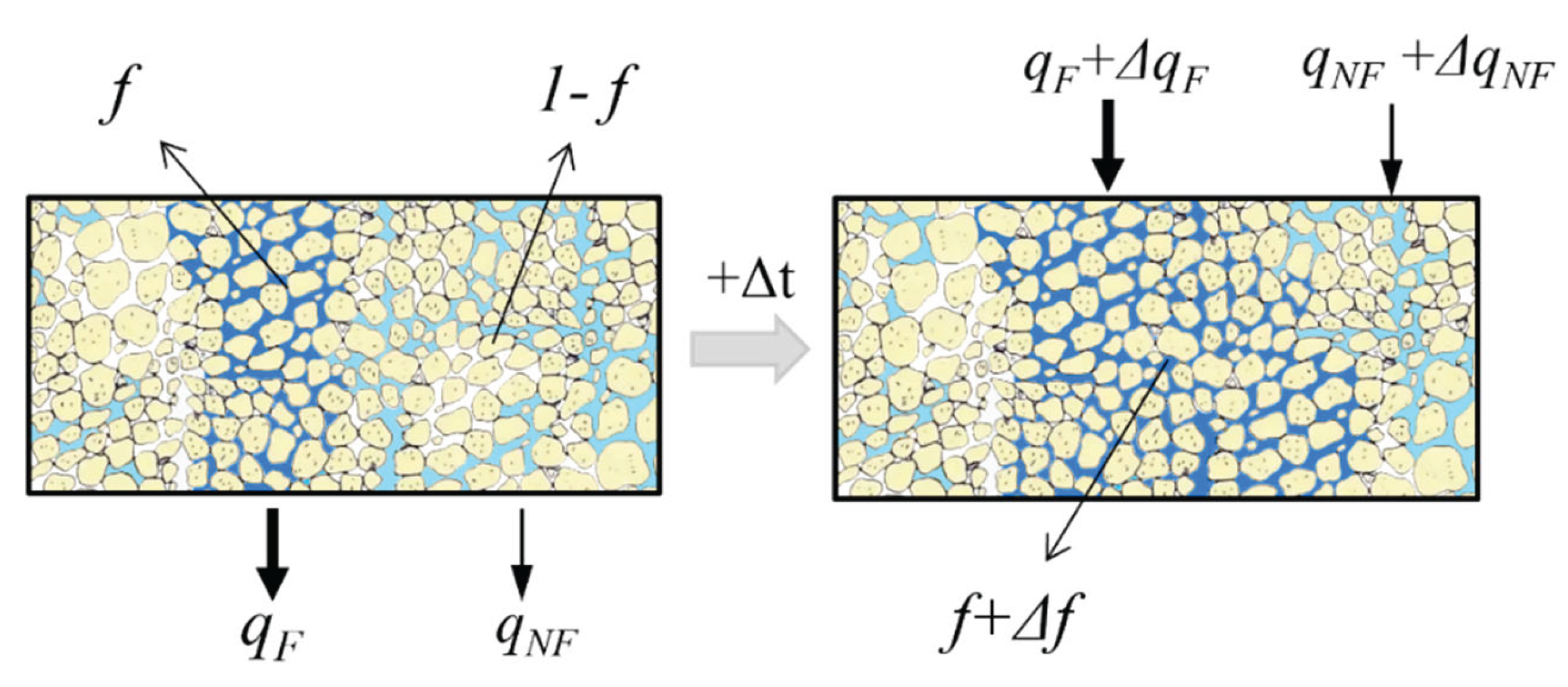
All the above discussions on modeling gravitational fingering flow in unsaturated soils with the optimality-based ARM assume that water is immobile within the non-fingering zone. In some field-scale contexts it does carry a small flux, albeit much slower than in the fingers. In a more general case, two flow fields coexist (Figure 2): the non-fingering zone with a relatively small water flux, governed by the Darcy-Buckingham law, and the fingering flow zone with a large water flux, described by the current theory based on the optimality [11]. This section develops a theoretical framework to capture both flows. Because vadose flow is predominantly vertical, we restrict attention to one-dimensional vertical flow.
Since soil water is considered incompressible under isothermal conditions, soil-water mass balance is reduced to its volume balance. The total soil-water volume balance equation is
where subscripts F and NF refer to fingering flow and non-fingering zones, respectively, is water content, t is time, z is again vertical coordinate with positive direction being downward, and q is the water flux defined here as the volumetric water flow rate divided by cross-sectional area of bulk soil including both fingering and non-fingering zones. Water fluxes corresponding to the two zones are, respectively, given by
and
where E is soil water energy (or hydraulic head), and the fraction of fingering flow zone is determined by
When there is no water flux in the non-fingering zone, is the same as the total water flux, and Equation (29) becomes identical to Equation (23). Also, note that and have the same relationship with local-scale water saturation. For example, if they are described by the van Genuchten [23] equation, they have the same values for the parameters in the equation because soils under consideration are homogeneous. However, at a given time, values for relative permeability and correspond to local-scale water saturations in fingering and non-fingering zones, respectively. Since the water saturation in the fingering flow zone is higher than that in the non-fingering zone, is larger than . Following the same line, is also different from . Clearly, these differences are reflection of the fact that fingering flow is inherently a nonequilibrium process.
Equation (26) describes the total soil-water volume balance involving both non-fingering and fingering zones. The following equation describes the volume balance specifically for the fingering flow zone:
The second term on the left-hand side of the above equation is related to the interaction between fingering flow zone and non-fingering zone (Figure 2). It results from the expansion (or shrinkage) of fingering flow zone to (or from) the non-fingering zone with original water content . The water volume associated with the original water content in the expanded domain is not directly from the fingering flow associated with and thus should be subtracted from the total volume in the fingering flow zone after the expansion in Equation (30).
Similarly, the volume balance equation for the non-fingering zone is given as follows:
Again, the second term on the left-hand side of the above equation is a result of the interaction between fingering flow zone and non-fingering zone. Equation (31) can be obtained by subtracting Equation (30) from Equation (26) and thus only two of these three volume balance equations (Equations (26), (30) and (31)) are independent.
To apply the generalized model for the dual-flow fields to soil water flow in homogeneous unsaturated soils, one needs to solve two of the three volume balance equations above, together with Equations (27), (28) and (29), under appropriate boundary and initial conditions. While the focus here is on the theoretical framework for the dual-flow field, we will leave to future studies the development of numerical algorithms for the generalized model and validations with experimental data.
4. Discussion
The Darcy–Buckingham law is applicable to water movement in unsaturated soils only when local equilibrium conditions are met. The local equilibrium breaks down when sub-grid fingering flow occurs. While studies have advanced our understanding of individual flow fingers at small scales, there remains a gap in macroscopic modeling frameworks for fingering flow [6]. Given current computational constraints, simulating large-scale fingering flow at the resolution (smaller than individual fingering width) required for direct application of the Darcy–Buckingham law is not yet practical. Therefore, robust macroscopic models are essential for addressing preferential flow in real-world scenarios. ARM has been developed for addressing this important issue.
When sub-grid fingering occurs, the average water saturation alone cannot uniquely define sub-grid water flow process. An additional constitutive relation is needed. Thus, optimality was introduced to deal with this in ARM. During the derivation of the relation between water flux and hydraulic gradient using calculus of variations, the mathematical difficulty is the approximation of term in Equation (14). Previously, this term was dropped based on the consideration that water in fingering zone is close to full saturation, which is realistic in many cases for unsaturated soil. This, however, cannot explain why the similar modeling framework is applicable to systems where fingering saturation is not very high, such as those studies related to unsaturated zone of Yucca Mountain [12]. In this work, we demonstrate that the term is indeed negligible simply because K is very weak function of E under gravity dominated flow conditions, including situations where fingering saturation may not be very high. Note that this new development does not change the final theoretical relation for ARM (Equation 22) but is critical to ensure the theoretical rigor of ARM framework.
In previous studies related to ARM, water is considered immobile within the non-fingering zone; the related ARM simulator is available from https://github.com/blander996/Active-Region-Model.git. In some field-scale contexts, non-fingering zone, however, does carry a small flux, albeit much slower than in the fingers. Thus, ARM is further extended in this study to cases in which water flow is allowed to occur in the non-fingering flow zone. This provides a more general and realistic ARM framework for modeling macroscopic fingering flow in the vadose zone, while we only focus on theoretical model development herein and leave the related numerical model development to future studies.
5. Conclusions
This paper presents the latest theoretical developments of the optimality-based Active Region Model (ARM), a macroscopic framework for describing gravitational fingering flow in the vadose zone. ARM divides the soil into active (fingering) and inactive regions, introducing a relationship between water flux and hydraulic gradient derived from the principle of optimality that the system self-organizes to maximize flow conductivity. Unlike traditional models, ARM’s hydraulic conductivity depends on both capillary pressure (or water saturation) and water flux, reflecting the unstable nature of fingering flow. The paper provides an updated mathematical derivation using calculus of variations and extends ARM to account for small water flux in the non-fingering zone, resulting in a dual-flow field model. These new developments should make ARM more general and realistic for field-scale applications.
Author Contributions
Conceptualization, H.L., Y.L., S. Z.; methodology, H.L., Y.L. and S. Z.; software, Y.L.; writing—original draft preparation, H.L.; writing—review and editing, Y.L., S. Z.; All authors have read and agreed to the published version of the manuscript.
Funding
This research received no external funding
Data Availability Statement
The data presented in this study is available on request from the authors.
Conflicts of Interest
The authors declare no conflicts of interest.
References
- Flury, M.; Flühler, H.; Jury, W.A.; Leuenberger, J. Susceptibility of soils to preferential flow of water: A field study. Water Resour. Res. 1994, 30, 1945–1954. [Google Scholar] [CrossRef]
- Beven, K.; Germann, P. Macropores and water flow in soils. Water Resour. Res. 1982, 18, 1311–1325. [Google Scholar] [CrossRef]
- Gerke, H.H.; van Genuchten, M.T. A dual-porosity model for simulating the preferential movement of water and solutes in structured porous media. Water Resour. Res. 1993, 29, 305–319. [Google Scholar] [CrossRef]
- Glass, R.J.; Steenhuis, T.S.; Parlarge, J.Y. Wetting front instability as a rapid and far-reaching hydrologic process in the vadose zone. J. Contam. Hydrol. 1988, 3, 207–226. [Google Scholar] [CrossRef]
- Wang, Z.; Feyen, J.; Elrick, D.E. Prediction of fingering in porous media. Water Resour. Res. 1998, 34, 2183–2190. [Google Scholar] [CrossRef]
- de Rooij, G.H. Modeling fingered flow of water in soils owing to wetting front instability: A review. J. Hydrol. 2000, 231–232, 277–294. [Google Scholar] [CrossRef]
- Liu, H.H. Fluid Flow in the Subsurface: History, Generalization and Applications of Physical Laws; Springer: Cham, Switzerland, 2017. [Google Scholar]
- Beven, K. A century of denial: Preferential and nonequilibrium water flow in soils, 1864–1984. Vadose Zone J. 2018, 17, 180153. [Google Scholar] [CrossRef]
- Glansdorff, P.; Prigogine, I. Thermodynamic theory of structure, stability and fluctuations; John Wiley & Sons Ltd: New York, 1971. [Google Scholar]
- Liu, H.H. A conductivity relationship for steady-state unsaturated flow processes under optimal flow conditions. Vadose Zone J. 2011, 10, 736–740. [Google Scholar] [CrossRef]
- Liu, H.H. The large-scale hydraulic conductivity for gravitational fingering flow in unsaturated homogenous porous media: A review and further discussion. Water 2022, 14(22). [Google Scholar] [CrossRef]
- Liu, H.H.; Doughty, C.; Bodvarsson, G.S. An active fracture model for unsaturated flow and transport in fractured rocks. Water Resour. Res. 1998, 34, 2633–2646. [Google Scholar] [CrossRef]
- Liu, H.H.; Zhang, R.; Bodvarsson, G.S. An active region model for capturing fractal flow patterns in unsaturated soils: Model development. J. Contam. Hydrol. 2005, 80, 18–30. [Google Scholar] [CrossRef] [PubMed]
- Liu, Y.; Zhang, S.; Liu, H.H. The relationship between fingering flow fraction and water flux in unsaturated soil at the laboratory scale. J. Hydrol. 2023, 622. [Google Scholar] [CrossRef]
- Liu, Y.; Zhang, S.; Liu, H.H.; Huang, Y.; Zhang, H.; Wang, G. An evaluation of the relationship between fingering flow fraction and water flux in natural field soil. J. Hydrol 2025, 661, 133783. [Google Scholar] [CrossRef]
- Sheng, F.; Wang, K.; Zhang, R.D.; Liu, H.H. Characterizing soil preferential flow using iodine–starch staining experiments and the active region model. J. Hydrol. 2009, 367, 115–124. [Google Scholar] [CrossRef]
- Engstrom, E.; Liu, H.H. Modeling bacterial attenuation in on-site wastewater treatment systems using the active region model and column-scale data. Environ. Earth Sci. 2015, 74, 4827–4837. [Google Scholar] [CrossRef]
- Chen, R.; Wang, Z.; Dhital, Y.P.; Zhang, X. A comparative evaluation of soil preferential flow of mulched drip irrigation cotton field in Xinjiang based on dyed image variability versus fractal characteristic parameter. Agricultural Water Management 2022, 269, 107722. [Google Scholar] [CrossRef]
- Liu, H.H.; Chen, J.; Jin, G.; AlYousef, Z. Determination of CO2 convective mixing flux in saline aquifers based on the optimality. Advances in Geo-Energy Research 2024, 13(2), 89–95. [Google Scholar] [CrossRef]
- Gelhar, L. Stochastic Subsurface Hydrology; Prentice Hall: Hoboken, NJ, USA, 1993. [Google Scholar]
- Bear, J. Modeling phenomena of flow and transport in porous media; Springer: Cham, Switzerland, 2018. [Google Scholar]
- Weinstock, R. Calculus of Variations with Applications to Physics and Engineering; Dover Publications, Inc.: New York, NY, USA, 1974. [Google Scholar]
- van Genuchten, M.T. A closed-form equation for predicting the hydraulic conductivity of unsaturated soils. Soil Sci. Soc. Am. J. 1980, 44, 892–898. [Google Scholar] [CrossRef]
Figure 1.
Two scales associated with fingering flow in porous media [11].
Figure 1.
Two scales associated with fingering flow in porous media [11].
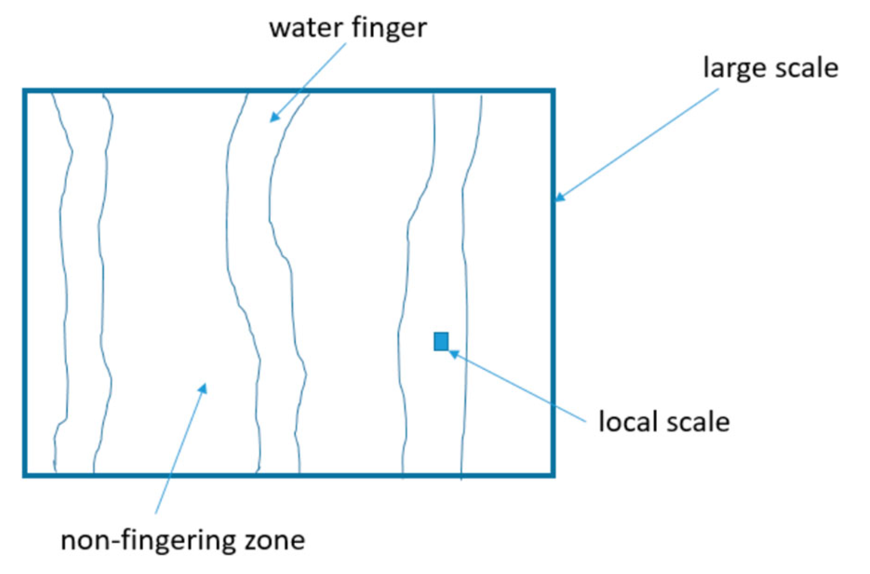
Figure 2.
The change of two flow fields per unit time in the REV of ARM.
Disclaimer/Publisher’s Note: The statements, opinions and data contained in all publications are solely those of the individual author(s) and contributor(s) and not of MDPI and/or the editor(s). MDPI and/or the editor(s) disclaim responsibility for any injury to people or property resulting from any ideas, methods, instructions or products referred to in the content. |
© 2026 by the authors. Licensee MDPI, Basel, Switzerland. This article is an open access article distributed under the terms and conditions of the Creative Commons Attribution (CC BY) license (http://creativecommons.org/licenses/by/4.0/).
Copyright: This open access article is published under a Creative Commons CC BY 4.0 license, which permit the free download, distribution, and reuse, provided that the author and preprint are cited in any reuse.


