
Submitted:
20 January 2026
Posted:
22 January 2026
You are already at the latest version
Abstract
Machine learning (ML) backtests in finance frequently overstate performance due to data leakage, non-point-in-time features, and evaluation procedures that inadvertently incorporate future information. This paper proposes a leakage-resistant, reproducible, and deployment-oriented framework, the Quant-Safe architecture, combining (i) point-in-time feature engineering with explicit reporting lags, (ii) walk-forward evaluation with out-of-sample (OOS) explainability, and (iii) a robust portfolio translation layer with transaction- cost modeling and execution-grade accounting logs. We validate the framework on the Dow Jones Industrial Average (DJI) constituent universe over 2015-2025, using gradient-boosted trees and Shapley Additive Explanations (SHAP) to demonstrate that macro regime variables (e.g., interest-rate proxies) become dominant drivers during stress periods. The primary contribution is an engineering methodology enabling other researchers to reproduce, extend, and audit financial ML results with explicit controls against common failure modes.
Keywords:
financial machine learning
; data leakage
; walk-forward validation
; explainable AI
; SHAP
; portfolio construction
; backtest overfitting
; execution logging
1. Introduction
The empirical finance literature increasingly applies ML models to return prediction and cross-sectional asset selection [1,2]. However, many reported gains fail to survive realistic deployment conditions due to data leakage, improper temporal splits, and missing trading frictions [3,4]. In parallel, explainable AI (XAI) techniques such as SHAP offer a path to interpretability and regime diagnostics, reducing “black-box” risk in investment decision-making [5,6,7].
This study adapts XAI-driven investment modeling to a stricter engineering standard. Rather than emphasizing headline returns, we emphasize auditability: point-in-time data semantics, leakage prevention, OOS explainability, and execution-consistent performance logging.
1.1. Contributions
We contribute:
- A Quant-Safe architecture defining operational safeguards for financial ML pipelines: reporting lags, point-in-time features, walk-forward evaluation, and OOS-only explainability.
- A formalized Algorithm 1 and a Data Leakage Failure Modes checklist aimed at reviewer scrutiny and reproducible research.
- A naïve vs Quant-Safe comparison table illustrating why common evaluation shortcuts inflate results.
- A reproducible implementation with execution-grade accounting logs (daily mark-to-market equity, realized/unrealized P&L by ticker, slippage proxies) and a Monte Carlo appendix for robustness.
2. Related Work
ML asset pricing and return forecasting have advanced rapidly [1,2]. Yet systematic over-optimism in backtests is well documented, including backtest overfitting [3] and leakage introduced by non-point-in-time features and improper cross-validation [4]. Interpretability frameworks such as SHAP [5] and general XAI guidance [6,7] motivate the use of explanation not merely as a diagnostic, but as a safeguard against spurious relationships.
On the portfolio side, we adopt robust, low-parameter constructions (top-N, inverse-volatility weights) consistent with the preference for simple, stable allocation rules under estimation error [8,9]. We also explicitly model transaction costs, which are central to realistic strategy evaluation [10,11].
3. Data and Experimental Design
3.1. Universe and Horizon
The research universe is the DJI constituent set used in the project codebase. The modeling target is a forward return proxy (as implemented in the pipeline), while the portfolio is rebalanced at a fixed schedule (monthly in the primary configuration).
Limitation (Survivorship Bias): If the study uses a modern constituent list retroactively, survivorship bias may inflate performance. The primary claim of this paper is the Quant-Safe methodology (leakage prevention + OOS explainability), not the absolute historical return magnitude. Future work should incorporate point-in-time constituent membership or investable proxies [4].
3.2. Macro and Risk Controls
We incorporate a minimal macro block designed to be easy to reproduce:
- Interest-rate proxy (e.g., 10Y yield series or yield-change z-scores)
- Risk/volatility proxy (e.g., VIX or realized volatility)
These variables enable regime attribution in SHAP and motivate risk scaling when volatility spikes.
4. Quant-Safe Methodology
4.1. Design Principles
The Quant-Safe architecture enforces:
- Point-in-time semantics: every feature must be available at prediction time.
- Reporting lags: fundamentals are shifted by a disclosure lag to avoid “trading on future filings”.
- Temporal evaluation: walk-forward or strictly OOS evaluation for research claims.
- Explainability discipline: SHAP computed on OOS folds only, preventing explanation leakage.
- Execution consistency: transaction costs, slippage proxies, and accounting-quality logs.
4.2. Algorithm 1: Quant-Safe Pipeline
| Algorithm 1 Quant-Safe Pipeline (Walk-Forward + OOS SHAP + Portfolio Layer) |
|
Require: Asset prices , macro variables , optional fundamentals with reporting lag Require: Prediction horizon H, rebalance schedule , cost model , top-N selection rule
|
4.3. Data Leakage Failure Modes (Reviewer Checklist)
Reviewers frequently reject financial ML work due to unaddressed leakage. Table 1 lists common failure modes and explicit mitigations.
4.4. Naïve ML Backtest vs Quant-Safe Evaluation
Table 2 clarifies why many “state-of-the-art” results do not survive deployment.
5. Modeling and Explainability
5.1. Model Choice
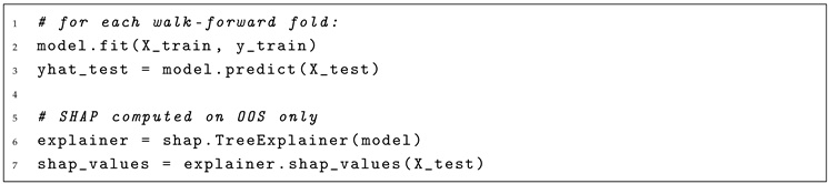
5.2. Out-of-Sample SHAP
SHAP decomposes predictions into additive feature attributions under a cooperative game-theoretic framework [5]. In this study, SHAP values are computed only on OOS test folds to preserve interpretability under real-time constraints and avoid explanatory leakage.
6. Portfolio Construction, Costs, and Accounting
6.1. Portfolio Translation Layer
We map predicted returns into an actionable portfolio:
- Selection: top-N assets by .
- Weights: inverse-volatility weights to reduce risk concentration [9].
- Rebalance: monthly (primary configuration).
- Turnover control: trade only when ranks change materially.
- Risk caps: max weight per name; optional regime-based gross reduction.
6.2. Trading Frictions
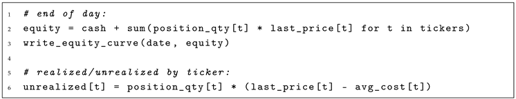
6.3. Accounting-Quality Logs
To ensure auditability, we persist:
- Daily mark-to-market equity curve
- Realized and unrealized P&L by ticker
- Trade blotter with fill reconciliation (broker fills matched back into records)
These records are required for credible research-to-production transfer.
7. Results (DJI Research Validation)
7.1. Performance Summary
7.2. Interpretation
A central claim is not “a magic alpha,” but that the explanation traces are economically coherent: rate-related and volatility-related features rise during tightening or stress regimes, consistent with discount-rate intuition and risk repricing.
8. Robustness Appendix: Monte Carlo via Block Bootstrap
Backtests are single-path realizations. We complement point estimates with Monte Carlo resampling of the realized strategy return series using a block bootstrap to preserve short-horizon dependence [13]. We report distributions of CAGR, volatility, and maximum drawdown.
Figure 3.
Monte Carlo equity fan chart (block bootstrap). Median path with percentile bands.
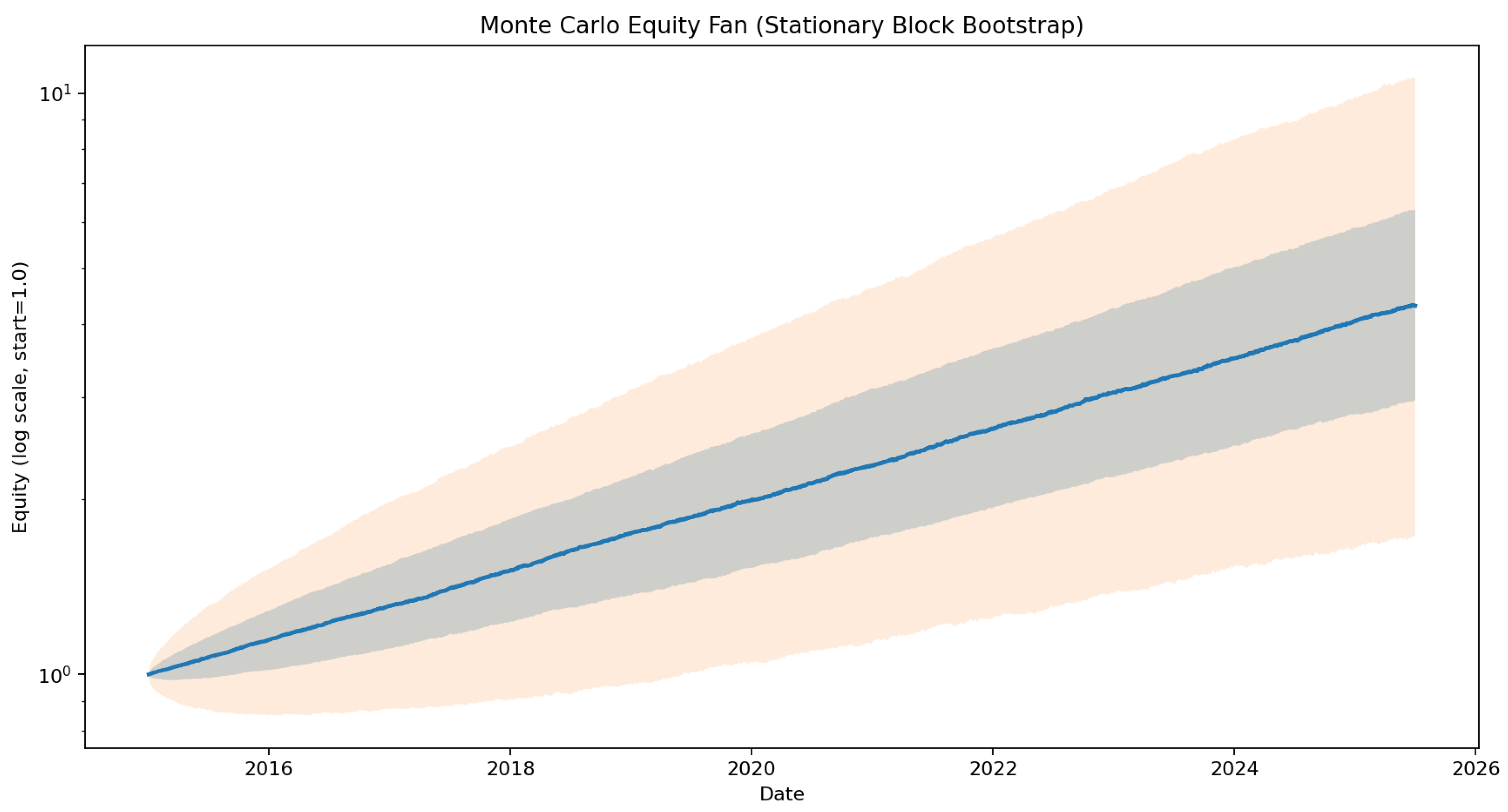
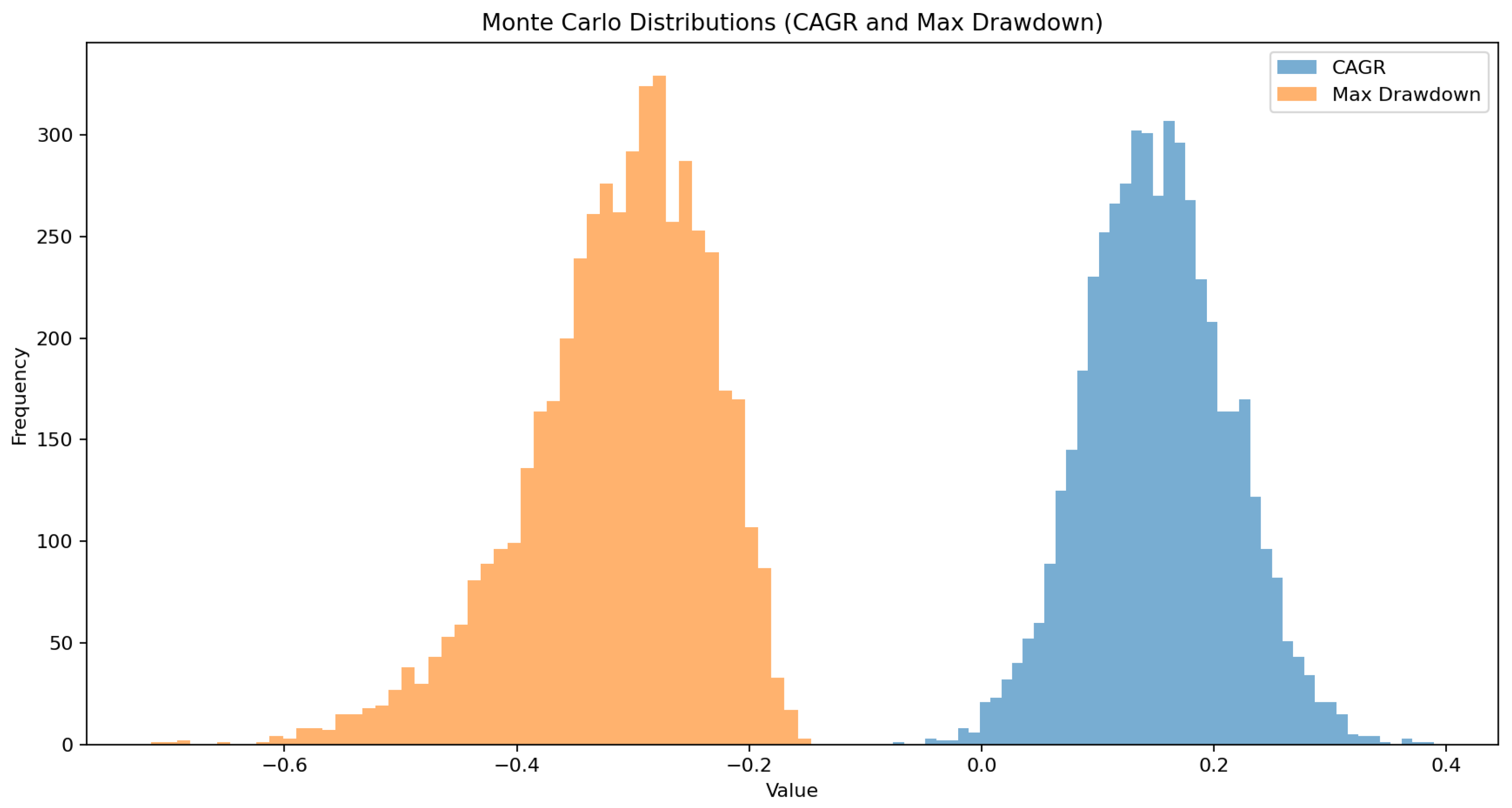
Figure 4.
Monte Carlo distribution summary (CAGR, max drawdown).
The code to generate these figures and LaTeX-ready tables is provided in the repository (see code/monte_carlo_appendix.py).

Table 3.
Monte Carlo block-bootstrap summary statistics for key performance metrics.
| metric | p05 | p25 | p50 | p75 | p95 | mean | std |
|---|---|---|---|---|---|---|---|
| CAGR | 0.054 | 0.109 | 0.150 | 0.192 | 0.253 | 0.152 | 0.061 |
| MaxDD | -0.462 | -0.359 | -0.303 | -0.256 | -0.204 | -0.314 | 0.080 |
| AnnVol | 0.180 | 0.191 | 0.202 | 0.214 | 0.234 | 0.204 | 0.017 |
| Sharpe | 0.356 | 0.608 | 0.786 | 0.980 | 1.264 | 0.797 | 0.276 |
9. Reproducibility: Minimal Code Excerpts
Short excerpts illustrate the reproducibility approach (full code in repository).
9.1. OOS SHAP Discipline (excerpt)
| Listing 1: OOS-only SHAP computation (conceptual excerpt) |
 |
9.2. Accounting Logs (excerpt)
| Listing 2: Execution-grade logs: MTM equity and per-ticker P&L (conceptual excerpt) |
 |
10. Limitations and Future Work
Key limitations include survivorship bias (if present), sensitivity to trading frictions, and the need for release-aware macro series. Future work will:
- incorporate point-in-time universe membership,
- expand regime switching (macro stress filters, volatility targeting),
- validate on additional universes (ETFs, ATHEX).
11. Data and Code Availability
Code and results are available on GitHub and archived on Zenodo:
- GitHub: KarmirisP/quant-safe-xai-portfolio
- Zenodo DOI: 10.5281/zenodo.18167108 [14]
Conflicts of Interest
The author declares no conflicts of interest.
References
- Gu, S.; Kelly, B.; Xiu, D. Empirical asset pricing via machine learning. Journal of Financial Economics 2019, 131, 335–360. [Google Scholar]
- Feng, G.; He, X.; Polson, N. Deep learning in characteristics-sorted factor models. Journal of Financial Economics 2020. [Google Scholar] [CrossRef]
- Bailey, D.H.; Borwein, J.M.; López de Prado, M.; Zhu, Q.J. The probability of backtest overfitting. Journal of Computational Finance 2017, 20. [Google Scholar] [CrossRef]
- López de Prado, M. Advances in Financial Machine Learning; Wiley, 2018. [Google Scholar]
- Lundberg, S.M.; Lee, S.I. A unified approach to interpreting model predictions. In Proceedings of the Advances in Neural Information Processing Systems, 2017. [Google Scholar]
- Molnar, C. Interpretable Machine Learning; Leanpub, 2020; Online book. [Google Scholar]
- Babaei, G.; Giudici, P. Explainable artificial intelligence (XAI) in investment decision-making. AI & Applications 2025. Preprint / working paper version archived in project materials. [Google Scholar]
- Markowitz, H. Portfolio selection. The Journal of Finance 1952, 7, 77–91. [Google Scholar] [PubMed]
- Clarke, R.; de Silva, H.; Thorley, S. Risk parity, maximum diversification, and minimum variance: An analytic perspective. Journal of Portfolio Management 2013, 39, 39–53. [Google Scholar] [CrossRef]
- Almgren, R.; Chriss, N. Optimal execution of portfolio transactions. Journal of Risk 2001, 3, 5–39. [Google Scholar] [CrossRef]
- Kissell, R. The Science of Algorithmic Trading and Portfolio Management; Academic Press, 2013. [Google Scholar]
- Chen, T.; Guestrin, C. XGBoost: A scalable tree boosting system. In Proceedings of the Proceedings of the 22nd ACM SIGKDD International Conference on Knowledge Discovery and Data Mining. ACM, 2016; pp. 785–794. [Google Scholar]
- Politis, D.N.; Romano, J.P. The stationary bootstrap. Journal of the American Statistical Association 1994, 89, 1303–1313. [Google Scholar] [CrossRef]
- Karmiris, P. Quant-Safe XAI Pipeline for Dynamic Portfolio Management (Code and Data Archive). Zenodo 2026. [Google Scholar] [CrossRef]
Figure 1.
Cumulative equity curve (strategy vs benchmark). Use log scale in plotting for interpretability of compounding.
Figure 1.
Cumulative equity curve (strategy vs benchmark). Use log scale in plotting for interpretability of compounding.
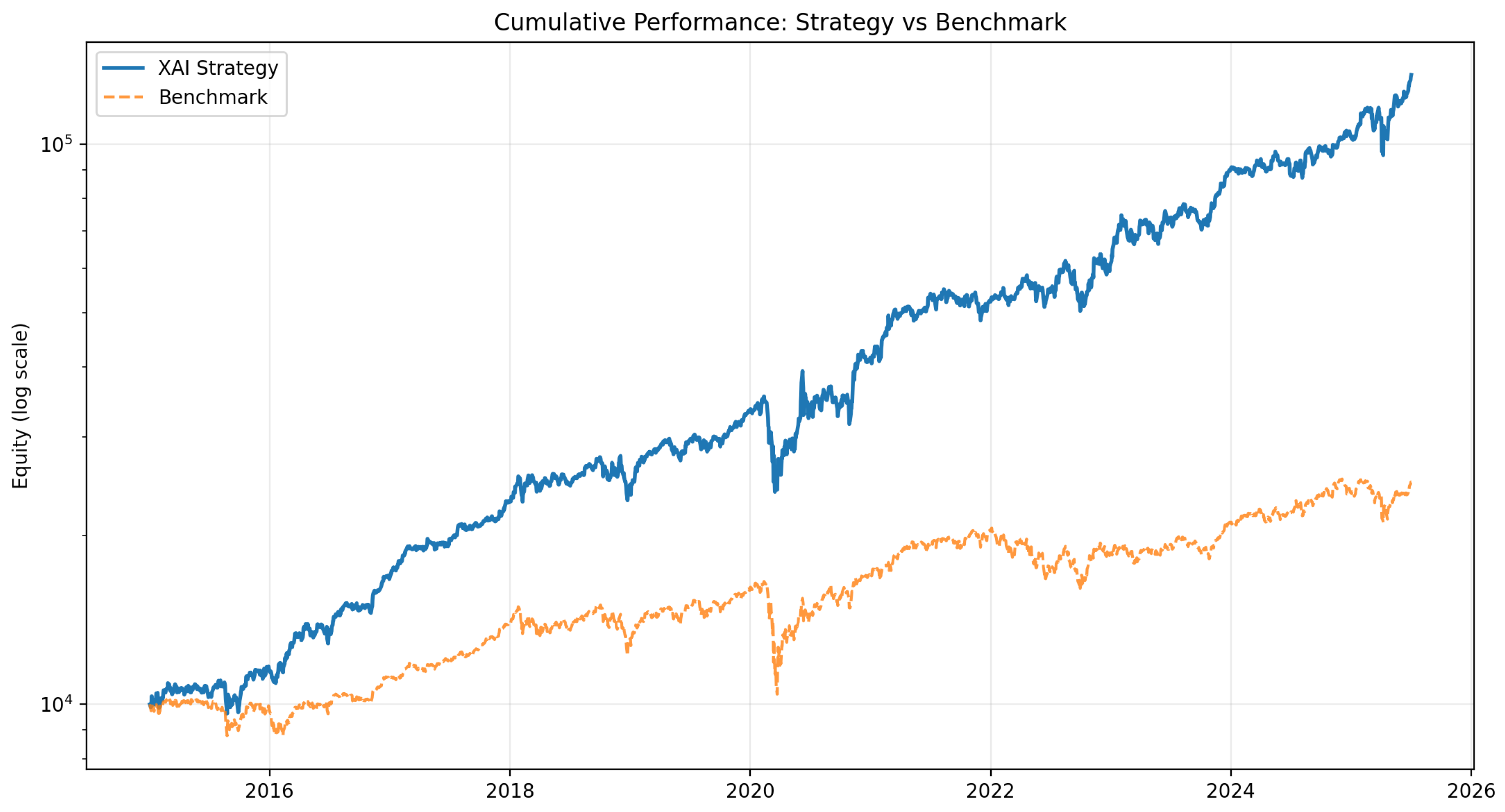
Figure 2.
Global SHAP importance (OOS). Macro / rate-regime variables increase in importance during stress periods.
Figure 2.
Global SHAP importance (OOS). Macro / rate-regime variables increase in importance during stress periods.
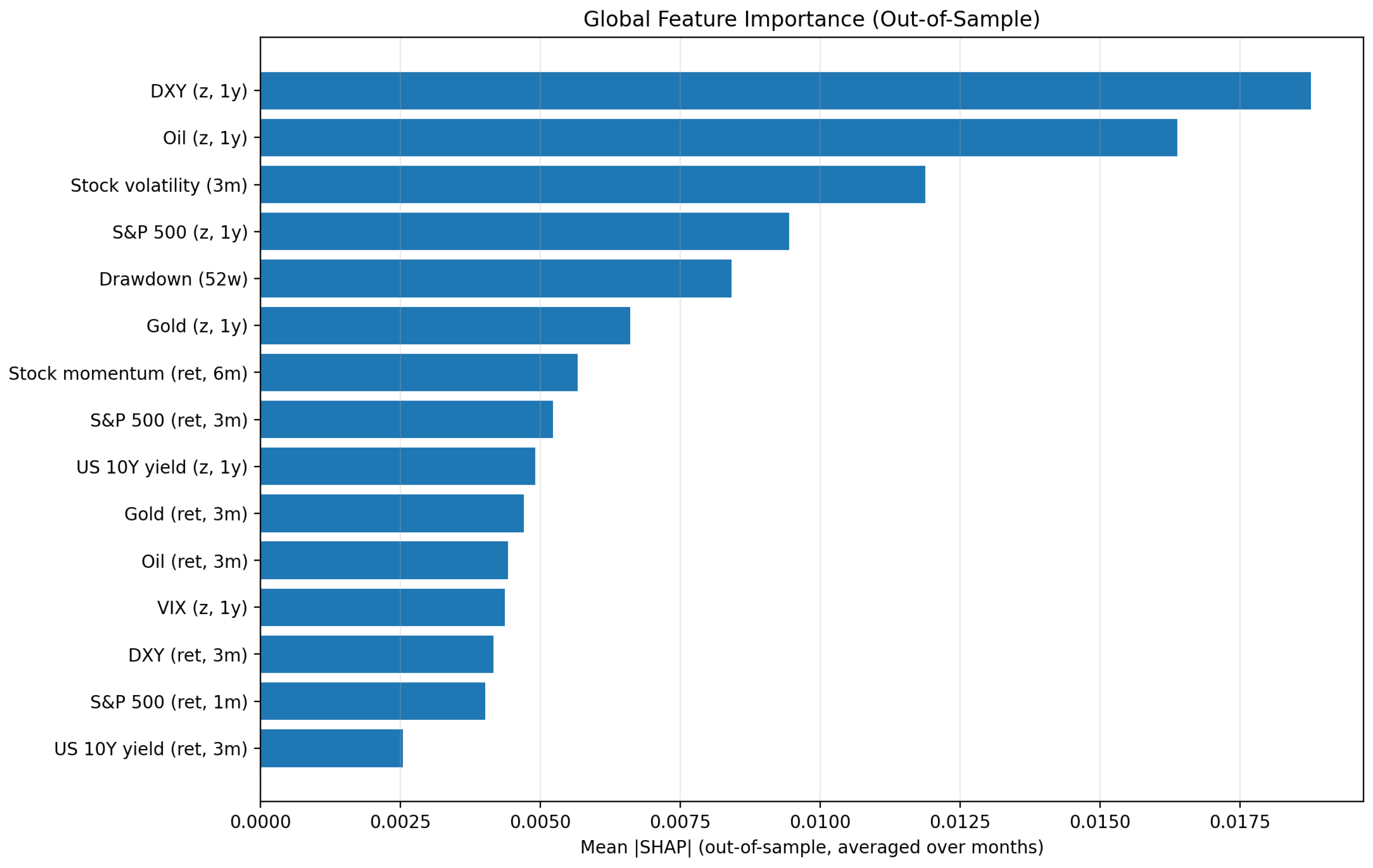
Table 1.
Common Data Leakage Failure Modes and Quant-Safe Mitigations.
| Failure Mode | How It Appears | Quant-Safe Mitigation |
|---|---|---|
| Look-ahead via random split | High CV scores; fails live | Walk-forward / time-ordered OOS only |
| Non-point-in-time fundamentals | “Predicts earnings surprises” unrealistically | Explicit reporting lag |
| Same-day macro availability | Using revised/late macro prints | Use release-aware series; conservative lag |
| Target leakage in features | Feature computed with data | Audit feature timestamps; unit tests |
| Survivorship bias in universe | Overstates long-run returns | Declare limitation; prefer point-in-time membership |
| Cost-free backtest | Unrealistically high turnover alpha | Cost model + slippage proxies |
| Explanation leakage | SHAP on train or post-fit full data | Compute SHAP only on OOS folds |
Table 2.
Comparison: Naïve ML Backtests vs Quant-Safe Architecture.
| Component | Naïve Implementation | Quant-Safe Implementation |
|---|---|---|
| Validation split | Random K-fold | Walk-forward (expanding/rolling) |
| Fundamentals | Use as-of values without lag | Lag by disclosure delay |
| Feature scaling | Global z-score | Cross-sectional or time-safe scaling |
| Explainability | SHAP on full dataset | SHAP strictly OOS per fold |
| Portfolio layer | Optimized weights, unconstrained | Top-N, inverse-vol, caps, turnover control |
| Trading frictions | Often omitted | Explicit costs + slippage proxies |
| Accounting | P&L only | MTM equity + realized/unrealized by ticker + reconciliation |
Disclaimer/Publisher’s Note: The statements, opinions and data contained in all publications are solely those of the individual author(s) and contributor(s) and not of MDPI and/or the editor(s). MDPI and/or the editor(s) disclaim responsibility for any injury to people or property resulting from any ideas, methods, instructions or products referred to in the content. |
© 2026 by the authors. Licensee MDPI, Basel, Switzerland. This article is an open access article distributed under the terms and conditions of the Creative Commons Attribution (CC BY) license (http://creativecommons.org/licenses/by/4.0/).
Copyright: This open access article is published under a Creative Commons CC BY 4.0 license, which permit the free download, distribution, and reuse, provided that the author and preprint are cited in any reuse.


