
Submitted:
19 January 2026
Posted:
21 January 2026
You are already at the latest version
Abstract
Leakage detection in water distribution networks is critical for effective localization to address water scarcity, yet the scarcity of correctly annotated leak events limits the use of supervised learning methods. Generating hydraulic simulation-based datasets are often challenging due to incomplete network topology and sparse sensor coverage. Unsupervised approaches relying on single-model-anomaly scores frequently struggle to balance sensitivity and accuracy. This study proposes a regression-ensemble framework that learns the District Metered Area (DMA)-specific demand-supply dynamics to detect emerging leaks using smart meter data. Regression models - Random Forest, Support Vector Regression, XGBoost, and Multi-Layer Perceptron, are trained on DMA-consumption and supply data – preprocessed to preserve background leakage while detecting and correcting emerging leaks. Deviations between predicted and observed supply are quantified through Pearson correlation, Kendall’s Tau, and Z-score, whose anomaly indications are combined at metric and model levels using weights derived from model-prediction accuracy. A leak is identified once the ensemble anomaly-score crosses a threshold. The system reliably detects leaks within 8-12 hours of onset, achieving 91\% accuracy on simulated leak scenarios and 98\% accuracy for available real leak cases with 0.5 as the anomaly-score threshold. Our proposed framework demonstrates the potential of smart meter-driven ensemble analytics for rapid and robust leak detection.
Keywords:
leakdetection
; real-time
; unsupervised learning
; regression modeling
; artificial intelligence
; ensemble learning
; machine learning
; water distribution networks
; smart meter data
; district metered area
1. Introduction
In the face of growing water scarcity across the globe, effective management of non-revenue water (NRW) loss [1] is a challenging task in day-to-day operations of water distribution networks (WDN). WDNs are complex systems that are responsible for managing water demand among the consumers with promised water quality by transporting treated water through extensive pipe networks to end-consumers. However, these networks are susceptible to failures caused by factors such as corrosion, pressure fluctuations, defective materials, and environmental stressors like soil erosion and extreme weather conditions [2]. These vulnerabilities frequently lead to leaks in water distribution networks (WDNs), resulting in significant water losses. Globally, an estimated 30% of treated water is lost by utilities before it reaches end-consumers [3]. As per the International Water Association (IWA) definition, NRW loss encompasses both physical losses due to leaks and commercial losses, such as metering inaccuracies and unauthorized consumption [1]. These inefficiencies represent an annual economic burden of approximately $39 billion worldwide [4]. Beyond financial impacts, leakage increases energy consumption, as additional pumping is often required to maintain adequate system pressure and performance, leading to increased carbon footprint [5]. Undetected leaks pose serious risks to public safety and environmental balance by contributing to sinkhole formation, land subsidence, and pipe bursts [6].
The advancement of Automated Metering Infrastructure (AMI), together with the widespread adoption of DMAs in WDNs, has enabled the measurement of NRW loss at finer spatial resolution than at the overall network level [7,8]. Accurate leakage detection at the DMA-level not only increases the reliability of subsequent of leak-localization-frameworks, but also substantially reduces the search space spatially for localization, thereby lowering the computational burden on subsequent localization processes [9]. However, in reality, each DMA typically exhibits pre-existing background leakage [10]. Additionally, variations in AMI coverage and quality across DMAs contribute to differing levels of apparent losses [1,11]. As a result, early detection of leaks of varying magnitudes and distinguishing newly emerging physical losses from existing background NRW-loss, remains challenging for utilities, particularly in the absence of expert systems [12] and diminishing expert-knowledge due to retiring workforce [13]. Moreover, developing a modular and scalable data-driven framework that can accommodate heterogeneous WDN conditions while reliably detecting leak onsets within operationally meaningful time-frame remains a significant research and implementation challenge [14]. Static thresholding of NRW loss methods fail to capture anomalies, while facing the dynamic evolving behavior of WDN [15], and a significant share of detected anomalies—typically are not actual leaks but rather operational variations or sensor drift [16].
2. Related Works
Over the past decades, significant advances have been made in leak detection and localization technologies for WDNs. However, the reliability of leak localization remains highly dependent on the accuracy of leak detection. An effective leak detection system thus serves as a critical prerequisite for precise leak localization [17]. Moreover, near real-time detection enables early activation of localization methods, facilitating timely intervention and contributing directly to the reduction of NRW-losses [18].
Advancement of Data Science (DS) and Machine Learning (ML) over the past years has contributed to emerging data-driven technologies for Leakage detection in WDNs. Sousa et. al. [19] demonstrated application of supervised and unsupervised ML techniques to classify leak and no-leak events from a leak-labeled dataset of pump-pressures in a DMA of a Swedish WDN. In reality, due to operational resoure-limitation, having such an extent of leakage-annotation is a viability-concern, considering the extensive variety of digital maturity standard of WDNs. Britto et. al. [20] proposed Random Forest (RF), Naive Bayes (NB), and Decision Tree (DT) driven supervised leak detection using flow-induced acoustic signals in a lab-scale pipeline. However, the work does not contain sufficient evidence of performance in uncontrolled real-world environment containing demand variations, pipe corrosions and background leaks. Ravichandran et al. [21] proposed a Multi-Strategy Ensemble Learning (MEL) framework for acoustic-based leak detection, formulating the task as binary classification using representations like power spectral density and time-series data. By combining multiple Gradient Boosting Tree classifiers through bagging, the approach achieved 99.84% accuracy with perfect sensitivity and 99.84% specificity, drastically reducing false positives from 238 to 23. This ensemble method demonstrated strong robustness and operational reliability for practical utility deployment. However, the efficacy of such system is highly reliant on the availability of acoustic sensors densely spread across the WDN.
Majority of supervised and semi-supervised leak detection frameworks require hydralic-simulation-driven dataset generation. Mashhadi et. al. [22] used EPANET to generate leak-scenario datasets comprising of leak-effects on nodal pressures, and employed several ML supervised (such as logistic regression, decision tree and random forest, artificial neural networks) classification and unsupervised (such as K-means, PCA) clustering methods to detect zonal-level leakages. Yu et al. [23] proposed a data-driven leak detection method that combines Kriging interpolation with a VGG16 Convolution Neural Network (CNN) to transform pressure data into spatial images for anomaly-based classification, achieving a 98% true positive rate and outperforming traditional models. However, its reliance on a dense sensor network, fixed detection threshold, and validation on a small-scale system limit its scalability to larger, more complex networks. Basnet et al. [24] have leveraged an ML framework for leak detection in WDS by combining EPANET-based hydraulic modeling with supervised learning. Their approach trains Multilayer Perceptrons (MLPs) and 1-D CNNs on simulated pressure differences from leak-free and leak scenarios, evaluating model performance under four noise conditions: no-noise, demand-noise, mixed-noise, and random leaks.
Fan et al. [25] propose a Clustering-then-Localization semi-supervised framework for leakage detection and localization in water distribution networks. First, the network is partitioned into hydraulically meaningful virtual zones using a modified K-Means algorithm that incorporates a hydraulic-distance metric and enforces graph connectivity. For each zone, pressure and flow monitoring data under normal and leak conditions are used to construct feature representations. A reconstruction-based Autoencoder (AE) and Principal Component Analysis (PCA) model is then trained to detect leakage events and to identify the most likely affected zone, even when only limited labeled leak data are available. Rajabi et al. [26] introduced a semi-supervised leak detection method in which synthetic leak and non-leak scenarios are generated using hydraulic simulations on the benchmark L-Town network. The resulting pressure and demand time-series data are spatially interpolated via Kriging to produce image-based representations of network states. A conditional deep convolutional generative adversarial network (CDCGAN) is then trained to classify these representations, enabling leak detection with limited labeled data.
Although used as a suitable benchmark, these methods are based on idealized hydraulic simulation which ignores the real-world elements like background stationary leakages, demand variability and pipe deterioration [17,27,28]. Detection of leakages based on hydraulic simulation in a real-world scenario requires topology-specific optimal placement of quality pressure-sensors with sufficient quantity [29]. Hydraulic simulation-based methods require extensive computational simulation to create leak-scenario-aware dataset for classification to cover variety of hydraulic conditions [30]. Most importantly, hydraulic simulation of physical water networks is often hindered by the difficulty of generating a fully connected graph representation of the WDN. This challenge largely stems from the substantial automated and manual preprocessing required to achieve network connectivity, which is necessitated by the wide variability in digital maturity among utilities and the lack of standardized GIS data formats within the water sector [30,31].
In a nutshell, supervised and semi-supervised learning techniques, specially deep neural networks demonstrate strong leak detection accuracy and robustness. However, they face common challenges such as the scarcity and difficulty of obtaining large, accurately labeled datasets, due to the infrequent and varied nature of leaks [17]. Therefore, they lack the validation of leak events in real world complexities of WDNs. Since these models rely heavily on specific sensor configurations, their applicability across various WDS topologies remains limited.
Unsupervised leak detection technologies acts as a viable substitute in real world utility industries for detecting leakages without needing extensive labeled dataset. Yu et al. [32] introduced an unsupervised GPR-based framework for pipeline leak detection, extracting velocity and energy features from B-scan profiles and clustering them using DBSCAN to distinguish leak-affected areas without labeled data, achieving 92% accuracy. While effective and adaptable across materials, it requires manual DBSCAN tuning, prior knowledge of pipeline geometry, and is sensitive to subsurface variations that may cause misclassification. Leonzio et al. [33] employed a convolutional autoencoder trained on no-leak pressure data to detect anomalies, achieving 89-94% accuracy and 13-hour detection delay on the LeakDB dataset, which is substantially faster than Minimum Night Flow methods. However, its high computational cost, reliance on synthetic data, and threshold sensitivity under varying demand limit real-world scalability. Quiñones-Grueiro et al. [34] combined PCA with periodic transformations and dynamic augmentation to detect leaks via multivariate statistics (T-square, SPE, and RBC indices), achieving 85% accuracy on the Hanoi WDN. Yet, performance degraded near zone boundaries, sensor faults were often misclassified as leaks, and trade-offs between sensitivity and accuracy persisted. Furthermore, unsupervised anomaly detection methods that rely on a single machine learning model and a single anomaly score often struggle to balance timeliness and reliability, leading to increased false alarms or delayed leak detections [17,35]. In addition, the detection capability reduces if the training data are not represented by the minor leakage pattern or normal pattern sufficiently [36]. Furthermore, the baseline “normal” operating conditions of a water network evolve once a leak begins to develop. Consequently, detecting emerging leaks must be performed with respect to this updated normal state [37]. Therefore, we need adaptive models that understand context and status-quo situation of the WDN.
Emergence of AMI technology has enabled utilities with automated billing processes. However, the same data are used for water balancing purposes at DMA-level. Measurements of water delivered to a DMA and water consumed, easily showcase the variation of NRW loss within a period [38]. With advanced radio networks, frequent consumption and delivery measurements can be obtained that enable timely detection of leakages. Glomb et al. [37] demonstrated that leak detection in water networks can be achieved using a range of unsupervised machine-learning and deep-learning methods, including k-Nearest Neighbours, Local Outlier Factor, Isolation Forest, One-Class SVM (Support Vector Machine), PCA, AE, ECOD (Empirical cumulative distribution functions) and COPOD (Copula-based outlier detection). Their features comprised DMA-level consumption, supply, pressure, and estimated losses. The study showed that their approach was capable of identifying leaks within 24 hours of their onset. However, the work did not provide a detailed quantitative evaluation of leak-detection performance using standard classification metrics, nor did it assess the scalability of the framework across multiple DMAs. Moreover, as noted earlier, the requirement for pressure-sensor data in every physically established DMA represents a significant practical limitation for many utilities. Nevertheless, their framework serves as an important inspiration for our proposed method, which aims to achieve similar capabilities with a substantially reduced data burden.
3. Contributions of This Work
Our work leverages AMI data, DMA adoption and contributes a novel approach to leak detection in WDNs, which overcomes important constraints of the existing methods, regarding robustness, result-interpretation, viability and the necessity of labeled training-data. Following are the research contributions of our proposed framework:
- Novel DMA-level leak detection framework based on causal demand-supply dynamics modeling: We introduce the first framework that learns the causal relationship between DMA-level supply and consumption to detect leaks by statistically comparing predicted and observed supply. This represents a new paradigm for early leak detection in water distribution networks.
- Robust, scalable and modular ensemble ML pipeline for early leak detection: Our method provides a modular and maintainable unsupervised ensemble pipeline-combining RF, SVR, MLP, and XGBoost—that reliably detects leaks within 8-12 hours of onset. The pipeline detects emerging new leaks while retaining background leakages with an automated calibration mechanism.
- Advanced statistical fusion of multi metric leak indicators for leak-detection: We introduce a dynamic leak-indicator derivation strategy using multiple statistical scores (Pearson correlation, z-score, Kendall’s tau) together with a novel weighted ensemble fusion mechanism, improving robustness and reducing false positives across real-world DMAs.
4. Materials and Methods
4.1. Core Principle of Proposed Framework
The core-principle of our proposed framework stands on understanding DMA-wise relationship between consumption and supply. The preprocessed data from all consumer meters in a specific DMA are aggregated to calculate DMA-wise consumption at time t, as illustrated in Section 4.3.1. DMA-wise supply at time t is calculated by using the preprocessed inlet and outlet meter measurements (refer to Section 4.3.1).
The time-series representation of water consumption and supply for a period of 7 days are shown in Figure 1, exhibit a causal and correlative relationship in an non-anomalous scenario. In a pressurized WDN, any increase or decrease in consumption within a DMA alters the local hydraulic balance, causing a corresponding rise or fall in inflow through the district meter that supplies the area. Such relationship is broadly exhibited in presence of minor or background leakages. The magnitude difference between supply and consumption is caused broadly due to the NRW loss within a DMA. The difference between delivery and consumption normalized by delivery provides NRW loss%. Due to new emerging leakages, rise in NRW loss% is observed for the compensatory changes in hydraulic pressure. This leads to proportional adjustments in the inflow measured at the supply time-series, given that there is no increase in apparent loss (refer to Figure 8). Hence, , the supply at time t, can be modeled in the form of consumption, and NRW-loss, as follows:
Due to emerging leakages in a DMA, non-linearity is introduced between supply and consumption. Even when there is no new emerging leak, due to variable amount of background leaks and variable amount of apparent-loss across different DMAs, non-linearity is introduced in the supply-consumption relationship [37].
Therefore, our methodology is built on the core principle (Figure 2) of exploiting and learning the existing consumption–to–supply relationship across several DMAs. In the proposed framework, each regression model learns to predict a supply window of length ℓ for DMA d using the corresponding consumption window.
For a given DMA d and window index i, the input consumption window is defined as
and the model is trained to estimate the corresponding supply window
This training is performed using preprocessed supply data in which newly emerging leaks are identified and rectified, while DMA-specific background NRW losses may still be present (details in Section 4.3.2). During inference, the predicted supply window is compared with the observed supply window,
using multiple statistical metrics. Significant deviations between and indicate a disruption from the DMA’s steady-state behavior and may correspond to a leakage.
The outputs of these statistical metrics are combined to form an anomaly score, and an anomaly is flagged when this score exceeds a decision threshold () from a predefined set of candidate values (refer to Section 4.4.3). The subsequent sections describe the method overview and each component of the proposed DMA-level leak detection framework in detail.
4.2. Method Overview
Figure 3 illustrates the end-to-end high-level system workflow of our proposed framework which consists of two working stages – Offline Consumption-Supply modeling and Online Leak Detection.
In Offline Consumption-Supply modeling stage, multiple ML regression models are trained and evaluated on the consumption and leak-corrected supply data. In the Regression Model Training sub-stage, first, the hourly consumption and supply are computed for each DMA d using preprocessed smart meter measurements from end-consumer meters, district meters and meter-to-DMA mapping (refer to Section 4.3.1). Since the approach is unsupervised, regression models are expected to learn the non-anomalous behavior of the data. To facilitate this, an automated mechanism of offline leak-identification and correction (refer to Section 4.3.2) using time series segmentation is integrated to detect and correct potential leak indicators, while invalid values (e.g., supply values lesser than consumption) are filtered out and corrected. This automation essentially acts as a calibration step, eliminates the necessity of manual leak-period labeling and simplifies the integration of new utilities into the system while guaranteeing that training data represents calibrated conditions.
Next, the Feature Extraction (refer to Section 4.3.3) step constitutes of scaling and formatting the input data for models, for effective training. a Min-Max scaler is applied within each DMA to ensure consistency across regions. The supply and consumption time-series data are parsed and segmented using a 24-hour sliding window during feature extraction to record daily consumption-supply behavior. Furthermore, DMA names are one-hot-encoded to incorporate DMA-specific information. These processed inputs enable effective learning of DMA-wise relationships, and the Regression Model Training is performed using the resulting features and target supply data.
During the Regression Model Evaluation, Regression Model Opinion (RMO)-weights are derived from the accuracy calculated using the mean absolute percentage error (MAPE) between each regression model’s estimated and ground truth supply across the test set (refer to equation 18). These weights are then combined at both the model- and DMA-levels, ensuring that models with lower errors have greater influence in the leak detection process. Moreover, each model’s performance can vary across DMAs due to variability in data quality and model-specific strengths and limitations. Simultaneously, statistical distribution modeling is performed to establish Metric-Model-DMA (MMD)-thresholds. The thresholds are determined by computing statistical metrics such as Kendall’s Tau, Z-score, and Pearson correlation between each model’s estimated supply and the corresponding observed supply, extracted from the same test-set. These metrics are then aggregated for each model-DMA combination. All trained models and essential artifacts, including thresholds, weights, scalers, and encoders, are stored in a centralized repository to ensure reproducibility and facilitate Online Leak Detection.
In Online Leak Detection stage, features and observed supply are extracted from incoming DMA-specific supply and consumption data. DMA-specific supply and consumption are calculated using preprocessed meter data (refer to Section 4.3.1). The extracted features are subjected to the trained regression models to generate the predicted supply. Note that the leak-correction step is not exhibited in this stage. Trained models and their associated artifacts are loaded from the centralized repository, and each model produces an estimated supply based on the given consumption data.
Statistical metrics are then computed by evaluating the deviation between each model’s estimated supply and the observed supply. The resulting metric scores are compared against the predefined MMD-thresholds from the training phase. First, in a Metric-level ensembling each regression model-generated prediction and observed supply is compared using multiple statistical metrics to determine a consensus on the presence or absence of a leak. Next, these metric-level consensus outputs from all regression models are combined in a Model-level ensembling, where each model contributes according to its RMO-weight. The outcome of this two-stage fusion process is a unified anomaly score ranging from 0 to 1, representing the likelihood of a leakage.
To evaluate performance, the anomaly score threshold (operating point ), beyond which a leakage is indicated, is systematically varied. This enables the assessment of the method’s detection capability under different decision boundaries. The resulting classifications are then compared against labeled leak events, and the accuracy of the proposed approach is quantified using standard classification metrics such as precision, recall, F1-score, and Area Under Curve (AUC).
4.3. Offline Consumption-Supply Modeling
4.3.1. DMA Supply and Consumption Calculation
Before preparing DMA-level supply and consumption, meter level preprocessing is performed. Each meter reports a cumulative volume index from which water consumption is obtained by differencing successive readings. Consumer meters provide household-level usage, while district meters record hourly inflow and outflow at the DMA level. Both data types undergo identical preprocessing to ensure consistent flow computation:
- Monotonicity check: Cumulative readings should never decrease but drops are typically caused by resets or transmission errors, which is corrected by replacing the value with the previous valid reading.
- Linear interpolation: Missing or irregularly sampled readings are filled using linear interpolation, assuming gradual changes in consumption.
- Flow calculation: First-order differencing on cleaned cumulative values yield instantaneous flow, producing a time-resolved flow data for downstream analysis.
Once individual meter-level consumption is calculated and validated, the hourly consumption at the DMA level is obtained by summing the readings of all consumer meters within that DMA. The total consumption at time t for DMA d, denoted as , is given by:
where represents the hourly preprocessed consumption recorded by the k-th consumer meter. This combined consumption serves as an input for estimating the water supply.
The DMA-level supply is calculated using the hourly-resolution flow of inlet and outlet meters. This is done by aggregating the flow of inlet meters and outlet meters separately, and then calculating the difference between these aggregated values to obtain the supply. For each DMA at time t, the total flow of inlet meters, denoted as , is computed as:
Similarly, the aggregated flow of outlet meters, , is given by:
The net water supply for the DMA, denoted as , is computed as the difference between the total inlet and outlet flow:
In a DMA, if there are no outlet meters, the outlet volume is taken as zero so that there is no overestimation of the supply. Figure 4 illustrates the consumption and supply for two representative DMAs.
4.3.2. Preprocessing and Leak-Correction
The consumption-supply relationship at the DMA level often exhibits inconsistencies due to outliers, sensor faults, and NRW losses. Among these, leaks constitute a major source of NRW loss, occurring when the recorded supply exceeds the total measured consumption significantly, indicating water loss within the DMA before reaching consumers.
To ensure reliable regression model learning of consumption-supply relations, the data must be systematically corrected for both outliers and leakage. The correction procedure is described as follows:
-
Outlier Detection: Before analyzing leak patterns, it is necessary to correct unreasonable or missing loss values that may arise from meter faults or data transmission errors. The NRW-loss fraction at time t for DMA d is defined as:where , , and denote the loss fraction, supply, and consumption, respectively.Negative or greater-than-one loss values are considered invalid, as are extreme outliers that deviate by more than three standard deviations from the mean. To ensure statistical robustness, the median loss for each DMA—computed using only valid values within the range [0, 1]—is used to replace all invalid or missing loss entries:
-
Offline Leakage Segmentation: This step potentially acts as a calibration process to ensure robust learning of steady-state relations between DMA-wise supply and consumption. Note that this step is applied only to Regression Model Training process. After outlier correction, potential leakage patterns are identified by analyzing the temporal behavior of the corrected loss values. Rolling statistics are computed over a 24-hour window to capture daily variations:These features result into , which are clustered using K-Means into two categories representing normal and leak conditions:The clustering quality is evaluated using the silhouette score, and results with a score above 0.7 are considered valid for correction. Loss values belonging to the leak cluster are replaced with the median loss :
- Supply Correction: Finally, the corrected loss values are used to recalculate the corresponding supply values, ensuring internal consistency between consumption and supply. The refined supply for each DMA is obtained as:where and represent the refined supply and corrected loss at time t, respectively. This final correction ensures that the dataset accurately reflects realistic supply conditions for subsequent modeling of non-anomalous consumption-supply relationship. Figure 5 shows the supply data before and after removing invalid data, whereas Figure 6 illustrates the effect of leak data correction.
4.3.3. Feature Extraction
At this stage, preprocessed time-series data are transformed into a format suitable for regression model training. The procedure consists of normalization, temporal windowing, and categorical encoding to enable unified learning of DMA-specific consumption–supply relationships within a single model ensemble.
Since water consumption and supply magnitudes vary significantly across DMAs due to differences in population and infrastructure, Min-Max normalization is applied independently per DMA to scale both consumption and supply into the range . This normalization emphasizes pattern-based relationships while mitigating magnitude-induced bias toward high-consumption DMAs, resulting in scaled consumption and scaled supply .
Following normalization, overlapping input–output samples are generated using a rolling window of fixed length 24 hours and a step size of one hour. For a given DMA d, the i-th input and target samples are defined as:
where to denote consecutive hourly time steps. This sliding-window formulation preserves temporal input-output relationship, while increasing the effective number of training samples.
To incorporate DMA-specific information without constructing separate models, DMA identifiers are encoded using one-hot vectors. Let denote the encoding for DMA d among n total DMAs:
The final input vector for sample i is formed by concatenating the scaled consumption window and the DMA encoding:
which enables the regression models to jointly learn temporal consumption dynamics and DMA-specific characteristics.
4.3.4. Regression Model Training
The DMA-level consumption–supply relationship is learned using four regression models – MLP, SVR, RF, and XGBoost, to produce accurate supply estimates from consumption data. These models are selected for their explainability and because they span four distinct algorithmic paradigms: neural networks, support-vector methods, decision trees, and gradient boosting.
The overlapping samples obtained from feature engineering are used to train the regression models, where the training set is represented as,
Each regression model learns a hypothesis
where denotes model parameters and is the predicted supply vector. Each model is trained to minimize the Mean Squared Error (MSE) between the predicted and actual supply sequences:
4.3.5. Regression Model Evaluation
After training, each model generates predictions on unseen test samples,
where represents the scaled consumption vector and DMA encoding, and denotes the scaled target supply vector.
To restore original units of predicted supply, inverse scaling is applied as follows:
where denotes the inverse-scaled predicted supply vectors, and denotes the maximum and minimum scaler values used during min-max normalization of . This inverse scaling restores the physical meaning of all variables, enabling consistent evaluation and interpretation of model predictions for leak detection and performance assessment. This evaluation stage leads to calculation of Ensemble Artifacts using the estimation of following parameters:
-
RMO-weights estimation: To ensure the influence of models with superior predictive performance in leak-detection step, Regression Model Opinion (RMO) weights are computed as functions of their mean prediction accuracy across all test samples. We first evaluate the regression model performance using MAPE in fractions for model m in DMA d for individual test sample j as,Therefore, the average accuracy, representing the RMO weight for model m in DMA d, is computed using the mean of prediction accuracy across all test samples as follows:where is the number of test samples in DMA d. Since , the resulting RMO weights are guaranteed to satisfy .
-
MMD thresholds Estimation: Statistical Metric-Model-DMA (MMD) thresholds are computed for each DMA–model pair, using all test samples used in the Regression Model Evaluation. Given the observed and predicted (inverse-scaled) supply sequences and for DMA d, model m, and test sample j, the statistical metrics are defined as:where and denote Pearson and Kendall-Tau correlation coefficients, respectively, and represents the mean z-score across the 24-hour window of length . Distance-based metrics are avoided, as gradual changes in background NRW loss can bias magnitude-based deviations. Instead, pattern-based correlations and standardized differences are used to capture structural anomalies.Since the distributions of Pearson and Kendall-Tau correlations are sensitive to skewness due to high correlation between supply and consumption in no-emerging-leak scenario, their scores are normalized via a quantile transformation:where maps the empirical distribution to a Gaussian-like space, preserving rank order and improving robustness to outliers. The Z-score values remain unchanged, as they are inherently standardized.For each DMA–model pair, the transformed metric distributions across all test samples J are summarized by their mean and standard deviation:where and denotes the quantile-transformed version (for correlation metrics only).The leak detection MMD thresholds are then derived as:These thresholds define acceptable deviation ranges between observed and estimated supply, establishing a robust leak detection across all DMA-model combinations.
4.4. Online Leak Detection
In Online Leak Detection stage, DMA-level consumption and supply are aggregated using preprocessed smart meter data and the same calculation logic mentioned in Section 4.3.1. Then feature vector and target (observed supply) are extracted following the same principle mentioned in Section 4.3.3.
4.4.1. Statistical Comparison
The trained regression models consuming the extracted feature vector generate the predicted supply. Next, statistical metrics—Pearson correlation (), Kendall’s Tau (), and z-score (Z)—are computed for each DMA d, model m, and sample s by comparing the observed supply with the predicted supply of sample. An anomaly is flagged when a metric violates its model- and DMA-specific threshold:
Here, denotes the anomaly flag for metric , with respective thresholds , , and .
4.4.2. Anomaly Score Module
Anomaly score estimation consists of a two stage ensembling process:
-
Metric-Level Ensembling: To derive a single anomaly decision per model, the metric indicators are combined using two approaches:
- 1.
- Majority Voting (MV):
- 2.
-
Proportional Scoring (PS):where is the number of metrics, and provides a continuous anomaly score.
-
Model-Level Ensembling: Once metric-level results are obtained, model-level aggregation combines all model outputs within a DMA using RMO weights using the following approaches:The final scores and represent the ensemble leak-likelihood score for sample s in DMA d, integrating both metric- and model-level decisions weighted by model reliability. Our experiments are conducted using both the metric- and model-level ensemble approaches for a comprehensive evaluation.
Since all metric-level anomaly indicators are either binary or normalized to lie in , and the model-level ensembling is performed using a convex weighted average with non-negative RMO weights , the resulting ensemble anomaly score is guaranteed to be bounded within the interval . Given the fact that , the normalization ensures a valid probabilistic interpretation of the anomaly score.
4.4.3. Leak Detection
The anomaly decision threshold is selected from a predefined set of candidate values , where . The optimal threshold is determined as
where denotes the detection performance metric (refer to Section 4.5). Hence the predicted leak or no-leak label is obtained using,
where indicates whether the anomaly score is derived from Majority Voting (MV) or Proportional Scoring (PS), indicates predicted label, and denotes the indicator function, which returns 1 if , else 0 is returned.
4.5. Evaluation Criteria
As shown in Section 4.3.5, MAPE (refer to equation 17) inherently acts as a performance evaluation criteria for the consumption-to-supply prediction module. Furthermore, root-mean-squared-error (RMSE) is used to evaluate the regression models. RMSE for test sample j in DMA d using the prediction of model m is expressed as:
The overall system is evaluated in terms of efficacy in leak detection. Leak-labeled test samples, corresponding to the onset of leak events, are provided as input to the inference module (Figure 3), which computes the anomaly score for each sample.
Since leak identification is a binary decision problem (leak/no-leak), standard classification metrics – Precision, Recall, F1-score and Accuracy are employed to assess detection accuracy, although the final prediction follows an unsupervised learning mechanism. Furthermore, we evaluate the Area Under the ROC Curve (AUC) which provides a threshold-independent measure of classification performance, reflecting the trade-off between sensitivity and specificity across all decision boundaries.
5. Experiments
5.1. Dataset
The unsupervised leakage detection frameworks herein is developed and evaluated using the data from a Danish utility company delivering water using its WDN. This dataset comprises of retrospective individual end-consumer (EC)-specific consumption data and district flow meter data from 6679 smart meters collected through Fixed Radio Network. The dataset comprises of the measurements from 26 inlet and 12 outlet district meters of the DMAs. Validated leak events from the utility operators are used for the evaluation of leak detection sensitivity and accuracy. Furthermore, the mapping of EC meters and district meters (inlet and outlet) to DMAs from the available Meter Data Management (MDM) system are used. The aforementioned data from 21 DMAs spanning within the time period of January 2024-January 2025 are used in the experiments. The preprocessing techniques for individual meter measurements and calculation of DMA-wise aggregated consumptions and deliveries are discussed in detail in the Section 4.3.1 and Section 4.3.2. Next, the preprocessed consumption and supply data calculated for 21 DMAs of the WDN are used for Offline Consumption-Supply modeling. The evaluation of leak detection is performed in two derived datasets.
- 1.
- Simulated leak-scenario datasets: A robust evaluation of the leak detection system is hindered by the limited availability of annotated and verified leak events, primarily due to the inherently rare occurrence of leaks in a WDN.
To overcome this limitation, a synthetic leak dataset is curated by deliberately introducing controlled leak scenarios into existing supply data. This approach enables evaluation across a wide range of leak severity and facilitates a comprehensive assessment of the proposed leak detection method.
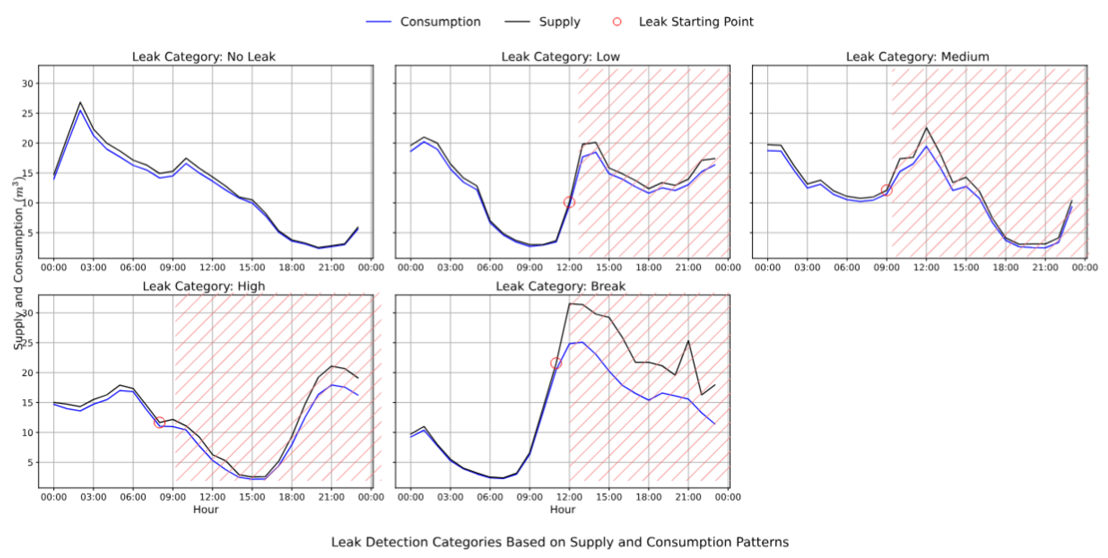
Different NRW-loss percentages are used to represent various leak severity levels [39]. As described in Section 4.3.3, the NRW-loss percentage is computed from the 24-hourly consumption–supply pairs. Out of a total of 1840 test samples per DMA, 920 samples exhibiting minimal or no NRW-loss are categorized as No-leak cases. The remaining 920 samples are evenly distributed for synthetic leak introduction. For each 24-hour sample, the leak onset is randomly positioned between the 8th and 12th hour to ensure sufficient pre-leak context for anomaly detection. From the onset time onward, the NRW-loss% is incrementally increased to reflect the desired severity level (as defined in Table 1), and the corresponding supply values are recalculated to simulate the synthetic leak scenario. The end-to-end system is evaluated using this dataset. Examples of supply and consumption under the influence of simulated leaks across different severity categories are showcased in Figure 7.
Figure 7.
Simulated leaks across different categories
- 2.
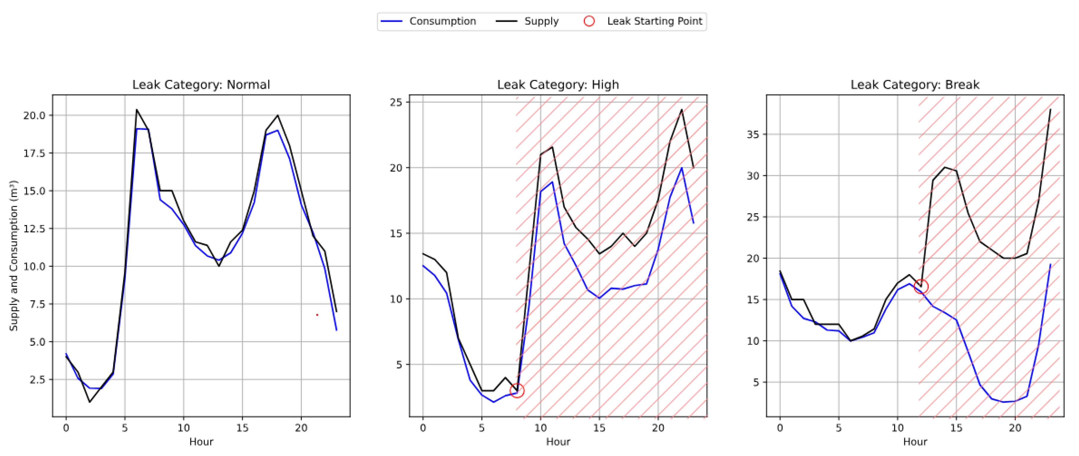
- Real-leak scenario datasets: Retrospective leak-annotations collected and confirmed from the utility are used for evaluations on real leak scenarios. Since our training process of regression models involve preprocessed and leak-corrected supply data, our evaluation of leakage detection does not conflict with standard definitions of machine learning evaluations. We selected 22 data-windows of real-leak events having the leak-onset within 8th-12th hour, from DMAs 01, 02, 03, 04, 05, 06, 07, 12, 13, 14, 15, 16, 17 and 21. These samples are assigned to class label of ’Leak’. Randomly 22 non-leak data-windows are selected with class-label ’No-leak’ for performing the evaluation of the leak-detection using classification metrics, as we intend to evaluate the false-positives and false-negatives. Analytical evaluation suggests that real-leaks comprise of only ’High’ and ’Break’ category. Real leaks of different categories are illustrated in Figure 8.
Figure 8.
Real leaks across different categories found in retrospective dataset
5.2. Experimental Overview
The experiments are conducted by orchestrating a modular pipeline on Databricks using the 13.3 LTS runtime framework. Training utilizes a Standard_D16ads_v5 compute node with 64 GB of memory and 16 cores. For inference, a Standard_D8ads_v5 compute node with 32 GB of memory is used. The system auto-scales the number of compute nodes between 4 and 12 based on computational consumption. The driver node, which acts as the central coordinator responsible for managing tasks and distributing work to the compute nodes, is configured identically to the compute nodes. The experimental setup is structured around two key components of the proposed framework: Offline Consumption-Supply Modeling, and Online Leak-Detection (refer to Figure 3).
For the comprehensive and robust evaluation of our proposed framework and each of its components, four experiments are conducted. The experiments are designed in two principal stages of our framework. First experiment is performed for a comprehensive and comparative evaluation of the consumption-to-supply regression ML models (henceforth labeled as Experiment I). The result of this experiment contributes with the ensemble artifacts as shown in the Figure 3. The performances of the regression models are assessed using the metrics defined in Section 4.5. The approach of one unified regression model in the model-ensemble for all DMAs is comparatively evaluated against the approach of DMA-specific regression models, without using one-hot encoding of DMA-identifiers, henceforth as Experiment II. The comparative evaluation of these two experiments suggests suitable regression approach in the consumption-to-supply estimation module. for the end-to-end leak detection pipeline.
Next, the leak-detection performance is assessed by employing two scoring mechanisms: MV-based metric-level ensembling (henceforth labeled as Experiment III) and PS-based metric-level ensembling (henceforth as Experiment IV). Leak detection performance is evaluated using the classification metrics discussed in Section 4.5.
5.3. Experimental Settings
Prepared dataset containing DMA-wise consumption and supply data from 21 DMAs are used for Experiment I. The dataset undergoes preprocessing steps including consumption-supply calculation, supply correction, min-max scaling, and DMA encoding. It is split into training (64%), validation (16%) and testing (20%) sets. Each DMA has 385 days of data, with 246 days for training, 61 for validation, and 78 for testing. Samples are generated with a 24-hour sliding window using a step size of 1, resulting in 7345 training, 1825 validation, and 1840 test samples per DMA. The hyperparameters of ML regression models are optimized using grid-search mechanism and showcased in Table 2.
Experiment II is conducted to understand the added-value of one-hot encoding of DMA identifiers. Instead of using one unified model for each DMA, resulting into total 4 regression models, DMA-specific models without requiring DMA-identifier encoding are trained and the performances are evaluated identically to Experiment I. Therefore this approach results in total 84 models. While in Experiment I, hyperparameters of SVR model was not optimized due to computational constraint, in Experiment II the hyperparameters are tuned for SVR as well. The hyperparameters of SVR in this ablation study are: C=0.1, epsilon=0.01, kernel=sigmoid, degree=4, gamma=0.01 and shrinking=True.
Identical dataset are used for evaluation of leak detection performance in Experiment III and IV. Simulated leak-scenario datasets (refer to Section 5.1) are used for the evaluation of leak-detection across all DMAs. However, real retrospective leaks are not available in all DMAs. Hence leak instances from 14 DMAs out of 21 DMAs are used in the evaluation. Final threshold operating point for leak/no-leak classification is varied from 0.2 to 0.7 to evaluate how classification performance is impacted for a certain operational threshold.
6. Results and Discussion
6.1. Consumption to Supply Estimation: Experiment I and II
Comparative Performance evaluation of individual regression models, i.e., XGBoost, MLP, RF and SVR, are conducted qualitatively and quantitatively. Please note that the performance evaluations of Experiment I and II are performed against the derived test dataset of the leak-corrected ground-truth supply data. Figure 9 illustrates examples of predicted supply in comparison to ground truth supply. In DMA 15, most models–except SVR–closely follow the observed supply trend. In DMA 05, while most models track the supply pattern reasonably well, the RF model shows noticeable deviations. In contrast, all models struggle to capture the supply dynamics in DMA 21 and DMA 12. Among them, SVR consistently underperforms, primarily due to the lack of hyperparameter tuning constrained by computational limitations.
Figure 10 shows that, in the DMA-specific modeling approach, all machine learning models effectively follow the supply pattern in DMA 15 and DMA 05. However, in DMA 21 and DMA 12, the models struggle to capture the supply behavior accurately. Among all models, MLP consistently shows the closest alignment with the observed supply, followed by XGBoost. In contrast, the RF model fails to capture the supply trends reliably, while SVR demonstrates better performance compared to Experiment I which is likely impacted by suboptimal hyperparameter tuning. The dynamics of the DMA 21 is exhibited due to the data quality of the district flow meters. For this DMA the district meter data is collected from SCADA (Supervisory Control And Data Acquisition) system’s flow sensors, than smart meters. The flow sensor measurements are usually snapshot-kind recorded measurements. This leads to clipped time-series characteristics when data is collected with coarser resolution.
However, the predicted supply, which apparently appears to be not following the stochastic pattern of supply, is actually the result of generalization attained by the model, which has reproduced the supposed diurnal pattern by using higher data quality of consumption data. The anomalous spike appearing in DMA 12 between 13:00 and 15:00 on 30-05 is a physical effect of momentary valve opening, as informed by the utility. Such characteristics actually resembles to a leak-like pattern within small time-span. Hence, the regression models have captured the supposed normal supply pattern, and capturing the deviation within the mentioned time-frame is teh sole objective of our proposed framework.
The results in the box plots (Figure 11) along with Table 3 clearly demonstrate XGBoost’s superior performance, consistently achieving the lowest median MAPE and RMSE with minimal variability. MLP remains competitive, showing moderate error rates and variability. SVR achieves lower error-range in Experiment II, indicating effective hyperparameter tuning. Conversely, RF shows higher error values and greater variability, suggesting limited robustness in modeling Consumption-supply dynamics.
Apart from SVR, performances of all the regression models suggest that the regression modeling approach of Experiment I results in lower mean and standard deviation of performance compared to their corresponding counterpart in Experiment II, i.e. DMA-specific modeling. Hence, the modeling approach of Experiment I is used in the end-to-end leak-detection pipeline.
XGBoost demonstrates strong consistency between the unified (Experiment I) and DMA-specific (Experiment II) frameworks, achieving nearly identical accuracy and error dispersion. This reflects its ability to capture both global and local consumption–supply relationships effectively through optimal tree partitioning and robust regularization. The MLP performs comparably across both setups, showing slightly lower mean error in the unified model but with higher variability. The unified framework benefits from larger aggregated data, though heterogeneous DMA patterns introduce instability in training and convergence. SVR exhibits the largest framework-dependent differences, performing significantly worse in the unified setting due to the absence of DMA-specific hyperparameter tuning. Its results highlight SVR’s sensitivity to parameter optimization rather than structural limitations of the modeling framework. RF performs similarly across both experiments, consistently lagging behind other models. Its bagging ensemble structure, while robust to noise, weakens fine-grained spatial relationships and lacks the adaptive capacity to model complex nonlinear dependencies.
Overall, the unified modeling framework achieves accuracy comparable to the per-DMA approach with substantially lower computational and maintenance overhead—only four models versus eighty-four—making it more scalable and operationally efficient for large-scale deployment. Most importantly, the performance evaluation shows the ability of the unified-modeling approach in Experiment I to capture DMA-specific Consumption-supply dynamics with the help of one-hot encoding of DMA names.
6.2. Leak Detection: Experiment III and IV
Leak detection performance is assessed both qualitatively and quantitatively in Experiments III and IV. The qualitative analysis visualizes how the predicted supply from different regression models deviates from the observed supply when trained using DMA-specific Consumption data and encoded DMA identifiers. Figure 12 illustrates examples of mentioned deviation starting from leak-onset in the simulated dataset, whereas Figure 13 showcases the pattern-deviations of observed supply data with respect to predicted supply in real retrospective dataset.
In both simulated and real leak datasets, supply and consumption show strong initial correlation across DMAs (Figure 12 and Figure 13). In the simulated case, supply aligns with consumption until a leak is introduced—at the 11th hour for DMA 18 and DMA 08—after which observed supply (black line) exceeds consumption (blue line), indicating water loss. Similarly, in the real dataset, divergence begins at the 12th hour, showcasing an actual leak. In both cases, estimated supply (dotted lines) continues to track consumption, highlighting the models’ ability to detect leaks via deviation analysis.
Quantitative evaluation of Experiment III and IV are conducted with the help of Confusion matrices, ROC-curve with AUC-scores and standard classification metrics mentioned in the Section 4.5.
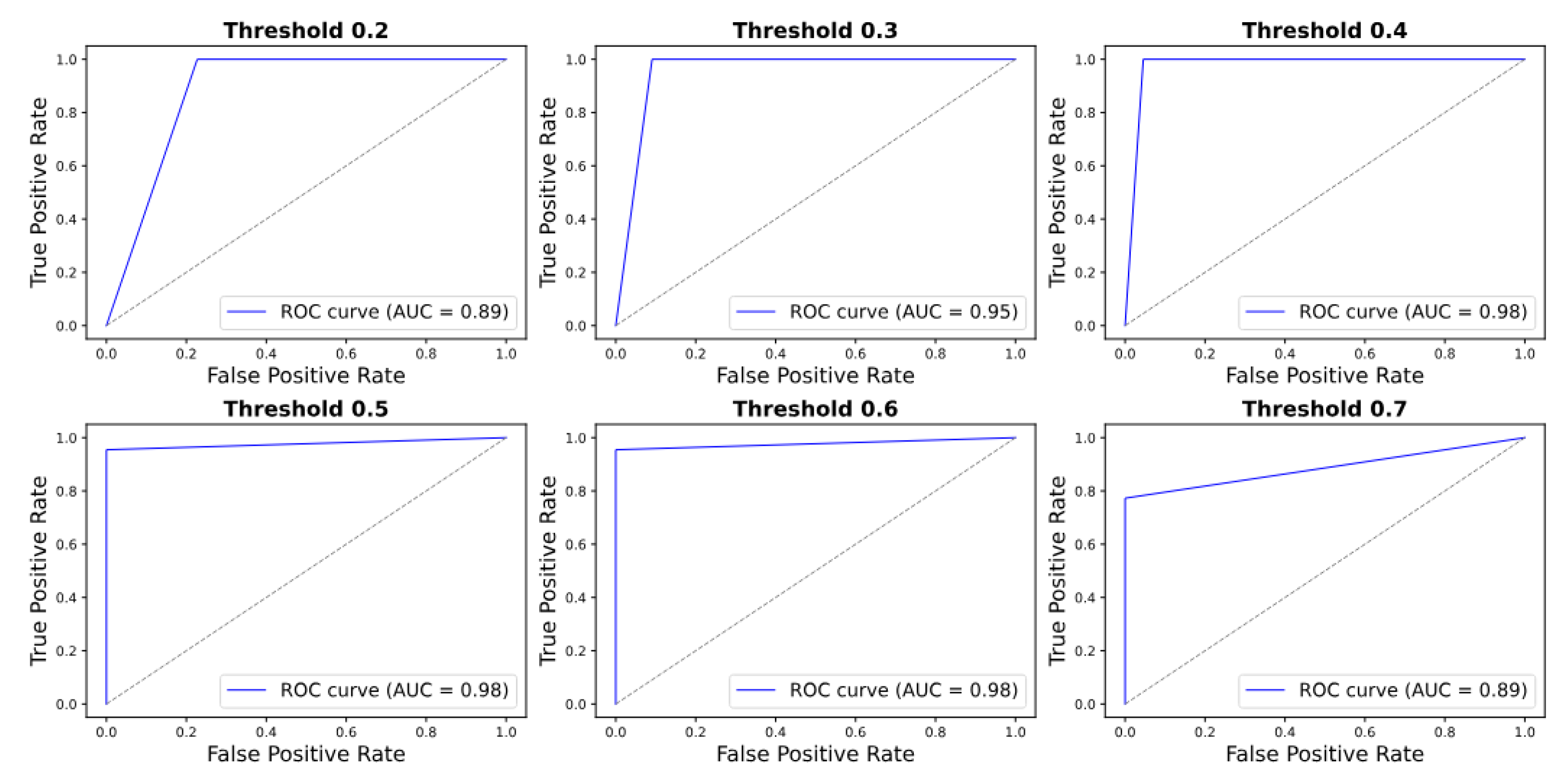
The confusion matrix analysis (Figure 14) shows how threshold adjustments affect leak detection performance. In the simulated case, a low threshold (0.2) detects most leaks (18097) and no-leaks (14729) but results in 4590 false alarms. Raising the threshold to 0.7 reduces false alarms to 443 but increases missed leaks to 5017. At the balanced threshold of 0.5, the model correctly identifies 16,496 leaks and 18,396 no-leaks, with 923 false alarms and 2,830 missed leaks. Whereas in the real dataset (Figure 15), at a 0.2 threshold, the model detects 22 leaks and 19 no-leaks, with 3 false alarms. From thresholds 0.3 to 0.7, the model produces 0 false alarms. However, missed leaks increase slightly–from none at 0.3 to 2 at 0.7.
The ROC curve analysis (Figure 16 and Figure 17) demonstrates consistent model performance across thresholds. For the simulated dataset, the AUC peaks at 0.91 for thresholds of 0.3 and 0.4, with a marginal decrease to 0.86 at 0.7. In the real dataset, the AUC remains exceptionally high—reaching 1.00 at 0.3 and 0.4 and exceeding 0.92 for all thresholds—indicating robust and reliable classification.
The classification report for the simulated leak dataset (Table 4) shows that the thresholds 0.3 and 0.4 offer the best balance, with 0.91 accuracy and F1 scores for both classes. From threshold 0.2 to 0.7, leak precision rises from 0.80 to 0.97, while recall drops from 0.94 to 0.74. No-leak precision falls from 0.92 to 0.79, and recall increases from 0.76 to 0.98, reflecting a trade-off where higher thresholds reduce false alarms but increase missed leaks.
For the real leak dataset (Table 5) enhanced performance is observed. At the 0.3 and 0.4 thresholds, all metrics reach 1.00. At threshold 0.2, accuracy is 0.93 with leak precision at 0.88 and no-leak precision at 1.00. Above 0.4, leak recall slightly falls to 0.91 at 0.7, while precision remains high (0.92–1.00), maintaining reliable detection with minimal false alarms.
In case of Experiment IV, performances are illustrated as follows for PS-approach. The confusion matrices for the simulated dataset highlight a trade-off between leak detection and false alarms as the threshold increases (refer to Figure 18). At 0.2, the model detects 18560 leaks and 14535 no-leaks, but with 4784 false alarms and 766 missed leaks. As the threshold rises to 0.7, false alarms drop to 152, while missed leaks increase to 7308.
In the real dataset (Figure 19), the performances using PS approach are observed as follows. At 0.2, it detects all 22 leaks with 5 false alarms. By threshold 0.4, false alarms drop to 1 with perfect leak detection. At 0.5–0.6, one leak is missed and no false alarms occur. At 0.7, 5 leaks are missed, with 17 detected and no false alarms.
At lower thresholds (e.g., 0.2), both MV and PS focus on detecting every possible leak, achieving perfect or near-perfect recall on the real dataset and around 0.9 on the simulated one. However, this strong sensitivity also increases false positives, especially in the simulated data, which lowers precision. In contrast, the non-leak class shows high precision but lower recall, indicating that the models become biased towards when labeling samples as leaks than non-leak while prioritizing leak detection.
When the threshold increases to 0.3–0.4, both methods achieve a better balance between precision and recall. False positives drop sharply, and F1-scores for leak and non-leak classes stabilize around 0.9 in the simulated dataset. The ROC-AUC remains strong (about 0.9), and in the real dataset, both MV and PS achieve almost perfect classification, with precision, recall, and F1-scores reaching 1.00. This indicates that both methods perform very reliably under real dataset where the distinction between leak and non-leak patterns is clearer due to only high severity leak-categories being present in the samples.
Figure 20.
Exp IV: PS Performance Evaluation via ROC Curves (Simulated Leaks)
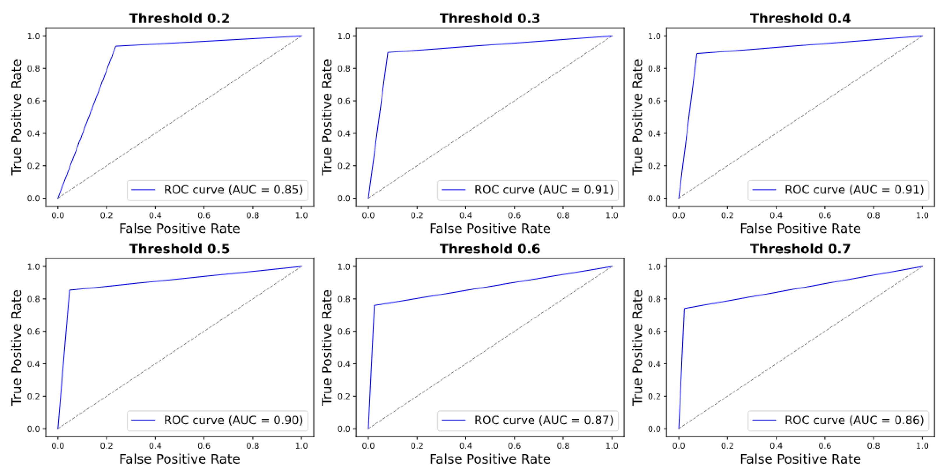
Figure 21.
Exp IV: PS Performance Evaluation via ROC Curves (Real Leaks)
At higher thresholds (above 0.5), the models become more conservative, favoring precision over recall. Leak precision rises above 0.95, while recall decreases below 0.8, showing that the models aim to reduce false alarms but may miss some true leaks. Despite this trade-off, non-leak recall remains high (around 0.95–0.98), and real-world results continue to be stable – precision stays perfect, and recall decreases only slightly. Hence the comprehensive analysis of performance in both the experiments – Experiment III and IV illustrates the traditional trade-off between sensitivity and specificity of anomaly detection. The results showcase the optimal operating point where the balance can be obtained. The higher resilience in performance observed in case of real data is due to only ’High’ and ’Break’ category leaks being present in the dataset, where the deviation pattern is clearer.

Table 6.
Exp IV: PS Classification Report (Simulated Leaks)
| Threshold | Class | Precision | Recall | F1-score | Accuracy | Support |
|---|---|---|---|---|---|---|
| 0.2 | No Leak | 0.95 | 0.75 | 0.84 | 0.86 | 19319 |
| Leak | 0.80 | 0.96 | 0.87 | 19326 | ||
| 0.3 | No Leak | 0.93 | 0.85 | 0.89 | 0.89 | 19319 |
| Leak | 0.86 | 0.93 | 0.90 | 19326 | ||
| 0.4 | No Leak | 0.89 | 0.92 | 0.91 | 0.90 | 19319 |
| Leak | 0.92 | 0.89 | 0.90 | 19326 | ||
| 0.5 | No Leak | 0.85 | 0.96 | 0.90 | 0.90 | 19319 |
| Leak | 0.96 | 0.83 | 0.89 | 19326 | ||
| 0.6 | No Leak | 0.78 | 0.98 | 0.87 | 0.85 | 19319 |
| Leak | 0.98 | 0.72 | 0.83 | 19326 | ||
| 0.7 | No Leak | 0.72 | 0.99 | 0.84 | 0.81 | 19319 |
| Leak | 0.99 | 0.62 | 0.76 | 19326 |
Table 7.
Exp IV: PS Classification Report (Real Leaks)
| Threshold | Class | Precision | Recall | F1-score | Accuracy | Support |
|---|---|---|---|---|---|---|
| 0.2 | No Leak | 1.00 | 0.77 | 0.87 | 0.89 | 22 |
| Leak | 0.81 | 1.00 | 0.90 | 22 | ||
| 0.3 | No Leak | 1.00 | 0.91 | 0.95 | 0.95 | 22 |
| Leak | 0.92 | 1.00 | 0.96 | 22 | ||
| 0.4 | No Leak | 1.00 | 0.95 | 0.98 | 0.98 | 22 |
| Leak | 0.96 | 1.00 | 0.98 | 22 | ||
| 0.5 | No Leak | 0.96 | 1.00 | 0.98 | 0.98 | 22 |
| Leak | 1.00 | 0.95 | 0.98 | 22 | ||
| 0.6 | No Leak | 0.96 | 1.00 | 0.98 | 0.98 | 22 |
| Leak | 1.00 | 0.95 | 0.98 | 22 | ||
| 0.7 | No Leak | 0.81 | 1.00 | 0.9 | 0.89 | 22 |
| Leak | 1.00 | 0.77 | 0.87 | 22 |
6.2.1. MV vs PS
Both MV and PS exhibit strong overall agreement in performance across simulated and real datasets but differ in how they balance precision and recall at varying thresholds.
At lower thresholds (0.2–0.4), MV provides more stable and balanced performance, maintaining higher leak precision and comparable recall, while PS favors higher sensitivity at the cost of more false positives. In the real dataset, both methods achieve perfect leak recall, though MV consistently attains higher precision and F1-scores, reflecting fewer false alarms and better overall classification balance.
As the threshold increases (0.5–0.7), MV demonstrates greater robustness and slower performance degradation compared to PS. MV sustains higher precision and accuracy with moderate recall loss, whereas PS becomes increasingly conservative—boosting leak precision but sharply reducing recall and overall F1-scores. On real data, MV retains its stability even at higher thresholds, achieving balanced precision–recall values and fewer false detections than PS.
Overall, MV achieves a superior trade-off between sensitivity and specificity across datasets, offering more consistent and dependable performance. PS performs competitively when minimizing false positives is the top priority, but MV’s balanced and resilient behavior makes it more suitable for practical leak detection scenarios where missing true leaks is costlier than occasional false alarms.
6.2.2. Optimal Threshold for Leak Decision
The leak decision threshold plays a critical role in shaping the performance of both the MV and PS strategies. Lower values of cause the system to classify even mild deviations as leaks. With lower , recall is high because nearly all leak events are detected; however, the rate of false positives increases, particularly in the simulated dataset where leak signatures may overlap more strongly with background variability. In contrast, the real dataset exhibits better class separability, resulting in fewer false alarms at comparable threshold levels.
As the threshold is increased into a mid-range (), both MV and PS achieve a more balanced trade-off between sensitivity and reliability. In this range, leak precision and recall remain simultaneously high, and the number of false positives decreases substantially. For the real dataset in particular, this threshold region yields near-perfect performance, as reflected in high F1-scores and ROC-AUC values approaching 0.98.
Further increasing the threshold () leads to a more conservative decision rule. Precision remains high because only the most pronounced anomalies exceed the threshold, but recall decreases as smaller or short-duration leaks are not detected. This results in fewer false positives but a reduction in overall discriminative balance.
In summary, threshold selection should align with operational priorities: lower thresholds when maximizing leak detection is critical, mid-range thresholds when balanced performance is desired, and higher thresholds when minimizing false alarms is more important than detecting every leak event.
6.3. Impact of Ensembling on Leak Detection Accuracy
The impact of ensembling multiple regression models can be assessed by taking into account predicted supply of individual regression models as the basis for deviation analysis from observed supply. This analysis is carried out on simulated dataset as leaks of various categories are present in simulated-leak dataset, in contrast to the real-leak dataset. As shown in Figure 22, performance across leak categories varied significantly when using individual models, particularly for medium and low-severity leaks. All models demonstrated strong performance in detecting Break-type leaks (scores: 0.91–1.00) and reliably identified Normal operating conditions, with classification scores in the range of 0.88–0.93.
However, their effectiveness dropped notably for other critical categories. The RF model scored as low as 0.56 in High leaks, and RF and SVR scored 0.33 and 0.68 in Medium leaks, respectively. The Low leaks were the most difficult to detect (the highest RF was only 0.20 and the highest SVR was only 0.51). These inconsistencies underscore the limitations of relying solely on individual models, especially their tendency to underperform on less frequent or more ambiguous leak types. These findings are corroborated by the individual DMA-level analysis (Figure 22), where, as discussed in Section 6.1, MLP and XGBoost emerged as the most reliable models for estimating water supply, directly enhancing leak detection capabilities. Both models consistently achieved over 0.90 accuracy in detecting leaks across most DMAs, demonstrating strong generalization to underlying supply patterns. In contrast, RF performed poorly, failing to exceed 0.81 accuracy in most DMAs (except DMA 04), while SVR, though more competitive than RF, achieved an average accuracy of 0.82—slightly lower than the 0.88 average attained by MLP and XGBoost. These variations suggest that some models are more sensitive to data quality and local noise at the DMA level, resulting in less stable and less reliable detection performance.
But a key observation is that, for DMA 12, 19, 21 and 22, higher classification accuracy is achieved using the prediction of SVR compared to that from XGBoost. This highlights the complementary effect of integrating another model’s opinion through an ensembling mechanism, to overcome limitation of a model whose performance can deviate in a different data scenario. Thus, the ensembling process increases confidence and robustness in classification by incorporating predictions from other models. Furthermore, the limitations observed across both leak categories and individual DMAs are effectively addressed by the ensembling approach, which integrates outputs from multiple models through metric-level fusion (MV and PS) and model-level weighting based on accuracy. This strategy leverages the strengths of each base learner while mitigating their individual weaknesses.
After applying the ensemble method (Figure 23), the model exhibited substantially more stable and reliable performance across all leak categories. It consistently maintained near-perfect accuracy (>0.98) in detecting Break leaks across all threshold settings, ensuring dependable recognition of the most severe failures. Detection of high severity leaks also improved significantly, with accuracy never falling below 0.86—even as the decision threshold increased from 0.2 to 0.7. Although this reflects a slight trade-off between sensitivity and specificity, the ensemble preserved high detection rates for critical leak events. Classification of Normal conditions showed notable improvement as well. Accuracy increased from 0.76 at threshold 0.2 to above 0.92 at higher thresholds, suggesting that the ensemble becomes more confident and specific in identifying normal operations as the decision boundary tightens. However, this improved specificity came at the expense of sensitivity to less severe leaks. The Medium category remained relatively stable (>0.80) up to threshold 0.5 but declined below 0.70 beyond that. The Low category was the most sensitive to threshold changes, with accuracy dropping from 0.85 at threshold 0.2 to 0.46 at threshold 0.7.
Overall, these findings underscore a critical insights for ensemble model design. Low-category leaks are inherently more difficult to detect, both before and after ensembling. The highest individual accuracy for the Low category leaks before ensembling was 0.79, achieved by the MLP model. With ensembling, the maximum classification accuracy for the Low category reached only 0.85, and this came at the cost of reducing the accuracy for the Normal class to 0.76. Therefore, in practical deployment, a threshold of 0.76 appears to be the optimal trade-off point, as it preserves reasonable sensitivity to low-severity leaks without compromising classification of other categories.
Altogether, these results demonstrate the tolerance of the ensemble approach against model-dependent sensitivities and noisy measurements. It reduces performance fluctuation among the leak categories and DMAs and enhances overall reliability.
6.4. Kalman-View and Neural Network MoE-View of the Proposed Framework
The proposed framework can be understood as an innovation-based monitoring system, similar in spirit to Kalman filtering. Each regression model acts as a predictor of the expected DMA supply under normal hydraulic behavior. The deviation between predicted and observed supply forms an innovation signal, whose statistical properties rather than raw residuals are monitored to identify deviations from nominal operation. Under normal conditions, these innovation statistics remain stable and consistent with their training-time behavior.
When a new leak emerges, the relationship between consumption and supply changes, and the innovation statistics shift accordingly. The metric-level fusion acts as an innovation gate, deciding whether each model finds its innovation inconsistent with expected behavior. The model-level weighted fusion then combines these innovation evidences, analogous to reliability-weighted multi-model filtering. Finally, thresholding the aggregated anomaly score corresponds to a hypothesis test on the innovation process, where exceeding the threshold indicates a statistically significant departure from nominal hydraulics and therefore a potential leak. In this sense, the entire pipeline behaves as a Kalman-style innovation detector, where expected behavior comes from trained regression models. Here the deviations are characterized through innovation statistics, and the ensemble process provides robust decision making.
The framework can also be interpreted as a Mixture-of-Experts (MoE) architecture. Each regression model acts as an expert that estimates supply from consumption for a DMA. Instead of learning neural hidden layers, the framework computes simple statistical measures describing how well each expert’s prediction matches the observed supply. These statistics act as a lightweight representation of residual behavior.
A deterministic fusion rule converts the metric vector into a per-model anomaly score, and the RMO weights serve as fixed attention coefficients, emphasizing experts that historically predicted reasonably for the DMA. The weighted combination of expert scores then produces a single anomaly score, which is finally thresholded to produce the leak decision.
Viewed this way, the pipeline resembles a transparent, hand-crafted mixture-of-experts model, where each expert contributes according to its reliability and the “gating mechanism” is implemented through RMO weights rather than learned parameters.
7. Conclusion
The proposed machine learning framework provides a fast, automated, and scalable solution for data-driven leak detection across multiple water utilities. To the best of our knowledge, this is the first study to employ a regression- and ensemble-based methodology for detecting leaks in water distribution networks using smart meter–derived, DMA-specific demand and supply data. Based on the triggers generated from such system, a limited-area-scoped hydraulic-simulation based optimization can be executed to find the leak at pipe-level which is a significant reduction of computational burden. The whole system can be designed for deployment with minimal human intervention as a data-driven automated framework, ensuring consistency and reproducibility across all stages – from data preprocessing to model training and inference. The framework demonstrates the capability to identify leaks within 8–12 hours of onset, achieving high detection accuracy across varying leak magnitudes. The added value of ensemble learning is clearly shown by the improved detection performance over the same from the predictions of individual regression models.
The first part of the study assessed multiple regression models for accurate estimation of DMA-level water supply, informing both model choice and the decision between unified and DMA-specific modeling strategies. Unified modeling, incorporating DMA identifiers, proved most effective overall, providing a balance between predictive accuracy and scalability. Although DMA-specific models occasionally yielded marginally higher accuracy, the associated increase in complexity outweighed their benefits.
The second component of the framework addressed unsupervised leak detection by analyzing deviations between predicted and observed supply. The ensemble of multiple regression models, integrating both metric-level and model-level ensembling, achieved strong leak detection performance without requiring labeled data, thereby enabling scalable, near-real-time detection across diverse operational contexts. While evaluating individual regression model prediction-based leak detection, XGBoost and MLP consistently exhibited robust performance offering stability. However the SVR model showed complementary performance in specific DMAs when used for individual regression-model–based leak detection. This is a strong evidence of using opinion of multiple regression models and metrics to achieve stable performance in leak-detection.
The consistently strong performance of MLP across multiple DMAs and leak categories suggests the potential of developing a single, advanced neural network model capable of substituting the entire ensemble framework. Future work will explore this possibility using deep neural architectures for end-to-end leak detection. Additionally, the simulated leak dataset may serve as a basis for training supervised classification models to learn the decision boundary between leak and no-leak conditions, rather than relying on statistical metric distributions. Finally, evaluating the proposed framework in alternative utility settings—particularly those exhibiting stronger non-stationary behavior in demand due to climatic influences—would further establish its generalizability and operational robustness.
Author Contributions
Conceptualization, S.C.; methodology, S.C., S.G., D.T.,; software, S.G., S.C.; validation, S.C., S.G., S.B., A.R., M.A., K.S.; formal analysis, S.G., S.C.; investigation, S.G., S.C.; resources, M.A., K.S.; data curation, M.A., S.G.; writing—original draft preparation, S.C.; writing—review and editing, S.B., A.R., S.G., K.S., M.A., D.T. ; visualization, S.G., S.C.; supervision, S.C., S.B., A.M., D.T., K.S.; project administration, S.C., K.S.; funding acquisition, K.S., All authors have read and agreed to the published version of the manuscript.
Funding
This research was funded by Diehl Metering GmbH.
Data Availability Statement
The input data for the experiments are confidential
Acknowledgments
We acknowledge the support of cloud infrastructure for computations at-scale provided by Diehl Metering GmbH. During the preparation of this manuscript, the authors used LLM, namely, ChatGPT 5.1 for the purposes of sentence and language refinements. The authors have reviewed and edited the output and take full responsibility for the content of this publication.
Conflicts of Interest
The authors declare no conflicts of interest.
Abbreviations
The following abbreviations are used in this manuscript:
| AE | Autoencoder |
| AMI | Automated Metering Infrastructure |
| AUC | Area Under Curve |
| CDCGAN | Conditional Deep Convolutional Generative Adversarial Network |
| CNN | Convolutional Neural Network |
| COPOD | Copula-based Outlier Detection |
| DMA | District Metered Area |
| DS | Data Science |
| DT | Decision Tree |
| ECOD | Empirical Cumulative Distribution Functions |
| EPANET | Environmental Protection Agency’s Network Analysis Tool |
| FPR | False Positive Rate |
| GIS | Geographic Information System |
| IMM | Interactive Multiple Model |
| IWA | International Water Association |
| LTS | Long Term Support |
| MAPE | Mean Absolute Percentage Error |
| MDM | Meter Data Management |
| MEL | Multi Strategy Ensemble Learning |
| ML | Machine Learning |
| MLP | Multi-Layer Perceptron |
| MMD | Metric-Model-DMA |
| MoE | Mixture-of-Experts |
| MSE | Mean Squared Error |
| MV | Majority Voting |
| NB | Naïve Bayes |
| NRW | Non Revenue Water |
| PCA | Principal Component Analysis |
| PS | Proportional Scoring |
| RF | Random Forest |
| RMSE | Root-Mean-Squared Error |
| ROC | Region Of Convergence |
| RMO | Regression Model Opinion |
| SCADA | Supervisory Control And Data Acquisition |
| SVM | Support Vector Machine |
| SVR | Support Vector Regression |
| TPR | True Positive Rate |
| WDN | Water Distribution Network |
| WDS | Water Distribution System |
| XGBoost | Extreme Gradient Boosting |
Appendix A.
Appendix A.1. Boundedness and Probabilistic Interpretation of the Anomaly Score
This appendix establishes two properties of the proposed anomaly score: (i) the ensemble anomaly score obtained from both Majority Voting (MV) and Proportional Scoring (PS) is always bounded in the interval , and (ii) the final anomaly score admits a probabilistic interpretation as an empirical estimate of the likelihood of a leakage event.
Metric-Level Anomaly Indicators
For a given DMA d, regression model m, statistical metric (refer to equation 20) , and sample s, the metric-level anomaly indicators are defined as
where a value of 1 denotes violation of the corresponding metric threshold (anomaly detected), and 0 denotes normal behavior (refer to equation 25). Each metric therefore produces a hard binary anomaly decision.
Model-Level Anomaly Scores
Using the metric-level indicators, two types of model-level anomaly scores are constructed. We can rewrite equation 28 and equation 29 as,
-
Majority Voting (MV):where is the number of statistical metrics. Hence, the MV score is binary by construction.
-
Proportional Scoring (PS):Since this score is the arithmetic mean of V binary indicators, it satisfies
Model-Level Ensembling
The model-level anomaly scores are fused across M number of regression models using the RMO weights, which can be rewritten from equations 30 and 31:
where the RMO weights are defined as
Assumptions: The boundedness and probabilistic interpretation rely on the following assumptions:
- (A1) Metric-level anomaly indicators are binary:
- (A2) MAPE values are bounded:which ensures
- (A3) The total model weight is strictly positive:
Boundedness of the Ensemble Anomaly Score: From (A1), the MV score satisfies
and from the definition of PS,
Since the ensemble fusion is performed as a weighted average using non-negative weights , the ensemble score can be rewritten using normalized weights
which satisfy
The ensemble anomaly score therefore takes the form
which is a convex combination of values lying in . Hence, the final ensemble anomaly score is guaranteed to satisfy
Probabilistic Interpretation
Each metric-level indicator can be interpreted as a realization of a Bernoulli random variable representing the detection of a leak by metric j.
For Proportional Scoring (PS), the model-level score
is the arithmetic mean of multiple Bernoulli trials and therefore serves as an empirical estimate of the average leak probability across the V statistical metrics for model m.
For Majority Voting (MV), the model-level score
represents a hard binary decision that can be interpreted as a thresholded estimate of the underlying leak probability, where a leak is declared if the majority of metric-level Bernoulli trials indicate anomaly.
At the ensemble level, the final anomaly score,
is a convex mixture of model-wise probability estimates (for PS) or binary probability surrogates (for MV). This corresponds to a standard mixture-of-experts formulation. Consequently, the final anomaly score admits a probabilistic interpretation as an empirical estimate of the likelihood of leakage at DMA d and sample s.
References
- Lambert, A.O.; Brown, T.G.; Takizawa, M.; Weimer, D. A review of performance indicators for real losses from water supply systems. Journal of Water Supply: Research and Technology-Aqua 1999, 48, 227–237. Available online: https://iwaponline.com/aqua/article-pdf/48/6/227/134471/227.pdf. [CrossRef]
- Barton, N.A.; Farewell, T.S.; Hallett, S.H.; Acland, T.F. Improving pipe failure predictions: Factors affecting pipe failure in drinking water networks. Water Research 2019, 164, 114926. [Google Scholar] [CrossRef]
- Agency, D.E.P. Preventing water loss. Website 2024. [Google Scholar]
- Liemberger, R.; Wyatt, A. Quantifying the global non-revenue water problem. Water Supply 2018, 19, 831–837. Available online: https://iwaponline.com/ws/article-pdf/19/3/831/592655/ws019030831.pdf. [CrossRef]
- Shao, Y.; Yu, Y.; Yu, T.; Chu, S.; Liu, X. Leakage Control and Energy Consumption Optimization in the Water Distribution Network Based on Joint Scheduling of Pumps and Valves. Energies 2019, 12. [Google Scholar] [CrossRef]
- Dastpak, P.; Sousa, R.L.; Dias, D. Soil Erosion Due to Defective Pipes: A Hidden Hazard Beneath Our Feet. Sustainability 2023, 15. [Google Scholar] [CrossRef]
- Ribeiro, A.; Haghi, A. Smart Management of Water Loss at the District Metered Areas (DMA); 2024; pp. 29–42. [Google Scholar] [CrossRef]
- Mix, N.; Lai, A.; Thompson, K.; Seachrist, S. Advanced Metering Infrastructure: Reducing Water Loss, Improving Security, and Enhancing Resiliency. Journal - American Water Works Association 2020, 112, 38–49. [Google Scholar] [CrossRef]
- Huang, Y.; Zheng, F.; Kapelan, Z.; Savic, D.; Duan, H.F.; Zhang, Q. Efficient Leak Localization in Water Distribution Systems Using Multistage Optimal Valve Operations and Smart Demand Metering. Water Resources Research 2020, 56, e2020WR028285. Available online: https://agupubs.onlinelibrary.wiley.com/doi/pdf/10.1029/2020WR028285. [CrossRef]
- Lambert, A. International Report: Water losses management and techniques. Water Supply 2002, 2, 1–20. Available online: https://iwaponline.com/ws/article-pdf/2/4/1/407625/1.pdf. [CrossRef]
- Kanakoudis, V.; Tsitsifli, S.; Cerk, M.; Banovec, P.; Samaras, P.; Zouboulis, A. Basic Principles of a DSS Tool Developed to Prioritize NRW Reduction Measures in Water Pipe Networks. Water Quality Exposure and Health 2015, 7, 39–51. [Google Scholar] [CrossRef]
- Cassidy, J.; Barbosa, B.; Damião, M.; Ramalho, P.; Ganhão, A.; Santos, A.; Feliciano, J. Taking water efficiency to the next level: digital tools to reduce non-revenue water. Journal of Hydroinformatics 2020, 23, 453–465. Available online: https://iwaponline.com/jh/article-pdf/23/3/453/892596/jh0230453.pdf. [CrossRef]
- Feliciano, J.; Almeida, R.; Santos, A.; Ramalho, P.; Ganhão, A.; Covas, D.; Alegre, H. Assessing human resources renovation needs in water utilities. Water Practice and Technology 2016, 11, 728–735. Available online: https://iwaponline.com/wpt/article-pdf/11/4/728/381265/wpt0110728.pdf. [CrossRef]
- Hu, Z.; Chen, B.; Chen, W.; Tan, D.; Shen, D. Review of model-based and data-driven approaches for leak detection and location in water distribution systems. Water Supply 2021, 21, 3282–3306. Available online: https://iwaponline.com/ws/article-pdf/21/7/3282/1104597/ws021073282.pdf. [CrossRef]
- Yang, X.; Howley, E.; Schukat, M. ADT: Agent-based Dynamic Thresholding for Anomaly Detection. arXiv 2023, arXiv:2312.01488. [Google Scholar] [CrossRef]
- Platte, T. Evaluation of the uncertainty of measurement for a dynamic calibration approach for pressure sensors. Measurement: Sensors 2021, 18, 100252. [Google Scholar] [CrossRef]
- Wu, Y.; Liu, S.; Kapelan, Z. Addressing data limitations in leakage detection of water distribution systems: Data creation, data requirement reduction, and knowledge transfer. Water Research 2024, 267, 122471. [Google Scholar] [CrossRef]
- Rajan, G.; Li, S. A Systematic Literature Review on Flow Data-Based Techniques for Automated Leak Management in Water Distribution Systems. Smart Cities 2025, 8. [Google Scholar] [CrossRef]
- Sousa, D.P.; Du, R.; Mairton Barros da Silva, J., Jr.; Cavalcante, C.C.; Fischione, C. Leakage detection in water distribution networks using machine-learning strategies. Water Supply 2023, 23, 1115–1126. Available online: https://iwaponline.com/ws/article-pdf/23/3/1115/1261125/ws023031115.pdf. [CrossRef]
- Aravind Britto, K.; Prasad, D.; Ragavendiran, S.D.P.; Shreepad, S.; Singh, N.K.; Bhowmick, A.; Siva Ramkumar, M. Supervised Learning Algorithm for Water Leakage Detection through the Pipelines. In Proceedings of the 2022 3rd International Conference on Smart Electronics and Communication (ICOSEC), 2022; pp. 1263–1269. [Google Scholar] [CrossRef]
- Ravichandran, T.; Gavahi, K.; Ponnambalam, K.; Burtea, V.; Mousavi, S.J. Ensemble-based machine learning approach for improved leak detection in water mains. Journal of Hydroinformatics 2021, 23, 307–323. Available online: https://iwaponline.com/jh/article-pdf/23/2/307/859146/jh0230307.pdf. [CrossRef]
- Mashhadi, N.; Shahrour, I.; Attoue, N.; El Khattabi, J.; Aljer, A. Use of Machine Learning for Leak Detection and Localization in Water Distribution Systems. Smart Cities 2021, 4, 1293–1315. [Google Scholar] [CrossRef]
- Yu, H.; Lin, S.; Zhou, H.; Weng, X.; Chu, S.; Yu, T. Leak detection in water distribution networks based on deep learning and kriging interpolation method. AQUA - Water Infrastructure, Ecosystems and Society 2024, 73, 1741–1753. Available online: https://iwaponline.com/aqua/article-pdf/73/8/1741/1468952/jws2024184.pdf. [CrossRef]
- Lochan Basnet, R.R. SUPERVISED MACHINE LEARNING MODELS FOR LEAK DETECTION IN WATER DISTRIBUTION SYSTEMS. 2nd International Joint Conference on Water Distribution Systems Analysis and Computing and Control in the Water Industry, 2022. [Google Scholar] [CrossRef]
- Fan, X.; Yu, X.B. An innovative machine learning based framework for water distribution network leakage detection and localization. Structural Health Monitoring 2022, 21, 1626–1644. [Google Scholar] [CrossRef]
- Rajabi, M.M.; Komeilian, P.; Wan, X.; Farmani, R. Leak detection and localization in water distribution networks using conditional deep convolutional generative adversarial networks. Water Research 2023, 238, 120012. [Google Scholar] [CrossRef]
- Aghashahi, M.; Sela, L.; Banks, M.K. Benchmarking dataset for leak detection and localization in water distribution systems. Data in Brief 2023, 48, 109148. [Google Scholar] [CrossRef]
- Berardi, L.; Giustolisi, O. Calibration of Design Models for Leakage Management of Water Distribution Networks. Water Resources Management 2021, 35. [Google Scholar] [CrossRef]
- Santos-Ruiz, I.; López-Estrada, F.R.; Puig, V.; Valencia-Palomo, G.; Hernández, H.R. Pressure Sensor Placement for Leak Localization in Water Distribution Networks Using Information Theory. Sensors 2022, 22, 443. [Google Scholar] [CrossRef]
- Truong, H.; Tello, A.; Lazovik, A.; Degeler, V. DiTEC-WDN: A Large-Scale Dataset of Hydraulic Scenarios across Multiple Water Distribution Networks. arXiv 2025, arXiv:cs. [Google Scholar] [CrossRef]
- Fuertes, P.C.; Alzamora, F.M.; Carot, M.H.; Campos, J.A. Building and exploiting a Digital Twin for the management of drinking water distribution networks. Urban Water Journal 2020, 17, 704–713. [Google Scholar] [CrossRef]
- Yu, Z.; Ye, Z.; Zheng, F.; Zhang, Y.; Shen, Y. Automatic detection of water pipeline leakage via unsupervised learning applied on ground penetrating radar data. Journal of Hydroinformatics 2024, 26. [Google Scholar] [CrossRef]
- Leonzio, D.U.; Bestagini, P.; Marcon, M.; Quarta, G.P.; Tubaro, S. Water Leak Detection and Localization Using Convolutional Autoencoders. In Proceedings of the ICASSP 2023 - 2023 IEEE International Conference on Acoustics, Speech and Signal Processing (ICASSP), 2023; pp. 1–5. [Google Scholar] [CrossRef]
- Quiñones-Grueiro, M.; Verde, C.; Prieto-Moreno, A.; Llanes-Santiago, O. An Unsupervised Approach to Leak Detection and Location in Water Distribution Networks. International Journal of Applied Mathematics and Computer Science 2018, 28, 283–295. [Google Scholar] [CrossRef]
- Chalapathy, R.; Chawla, S. Deep Learning for Anomaly Detection: A Survey, 2019. arXiv arXiv:cs.
- Berlotti, M.; Di Grande, S.; Cavalieri, S.; Gueli, R. Detection and Prediction of Leakages in Water Distribution Networks; 01 2023; pp. 436–443. [Google Scholar] [CrossRef]
- Głomb, P.; Cholewa, M.; Koral, W.; Madej, A.; Romaszewski, M. Detection of emergent leaks using machine learning approaches. Water Supply 2023, 23, 2370–2386. Available online: https://iwaponline.com/ws/article-pdf/23/6/2370/1260664/ws023062370.pdf. [CrossRef]
- Pathirane, A.; Kazama, S.; Takizawa, S. Dynamic analysis of non-revenue water in district metered areas under varying water consumption conditions owing to COVID-19. Heliyon 2024, 10, e23516. [Google Scholar] [CrossRef]
- Geberemariam, T.; Juran, I.; Shahrour, I. Virtual DMA Municipal Water Supply Pipeline Leak Detection and Classification Using Advance Pattern Recognizer Multi-Class SVM. Journal of Pattern Recognition Research 2014, 9, 25–42. [Google Scholar] [CrossRef] [PubMed]
Figure 1.
Supply, consumption, NRW loss (m3) and NRW-loss% for a week in hourly resolution for one of the DMAs under normal operating condition. Consumption and supply flows (m3/h) are shown on the left y-axis. The red curve denotes hourly NRW loss computed as the difference between supply and consumption. The dashed orange curve represents NRW loss as a percentage of supply and is referenced to the right y-axis.
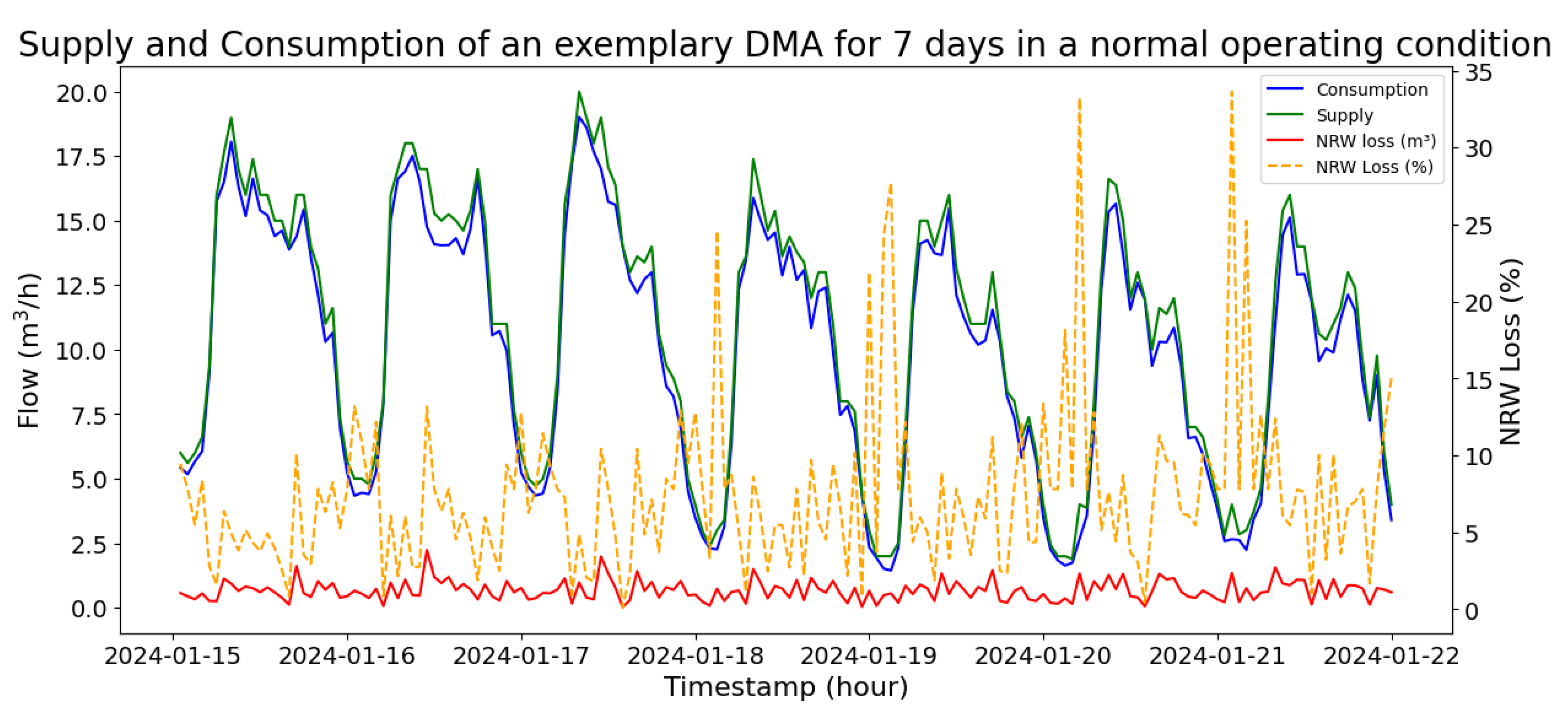
Figure 2.
Core principle of the proposed leak detection framework: For a DMA d, observed normalized consumption is fed to the trained regression model to predict the normalized supply . The predicted supply is compared with the observed normalized supply through the anomaly scoring logic to produce an anomaly score .
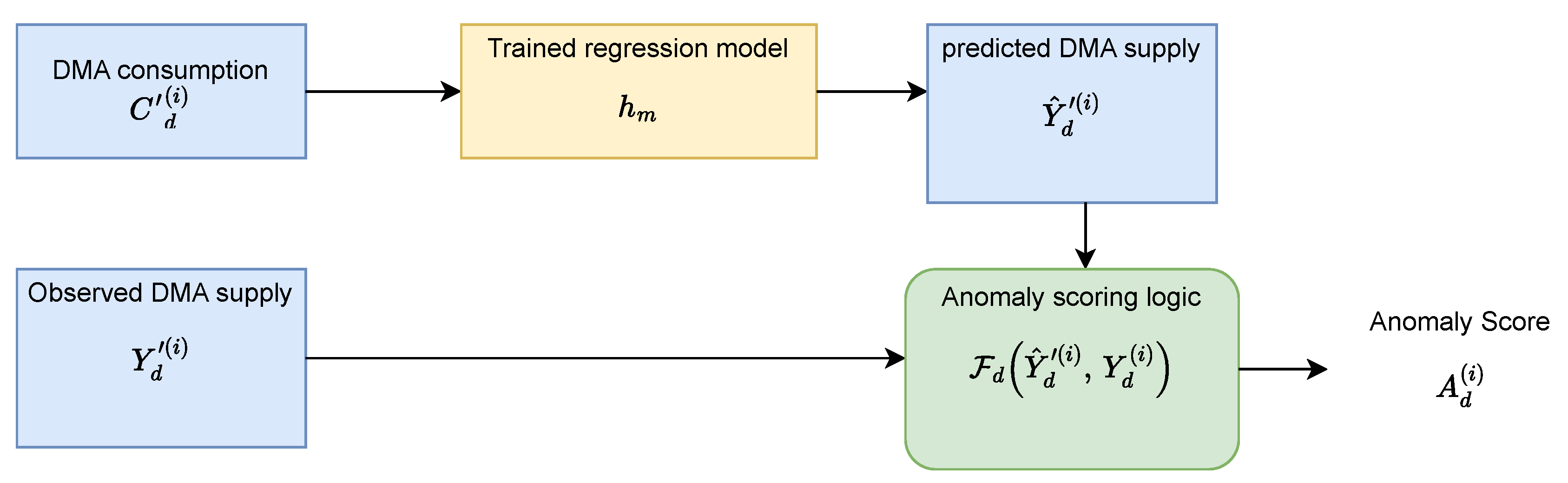
Figure 3.
Method Overview: proposed Ensemble ML Regressor-based framework for leak detection. The system comprises two stages: Offline Consumption-Supply Modeling, where historical data are preprocessed, leak-corrected, and used to train regression models that learn the consumption-supply relationship. Model evaluation yields Metric-Model-DMA (MMD) thresholds for acceptable statistical deviations and Regression Model Opinion (RMO)-weights reflecting model-specific reliability per DMA. In the Online Leak Detection stage, incoming data are transformed using the offline artifacts, and trained models generate predicted supply values. Statistical comparisons between predicted and observed supply are fused through metric-level and model-level ensembles – guided by MMD thresholds and RMO weights – to compute an anomaly score indicating potential leaks.
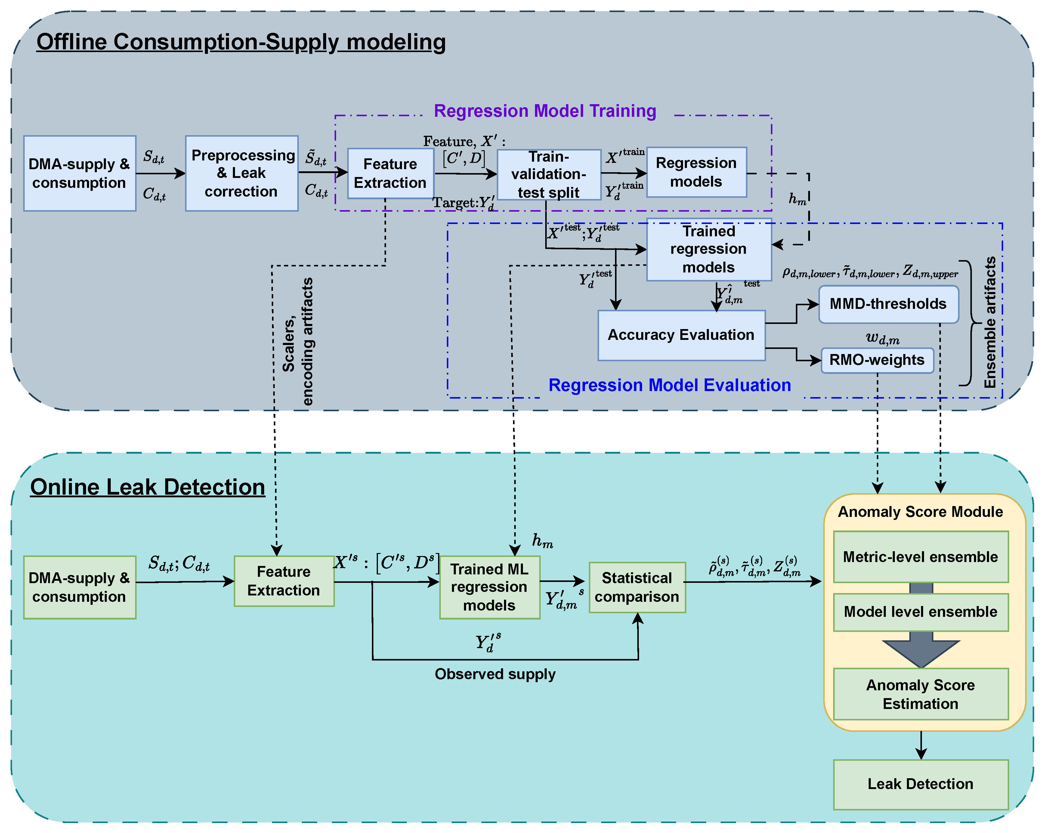
Figure 4.
Calculated consumption and Supply for two exemplary DMAs using the mentioned meter-data preprocessing and aggregation principles
Figure 4.
Calculated consumption and Supply for two exemplary DMAs using the mentioned meter-data preprocessing and aggregation principles
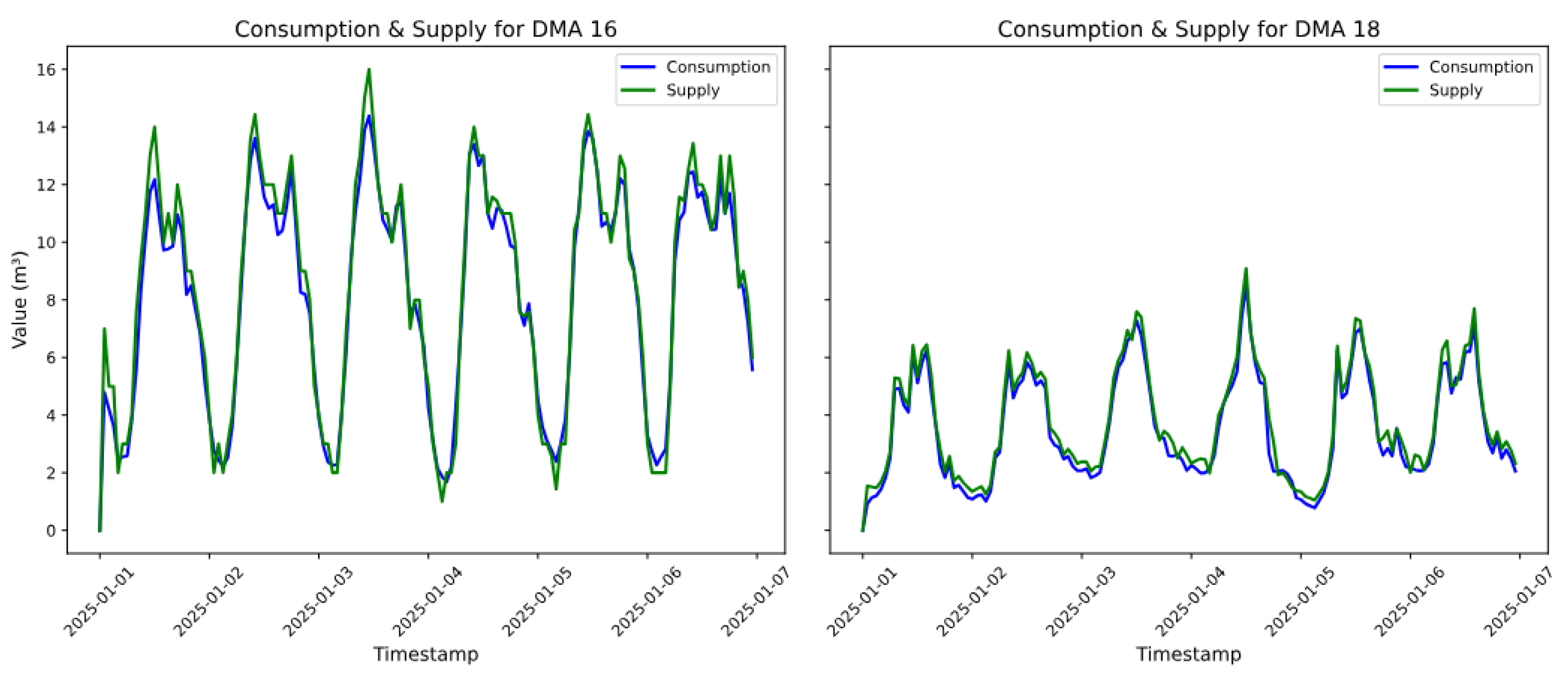
Figure 5.
Before and after correcting unreasonable supply for an exemplary DMA, an example of consumption being higher than supply before correction
Figure 5.
Before and after correcting unreasonable supply for an exemplary DMA, an example of consumption being higher than supply before correction
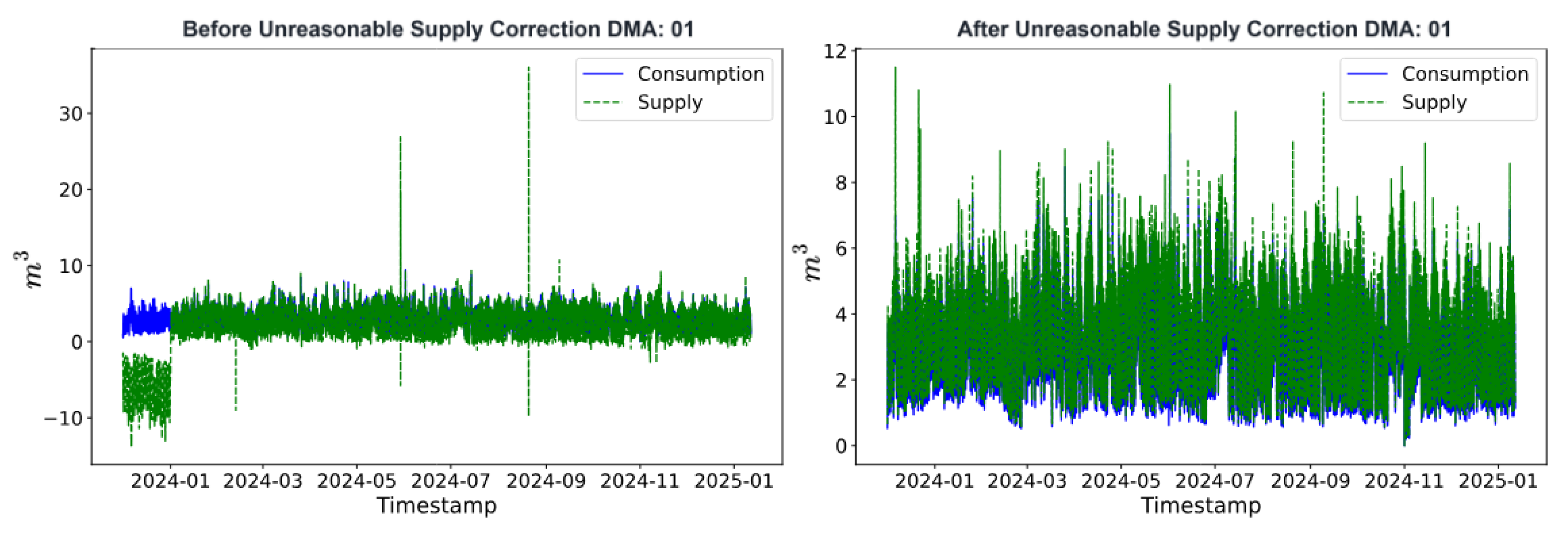
Figure 6.
Before and after correcting unreasonable supply for an exemplary DMA, an example of correcting the effect of leak in the data used for regression model training
Figure 6.
Before and after correcting unreasonable supply for an exemplary DMA, an example of correcting the effect of leak in the data used for regression model training
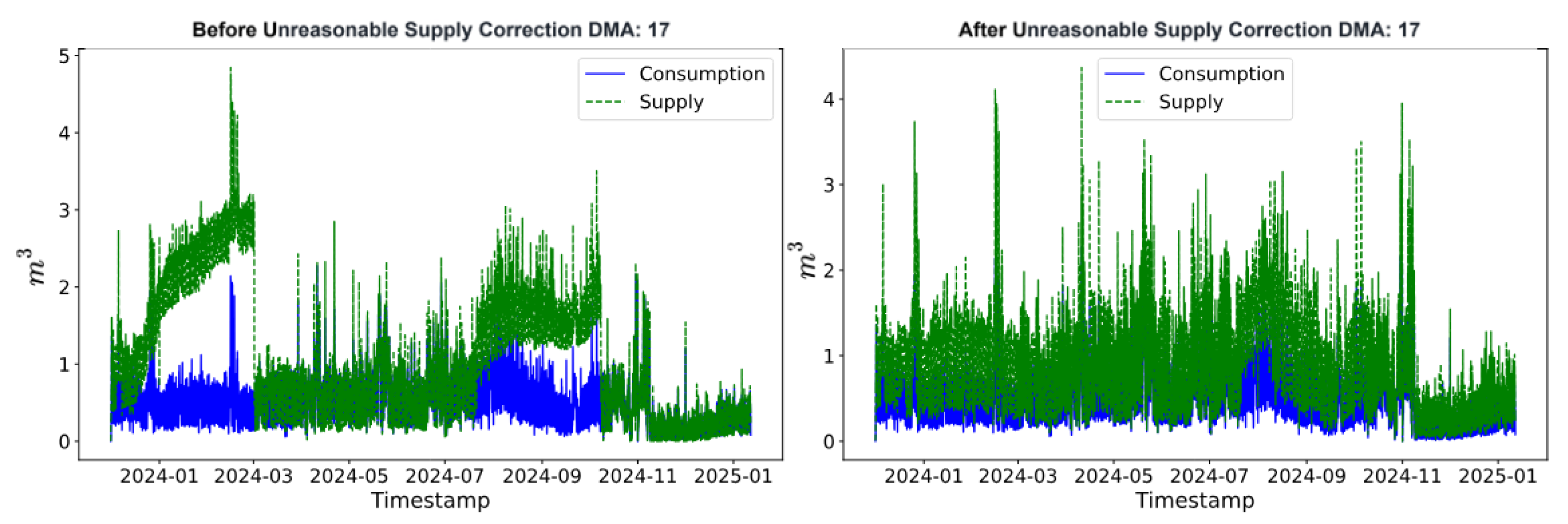
Figure 9.
Exp I: Consumption-Supply Estimation in unified modeling approach
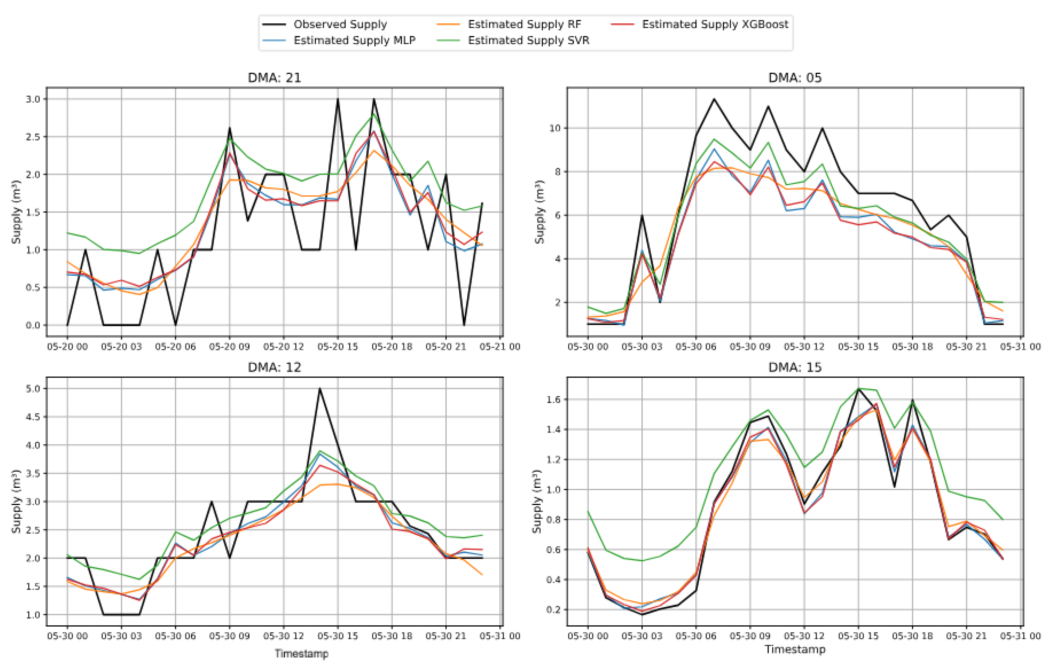
Figure 10.
Exp II: Consumption-Supply Estimation while using DMA-specific models
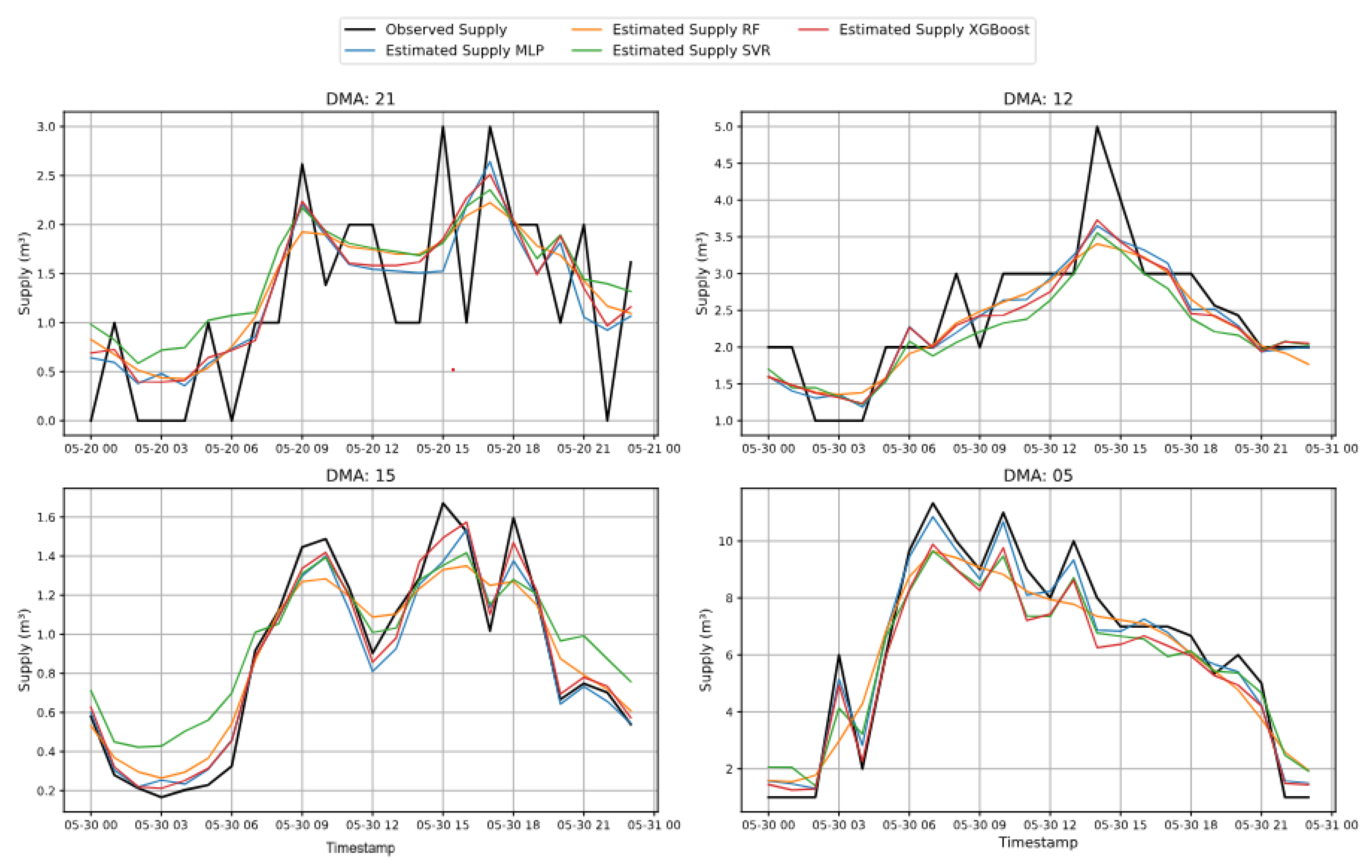
Figure 11.
MAPE and RMSE across different ML algorithms
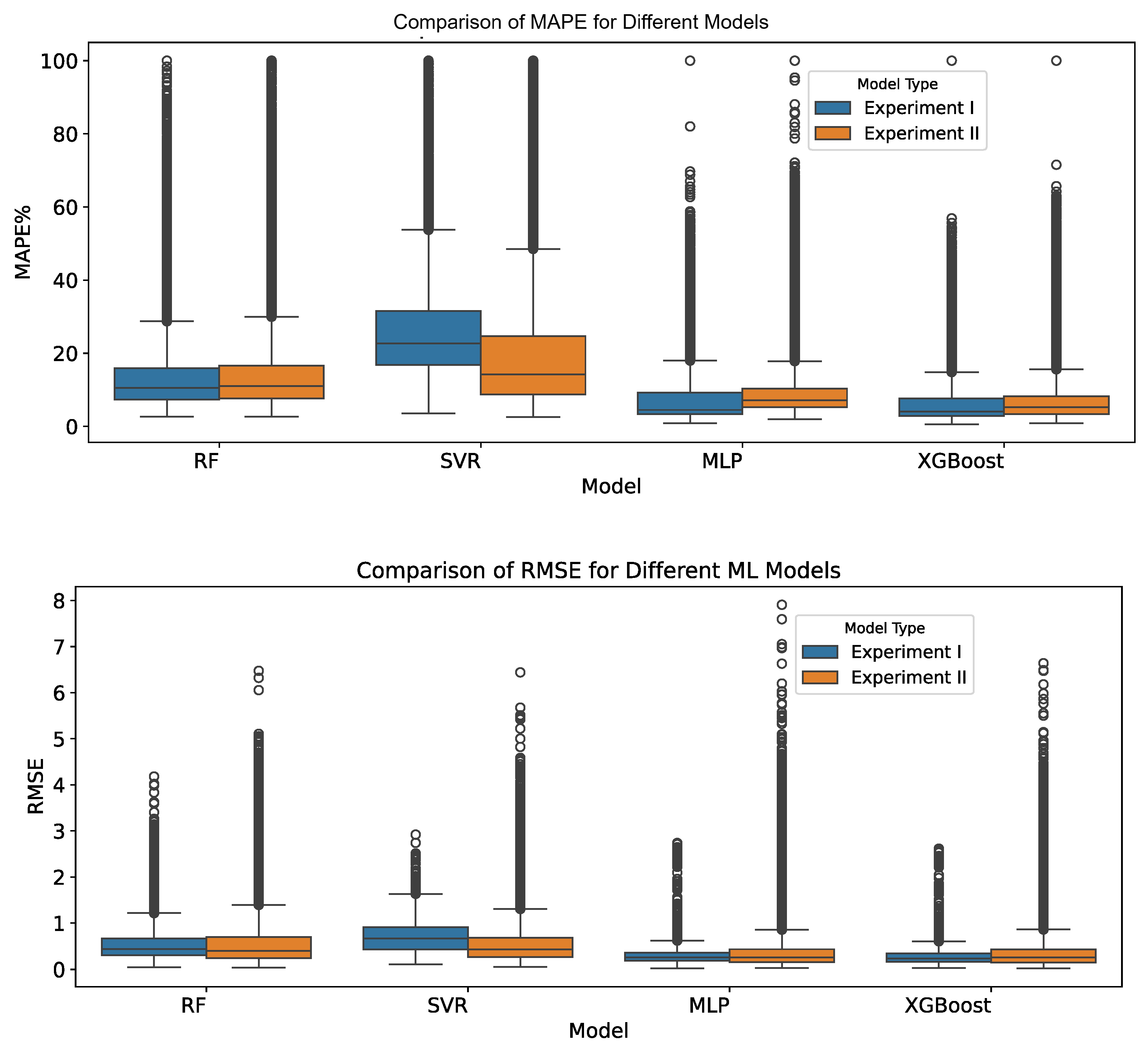
Figure 12.
Simulated leak scenario over a 24-hour window
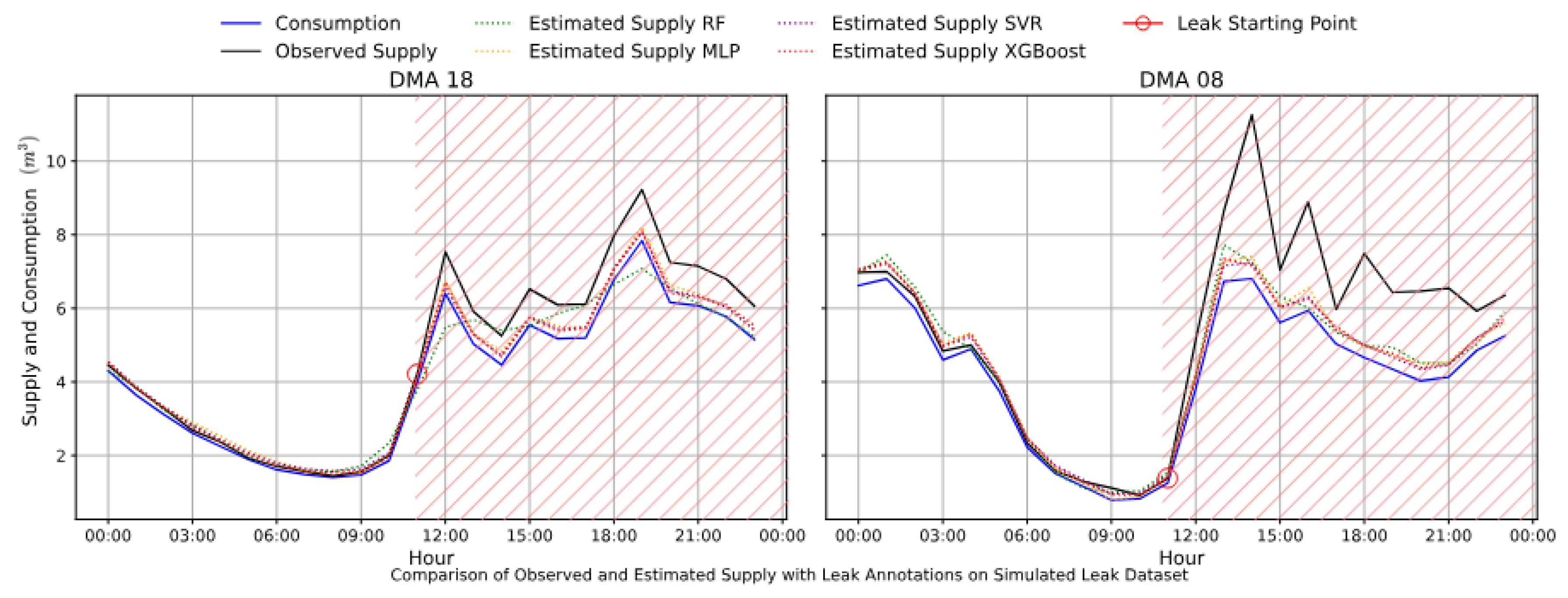
Figure 13.
Real leak scenario over a 24-hour window
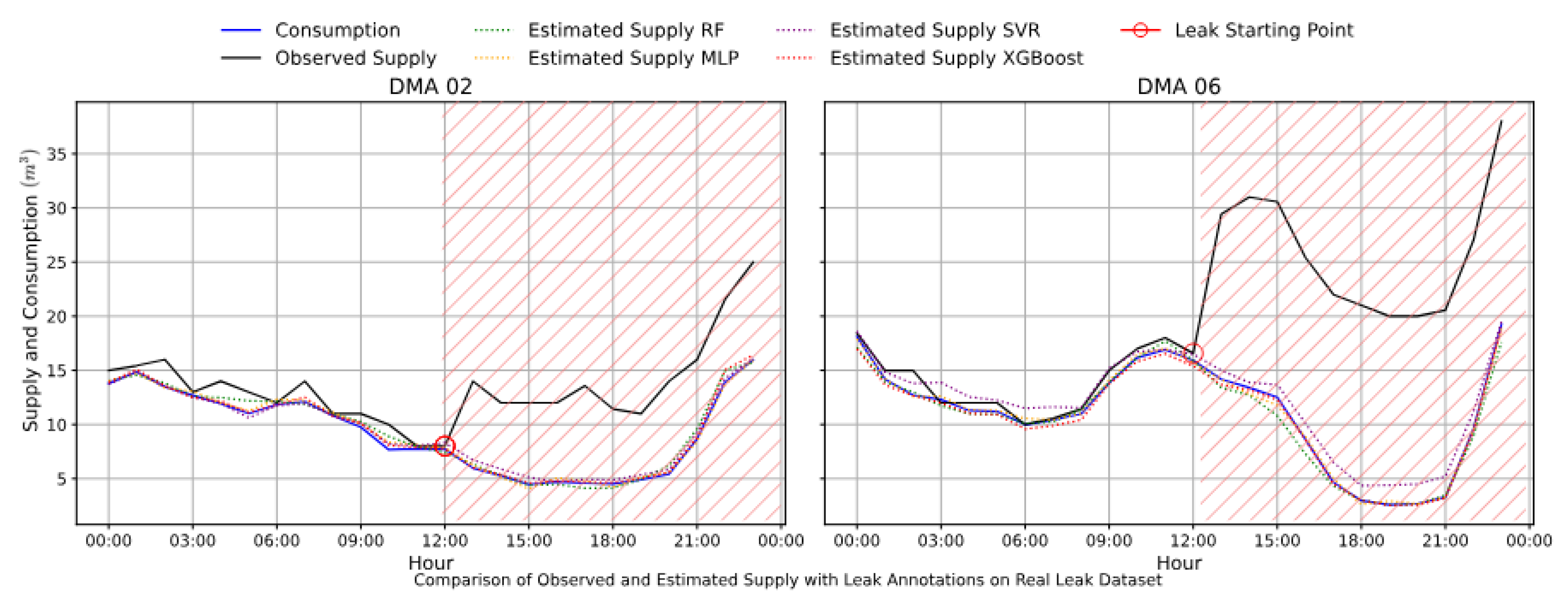
Figure 14.
Exp III: MV Performance on Simulated Leaks (Confusion Matrices)
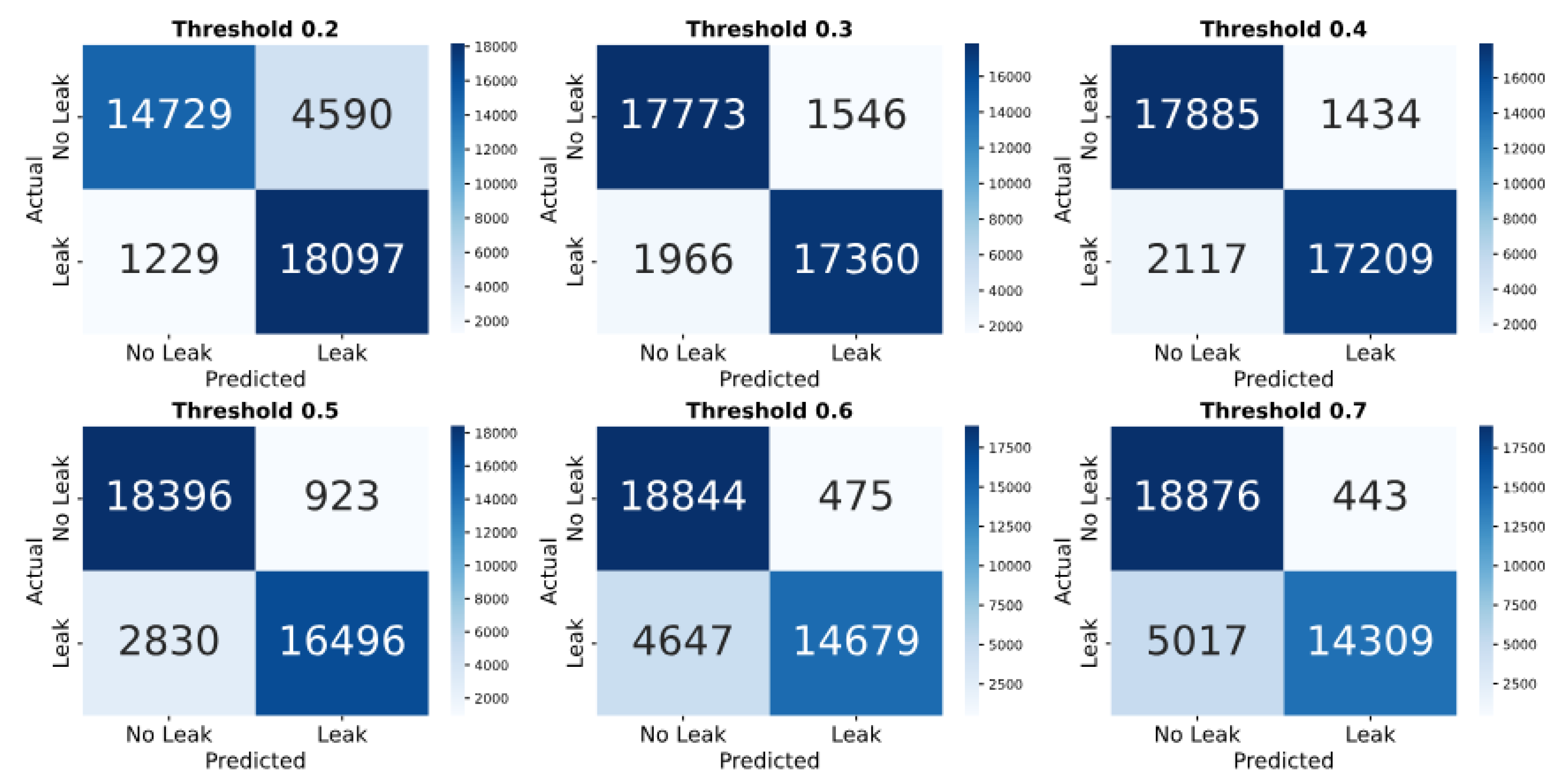
Figure 15.
Exp III: MV Performance on Real Leaks (Confusion Matrices)
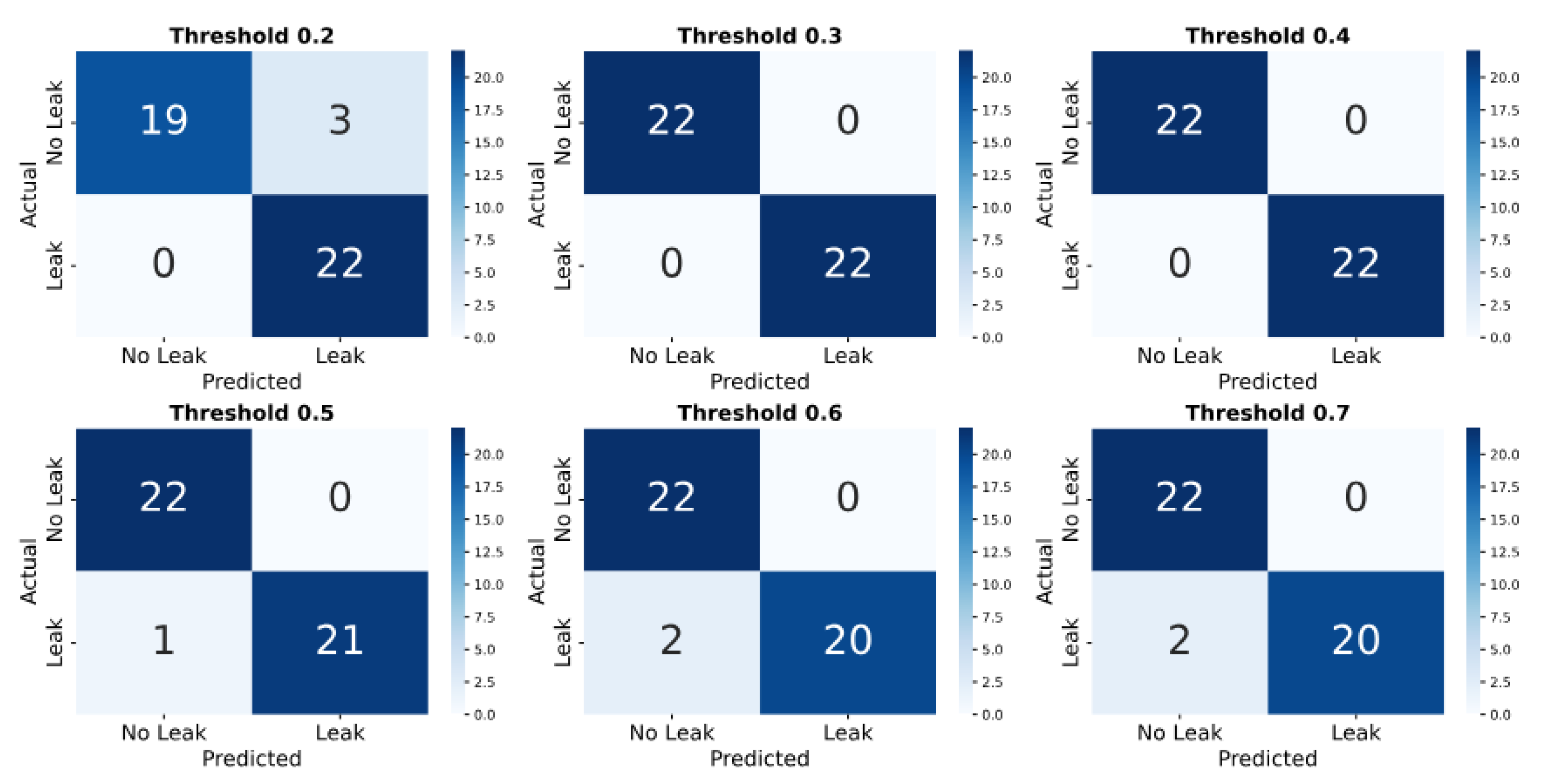
Figure 16.
Exp III: MV Performance Evaluation via ROC Curves (Simulated Leaks)
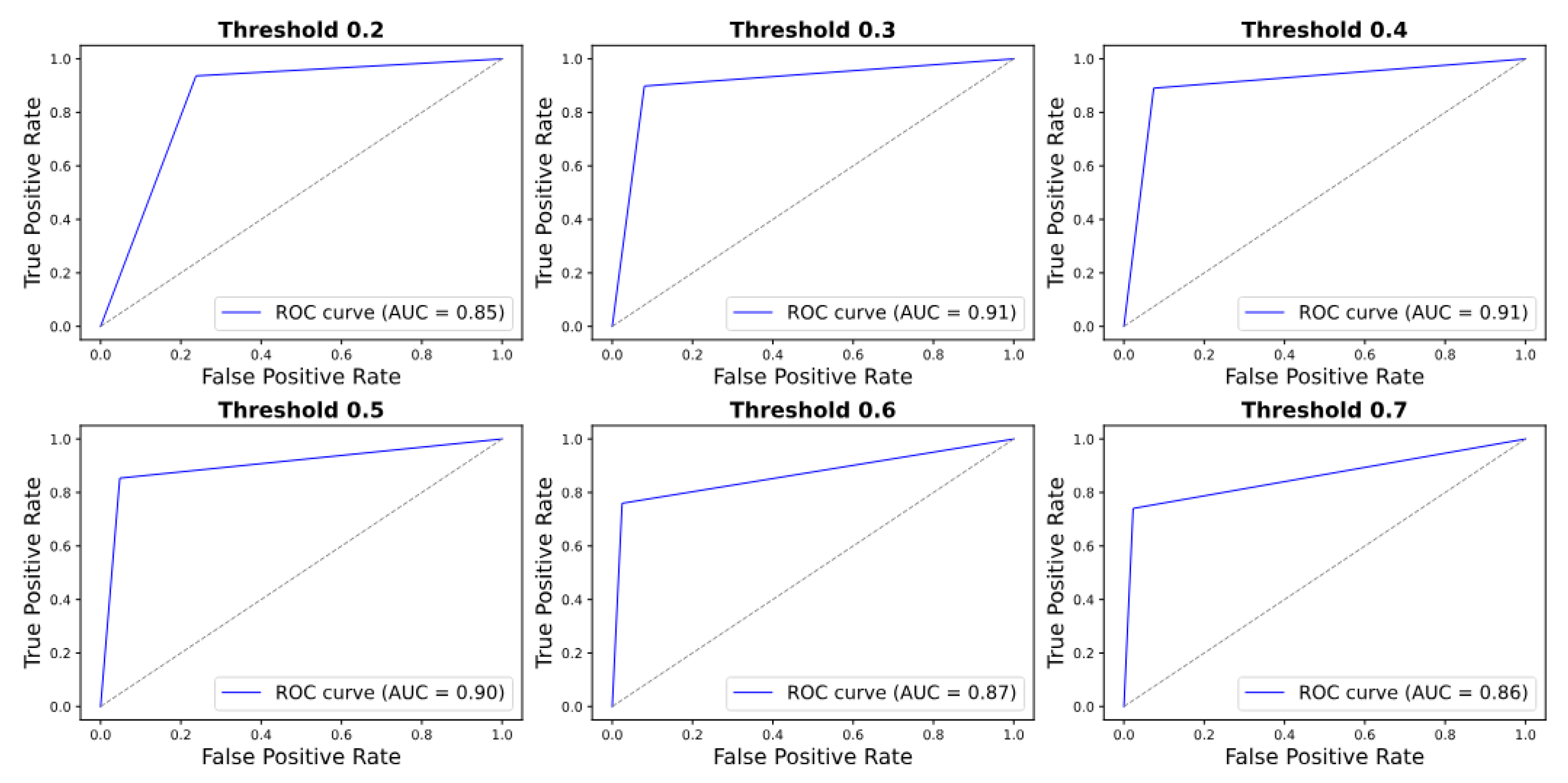
Figure 17.
Exp III: MV Performance Evaluation via ROC Curves (Real Leaks)
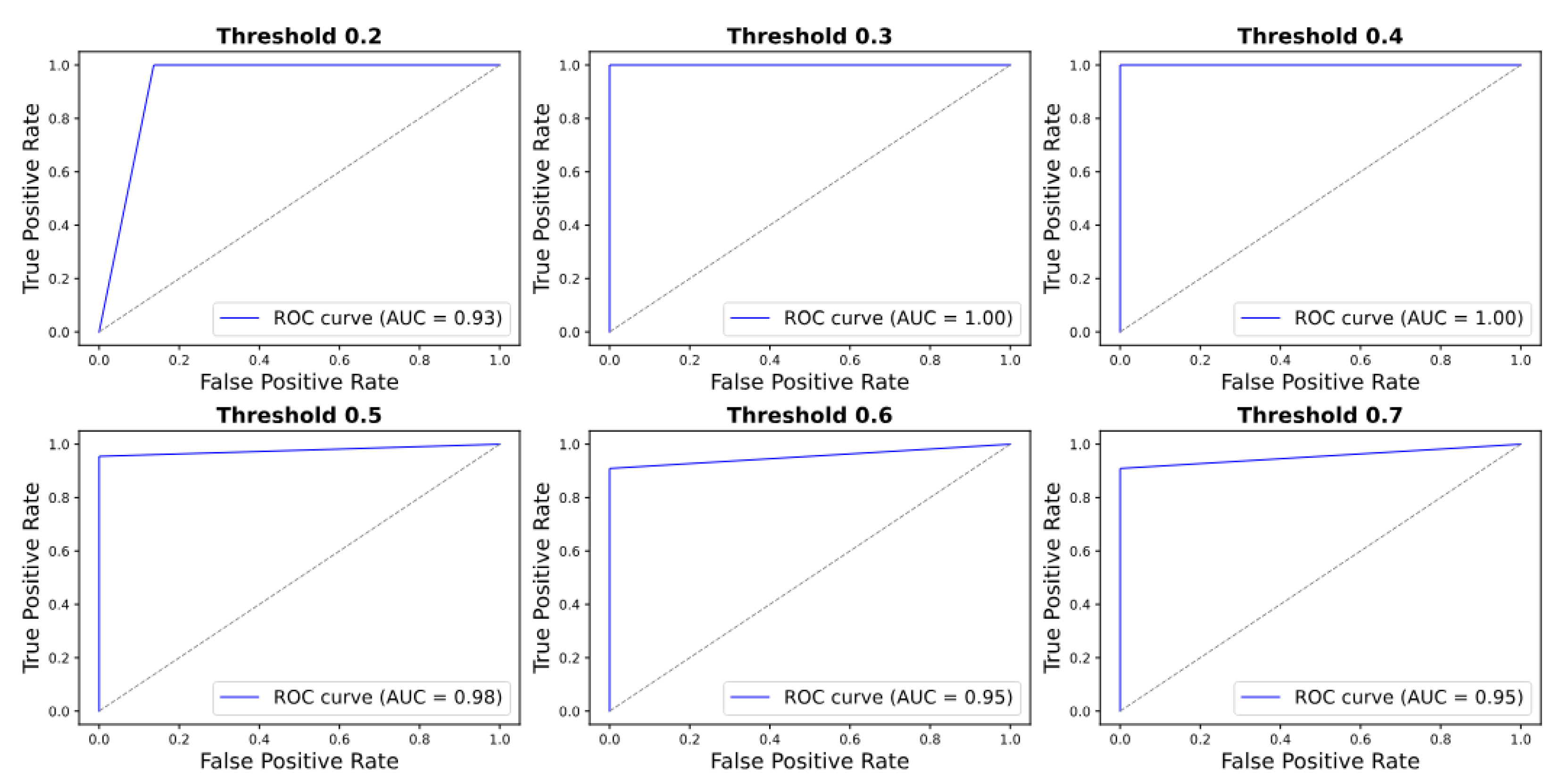
Figure 18.
Exp IV: PS Performance on Simulated Leaks
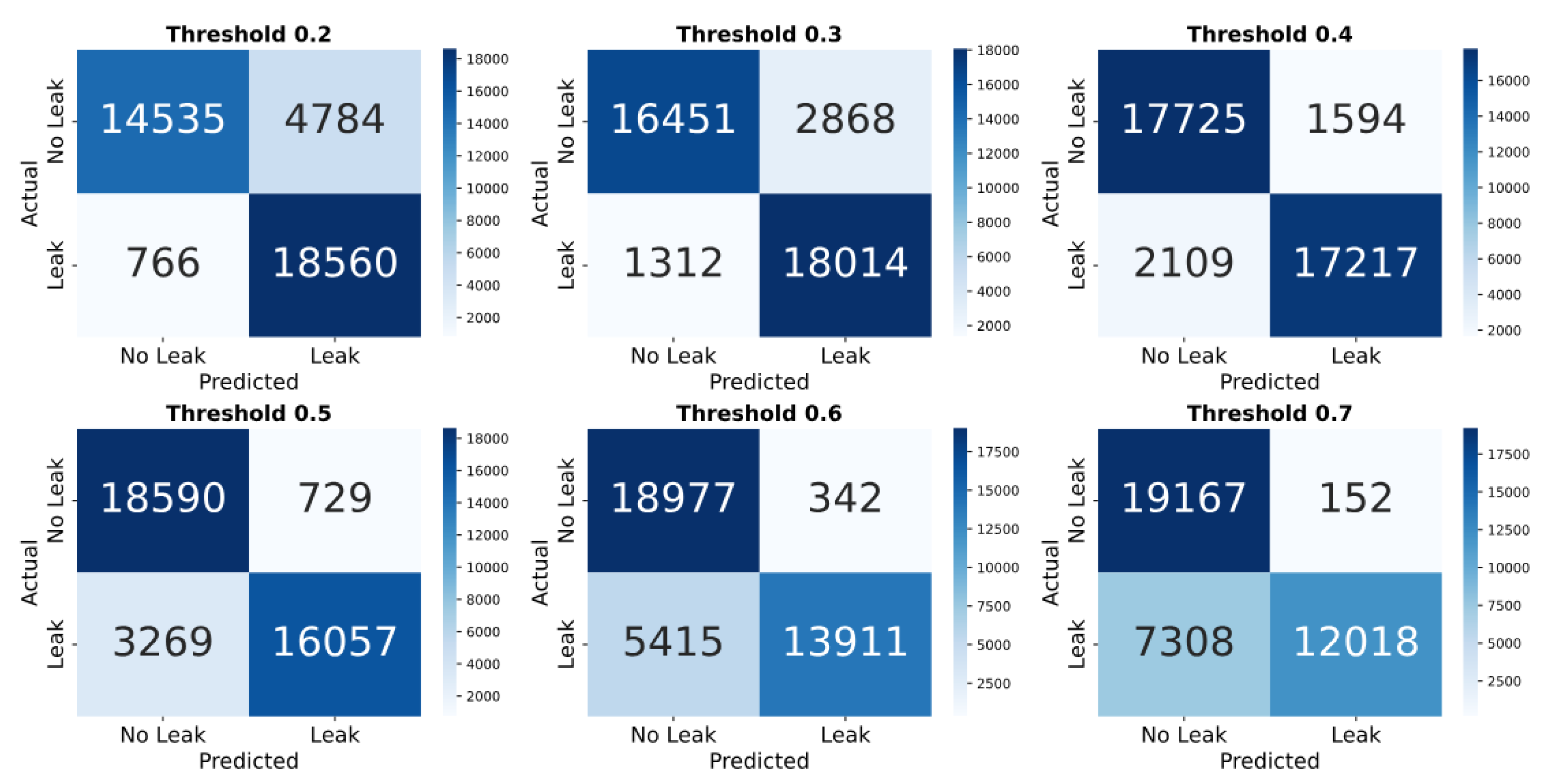
Figure 19.
Exp IV: PS Performance on Real Leaks
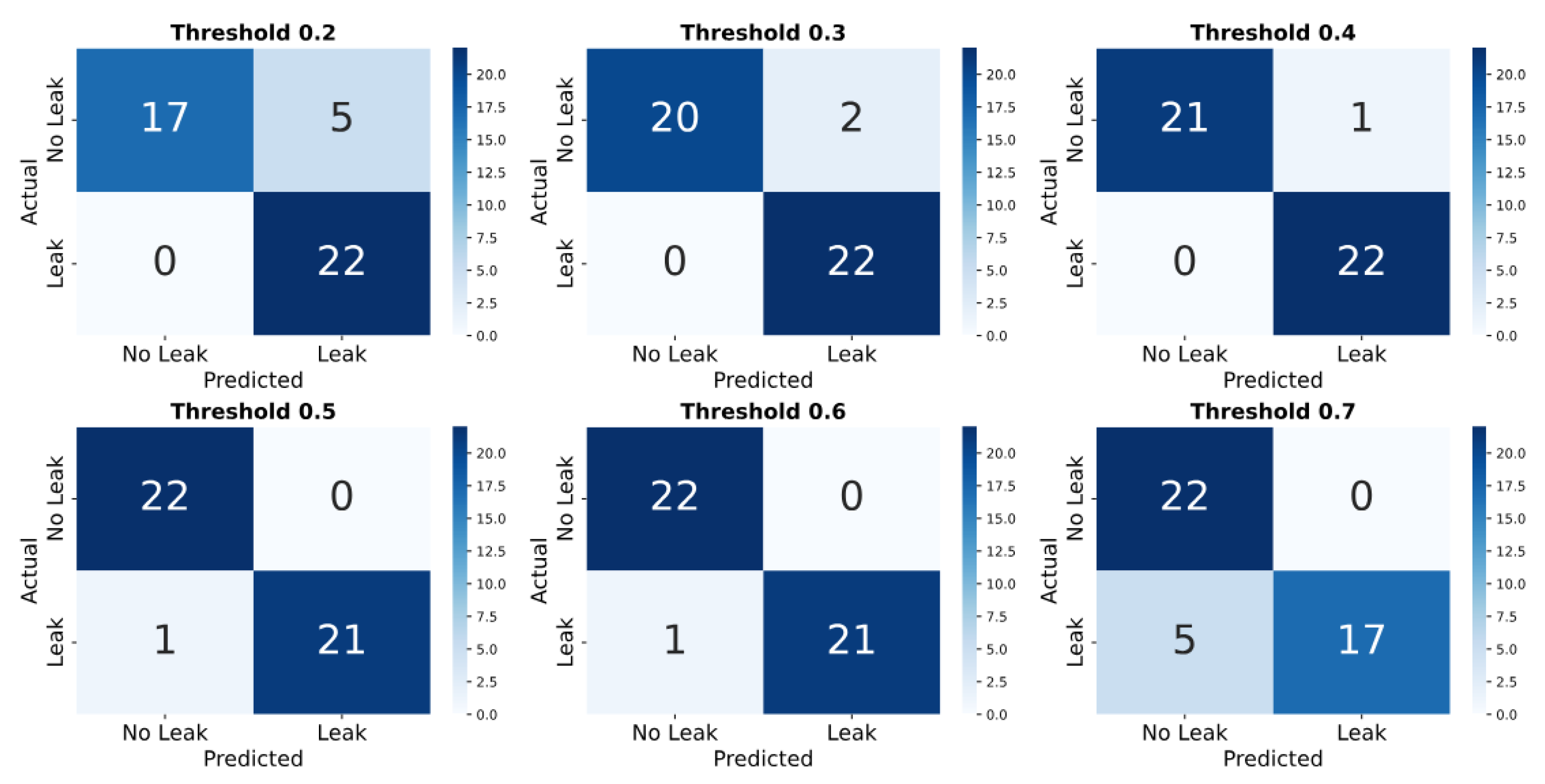
Figure 22.
Leak detection accuracies by using predicted supply from individual regression model: Leak detection accuracy across various leak categories (Left) and Leak detection accuracy across different DMAs (Right), by utilizing individual regression model predicted supply data; Analysis carried out using Simulated-leka dataset)
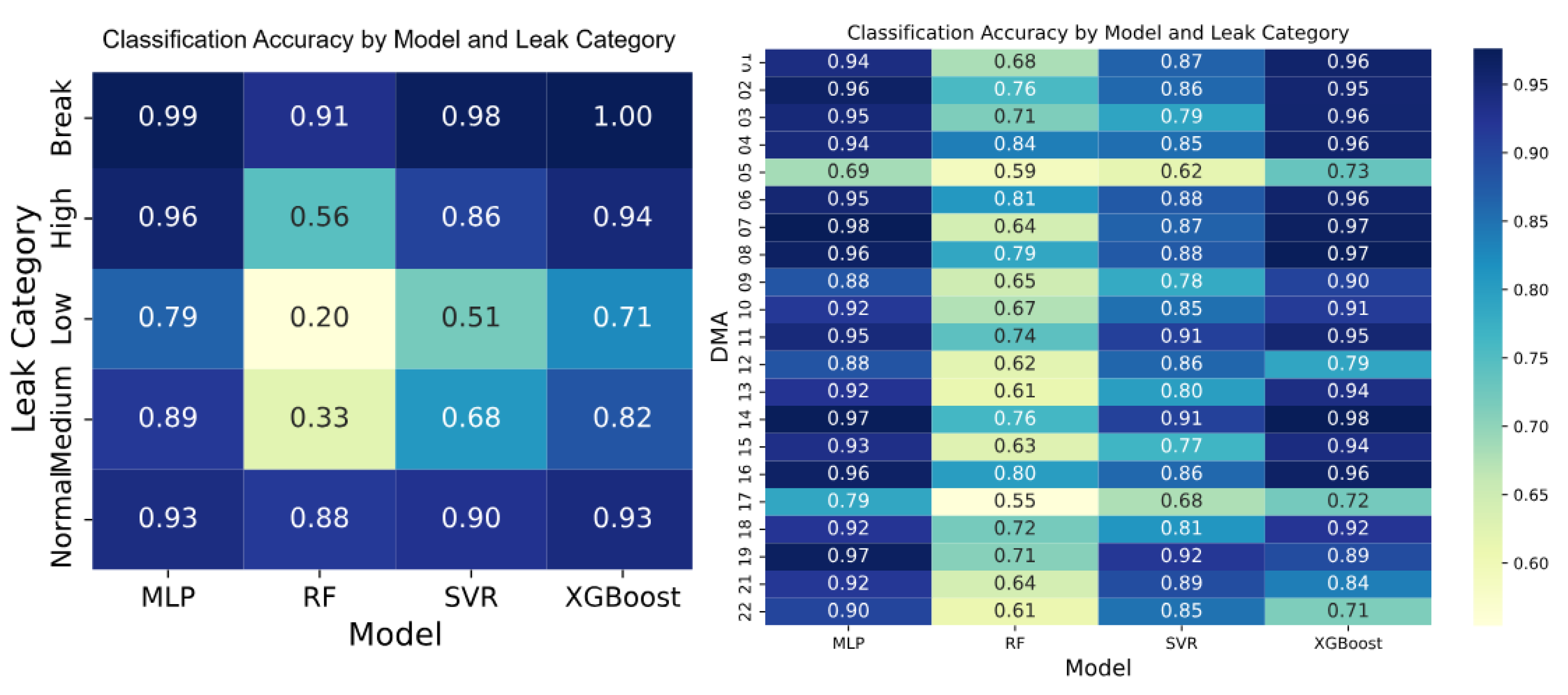
Figure 23.
Ensemble Model Performance by Threshold and Leak Type (Simulated Data)
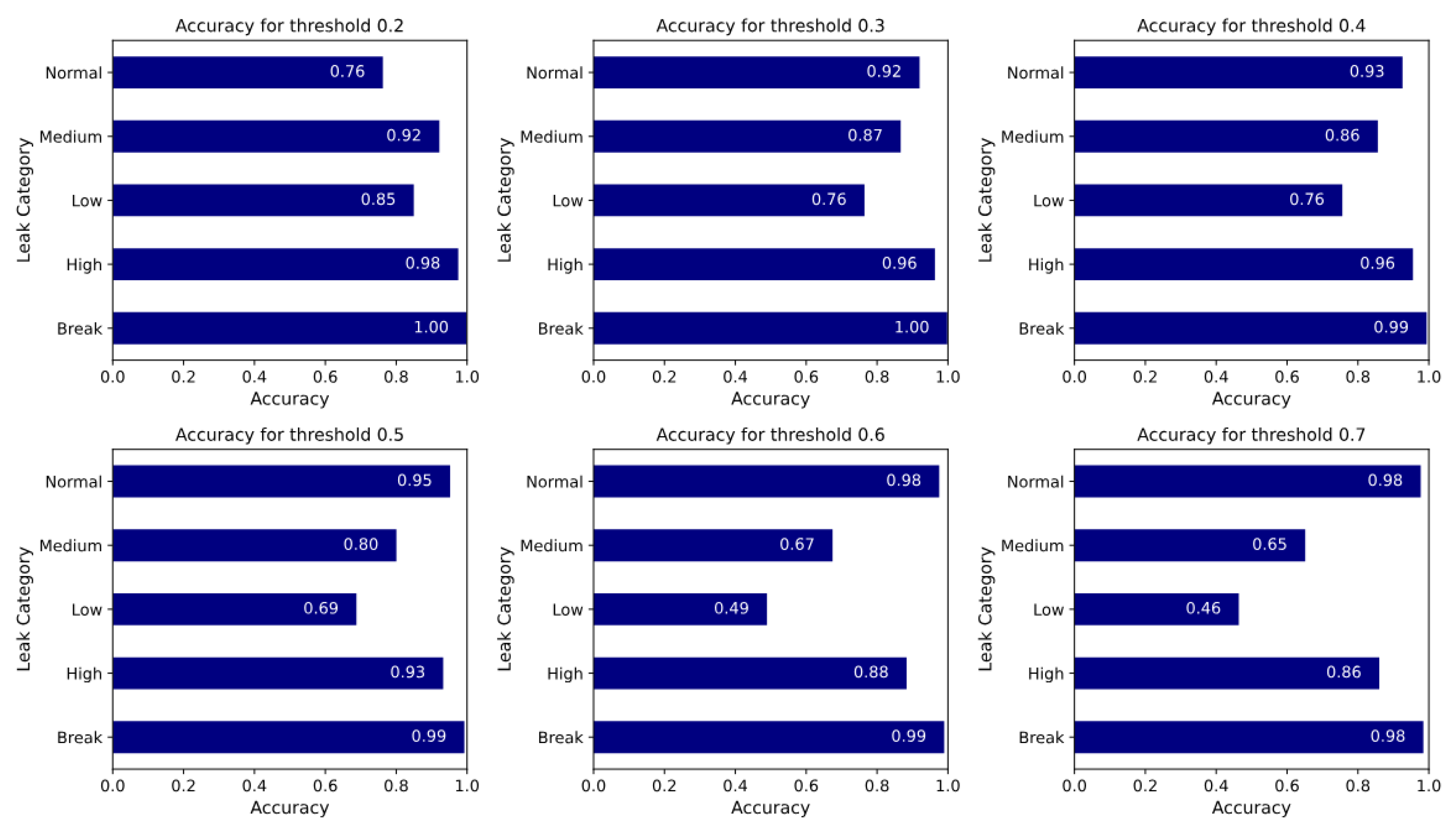
Table 1.
Leak severities based on NRW-loss%
| Leak-severity | Loss Range (%) |
|---|---|
| No-leak | 0–5 |
| Low | 5–8 |
| Medium | 9 |
| High | 15 |
| Break | >15 |
Table 2.
Hyperparameters for Regression Models
| Algorithm | Hyperparameters |
|---|---|
| XGBoost | n_estimators=500, learning_rate=0.05, max_depth=10, |
| subsample=0.8, colsample_bytree=1.0, lambda=10, | |
| alpha=0, min_child_weight=1, gamma=0 | |
| MLP | hidden_layer_sizes=[100, 100], max_iter=200, solver=adam, |
| learning_rate_init=0.001, alpha=0.001, activation=relu | |
| Random Forest | n_estimators=300, max_depth=None, min_samples_split=10, |
| min_samples_leaf=2, max_features=sqrt, bootstrap=True | |
| SVR | C=1.0, epsilon=0.1, kernel=rbf, degree=3, |
| gamma=scale, shrinking=True |
Table 3.
MAPE% and RMSE (mean ± std) for models in Exp I and II
| Model | MAPE% (Mean ± Std Dev) | RMSE (Mean ± Std Dev) | ||
|---|---|---|---|---|
| 2-5 | Experiment I | Experiment II | Experiment I | Experiment II |
| XGBoost | 6.25 ± 5.08 | 6.54 ± 5.22 | 0.27 ± 0.10 | 0.27 ± 0.11 |
| MLP | 7.52 ± 5.47 | 7.87 ± 5.26 | 0.29 ± 0.10 | 0.30 ± 0.10 |
| SVR | 27.79 ± 10.74 | 7.14 ± 5.35 | 0.72 ± 0.09 | 0.29 ± 0.11 |
| RF | 13.66 ± 7.48 | 13.70 ± 7.28 | 0.55 ± 0.20 | 0.56 ± 0.20 |
Table 4.
Exp III: MV Classification Report (Simulated Leaks)
| Threshold | Class | Precision | Recall | F1-score | Accuracy | Support |
|---|---|---|---|---|---|---|
| 0.2 | No Leak | 0.92 | 0.76 | 0.84 | 0.85 | 19319 |
| Leak | 0.80 | 0.94 | 0.86 | 19326 | ||
| 0.3 | No Leak | 0.90 | 0.92 | 0.91 | 0.91 | 19319 |
| Leak | 0.92 | 0.90 | 0.91 | 19326 | ||
| 0.4 | No Leak | 0.89 | 0.93 | 0.91 | 0.91 | 19319 |
| Leak | 0.92 | 0.89 | 0.91 | 19326 | ||
| 0.5 | No Leak | 0.87 | 0.95 | 0.91 | 0.90 | 19319 |
| Leak | 0.95 | 0.85 | 0.90 | 19326 | ||
| 0.6 | No Leak | 0.8 | 0.98 | 0.88 | 0.87 | 19319 |
| Leak | 0.97 | 0.76 | 0.85 | 19326 | ||
| 0.7 | No Leak | 0.79 | 0.98 | 0.87 | 0.86 | 19319 |
| Leak | 0.97 | 0.74 | 0.84 | 19326 |
Table 5.
Exp III: MV Classification Report (Real Leaks)
| Threshold | Class | Precision | Recall | F1-score | Accuracy | Support |
|---|---|---|---|---|---|---|
| 0.2 | No Leak | 1.00 | 0.86 | 0.93 | 0.93 | 22 |
| Leak | 0.88 | 1.00 | 0.94 | 22 | ||
| 0.3 | No Leak | 1.00 | 1.00 | 1.00 | 1.00 | 22 |
| Leak | 1.00 | 1.00 | 1.00 | 22 | ||
| 0.4 | No Leak | 1.00 | 1.00 | 1.00 | 1.00 | 22 |
| Leak | 1.00 | 1.00 | 1.00 | 22 | ||
| 0.5 | No Leak | 0.96 | 1.00 | 0.98 | 0.98 | 22 |
| Leak | 1.00 | 0.95 | 0.98 | 22 | ||
| 0.6 | No Leak | 0.92 | 1.00 | 0.96 | 0.95 | 22 |
| Leak | 1.00 | 0.91 | 0.95 | 22 | ||
| 0.7 | No Leak | 0.92 | 1.00 | 0.96 | 0.95 | 22 |
| Leak | 1.00 | 0.91 | 0.95 | 22 |
Disclaimer/Publisher’s Note: The statements, opinions and data contained in all publications are solely those of the individual author(s) and contributor(s) and not of MDPI and/or the editor(s). MDPI and/or the editor(s) disclaim responsibility for any injury to people or property resulting from any ideas, methods, instructions or products referred to in the content. |
© 2026 by the authors. Licensee MDPI, Basel, Switzerland. This article is an open access article distributed under the terms and conditions of the Creative Commons Attribution (CC BY) license (http://creativecommons.org/licenses/by/4.0/).
Copyright: This open access article is published under a Creative Commons CC BY 4.0 license, which permit the free download, distribution, and reuse, provided that the author and preprint are cited in any reuse.


