
Submitted:
20 January 2026
Posted:
20 January 2026
You are already at the latest version
Abstract
Intrusion Detection Systems (IDSs) have evolved to safeguard networks and systems from cyber attacks. Anomaly-based Intrusion Detection Systems (A-IDS) have been commonly employed to detect known and unknown anomalies. However, conventional anomaly detection approaches encounter substantial challenges when dealing with complex, large-scale, and heterogeneous data sources. These challenges include high False Positive Rates (FPRs), imbalanced data behavior, complex data handling, resource constraints, limited interpretability, and difficulties with encrypted networks.
This survey reviews Graph-based Anomaly Detection (GBAD) approaches, highlighting their ability to address these challenges by utilizing the inherent structure of graphs to capture and analyze network connectivity patterns. GBAD approaches offer flexibility for handling diverse data types, scalability to analyze large datasets, robustness detection capabilities, and enhanced interpretability through visualizations. We present a phased graph-based anomaly detection methodology for intrusion detection. This includes phases of data capturing, graph construction, graph pre-processing, anomaly detection, and post-detection analysis. Furthermore, we examine the evaluation methods and datasets employed in GBAD research and provide an analysis of the types of attacks identified by these methods.
Lastly, we outline the key challenges and future directions that require significant research efforts in this area and offer some recommendations to address them.
Keywords:
graph anomaly detection
; network intrusion detection
; attack detection
1. Introduction
Cyber threats have increased in numerous sectors in recent years, and these threats have significantly impacted critical system components, often resulting in substantial recovery costs. For example, DP World, a port operator in Australia, recently reported an IT breach that impacted critical systems to coordinate shipping activities [1]. Several cyber incidents caused by sophisticated anomalous behaviors cost Optus $140 million and $35 million for Medibank to cover data breaches [2]. The complexity and heterogeneity of modern networks further complicate the detection of these threats, making cybersecurity efforts even more challenging [3]. The need for anomaly detection systems has increased significantly in detecting and mitigating cyber intrusions. Recently, according to the Global Market Report on Anomaly Detection [4], the global market size for anomaly detection was valued at USD 2.40 billion in 2022 and is expected to reach USD 8.85 billion by 2032, with an anticipated revenue CAGR of 15.6% over the forecast period. The increasing prevalence of sophisticated cyberattacks has made anomaly detection a crucial component of organizational cybersecurity, requiring a variety of detection methods, including graph-based techniques, to identify and mitigate potential threats.
Intrusion Detection System (IDS) monitors and analyzes the system activities to detect unauthorized access and attempts to compromise the confidentiality, integrity, or availability of resources [5]. Intrusion detection techniques are categorized into Misuse Detection, which identifies known attacks using signatures, and Anomaly Detection, which predicts new and unknown threats [6].
Anomaly-based intrusion detection focuses on uncovering security breaches, unauthorized access attempts, or malicious activities jeopardizing system security, considering behavior deviations. For instance, anomalies detected within network traffic and system logs are utilized to trigger outliers as malicious behaviors or signs of a cyber attack. Cyber attackers obscure their actions in complex networks by exploiting complex interconnections and vast data volumes to blend in with normal traffic patterns, posing challenges for traditional security measures to detect anomalous activities [7].
Further, conventional anomaly-based IDSs encounter several challenges, including high False Positive Rates (FPRs) [8,9], reliance on large labeled datasets [10,11], and difficulty in capturing evolving or complex behaviors [11]. The specification or rule-based anomaly detection methods, depending on domain knowledge [11], make it difficult to adapt to new or evolving threats. Additionally, deep learning methods, though powerful, demand substantial computational resources and lack transparency, making it complex for security teams to interpret and respond to alerts effectively [12]. The complexity of modern threats, such as APTs, and the rise of encrypted networks underscore the need for more adaptable and interpretable anomaly detection systems [13,14].
Graph-based anomaly detection (GBAD) addresses current challenges by leveraging relational analysis and intelligent detection methods to reduce false positives [8], scalable graph-based algorithms for complex models [15], and visualizations for interpretability [16]. Further, it balances behaviors through graph-based sampling and weighting, detects evasion techniques using pattern recognition, adapts to concept drift through incremental updates [17], and integrates with security controls via graph-based models. By utilizing graph structures, it captures complex relationships and patterns, improving detection accuracy and efficiency while reducing false alarms and enhancing explainability [18]. In addition, by incorporating techniques like novelty detection and semi-supervised learning, graph-based approaches reduce reliance on labeled data and handle the data imbalance by focusing on modeling normal data when there is insufficient abnormal data [19,20]. Given these advantages, it is certainly worth further investigation into graph-based anomaly detection as a promising approach for intrusion detection.
Existing reviews: Existing surveys on anomaly detection and intrusion detection span a range of domains, from conventional methods to graph-based approaches. In recent years, numerous surveys have explored various aspects of anomaly detection in network infrastructures. For instance, the surveys of Eltanbouly et al. [28] and Kwon et al. [29] centered on machine learning and deep learning-based methods for network traffic anomaly detection. Moustafa et al. [30] examined Decision Engine (DE) approaches, including ensemble and deep learning techniques for network anomaly detection. Recent attention has also shifted toward graph-based techniques for anomaly detection beginning with the publication of Akoglu et al. [18] offered an extensive overview and categorization of conventional graph-based anomaly detection approaches. Since then, several GBAD-focused surveys have emerged, though they tend to be narrow in scope, concentrating on specific applications, graph types, or particular methods (e.g., GNN-based models). For instance, recent GBAD-focused surveys have targeted a single application area, such as botnet detection [25], intrusion detection [26,27], fraud detection [21], and anomaly detection in distributed systems [24].
Others have focused on specific graph types, such as provenance graphs [22], or a specific GBAD approach, such as GNN-based anomaly detection [23,26,27]. Among the GNN-based surveys, the works by Zhong et al . [27] and Bilot et al. [26] align closely with our work, however their surveys are limited to GNN-based methods and categorize techniques based on graph construction, network design, deployment types, and anomaly levels. To the best of our knowledge, no existing survey has comprehensively examined the broader spectrum of GBAD methods beyond GNNs, specifically in the context of intrusion detection. Therefore, our focus is on GBAD approaches specifically applied to intrusion detection, as illustrated in the Figure 1, and on identifying the complete workflow involved in the GBAD-based intrusion detection process.
Most notably, our paper offers a comprehensive analysis of the entire GBAD workflow from data capture to post-detection analysis. This systematic examination of each phase in the GBAD process provides a broader perspective and a structured framework for understanding how each stage contributes to the overall intrusion detection process. We introduce a concept of graph classification based on the types of data captured (e.g., network traffic, system logs, CAN data) and categorize GBAD methods into GRL-based approaches (two-stage) and end-to-end graph-based approaches. We investigated various techniques within these categories, including graph clustering, graph analysis, and graph scoring methods, emphasizing their application to intrusion detection. The novelty of our research lies in conducting a comprehensive investigation into a phased, graph-based anomaly detection framework for intrusion detection. We provide an extensive set of methods, techniques, and algorithms applied at each stage of the detection process in this framework, thereby enabling the implementation of more accurate detection techniques by selecting the most suitable method for each stage. The summary in Table 1 offers an overview of existing research in anomaly detection using graph-related techniques and further highlights the contributions of our survey.
Our Contributions: This survey advances the understanding of GBAD for intrusion detection through four key contributions: (1) It presents the first comprehensive investigation of the complete GBAD workflow, from data capture to post-detection analysis, offering a systematic analysis of techniques at each phase. (2) The survey introduces a novel categorization framework, distinguishing between two-stage and end-to-end GBAD approaches, providing an in-depth analysis and structured comparison of their methodologies. (3) It delivers a thorough evaluation of assessment methodologies in GBAD research, examining both the benchmark datasets and evaluation metrics used to validate detection effectiveness. (4) Finally, it identifies critical challenges and emerging opportunities in GBAD implementation, offering concrete recommendations for future research directions in improving detection accuracy, scalability, and real-time performance for intrusion detection.
Papers included in this survey: In this survey, we utilized Google Scholar, ACM Digital Library, Springer, Elsevier, and IEEE Explorer to identify primary studies from the last five years, from 2019 to 2025. The search query used to pinpoint specific technical papers relevant to the research question was: ("graph") AND ("anomaly" OR "outlier") AND ("attack detection" OR "intrusion detection"). This query was developed through a process of trial and error. We then refined our selection to include only those papers that applied graph-based methods throughout the anomaly detection process. Additionally, we prioritized papers based on their citation counts and published venues. Specifically, we selected papers with high citation counts or those published in high-impact conferences and journals, including top-tier security conferences (e.g., IEEE S&P, NDSS, ACM CCS, USENIX Security) and Q1/Q2-ranked journals (e.g., IEEE Transactions on Information Forensics and Security, Elsevier Computers & Security). While papers with over 100 citations were preferred due to their demonstrated impact, we also included recent high-quality contributions with fewer citations, identified through a manual snowballing approach. In total, we included 60 technical papers for this survey. Of these, 18 focus on GNN-based anomaly detection methods, while the remaining 42 cover other GBAD approaches such as graph clustering, graph scoring, and graph divergence analysis. To ensure methodological rigor, we adopted the Kitchenham and Charters systematic literature review (SLR) guidelines, widely accepted in computing and engineering research. This framework ensured a structured and reproducible process, including review planning, paper selection using inclusion/exclusion criteria, manual snowballing, data extraction aligned with research questions, and classification based on anomaly detection workflow stages.
The rest of this survey is structured as follows. We provide the background on graph-based anomaly detection within the broader context of anomaly detection in Section 2. Next, we propose a research methodology for categorizing graph-based anomaly detection methods in Section 2.3 and detail the use of graphs and various techniques at each phase of anomaly detection processes. The subsections from 3 to 6 cover these phases in-depth, covering the methods and techniques applied at each stage. The evaluation methods and datasets used for assessment are discussed in Section 6.1 and Section 6.1.1, respectively. Finally, Section 7 discusses the lessons learned and identifies open challenges in graph-based methods and intrusion detection, offering directions for future research.
2. Overview of Graph-based Anomaly Detection for Intrusion Detection
This section defines anomaly detection followed by challenges faced by traditional anomaly detection methods and examine the unique capabilities of graph-based anomaly detection approaches. As a key contribution of this study, we presented a novel GBAD workflow for intrusion detection identified based on insights from the reviewed papers.
2.1. Overview of Anomaly Detection
2.1.1. Definitions of Anomaly Detection
Anomaly detection is a fundamental aspect of data analysis that identifies patterns deviating from expected behavior. While definitions vary across literature, they share common elements. Nassif et al. [31] characterizes anomalies as patterns that diverge from anticipated behavior, while Chalapathy et al. [32] emphasizes the significant deviation from majority patterns. Also known as profile-based detection, this methodology establishes a baseline profile of typical behavior within a dataset or system. In IDSs, this baseline serves as a reference point against which current data is compared to identify potential security threats or malicious activities [33,34].
2.1.2. Definitions of Graph-based Anomaly Detection
Graph-based anomaly detection (GBAD) represents a sophisticated approach to identifying unusual patterns by analyzing the structural relationships within graph databases. This method, formalized by Akoglu et al. [18], excels at detecting rare or significantly different graph objects (nodes, edges, or substructures) by leveraging the inherent interconnections among data elements. As highlighted by Sensarma et al. [35], the increasing ubiquity of graph data has sparked numerous studies exploring its potential in anomaly detection, particularly due to its ability to capture long-range correlations between objects. GBAD methodologies can be classified based on the type of anomalous component (i.e., node, edge, subgraph), graph type (i.e., static, dynamic), method used (i.e., probabilistic/statistical-based, matrix/tensor decomposition-based, and distance/similarity-based methods) and anomaly type (i.e., sparse anomaly, group anomaly, sudden anomaly, gradual anomaly) [36]. The core formulation of the GBAD methods typically begins with a graph defined as where V is the set of nodes, E is the set of edges and Y is the set of labels representing the normal or anomalous states of graph elements (nodes, edges, or the entire graph). The goal of anomaly detection is to learn a mapping function for one of the following tasks: node-level anomaly detection, edge-level anomaly detection or graph-level classification.
The implementation of GBAD follows a structured methodology, comprising graph construction, embedding, and detection phases. Li et al. [37] exemplified this approach through a log anomaly detection system that incorporates five key steps: log parsing, grouping, graph construction, representation learning, and anomaly detection. These phases are elaborated in detail under Section 2.3.
2.2. Anomaly Detection Approaches for Intrusion Detection
An Intrusion Detection System (IDS) serves as an automated defense mechanism that monitors, detects, and analyzes hostile activities within networks or hosts [38]. IDS implementations can be categorized based on two primary aspects: data source and detection strategy. Data source classification distinguishes between host-based IDS (i.e., monitoring internal system activities) and network-based IDS (i.e., analyzing network traffic) [39]. The detection strategy classification separates signature-based from anomaly-based approaches, with Anomaly-based IDS (A-IDS) offering distinct advantages such as unknown attack detection and zero-day threat identification, despite challenges like higher false alarm rates [39]. In this survey, we mainly focus on Anomaly-based IDS (A-IDS).
2.2.1. Conventional Anomaly Detection Approaches:
In cybersecurity, the conventional anomaly detection plays a crucial role in identifying potential attacks [31]. Regarding the scope of this survey paper, anomalies represent abnormal patterns in data sources indicative of cyber attacks. Network anomalies, which can be either malicious (e.g., DoS attacks, port scans) or non-malicious (configuration errors, line interruptions), are classified according to their nature and causal aspects [38]. Nature-based categories encompass three main types [31,40,41]. Point anomalies represent individual deviations, such as User to Root (U2R) and Remote to Local (R2L) attacks, while collective anomalies involve group-based deviations exemplified by DoS attacks. Contextual anomalies complete this classification, representing context-dependent deviations often seen in probe attacks [42].
The causal aspect classification provides another perspective on network anomalies [38,43,44]. Operational anomalies stem from infrastructure-related issues within the network. Flash crowd anomalies occur when resources are overwhelmed by sudden usage spikes. Measurement anomalies arise from inaccuracies in data collection processes. Network attacks, including DoS and DDoS, represent malicious activities deliberately designed to compromise network operations. This comprehensive categorization enables more effective detection and response strategies while highlighting the complex nature of network security threats. However, detecting complex and diverse anomaly types is challenging due to their subtle patterns, dynamic nature, and similarity to normal behavior.
Challenges: The conventional anomaly-based intrusion detection techniques face several significant challenges. A primary concern is the high FPR, where normal behavior is incorrectly flagged as anomalous, leading to unnecessary alerts and resource consumption [8,9]. This challenge is compounded in supervised anomaly detection methods, which require balanced and labeled datasets that are often difficult to obtain [10,11,24,45,46,47].
The dynamic nature of network behavior presents additional complexities. Conventional methods struggle to capture evolving or complex behaviors [11,12,24], and defining ‘normal’ behavior in dynamic systems remains challenging [48]. This difficulty is exacerbated by sophisticated attack strategies, including slow-moving attacks [49], encryption [48], and APTs that deliberately mimic normal behavior [46]. Traditional methods often fail to detect these multi-step, complex attacks [13,50], necessitating frequent system retraining that demands substantial computational resources [38].
The limitations extend to anomaly detection methodologies themselves. Specification-based methods are constrained by their reliance on predefined rules [11,51,52], while deep learning approaches, despite their pattern recognition capabilities, require significant computational resources [24,53] and lack transparency [12]. This lack of interpretability hampers security teams’ ability to effectively respond to threats [11,13,24,54]. The challenge is further complicated in modern networks where data encryption, while essential for security, obscures network information crucial for detecting malicious behavior [55,56]. Additionally, the timely presentation of suspicious events to cyber defense teams remains a persistent challenge [51].
These multifaceted challenges underscore the pressing need for advanced anomaly detection methods that can address complex attacks while overcoming current limitations in intrusion detection.
2.2.2. Graph-based Anomaly Detection Approaches:
GBAD methods enhance the network security by enabling the automatic construction of large graphs from big data and analyzing them with advanced graph-theoretical techniques for improved traffic analysis and threat detection[25]. The approach excels in capturing complex dependencies, as demonstrated in detecting DDoS attacks in IoT networks [57]. Its effectiveness in handling non-Euclidean data and intricate relationships makes it particularly valuable for modern network environments [24]. GBAD demonstrates remarkable flexibility in processing various data types [57], scalability in managing large datasets [24], and robustness in maintaining detection reliability. Perhaps most importantly, GBAD offers superior interpretability and visualization capabilities [20], enabling security teams to better understand and respond to network anomalies.
These capabilities make GBAD particularly effective for monitoring network traffic and analyzing communication patterns, providing valuable insights for maintaining network integrity and security [18]. The method’s ability to handle encrypted networks and adapt to various scenarios without requiring additional packet information further enhances its practical utility [24,57].
How Graph-based Solutions Surpass Conventional Anomaly-based Intrusion Detection Limitation: In this section, we present a summary, supported by compelling examples from the literature, of how graph-based anomaly detection methods address the challenges and limitations overlooked by traditional anomaly detection approaches discussed in Section 2.2.1. Graph-based anomaly detection methods can help to address these challenges by utilizing graph structures, capturing complex relationships and patterns, improving detection accuracy and efficiency while reducing false alarms, and enhancing explainability. Network data is naturally suited to representation in graph form, where nodes correspond to entities (e.g., hosts, users, or applications) and edges depict the connections or interactions between them. By analyzing the topology and connectivity patterns of the graph, graph-based anomaly detection methods can uncover anomalous behavior that deviates from normal network activity without relying on domain knowledge. One of the critical strengths of graph-based anomaly detection is its ability to capture and model intricate dependencies and interactions within network data [18,57]. This capability makes them well-suited for detecting sophisticated attacks, such as APTs, that involve multiple stages and intricate tactics designed to evade detection by conventional means.
Traditional anomaly detection methods suffer from high FPRs because they rely on statistical classifiers trained using expert-defined features. Graph-based approaches mitigate this issue by leveraging latent features from various perspectives. By combining these latent features with statistical features during model training, graph-based classifiers effectively reduce FPRs [8].
Anomalies, being rare occurrences within datasets, often lead to imbalanced class distributions and insufficient labeled data for training robust detection models. Graph-based anomaly detection methods effectively address the challenge of class imbalance and lack of labeled data by leveraging the inherent structure of graphs. By combining graph-based techniques with novelty detection and semi-supervised learning methods, such as generative adversarial networks (GANs), it can model normal data within the graph structure itself. This approach allows them to identify abnormal situations without requiring extensive labeled data [19,20].
Traditional methods may struggle to capture nuanced and evolving data behaviors, particularly those with intricate dependencies or temporal dynamics. Graph-based approaches excel in capturing complex data behaviors by representing relationships and interactions among data objects using graph structures [18]. For example, even if the malware hides among benign behaviors, traces in provenance graphs have been used to detect stealthy malware attacks [7]. This capability of graph-based techniques enables more effective detection of anomalies in dynamic and evolving datasets [57].
Certain anomaly detection techniques heavily rely on domain-specific knowledge or predefined rules, limiting their applicability to diverse datasets or domains. Graph-based approaches offer a more flexible solution by enabling the discovery of patterns and relationships in data without explicit domain knowledge [18]. This makes them suitable for a wide range of applications and datasets [55]. Furthermore, resource-intensive anomaly detection algorithms may encounter scalability issues or require substantial computational resources, presenting challenges for deployment in resource-constrained environments. Graph-based methods address this limitation by capturing data relationships in a more compact and interpretable format, reducing the computational overhead of processing large volumes of data [20,58]. Many of the traditional detection models lack interpretability, hindering understanding of detection outcomes and impeding decision-making efforts. Graph-based approaches offer enhanced interpretability by visually representing data relationships and providing insights into detection results through graph analysis and visualization techniques, making it easier to understand the detected anomalies and investigate potential security threats [18,59]. This addresses the challenge of explaining and presenting suspicious events to cyber defense teams effectively, enabling faster and more informed decision-making in response to security incidents. Conventional methods reliant on inspecting packet payloads face challenges in detecting attacks in encrypted networks. Graph-based approaches overcome this limitation by capturing flow interaction patterns and detecting anomalies without accessing payload data, making them effective for analyzing encrypted network traffic [55,60,61]. For instance, Yu et al. [61] model TLS sessions as state transition graphs enriched with statistical flow features (e.g., packet size, direction, inter-arrival time), enabling effective detection even in ECH-protected traffic. Their method demonstrates that session structure and flow dynamics remain powerful indicators of malicious behavior, reinforcing the robustness of graph-based intrusion detection in privacy-preserving network environments.
2.3. GBAD Workflow for Intrusion Detection
This section presents a systematic framework for graph-based anomaly detection methods, comprising six distinct phases identified through our literature review: data capturing, graph construction, graph pre-processing, graph anomaly detection, performance evaluation, and post-detection analysis. Figure 2 provides a visual representation of these sequential phases. Table A2 and Table A3 in Appendix D offer comprehensive summaries of existing research, categorizing both two-stage and end-to-end GBAD methods according to the techniques employed in each phase. Detailed discussions of these phases and their implementations are presented in the subsequent sections (Section 3 to Section 6). Since data capture and pre-processing are standard steps in anomaly detection, we have included these details along with the compiled existing anomaly detection datasets in Appendix A and Appendix B.
The intrusion detection process begins with data capturing, where infrastructure data from various sources undergoes initial pre-processing to ensure suitability for detection purposes. This processed data is then transformed into graph representations in the graph construction phase. The graph pre-processing phase encompasses several critical sub-steps: graph data reduction, graph data transformation, graph feature extraction and feature generation, graph encoding, and GRL. Notably, these sub-steps are non-linear and their sequence may vary based on specific application requirements. The anomaly detection phase employs either two-stage or end-to-end detection approaches. Following detection, the post-analysis phase focuses on explaining and visualizing the identified anomalies. The final phase involves evaluating the detection results using established metrics and benchmark datasets.
3. Graph Construction
Graph structures effectively represent interconnected information in network security, where graph construction transforms network data into nodes (representing network entities) and edges (representing their interactions). This transformation preserves both temporal and spatial relationships, enabling comprehensive network behavior analysis for intrusion detection through feature extraction and pattern identification [55].
Graph structures in intrusion detection can be categorized as either static or dynamic. Static graphs maintain a constant number of nodes and edges, while dynamic graphs allow for structural modifications over time through the addition or removal of vertices and edges. Dynamic graphs can be represented in multiple formats: edge streams, snapshot streams (capturing network state at specific times), and activity window graph streams (capturing network activities within defined windows) [62]. Anomaly detection in dynamic graphs can be accomplished through the mining of unusual temporal subgraph structures [63] or the analysis of snapshot graph sequences [64]. However, these approaches face challenges in processing complexity and resource management due to high data volumes and rapid generation rates.
Based on data sources, network anomaly detection graphs can be classified into several types: network traffic data graphs, network logs graphs, provenance graphs, audit data graphs, host data graphs, CAN graphs, and multi-modal data graphs. Each type serves specific purposes in network security and anomaly detection, capturing different aspects of network behavior and interactions. Table 2 provides a comprehensive overview of these graph types, detailing their node and edge attributes, and their implementation in static and dynamic contexts across various research works.
3.1. Network Traffic Data Graphs
Network traffic data can be transformed into various graph representations to visualize and analyze relationships between network entities. These representations can be categorized into several key approaches:
Basic Traffic Graphs: Network traffic is commonly represented with nodes depicting network entities (hosts, routers, or IP addresses) and edges showing their connections [102]. Zhang et al. [65] developed an attributed graph where node degrees reflect node values and edge attributes represent all characteristics except IP addresses and ports.
Multi-order Graphs: Xiao et al. [8] introduced a dual perspective approach using first-order bipartite graphs (connecting IP addresses and ports) and second-order hypergraphs (combining source and destination information). This structure enables feature learning from both individual host and global perspectives.
Specialized Graph Structures: Several researchers developed unique graph representations. Tsikerdekis et al. [66] created directed weighted graphs for DNS traffic analysis. Gao et al. [67] developed attribute graphs based on packet features, while Munoz et al. [58] introduced Communication Graph of Network (CGN) and Villegas et al. [68] introduced a dynamic IoT graph for representing IoT networks. Hierarchical Traffic Graph records both packet-level and behavioral features [71].
Dynamic and Temporal Representations: To capture network behavior over time, various temporal approaches have emerged. Liu et al. [69] employed time series network graphs using sequential snapshots. Fu et al. [55] developed Spatio-Temporal heterogeneous graphs for encrypted data streams, while Paudel et al. [57] created real-time graph streams with fixed-duration updates. To represent packet-based data in real time, Villegas et al. [68] dynamically updated the graph at regular intervals while adding new connections and removing inactive edges. However, this approach is memory-intensive for large-scale graphs, leading to the adoption of snapshot-based sampling methods as a more efficient alternative. Kong et al. [71] applied a sliding sample window approach to generate traffic conversation samples for constructing graph samples. This graph captures the temporal dependencies within and between traffic flows. Ghadermazi et al. [70] constructed separate graphs at each timestamp using a fixed number of packets (packet window), where each graph represents the network traffic within that window, capturing nodes, edges, their features, and whether the graph is directed or undirected.
Flow-based Graphs: Network flow data has spawned several graph representations. Lo et al. [75], Caville et al. [76], and Kaya et al. [77] utilized bidirectional graphs for edge-level analysis. Hu et al. [60] developed packet-sequence-based flow graphs, while Friji et al. [74] created weighted flow-based graphs with similarity-based edge weights. Duan et al. [79] introduced dynamic spatiotemporal graphs using bidirectional flows, incorporating both structural and temporal aspects of network traffic.
3.2. Network Logs Graph
Network logs capture timestamped network activities and can be represented through various graph structures for behavior detection. These graph representations can be categorized into three main approaches below, enabling effective analysis of network logs while capturing different aspects of network behavior, from security events to temporal patterns.
Security Object-based Representations: Leichtnam et al. [19] developed the Security Objects Graph (SOG), incorporating four types of security objects (source IP, destination IP, destination port, and NetworkConnection) as nodes with semantic link edges. This structure captures three critical event types: network connections, application activities, and file transfers, enabling comprehensive security monitoring. Similarly, Li et al. [80] created an Interhost Interaction Graph (IIG) focusing on network flow, authentication, and DNS lookup events to detect APT activities.
Log-based Graph Structures: Wang et al. [81] introduced a generated graph where nodes represent loglines with access behavior attributes, implementing specific connection rules to optimize edge creation. Meng et al. [51] developed a network communication graph using network assets as nodes and log information as directional edges, enabling detailed analysis of inter-connected communication.
Dynamic Network Log Representations: To capture temporal network evolution, several dynamic approaches have emerged. Kisanga et al. [83] developed the Activity and Event Network Graph (AEN) using snapshots for real-time analysis of both immediate and long-term attacks. Yang et al. [84] implemented a Continuous-Time Dynamic Graph using the ‘subject-operation@time-object’ construction rule. Copstein et al. [85] created a dynamic graph focusing on IP address communications and their temporal patterns.
3.3. Provenance Graph
Provenance graphs serve as powerful tools for tracking host-level data lineage and processing history, encompassing host logs and syscall sequences from kernels/OS. Their effectiveness stems from four critical capabilities. First, they enable comprehensive system activity monitoring across applications and hosts. Second, they provide attack-agnostic representation combining spatial and temporal data. Third, they support real-time analysis capabilities. Fourth, they enable visual reconstruction of intrusion chains [59,92]. The discussion below outlines the major classifications of provenance graphs, offering a systematic foundation for comprehending and deploying these graphs in contemporary security environments.
Basic Graph Structure: The foundation of provenance graphs lies in their directed acyclic graph (DAG) structure. In this structure, nodes represent system entities and kernel objects, while edges capture system events and causal relationships. This architecture ensures context preservation, enabling effective event causality tracking [46]. Furthermore, the integration of system audit logs supports comprehensive APT behavior modeling, including system exploitation and malicious code execution patterns [80].
Advanced Graph Implementations: Modern provenance graph implementations have evolved significantly. Whole provenance graphs incorporate detailed kernel object attributes and timestamped events, capturing processes, files, and sockets with their respective attributes [7,59]. Fine-grained log processing employs weighted set nodes for efficient representation [87]. The edge structure has been enhanced through 4-tuple formatting <Source, Operation, Destination, Timestamp> [86]. Additionally, attributed heterogeneous graphs now distinguish entity types through multiple-independent tree structures, improving the representation of complex system relationships [103].
Dynamic Processing and Optimization: Real-time data handling has been enhanced through several sophisticated techniques. Continuous-time dynamic graphs enable effective streaming analysis [92], while snapshot-based processing incorporates cache graphs and forgetting mechanisms for efficient data management [52,104]. The optimization landscape includes several key approaches: isolated node elimination helps streamline graph structure; socket node merging combines related network elements; redundant edge removal enhances efficiency; and node reduction consolidates identical event types. Furthermore, attack scenario simulation through migration and mutation techniques enables comprehensive security testing [91]. To preserve the connection between suspicious activities and their root cause, Goyal et al. [93] proposed a pseudo graph overlay, which links each node to a pseudo root, defined as the node with the earliest outgoing event. This approach addresses the challenge of missing root nodes in snapshot-based graphs without requiring full graph retention, improving traceability with minimal memory overhead.
3.4. Audit data Graphs
Application and user audit logs are transformed into structured graph representations for systematic analysis. These transformations encompass two primary log types: file access traces and user authentication activities. In addition, audit data can be converted into dynamic graphs representing topological structures based on time series.
File Access Pattern Analysis: For file access analysis, Cao et al. [95] developed a directed graph representation where a log trace sequence ( representing unique file identifiers) is converted into a graph structure. In this representation, vertices correspond to file identifiers, and edges denote file access transitions. The significance of each node is measured by its total degree - the sum of incoming and outgoing connections, with the graph naturally forming cyclic patterns that reveal access behaviors.
User Authentication Modeling: Authentication activities are modeled through two distinct approaches. Remote login activities are captured using temporal path connection graphs, which are directed and homogeneous with timestamp attributes. These graphs track interactions between source and destination entities during remote access events. For local network authentication, a bipartite heterogeneous graph structure is employed, with edge weights indicating login frequency between users and hosts [96].
Dynamic Activity Analysis: Xiao et al. [97] introduced a dynamic graph approach for representing user activities, where nodes represent individual activities and edges capture contextual relationships. This representation incorporates three edge types: temporal relationships between activities, similarity measures using Euclidean distance, and attention-based connections. Node attributes are vectorized, intentionally excluding timestamps to focus on activity patterns.
3.5. Host Logs Graphs
Event logs are transformed into an advanced graph structure with three key characteristics: attributes, direction, and weights. In this representation, each log event becomes a node in the graph, with edges indicating the sequential relationships between events. Edge weights quantify the frequency of these event sequences, providing insight into common event patterns. The distinguishing feature of this approach lies in its semantic representation of nodes, where each event’s meaning is captured through a sophisticated embedding process [37].
Li et al. [37] implemented a three-stage semantic embedding pipeline to capture the rich contextual information within log events: First, log messages undergo pre-processing to standardize the input. Second, individual words are embedded using Glove [105], capturing word-level semantic relationships. Finally, these word embeddings are combined using TF-IDF to create comprehensive sentence-level embeddings that represent the full semantic context of each log event. This approach enables both structural and semantic analysis of log event sequences, facilitating more nuanced anomaly detection and pattern recognition.
3.6. Controller Area Network graph
Controller Area Network (CAN) messages from intra-vehicular communication networks can be represented as directed attribute graphs. The fundamental approach converts CAN IDs into nodes and establishes edges based on message sequences [98,106].
Attribute and Time-Based Representations: Zhang et al. [98] enhanced this basic structure by incorporating data contents as node attributes and using edge attributes to represent the frequency of CAN ID pairs within specific intervals. Their analysis revealed that intervals of 100-200 messages provide optimal stability for real-time analysis. Addressing protocol variability, Meng et al. [106] developed a more standardized approach using only CAN ID and timestamp attributes, with edge weights capturing multiple transitions between nodes.
Weighted State Graph Approach: Linghu et al. [99] introduced a more sophisticated weighted CAN state graph for streaming vehicular data. Their three-step construction process involves: (1) message ID extraction from historical data; (2) feature extraction including timestamps and data segments; (3) edge weight computation based on time intervals, message counts, and bit occurrence probabilities.
Security Enhancement: Recognizing the vulnerability of conventional CAN ID-based graphs to intelligent attacks, Islam et al. [100] proposed an alternative approach using arbitration IDs as nodes, enhancing the security aspects of graph construction.
3.7. Multi-Modal Data Graphs
Multi-modal graphs integrate diverse data types into a unified graph structure, enabling the representation of complex interactions across different data sources. This approach is particularly valuable in modern system monitoring and analysis.
Microservice System Representations: Two significant implementations demonstrate the power of multi-modal graphs in microservice systems: Firstly, Microservice System Twin (MST) Graph [101] integrates metrics, logs, and traces, which uses service instances as nodes and represents scheduling relationships through edges. Metrics and log features are as node attributes. Secondly, Trace Performance Graph (TPG) [107] combines traces with performance metrics and represents microservices as nodes with performance attributes. It captures service invocations through directed edges and utilizes adjacency matrices for trace representation. Chen et al. [108] further advanced this field by developing a heterogeneous graph that unifies trace and log information.
Property Graph Evolution: Property graphs extend these concepts to network behavioral data [109], where: nodes represent event property values; edges capture fine-grained property relationships; edge weights aggregate co-occurrence frequencies; and event spaces enable unified vector representation.
In summary, representing network data as a graph typically involves using network entities as nodes and their interactions as edges. The choice of node and edge attributes depends on the data source and its inherent properties. Different graph structures capture varying levels of network activity, from packet-level interactions to high-level system logs. To address the complexity of relationships in network data, specialized graph structures have been introduced. Among these, multi-modal graph integration has emerged as a promising approach for handling heterogeneous data. However, its effectiveness relies on robust data fusion techniques capable of integrating diverse network activities. Furthermore, dynamic graphs have become increasingly relevant for capturing the evolving nature of network traffic over time, allowing the modeling of temporal dependencies and behavior shifts. Overall, the design of graph construction strategies significantly influences the expressiveness and effectiveness of downstream anomaly detection models, making it a critical component of graph-based intrusion detection systems.
4. Graph Pre-processing
The extracted graph features are transformed into a latent representation using encoding, embedding, and GRL methods, making them suitable for feeding downstream detection models. In this section, we cover graph-level pre-processing techniques such as data reduction, data transformation, feature extraction, and feature generation. Additionally, we discuss graph encoding and embedding methods, which are essential for converting the extracted graph features into low-dimensional vector formats that can be effectively utilized by detection models. The summary of graph pre-processing methods is presented in Table 3.
4.1. Graph Data Reduction
The growing size and complexity of graph datasets present challenges for efficient processing and anomaly detection. Data reduction in graph data aims to address this challenge using techniques such as pre-clustering, edge collation, and graph sampling.
Pre-clustering: reduces the data size by grouping similar nodes or subgraphs into clusters before applying anomaly detection algorithms. Fu et al. [73] identified key components and pre-cluster edges to reduce processing overhead. They clustered the graph using high-level statistics, filtering benign interaction patterns to reduce the graph scale. Density-based Spatial Clustering of Applications with Noise (DBSCAN) algorithm[110] was used to identify and choose the cluster centers of the detected clusters, which will serve as representatives for all edges within each cluster, thereby minimizing the computational load.
Edge Collation: is a technique for reducing graph data size and eliminating redundancy. Jia et al. [90] performed noise reduction by combining multiple edges between pairs of nodes and removing redundant edges. After the combination, a new embedding of the edges is obtained by averaging the initial embedding of the remaining edges. Meng et al. [51] proposed an algorithm based on pairwise log collation to reduce the data size and noise. For each source and sink node, the network communication time interval is identified, and it’s divided into small time windows based on a time threshold value. For each subset of alerts, the alert descriptions and event data metrics are transformed into multi-dimensional numeric vectors. These vectors are then combined and clustered using the DBSCAN algorithm. For each cluster, new metrics, including time metrics, new port and protocol metrics, and risk metrics, are computed. Finally, a collated network communication graph is created with the same nodes and with few edges, and the attributes of those edges are updated accordingly.
Hoffman-based Data Adjustment: reduces the size of attribute graphs by adjusting the precision of traffic features. Packets with feature values that differ by an insignificant margin (e.g., inter-packet arrival times within seconds) are treated as equivalent, allowing them to be mapped to the same node in the graph. To avoid the data distortion that can result from uniform rounding, Hoffman coding is used to perform lossless compression, preserving the original data distribution while significantly decreasing the number of graph nodes [67].
Graph Sampling: involves selecting a representative subset of nodes and/or edges from a large graph to form a smaller, more manageable version that retains the key properties and structural features of the original graph. When using dynamic graphs for anomaly detection, it’s better to start with sampling the substructures instead of using a whole dynamic graph to detect anomalous data in them. Guo et al. [20] used edge-based substructure sampling in their anomaly detection approach. Further, Rehman et al. [89] applied a selective graph traversal principles to include only the nodes and edges highly important for threat detection during graph representation learning.
4.2. Graph Data Transformation
It’s the process of converting graph representations and their attributes into different formats or structures. These transformations ensure that the graph data is in an optimal format for subsequent analysis, leading to more effective and efficient anomaly detection. Han et al. [49] build an efficient in-memory histogram runtime from a streaming provenance graph, which updates the histogram element count when a new edge arrives. The elements in the histogram describe a unique substructure of the graph. Moreover, to handle the challenges of IP spoofing, the graph is transformed into a line graph representation by changing nodes into edges and vice-versa and converting the problem to a node classification task [74,78]. However, this transformation is computationally expensive and not applicable to all types of graphs.
Adaptive Graph Augmentation is a method which creates two slightly altered versions (views) of the original graph by adaptively modifying nodes and edges. These views are used to form positive and negative sample pairs, helping the model learn meaningful patterns by bringing similar views closer and pushing dissimilar ones apart in the embedding space. Mao et al. [78] used this graph augmentation for generating samples for contrastive learning based anomaly detection.
4.3. Graph Feature Extraction
Feature extraction involves deriving meaningful attributes, including the structural properties and relationships from raw graph data, and it’s an efficient technique for data dimensionality reduction, which can save prediction time.
Graph Structural Features Extraction: focuses on the intrinsic properties of nodes and edges within the graph and provides numerical representations that encapsulate important graph characteristics. Munoz et al. [58] extracted structural features such as in-degree (IDM), out-degree (ODM), in-weight degree (IWM), out-weight degree (OWM), clustering coefficient (CCM), node betweenness (BCM), node closeness (LCM) and eigenvector centrality (EVM) from the communication graph of network (CGN). Similarly, Islam et al. [100] extracted the number of nodes, edges, and maximum degree of each ID in CAN graphs of each time window and finally generated an adjacency list for the whole graph list. Graph structural features can also be extracted based on behavioral features, which capture the dynamic interactions and activities within the graph. Cao et al. [95] extracted five behavioral features to detect intruders’ deviations in file access patterns: (1) Number of Vertices: Intruders visit more unique files than normal users. (2) Graph Connectivity: Intruders frequently transition between files, leading to higher graph connectivity. (3) Longest Segment with Degree-2 Nodes: racks how often files are accessed only once. (4) Average Length of Shortest Path: Intruders have longer shortest paths between files, indicating less efficient navigation compared to normal users. (5) LDMC - Longest Duration Maximal Clique: Normal users spend more time on related files, while intruders quickly move between files, indicating a search for valuable information.
Path Mining: is a fundamental technique in graph feature extraction that captures the node relationship and connectivity patterns by identifying the sequences of nodes or edges traversed within the graph, using various approaches such as Depth-First Search (DFS), random walk, and rareness-based path selection. Meng et al. [51] constructed the collated network communication graph and used the Depth-First Search (DFS) to collect all network paths in the network in a given time interval. That is used to distinguish similar and identical attack paths across different time intervals or different stages of attack within each time interval. Each path is represented as a sub-graph (line graph) of a collated graph. Random walk on a graph is a sequence of nodes visited starting from a source node and moving to a randomly chosen neighboring node at each step. It explores graph structures by sampling neighboring nodes, with Breadth-First Search (BFS) offering a local perspective and DFS a global view [57]. Wang et al. [7] selected causal paths representing an ordered sequence of system events (edges) in a specific time constraint as features to isolate malicious parts of the provenance graph. From those, unnecessary host-specific and entity-specific features are removed and the rareness-based path selection method is employed to select the most common paths with the lowest regularity scores from the provenance graph.
Graph Sequence Extraction: is used to get sequences or ordered lists of nodes or edges that represent traversal patterns or interactions over time. Wang et al. [81] used the random walk to convert the generated graph of loglines to obtain node sequences before embedding. Anjum et al. [46] extracted the event trace sequence from the provenance graph. A provenance graph was created for system event logs, and traces were generated that represent a sequence of events related to the parent-child relationship. Shingling is a technique of generating small sequences (shingles) from a larger graph to capture structural patterns, and it will convert the graph to manageable units without losing significant structural information. A shingle is a contiguous sub-sequence of a walking path extracted from a biased random walk [111]. For each graph in a graph stream , Paudel et al. [57] performed a biased random walk of l fixed length for each node in the graph as a BFS setting to extract walk paths and generate n-shingles from walk paths.
Graph Pooling: is a technique used to handle the challenge of analyzing various-sized inputs by extracting fixed-size features. Cai et al. [63] used a sortpooling layer to sort the nodes of the subgraph by importance score and select only the top K nodes for analysis. If the number of features is less than K, then add zero padding.
Feature Generation: creates new, robust, and discriminative features by capturing dependencies in graph data, offering an effective solution to handle multi-class imbalance and concept drift in traffic classification [112]. Meng et al. [106] calculated the priority of each vertex of the CAN graph-based on the weights assigned to edges related to each node. The PageRank algorithm was optimized to calculate this by defining an equation to calculate the priority.
4.4. Graph Encoding
Graph encoding involves converting graph structures and their node and edge attributes into a unified format, making them suitable for anomaly detection.
One-hot Encoding: has been used to encode categorical attributes [51], node attributes, and structure of the graph representing edges including information on the type of edge, source and destination nodes, and the neighborhood of source and destination nodes [19].
Word2vec: is an encoding method to convert textual contents such as sentences and phrases in graph attributes to a vector format. It encodes the node/edge attributes in textual format to a vector format by making similar attributes as close as possible [51,81]. Temporal encoding enhances Word2Vec by incorporating sequence order. Node/edge attributes are first sorted by timestamp, then positional encoding is added to each Word2Vec embedding [89].
Vectorizing: Anjum et al. [46] defined a vectorizing technique for web event trace encoding based on the graph features. The causal and contextual information of web event trace of length l encoded to a matrix of dimensional row vector containing non-ephemeral encoded properties such as event type, the time difference from parent event, name and location of the parent process, etc. Further, the neighborhood data is encoded to a floating point vector using Poisson distribution, which quantifies the neighborhood information of an event. Each type of event has its own Poisson distribution for a specific neighborhood and uses this information to generate vector D, which measures the deviation of expected compositing of the neighborhood. Vector P represents the potential events that occur after an event using the distribution.
For network traffic packet data, edge features vectorized using Transmission Control Protocol/Internet Protocol (TCP/IP) layer byte counts and captured the key information from each protocol layer. The features are extracted to retain only the most relevant details for intrusion detection, then transformed byte-wise and normalized to a [0,1] range. To encode packet direction, the feature vector is split into two halves, with each half populated based on the packet’s flow direction [70].
Graph Sketching: creates a compact graph representation by summarizing its key features over time in streaming settings to handle a large volume of data. It represents nodes using their local neighborhood in a hashed format and aggregates those to form the full graph sketch. Unlike snapshotting techniques, these graph sketches represent the state of the graph from the beginning of time to the present instead of analyzing independent chunks. However, it has some drawbacks when using the hash function, such as being sensitive to minor perturbations and being less semantically expressive [92]. Despite these challenges, graph sketching techniques have evolved and been leveraged in various approaches, including UNICORN [49], GODIT [57], and Spotlight [113]. In Spotlight [113], first extracted K-dimensional sketch vectors for every subgraph and then, exploits the distance gap of those sketches to detect anomalous sketches as anomalous graphs. The sketching mechanism was to create sketches containing total edge weights of K directed subgraphs chosen random according to node sampling probabilities. The UNICORN proposed by Han et al. [49], first converts the streaming provenance graph features to histograms but the number of histograms grows with time making it challenging to compute the similarity between them. Therefore, the graph sketching technique is used to preserve the similarity based on a hashing technique by converting the histograms to graph sketches. GODIT [57] identified the discriminative shingles for streaming graphs and converted those graphs into a d-dimensional sketch by enumerating the walk cost, which is the sum of the edge weight multiplied by the frequency of each discriminative shingle. They used a single vector to represent the graph’s local graph structure, edge order, and proximity. However, all the above mentioned sketching techniques generated from a single perspective either local or global. But Lamichhane et al. [114] proposed an enhanced graph sketching technique that sample a stream of edges using CM sketch data structure and approximate the TF and IGF scores for local and global scoring. TF assigns a high value if an edge is more frequent in the current graph and IGF assigns high value if the subgraph rare in the entire list of graphs. The CM sketch data structures use a hash function to make an online approximation of TF and IGF scores.
Hierarchical Feature Hashing: Cheng et al. [59] used hierarchical feature hashing to encode the node’s attribute multiple times at different levels. For example, the path-name attribute (/home/admin/clean) of the file node encodes into three substrings (/home, /home/admin, /home/admin/clean). The final encoding for a node’s attribute is taken by summing the feature vectors of all its substrings. It converts the high-dimensional input vector to a low-dimensional feature space while preserving the similarity of original inputs. It assumes that two entities of similar semantics have similar hierarchical features.
Spatio-temporal Node Encoding: In dynamic graphs where the timing and sequence of events are crucial, it is important to encode temporal features along with the structural features. Guo et al. [20] proposed a spatiotemporal (ST) node encoding technique with three encoding methods: (1) Relative time coding to represent each node by a time code, (2) Diffusion-based spatial encoding for global node structure and (3) Distance-based spatial encoding for representing local edge connections. Together, these components create a comprehensive input node encoding that captures both spatial and temporal aspects of the graph.
4.5. Graph Representation Learning (GRL)
The main aim of GRL is to capture the inherent structure, vertex-to-vertex relationships, and other graph information, including nodes, edges, and subgraphs, and transform them into a low-dimensional vector representation that can be used in downstream detection tasks such as graph clustering, regression, and clustering [52]. When a graph is processed through a GRL model, it produces various types of embeddings, such as node, edge, or whole graph embeddings [115,116,117]. In our survey, we classify GRL methods into four categories based on the type of graph properties they embed: 1) node embeddings, 2) edge embeddings, 3) graph/subgraph embeddings, and 4) structural and temporal feature embeddings. The summary of GRL/graph embedding methods presented in Table 4 below.
4.5.1. Node Embedding
It represents each node as a vector in a low-dimensional space, preserving the node’s structure, neighborhood, and status information, with similar vector representations for close nodes in the graph.
Lookup Embedding: is a simple embedding technique that converts node or edge labels into fixed-size d-dimensional feature vectors using a predefined embedding matrix. Each unique label is directly mapped to a specific vector through a one-to-one mapping. As it depends on a fixed set of known labels, this method operates under a transductive setting. Jia et al. [90] applied this approach to represent node and edge labels by mapping each label to its corresponding d-dimensional vector.
Distribution-based Graph Embedding: Xiao et al. [8] applied this algorithm to generate the vector space for nodes (hosts) where the distance between each host vector is closer if the hosts have similar port usage distribution. The embedding is based on minimizing the KL divergence distance between conditional and empirical distributions, optimized using stochastic gradient descent.
Random Walk-based Embedding: method first extracts path sequences and then transforms them into an embedded format. Bipartite Network Embedding (BiNE) [118] is an embedding algorithm for bipartite graphs that generates vertex sequences based on the biased random walks method. Zhao et al. [96] used this method to map two types of nodes (users and hosts) into d-dimensional vectors. Meta-path is a path schema that connects nodes of various types through specified relationships.
GNN: is a powerful tool for GRL with its expressive power, and it’s implemented based on several architectures like Graph Convolutional Networks (GCNs), Graph Attention Networks (GAT/ GAN), and GraphSAGE [119]. Most of them are based on the Message Passing Neural Network (MPNN) [120] framework and typically follow an embedding propagation scheme, where the node’s embedding is iteratively updated by aggregating messages propagated from its neighboring nodes [92]. Based on this MPNN approach, Cai et al. [63] and Ye et al. [86] employed a GCN network to generate node embeddings. GCN assumes equal node importance in the neighborhood, but a robust model can be designed with an attention layer to assign different weights to nodes in the same neighborhood [121]. Similarly, attention-based GNN methods can be used to generate node embeddings by combining graph features including node or edge features with an attention-based weighting. Li et al. [80] aggregated the meta-path instances into vector embeddings for Intrahost Provenance Graphs (IPG) using this attention-based mechanism. At the same time, for Interhost Interactive Graphs (IIG), they applied an attention-based edge-feature enhanced GNN to integrate node interactions. Meta-path-based GNN mines the intrinsic relationships between different types of nodes in a heterogeneous graph based on a GCN network, which uses multiple meta-path neighborhoods in the aggregation process. It creates a low-dimensional vector space that retains the network topology of the graph and attribute information of its nodes and edges [67]. GraphSAGE is a GNN-based framework for inductive representation learning on large graphs to generate node embeddings [122]. It’s an inductive learning method that doesn’t require model retraining. It follows a neighbor sampling approach to sample a fixed-size set of node neighbors for neighbor message propagation and iteratively aggregates neighboring node information at k-hop depth to generate node embeddings. Messai et al. [62] used GraphSAGE to generate a vector representation for capturing both the structure and attributes of activity window graphs. Graph Attention Networks (GAT) were used to generate node embeddings by assigning attention weights to root nodes based on their relevance to the target node. The R-CAID [93] model enhanced the standard GNNs by aggregating both local and root neighborhood information through weighted summation. Embeddings are constructed by concatenating aggregated features from local neighbors and pseudo-nodes in a pseudo-graph. Additionally, R-CAID incorporates 0- and 1-hop ancestral paths and pseudo-root paths to enrich node representations. Streaming Implementation of MPNN: using a graph sketching technique (also known as a graph kernel) for graph embedding, addresses the limitations of memory on processing large graphs for streaming scenarios [92]. First, the MPNN is trained with a subset of available graphs, and when it is ready for inference, a list of edges in temporal order is fed into the MPNN to generate a series of graph sketches by periodically aggregating node embeddings. This approach is practical for handling large, dynamic data streams while capturing the graph’s state over time.
Graph Autoencoder based Embedding: Graph autoencoders use an encoder to generate node/edge embeddings through propagation and aggregation mechanisms, while a decoder reconstructs the features to provide supervision signals for training. Lakha et al. [88] applied the Neighborhood Wasserstein Reconstruction in the decoder of a Graph Autoencoder (WR-GAE) network model which integrates a message-passing encoder (GCN, GIN and GraphSAGE) capturing the node’s structural and proximity similarity to other nodes and the decoder that reconstructs the degree and feature distribution of a node’s neighborhood. Further, Jia et al. [90] utilized a graph masked autoencoder with masked feature reconstruction and sample-based structure reconstruction to obtain the node embeddings. The computation overhead can be reduced with this masked learning approach.
Hybrid Spatial-nonspatial Embedding: Non-spatial graph information, such as flow data that does not rely on the graph’s topological structure, is also important for learning discriminative embeddings to differentiate between benign and malicious behaviors. Friji et al. [74] extracted non-spatial information such as network flow attribute values (i.e., node attributes) and spatial information, including node and edge features generating node embeddings. While GCN is used to learn spatial data by capturing graph topology, node-to-node relationships, and structural patterns, GAT network focuses on learning graph representations by applying attention mechanisms to assign importance weights to neighboring nodes, enhancing the generation of node embeddings.
Event-Property Composite Model for Embedding: is a novel Network Representation Learning (NRL) based algorithm which is used to learn event-level and property-level information of a property graph to generate event and property representations. The objective function of this model combines three loss functions: (1) structure-aware loss at the property level to capture fine-grained associations in behavioral property values and Novel Network Representation Learning (NRL) algorithm (i.e., MARINE [123] and GNN model) used to learn node representation, (2) class-aware loss at the event level to capture the coarse-grained associations in behavioral events and NRL algorithm capture more effective node representations synchronously and (3) regularization loss function to control the complexity and reduce overfitting [109].
Graph Structure Learning: approach focuses on learning directed relations. First, characteristic dimensions from raw packet data are represented as nodes in a graph. Each dimension is embedded as a vector, with directed edges capturing relationships between those based on the similarity of embeddings, stored in an adjacency matrix [12,124].
It is worth mentioning that the node embedding process can be optimized using an Embedding Recycling Database [89] to enable real-time detection and reduce computational overhead. Precomputed embeddings are stored in a key-value store, where each Persistent Node Identifier (PNI) is linked to node attributes along with the corresponding embedding value.
4.5.2. Edge Embedding
It aims to represent an edge in the form of a low-dimensional vector, and it’s applied in edge-related graph analysis tasks such as link prediction and relation prediction. The edge proximity of embeddings is denoted based on the pairwise node relations and asymmetric properties of edges (directed or undirected) should be encoded to learn the edge representation [115].
E-GraphSAGE: extends conventional GraphSAGE to generate edge embedding by capturing k-hop edge features with a new neighborhood aggregating function to aggregate edge features of the sampled neighborhood edges and neighbor information at k-th layer [75,76]. Sampling and aggregation mechanisms reduce the expensive costs and computational time for large graph processing. Purnama et al. [125] proposed a causal sampling approach for improving the performance of the E-GraphSAGE model by selecting the relevant neighboring edges according to the causal weights instead of randomly selecting them to avoid noise data. All these approaches rely on supervised learning.
Self-Supervised E-GraphSAGE: Caville et al. [76] proposed a self-supervised learning model for edge embedding using E-GraphSAGE and deep graph infomax (DGI) by maximizing the local-global mutual information. First, the DGI-based method generates a negative graph representation with a corrupted function. Then, both positive and negative graphs are passed through the E-GraphSAGE encoder and output the embeddings for both graphs. Then, the DGI method was used to generate a global summary graph to score the input and negative embeddings against the discriminator. By scoring, the goal of maximizing local-global mutual information is achieved by updating parameters to continue the encoder training. Finally, output training graph embeddings are used to train downstream anomaly detection algorithms. Kaya et al. [77] used the same edge embedding approach for anomaly detection.
TPE-GraphSAGE: utilized a degree-based Top-K split-hop sampling method to preserve the information of important nodes while improving the efficiency by returning the semantic information and edge features of important nodes. Then, neighborhood edge features are aggregated based on max pooling. According to the sampling results, updated nodes are concatenated with target nodes in series and generate edge embeddings [65]. This handles the issues of high randomness, ignoring important node information, and limited expressive capability in traditional methods.
4.5.3. Graph/subgraph embedding
It is usually applied for small subgraphs or whole-graphs, representing a graph as a single vector and placing similar graphs closer together in the embedding space.
Path Embedding: involves sampling paths (composed of nodes and edges) from the graph, where nodes are treated as ‘nouns’ and edges as ‘verb’ and their labels to form a sentence representing the path. Then, apply text embedding algorithms such as doc2vec [7,104], Term Frequency-Inverse Document Frequency (TF-IDF) [104]. Similarly, a graph can be considered as a document and rooted sub-graphs as words to apply NLP embedding techniques on that vocabulary to learn graph representation.
Graph2vec: [126] uses an unsupervised learning method and is capable of learning whole graph representation [60]. Yang et al. [52] modified the graph2vec algorithm by extracting Rooted Subgraphs (RSG) for each node and applying the doc2vec model to learn graph embeddings, optimizing an objective function to maximize the likelihood of RSGs across all nodes.
InfoGraph: [127] uses an unsupervised GRL model to learn the graph embedding by maximizing the Mutual Information (MI) between entire graph and its subgraph representations. Meng et al. [51] proposed a modified InfoGraph model to learn node and edge features.
GNN: is operated as a graph encoder, specifically leveraging GCN to convert graphs into vector representations. This approach captures both structural and neighborhood information around each node, producing embeddings that reflect essential features of the entire graph [86].
Multi-perspective-based: Huang et al. [103] generated the embedding for the heterogeneous graph from two perspectives: local and global. From the local perspective, node embeddings are generated using a multi-layer directed heterogeneous GNN network, where the vector represents the information of the K-order local subgraph of the node by aggregating the neighbor nodes. Meanwhile, from a global perspective, generate a graph embedding vector for the entire graph by sending all the node embedding vectors through a mean pooling layer.
4.5.4. Structural and Temporal Feature Embedding
Structural and temporal (also known as Spatio-Temporal (ST)) embedding algorithms capture changes in graph structure (nodes, edges, subgraphs) along with timing information for enhanced representation. This fusion helps capture the dynamics and evolution of network behavior, which is crucial for detecting persistent threats like DDoS attacks [79].
Node-Temporal Embeddings: capture the temporal dynamics of individual nodes over time. Continuous-Time Dynamic Network Embedding (CTDNE) is an embedding algorithm that learns node embeddings in dynamic graphs using the random walk technique while capturing the graph’s timing information [96].
Edge-Temporal Embeddings: capture the edge features and temporal dynamics through a novel method called ‘interval inclined random walk’, which considers both network interactions and access order to generate ST embeddings [55]. Further, Duan et al. [79] used a graph convolution-based method where a deep GCNII layer and line graph structure were integrated to extract spatial information from snapshots. To generate edge embedding, perform GCNII operation on line graphs by aggregating the neighboring node information and transforming it to a node classification task on multiple discrete line graphs. Then, extract the temporal dependencies between spatial features.
In summary, the network activity data generates in large volumes and converting all those into graph representations makes it more complex to handle. Therefore, graph data reduction, data transformation, and feature extraction are crucial preprocessing steps to manage this complexity and enhance data usability for further analysis. The next important consideration is that the graph features are often in textual or numerical formats that are not directly interpretable by downstream models. To convert these graph features into a low-dimensional, machine-readable format, encoding and embedding techniques are employed. These techniques operate at different levels of the graph, including node-level, edge-level, graph-level, and subgraph-level. Furthermore, to capture the dynamic behavior of network activities, structural information is integrated with temporal information to generate high-quality embeddings.
5. Graph-based Anomaly Detection
Once the graph pre-processing is finished, the extracted features, learned relationships, encoded data and embedded features are forwarded to an anomaly detection algorithm to identify malicious behaviors. We have categorized the graph-based anomaly detection (GBAD) techniques into two groups based on the structure of anomaly detection: two-stage methods and end-to-end methods. Figure 3 (a) represents a two-stage approach, and Figure 3 (b) represents an end-to-end approach. In the two-stage method, independent components can be identified for graph feature learning and anomaly detection, where they can run separately. On the other hand, end-to-end methods perform the entire process of learning and detection within a single, integrated model. The detection algorithms for each of the categories mentioned in the above figure are summarized in subsections 5.1 and 5.2. Specifically, Figure 3 (a) illustrates the two-stage approach, where the first stage includes graph construction (step A, referring to Section 3) and graph feature learning (step B, referring to Section 4). These steps are performed before proceeding to the anomaly detection stage(Step C, referring to Subsection 5.1). In contrast. Figure 3 (b) presents the end-to-end approach summarized in subsections 5.2, where steps B to D collectively represent the anomaly detection workflows for algorithms such as GNN methods, clustering methods, and graph deviation analysis.
Anomalies in a graph can be categorized according to the granularity of the target as node anomalies, edge anomalies, path anomalies, subgraph anomalies, and whole-graph anomalies [44]. Node anomalies focus on identifying unusual or suspicious nodes, edge anomalies target abnormal connections between nodes, path anomalies are a sequence of nodes and edges that form paths that deviate from expected patterns or normal behavior, subgraph anomalies look for irregular patterns within subgraphs, and whole-graph anomalies aim to detect deviations in the overall graph structure. Based on these anomaly types, graph anomaly detection methods can be categorized accordingly. From the perspective of supervision, anomaly detection tasks can be categorized into three different training settings: supervised, semi-supervised, and unsupervised. Table 5 and Table 6 summarizes the GBAD methods and algorithms, including the type of supervision and the type of graph anomaly.
Anomaly scoring assigns a numerical value indicating the degree of abnormality or deviation from normal behaviors. Threshold setting is where a predefined static or dynamic threshold is set, and any observation above that threshold is flagged as anomalous [12,59,92]. Using static or fixed thresholds can lead to overfitting and underfitting. Therefore, adjust thresholds based on network state by implementing a dynamic threshold using freezing mechanisms for smooth and standardized implementation [69]. This anomaly scoring and threshold setting directly impact to mitigate the true positive rates [128]. Further, a probability-based scoring mechanism is used when the predicted results are dynamic and vary in each iteration. If the classifier has high confidence in its predictions, it predicts the same class with similar probability in each iteration (low variance). Conversely, if it predicts different classes with fluctuating probabilities in each iteration, this indicates low confidence (high variance). A threshold probability value is set to label the anomalous predictions [46].
5.1. Two-stage Anomaly Detection
In the two-stage approach, feature extraction and GRL are conducted in the first stage to encode and embed graph data, which is then passed to the second stage for anomaly detection. This method is also referred to as a "GRL-based Graph Feature Learning-based anomaly detection approach." GRL techniques are summarized in Section 4.5, and anomaly detection algorithms such as classification, clustering, outlier detection, deep learning, ensemble methods, and hybrid methods are used to detect malicious behaviors using the learned graph features. The Table 5 provides a summary of two-stage anomaly detection techniques.
5.1.1. Classification Algorithms
Machine learning-based classification algorithms are trained to distinguish between normal and anomalous instances by learning patterns of extracted features and embedded graph data.
Random Forest (RF) classifier ensemble multiple decision trees to classify the vector representations of network traffic [8,55,60,76]. It gives high accuracy, fast learning speed, and flexibility to deal with high-dimensional data and unbalanced datasets. Isolation Forest classification performs anomaly detection using the enriched embeddings [88]. XGBoost is an ensemble of decision trees and an advanced boosting technique that enhances accuracy and demonstrates superior speed in anomaly detection [89]. Cao et al. [95] fed the extracted behavioral features along with node and edge embeddings to a One-Class Support Vector Machine and Isolation Forest to detect malicious nodes in the graph. Kaya et al. [77] fed edge embeddings to a CatBoost classifier which is a gradient-boosting Machine Learning (ML) algorithm. Zhao et al. [96] extracted the path similarity features and trained a logistic regression classifier on the path data from previous days to detect abnormal anomalies. Wang et al. [109] maps the node representations of property values in behavioral events to a matrix and uses a classification model to predict based on the degree of association between property values. After training the model, calculate its similarities to incoming behavioral events and feed it to the trained classifier to get the result.
5.1.2. Clustering Algorithms
It assumes that the graph features of the same type are more similar statistically and are clustered together to model the normal and attack network behaviors. Distance-based clustering algorithms group data points by measuring how close they are to each other in a feature space. Typical clustering algorithms, including K-means, K-medians, K-centers, and K-medoids, have been widely used in conventional network security analysis. In one approach [93], K-means is applied to node embeddings, with the optimal number of clusters selected via the elbow method. Anomaly scores for test nodes are computed using Median Absolute Deviation (MAD), based on their distance to the median of the nearest cluster, nodes exceeding a threshold are flagged as anomalies.
Bu et al. [130] compared the above clustering algorithms on network flow datasets and found that K-medoids achieved higher clustering accuracy than K-means and K-medians, particularly in datasets with outliers and non-uniform distributions. The K-means algorithm performs well on datasets with typical distributions, but for datasets with significant outliers, more robust cluster center determination methods like K-medoids are often required. Similarly, in graph-based anomaly detection, where datasets can be highly complex and heterogeneous, K-medoids clustering is useful for detecting unusual or anomalous behavior in a system that has different types of normal or "benign" behaviors [131]. During training, Han et al. [49] used an evolutionary model to capture normal system behaviors, and K-medoids algorithm clustered the graph sketch sequences into meta-states of the system execution. In the deployment stage, compare the new graph sketch against the learned sub-models, and if it is not fitting, it is identified as anomalous.
Wang et al.[81] performed graph embedding and used an unsupervised clustering method, i.e., distance-based clustering, to detect anomalous nodes. It represent each data point as a vector, then comparing these vectors using a distance metric for clustering. Points that are close together are grouped into the same cluster, while those that are far apart are placed in different clusters. The algorithm checks whether each point is sufficiently close to others within its cluster (intra-cluster similarity) and sufficiently far from points in other clusters (inter-cluster separation), based on a defined distance threshold. This method is often used in anomaly detection, where data points that don’t fit well into any group because they are too far away from the others are identified as potential anomalies.
5.1.3. Outlier Detection Algorithms
The outlier detection algorithm identifies objects that deviate from the expectations of the majority of the data, and it can be distance-based, probabilistic-based, density-based, density-based, isolation-based or classification-based [132,133].
Distance-based: Jia et al. [90] stored the embeddings from benign training data using a K-D Tree for efficient lookup. During detection, each test embedding retrieves its k-nearest neighbors (KNN), calculates a similarity score, and is flagged as an outlier if the score exceeds a threshold, which indicates potential malicious behavior.
Probabilistic-based: Meng et al. [51] fed the graph embedding vectors to a Copula-based Outlier detector (COPOD) to get attack paths, which are mapped to embedding vectors and corresponding anomaly scores.
Isolation-based: Paudel et al. [57] input the sketch vectors into the ensemble method based on Robust Random Cut Forests (RRCF) for detecting outliers in streaming data.
Density-based clustering: Wang et al. [7] embedded the graph causal paths and used Local Outlier Factor (LOF) to detects abnormal embeddings. Thereby classifying the graph as malicious or using a threshold-based value. Caville et al. [76] used Clustering-based Local Outlier Factor (CBLOF) and histogram-based outlier score (HBOS) trained in an unsupervised manner for detecting intrusions based on edge embeddings. The performance of outlier detectors differs according to the datasets, and it’s challenging to apply this method when a network system has diverse benign logs or advanced attack logs that are similar to normal activities [51].
5.1.4. Deep Learning (DL)
It tackles the problem of graph complexity by providing a solid basis for learning data representations [134].
Basic Neural Networks: The graph data in vector format is fed to neural networks such as Multi-Layer Perception (MLP) [62], and Bayesian Neural Networks (BNN) [46] to detect normal and attack activities. BNN learns a distribution of weights and biases to approximate the function, and it measures the uncertainty of the predictions. Further, Yang et al. [52] generated snapshots from network logs and detected the changes in snapshots to identify abnormalities using a bidirectional recurrent convolution neural network (RCNN) model by feeding the snapshot sequence and their embeddings to it. Duan et al. [79] used a dynamic GNN (DGNN) to capture spatiotemporal features of network traffic. It first extracted the spatiotemporal features of network traffic flows, followed by training a neural network-based model in a semi-supervised manner to learn and identify abnormal flows using a set of labeled instances. At the same time, two optimization methods were implemented: weight sharing and sliding window optimization. Kisanga et al. [83] proposed a GNN model with two GCN layers, 16 hidden layers, a ReLU activation function, and a Log_softmax mathematical function. It takes node features and embeddings as input and output layers to produce a probability of 0 or 1, representing normal and anomalous behaviors.
Generative Adversarial Networks: have emerged as powerful tools for anomaly detection in graphs by learning to generate synthetic data that mimics normal patterns. Generative Adversarial Networks (GANs) can model complex data and can be used in dynamic graph anomaly detection [20]. King et al. [92] trained a GAN model using the graph sketches generated with node embedding and used a discriminator as an anomaly detector on a new graph sketch. Anomalous events are identified by sequences that are deemed to have a high likelihood of being generated. In general graphGAN, the discriminator only uses the input (real, generated), but Guo et al. [20] modified the graphGAN and proposed RegraphGAN, which can simultaneously learn the encoder that maps encoded graph input samples to potential representation as well as generator and discriminator at the training phase. Therefore, it minimizes the time-consuming challenge.
Transformer-based Networks: Meng et al. [104] addressed GAN limitations in capturing long-range dependencies by using an Auto-aggressive Neural Network with transformers to detect anomalies by extracting the temporal relationship between snapshot representation embeddings. Temporal relationships in historical snapshot embeddings are learned through a transformer encoder, producing a final snapshot representation. During training, cosine similarity loss is minimized, and in testing, anomalies are detected by comparing predicted and actual snapshots against a threshold.
5.1.5. AutoEncoders
It detects anomalies by learning to compress normal data into a lower-dimensional space (encoder) and reconstruct it (decoder) with minimal error. Anomalous data produces higher reconstruction errors, identifying it as an outlier [135]. While autoencoders are indeed a type of deep learning model, we have dedicated this subsection to provide a more focused and detailed explanation of their structure.
Basic Autoencoders: Leichtnam et al. [19] trained autoencoder with five graph data features using two loss functions (i.e., binary cross entropy and mean squared error) to encode the binary values and continuous values. Then, get the sum of errors across features to detect anomalies above a threshold. In general instances, this reconstruction error is computed using root mean squared error (RMSE). However, it has limitations on ignoring the contextual information for each time window and lack of interpretability. To overcome those challenges, Wei et al. [12] proposed an attention-based forecasting method where the expected behavior is forecasted based on past data and compares observed behavior for anomaly detection.
Stacked Autoencoders are layer-trained autoencoders where each layer is input to another more internal autoencoders. Similarly, each decoder layer is output to another autoencoder. Munoz et al. [58] extracted eight features from the network graph and used those features to train a fully connected stacked auto-encoder model. It trained only with normal data and classified the received inputs. This is an unsupervised model, and it has low computational requirements that can support IoT-edge devices.
Competitive Autoencoders: For traditional auto-encoders, all the data used for training should be benign, and threshold value setting depends on expert knowledge. To handle this, Ye et al.[86] proposed a competitive auto-encoder with an encoder and two decoders as a benign decoder and attack decoder. The attack graphs were identified by comparing the relative reconstruction error of those two decoders.
Variational Autoencoders: Unlike the traditional autoencoder, Variational Autoencoders (VAE) embeds input into a distribution rather than a vector. Then, decoder samples from that embedded distribution to construct a generated output. Meng et al. [106] used this VAE to learn feature distribution in attack-free scenarios by encoding inputs and reconstructing based on positive feature distribution. Then, anomalies are detected through the reconstruction loss between input and output.
5.1.6. Scoring-based Methods
The streaming graph data was preprocessed using CM Sketch data structure and approximated the TF and IGF scores from those sketch structures to extract meaningful features for anomaly detection. Then, the final anomaly score is computed based on the approximated graph features. This method assigns an anomalous score to edges, which is used to flag anomalies [114]. SEDANSPOT [129] is a scoring-based anomaly detection method for edge streams. It maintains an online sample of edges, generated by downsampling edges from bursts of activity. The anomaly score for each newly arriving edge is computed relative to the sampled edges, while diminishing the influence of far-away neighbors. This approach is designed to detect sudden bursts of activity and identify edges that connect sparsely connected regions of the graph, potentially signaling anomalous attack behavior.
5.1.7. Ensemble Methods
Ensemble methods utilize multiple models or detectors to identify anomalies. Samaria et al. [136] state that this combination of diverse anomaly detectors is advantageous when they do not have the same error. Goa et al. [67] utilized node embeddings to calculate the similarity between each pair of representation vectors using cosine distance and Euclidean distance-based similarity algorithms. For a graph with N nodes, this approach generated N(N-1)/2 new features. These features were then fed into a decision tree-based classification model to detect anomalies. Subsequently, a clustering algorithm was used to group the detected anomalies into attack classes.
5.1.8. Hybrid Anomaly Detection Methods
Hybrid anomaly detection methods combine multiple techniques to identify node, edge, and subgraph-level anomalies, addressing performance issues caused by complex, multi-level anomalies in networks. Gao et al. [80] used graph embeddings and trained the autoencoder model to flag anomalies, and the negative sampling model computes the anomaly score for edges based on node embeddings to generate anomalous edges. The first model reports a ranked list of suspicious hosts, and the second model reports a set of malicious events among hosts. Since noise in training data leads to false alarms, use the reported suspicious hosts to update the second detection model dynamically. Deep SVDD is a one-class neural network to identify anomalous heterogeneous graphs by mapping all normal data to a hyperspace. An anomaly score was calculated to measure the distance from data to a center of hyperspace. Huang et al. [103] send the graph embeddings through this model under a global perspective by minimizing the loss function to make the embeddings of all normal graphs as close as possible to the hyperspace center. Similarly, the node embeddings are also sent through that model under a local perspective and minimize the loss function. The loss function is used to calculate the scores from both local and global perspectives and is finally combined to get the final anomaly score.
In summary, two-stage graph anomaly detection first converts graph features into a low-dimensional representation or extracts key features, followed by the application of anomaly detection algorithms in the second stage using the transformed data. Dimensionality reduction before anomaly detection improves efficiency, particularly for large-scale graphs, while sampling and compression techniques further reduce processing overhead. However, the effectiveness of the second stage heavily depends on how well the first stage captures meaningful representations. The choice of anomaly detection algorithm in the second stage is influenced by factors such as graph structure, computational constraints, and desired outcomes etc.
5.2. Graph-based End-to-end anomaly detection
Under end-to-end graph-based anomaly detection, a unified model performs the entire process of learning from graph data and making predictions within a single, integrated model that can be trained end-to-end. Typically, the end-to-end approaches can be categorized as GNN-based methods, graph encoder decoder-based methods, graph clustering methods, and other methods, including graph analysis and scoring.
5.2.1. Graph Neural Networks
It is the most widely used approach in end-to-end graph-based anomaly detection and its entire process, from input to anomaly detection, is integrated and optimized in a single framework. GNNs capture complex patterns in graph-structured data by aggregating neighborhood features to update each node’s status. GNNs are used to embed data and extract features for pattern detection within the graph [74]. The most common computational architectures for GNNs are message passing, attention, and convolution. One or more of those computations are introduced in the GNN model from general to specific cases [137]. Using GNNs for intrusion detection offers benefits such as learning from structural relationships, capturing hidden patterns, and utilizing behavioral signals to improve detection performance [27].
Graph Convolution Networks: is implemented in GNN as a message-passing method. A deeper GCN-based model specifically designed for dynamic graphs generated from IoT traffic [68]. This model processes both node and edge attributes through a series of three GCN layers and a global pooling layer aggregates graph-level features, followed by a sigmoid-activated classification layer that outputs a probability indicating the likelihood of anomaly.
Zhang et al. [98] proposed a convolutional network to process directed graphs with edge attributes and self-loops. It transforms the node and edge features to a combined descriptor (i.e., ‘channel descriptor’) by embedding edge attributes into node attributes (i.e., concatenate the node matrix with edge matrix). This descriptor propagates to its neighborhood and itself. The propagation is followed by normalization and a nonlinear activation function to produce graph convolutional outputs. The model combines convolution, pooling, and readout layers for graph classification, followed by a one-class classifier for anomaly detection.
GCN with One Class Classifier: trains on normal (single-class) data to learn graph representations, enabling effective anomaly detection based on deviations from learned patterns. Zhang et al. [98] integrated a One-Class Support Vector Machine (OC-SVM), while Chen et al. [108] and Li et al. [37] employed Deep Support Vector Data Description (SVDD) [138] alongside GCN-based representation learning for detecting anomalies. SVDD provides the representation capability of GNN with hyperspace learning objective function for classification. Chen et al. [108] designed a Relational Graph Convolutional Network (RGCN) to propagate node features and SVDD for anomaly scoring against a threshold. Similarly, Li et al. [37] adapted a Digraph Inception Convolutional Networks (DiGCN) with One-Class Deep SVDD for an attributed, directed, edge-weighted graph. DiGCN learns node representations and aggregate node vector representations, followed by an MPNN to learn edge features. The learned representations are used to train a one-class classifier (OCDiGCN), which optimizes the SVDD objective function for non-anomalous graphs. Anomalies are identified based on the distance of graph representations from the hypersphere center, with greater distances indicating anomalies.
GraphSAGE: Conventional GCNs are designed to work on the entire graph at once, which can be computationally expensive for large graphs. Therefore, Hamilton et al. [122] proposed GraphSAGE, to learn the representation (embedding) of nodes by sampling a fixed size neighborhood of each node and aggregate information from those neighbors. GraphSAGE is designed for an inductive setting where it can be generalized to unseen data. However, this approach focuses on node features for node embedding. Therefore, [75] proposed the E-GraphSAGE algorithm, which considers edge features and topological information in the embedding process for edge classification. The neighborhood aggregated function was modified in this model to aggregate embeddings of sampled neighborhood edges. This model supports a mini-batch setting to improve training efficiency and reduce memory consumption. This neural network model trains the network graph with two E-GraphSAGE layers, which aggregate the two-hop neighborhood information. After training, test flow records are converted to graphs, and trained E-GraphSAGE layers calculate the edge embeddings and convert them to a class probability for classification. TPE-NIDS proposed by Zhang et al. [65] constructed the network traffic graph and used three TPE GraphSAGE models for training. Under this model training, the degree Top-k Split-hop sampling method is used to aggregate the important neighborhood information. In the final TPE GraphSAGE model, node embeddings are converted to edge embeddings by concatenating two node embeddings using the max-pooling aggregation method. Then, the softmax layer is used to get the probability of the corresponding label of each edge and compare the algorithm’s predicted label with the real label to optimize the model parameters in the back propagation stage. After training, the network traffic graph is constructed, input to the trained TPE-GraphSAGE model to get edge embeddings, and converted to a category probability by soft-max layer. GNN-based models often struggle with preserving original node information during feature aggregation, which can degrade detection performance and increase false positives. AJSAGE [94] addresses this by using an attention mechanism to weight neighboring nodes and integrating Jump-Knowledge Connections [139] to better capture hierarchical information and retain features from earlier layers. Additionally, it introduces a confidence evaluation function to differentiate between high and low confidence samples within a multi-model framework.
Graph Attention Network: The aggregation operation of conventional GCNs can cause over-smoothing and limit the ability to extract useful features. Therefore, Graph Attention Network (GAT) is defined as a learning model based on GNN, which can learn the weights of each node in neighbors during message passing. Pan et al. [91] and Firiji et al. [74] implemented GAT-based GNN by stacking graph attention layers to introduce a self-attention layer during the propagation stage, enabling the model to compute the hidden states of nodes while focusing on neighboring nodes with varying importance. It assigns different levels of importance weights to neighboring nodes rather than applying a uniform. Then, an MLP layer will be used to classify the benign and attack features. Kong et al. [71] developed a Cascaded Graph Attention Network (CGATN) with a backbone of N number of GAT layers, cascaded readout with MLP layer and output with FC and softmax layers for predicting the traffic class. Cross entropy loss and contrastive loss optimized on training.
Combined GCN and GAT: Xiao et al. [97] proposed a robust GNN model named Multi-Edge Weight Relational GNN model (MEWRGNN) which connects two GCN-based layers and one GAT-based layer to analyze contextual relationships in users’ behaviors over time for insider threat detection. The model utilizes Relational Graph Convolutional Network Time (RGCNT) layers to capture time-based features of log activities, and Relational Graph Convolutional Network Distance (RGCND) layers capture the distance features (similarity) of the activity log. Relational GNN Graph Attention Networks (RGNNGAT) layers are applied to extract key features from activity logs. These node features are calculated from these layers fused using an R-Nodes-Mean function, and linear transformation is performed using the softmax function to reduce the dimension to two, representing the probability of predicted results (normal or abnormal). This model was trained with a batch of inputs, and the optimized parameters were used to predict the abnormality of user log activities.
GCN with Graph Contrastive Learning: iss a self-supervised technique aimed at learning discriminative representations by making similar (positive) pairs closer in the embedding space while making dissimilar (negative) samples farther apart. Mao et al. [78] proposed a label-aware contrastive learning approach using a GCN-based encoder. Node embeddings were projected into a fixed-dimensional space to pull together intra-class (benign/malicious) traffic samples and push apart inter-class ones, using supervised contrastive loss. In parallel, a cross-entropy loss guided flow classification. The total loss combined both. The method also employed federated learning, where local clients trained on private traffic graphs and shared only model parameters with a central server, preserving data privacy.
Knowledge-enabled GNN: is a framework that incorporated the domain knowledge with GNN for enhancing the accuracy of graph based anomaly detection. KnowGraph [82] integrated this framework where it consist of learning component and reasoning component. The learning component consist of main GNN model focus on malicious edge detection and multiple knowledge GNN models to predict specific semantic entities/attributes ex: authentication type of edge. The relationships between these models are encoded using expert-defined domain knowledge rules. The reasoning component validates whether the outputs from the learning component adhere to these knowledge rules. These rules are formalized as first-order logic expressions and are implemented using a Markov Logic Network (MLN). It learns weights for each rule from its direct usefulness. During inference, the reasoning component ensures that the predictions made by the main and knowledge models are consistent with the embedded domain knowledge, thereby producing more accurate final outputs.
Spatio-temporal GNNs capture both structural and temporal information within the graph. GNNs and TGNs integrate gate mechanisms such as Gated Recurrent Units (GRUs), and Long Short-Term Memory (LSTM) for capturing the long-term propagation process [140]. Temporal Graph Network (TGN) [141] is an inductive framework that operates on continuous-time dynamic graphs, and it can be considered as an encoder-decoder model with memory where the encoder maps the dynamic graph to node embeddings and memory stores a compressed history of each node. Following are some combinations of GNN and TGN models with gating mechanisms:
GRU-based Temporal Network: Cai et al. [63] proposed the StrGNN, which is based on Gated Recurrent Units (GRUs) to capture temporal features of any network. GRU network takes features at a time stamp as inputs and feeds the output of the current timestamp to the next timestamp. The output of the last timestamp is used to analyze and detect the category using an anomalous edge detection function. Moreover, Yang et al. [84] and Cheng et al. [59] used the neural model TGN to generate node embeddings and edge embeddings. When new time-stamped events of graph input to the model and its memory of node/edge updated by using message function, message aggregator, and learnable memory update function, which is based on GRU to learn node/edge information. After representing the node’s history in a compressed format, the anomaly edge is predicted by computing the loss function using an MLP layer. Based on these graph learning results, the edge probability model can be used to compare against a threshold value for edge level detection [84] and for detecting anomalies at the level of time window [59].
LSTM-based Temporal Network: LSTM is a complex memory mechanism compared to GRUs, and it uses three gates (input, forget, and output) to control the flow of information. The graph representations learned are fed into an LSTM to capture the temporal dependencies and patterns across different time steps. Chen et al. [107] proposed a GNN and LSTM-based approach where the GNN model is a Variational Graph AutoEncoder (VGAE) consisting of a GAT layer and GCN layers to encode the graph’s adjacency and attribute matrices. VGAE is trained by minimizing the loss between real and reconstructed adjacency matrices. The GAT layer captures the node representations, while an LSTM model takes the output of the GAT layer as inputs and runs as an encoder-decoder model for reconstructing the microservice features such as response time and performance matrices. The model’s total loss is calculated through joint optimization, with the final loss for each trace serving as an anomaly score, which is then compared to a threshold to identify anomalies.
5.2.2. Graph Clustering
It groups similar nodes or edges based on structural or attribute similarities. Then, anomalies are identified as nodes or edges that deviate significantly from these clusters.
Vertex Cover Optimization: Fu et al. [73] extracted abnormal components of the graph by clustering high-level static features and then pre-cluster edges based on local adjacency features using the K-Means algorithm to significantly lower feature processing overhead. Then, critical vertices are identified by solving a vertex cover problem with the Z3 SMT solver and edges linked to each critical vertex are clustered to detect abnormal interaction patterns by analyzing clustering loss values from the pre-clustering step.
Micro-Clustering: MIDAS [142] is a micro clustering-based approach for detecting anomalies in dynamic graphs. Copstein et al. [85] conducted experiments using MIDAS to compare the performance of anomaly detection when using the dataset as a whole against partitions. Multiple Instances of Multi-Cluster (MIMC) algorithm is used to enhance anomaly detection by considering additional attributes (such as source and destination ports) and running parallel instances of micro-cluster detection with various attributes. MIDAS calculates anomaly scores for each micro-cluster, and final scores are combined using three strategies (min, max, avg) to produce an overall anomaly score for each log entry.
Evolutionary Graph Clustering: Evolution of the clusters over time also plays a crucial role in anomaly detection. Jiang et al. [64] first extracted the community evolution events and then applied the 2-stage anomaly detection approaches: First, a community-based method calculates anomaly scores for evolving communities, identifying anomalous evolution events. Then, an evolutionary path-based method examines these events further to detect abnormalities in the identified evolutionary paths.
5.2.3. Graph Divergence Analysis
It measures the difference or "divergence" between graphs to detect anomalies by identifying the deviation of the graph under investigation and the reference graph or set of normal graphs. This approach commonly employs using graph kernels, graph deviation scoring, or statistical comparison and a threshold value defined to detect abnormal data.
Graph Kernel-based: Directed WL graph kernel assess the divergence of the network graph over time compared to the defined Normalized Network Graphs (NNGs), which represent the normal network state closest to the current time period. The similarity between the current network graph and NNGs is based on the in-degree and out-degree information of nodes. The divergence value is obtained using the exponential transformation of the similarity. A dynamic threshold, set via the exponential weighted moving average (EWMA), flags DDoS attacks if the divergence exceeds this threshold [69].
Graph Deviation Scoring: detects anomalies by learning and monitoring deviations in the relationships between nodes/edges/subgraph structures within a graph. Wei et al. [12] and Deng et al. [124] used this Graph Deviation Network (GDN) to detect which dimensions of traffic features are deviating from normal behavior and how they deviate from normal behavior. It forecasts expected behavior from past data using a graph attention-based method and identifies anomalies by comparing predictions with actual observations. Anomalousness scores are computed per node as the absolute error between predicted and observed values, then normalized using robust statistics (median and IQR) . A global anomaly score is derived by taking the maximum across all nodes, smoothed with a moving average to reduce noise. A time step is flagged as anomalous if its score exceeds a threshold based on validation data. Linghu et al. [99] proposed a subgraph analysis-based approach based on scoring. First, offline training was performed using a random forest model and historical attack data in CAN systems. At the same time, the weighted state graph will be constructed using an attack-free data sample. In online detection, form weighted subgraphs for the stream of CAN messages by setting a sliding window and comparing each against the offline state graph for intrusion detection. An anomaly score is calculated for each weighted subgraph, and the score is compared with a predefined threshold to detect whether the data is abnormal. If an attack is detected, trigger an alert and pass that alert to a trained random forest model to further determine the attack type.
Statistical Comparison: Chi–squared test is a statistically analyzing method to detect the divergence of graph data. First, graph features are extracted from an adjacency list, and the chi-squared test is used to detect anomalous graphs. It takes two lists of graphs; one is the attack-free population, and the other is the graph population under test. A threshold value was defined and compared with the chi-square value for the test population window to detect attacks [100].
Statistical Analysis with Temporal Modeling: Tsikerdekis et al. [66] proposed an anomaly detection approach using exponential random graph models (ERGM) to perform statistical analysis of network topology graph and autoregressive moving average (ARMA) model to perform time series analysis of coefficients. It analyzes the generated snapshot graphs to generate coefficients describing the local properties of the graph using ERGM and uses those trained ARMA models to classify anomalies outside of a desired threshold. Finally, predict the current day data based on past trends using the trained ARMA model. This approach is not applicable to large networks due to the limited computation power of ERGM models.
5.2.4. Graph AutoEncoder
It consists of an encoder to decompose and learn the input features to a lower-dimensional space and a decoder to reconstruct the representation of input features.
Graph Transformer Autoencoder Ghadermazi et al. [70] used a graph transformer-based encoder to capture edge and global graph features, and a DNN-based decoder to reconstruct edge attributes. Anomaly detection is performed by computing reconstruction error (using MSE) and training machine learning models on the encoder’s output from benign traffic. Various models, such as proximity-based, ensemble-based, and linear classifiers, are applied, with final predictions made using a voting ensemble.
Temporal Graph Transformer Autoencoder: Bajpai et al. [72] proposed a anomaly detection trained on an adversarial autoencoder incorporating a temporal graph network. Encoder composed of two blocks: a graph block that captures feature dependencies at each time step using self-attention, and a temporal block that learns time-aware patterns across steps through stacked attention layers to generate graph and temporal embeddings. Then, two adversarial decoders are used: one to reconstruct input graphs and the other to distinguish between real and reconstructed data. The custom adversarial loss is designed to minimize reconstruction error for normal data and maximize it for anomalies during training. Anomalies are detected by evaluating reconstruction errors and enhancing the contrast between global and local temporal correlations, helping to better separate normal and abnormal behavior patterns.
Multi-modal Temporal Graph Transformer: To reduce false alarms, Huang et al. [101] proposed an attentive multi-modal learning based on transformer neural network to implement a multi-modal data-based detection system. It includes an encoding step, which takes the input sequence of multi-modal graphs for a given sliding window and performs an input embedding operation using a series of operations: Spatial Attention Module (SAM) to capture inter-correlation across different modalities, Temporal Attention Module (TAM) to capture temporal dependency, and FFN (Feedforward NN). In the decoding step, the representation of graph data for a given time window is predicted based on the previous time window. After shifting one timestamp to the right from the sliding window that needs to be predicted, its input sequence is encoded via the Input Embedding operation and performs a series of operations: SAM, TAM, Cross Attention Module (CAM), and FFN. Finally, anomalies based on reconstruction errors are detected.
5.2.5. Other techniques
LogTracer [87] proposed an attack path extraction algorithm that identifies outliers with unusual decay rates. It weights the edges of the initially constructed provenance graph from fine-grained logs based on the anomaly detection results of the course-grained logs. Next, the provenance graph is refined by removing the edges with weights below the defined threshold value. Finally, the attack paths are extracted based on the recombination provenance graph. The attack path is the longest path in a graph, with abnormal points as a starting point.
In summary, end-to-end anomaly detection provides a unified approach for adaptive and automated learning in graph-based anomaly detection. GNN-based methods offer highly expressive capabilities through the message-passing mechanism, enabling effective graph representation learning. However, they are computationally expensive, less interpretable because of their black-box nature, and challenging for real-time anomaly detection. In contrast, white-box analysis models, such as graph clustering and graph deviation analysis based on scoring, offer efficient anomaly detection with lower computational complexity. Graph deviation analysis is based on a baseline normal graph, which may not always be available, limiting its effectiveness. However, graph analysis-based approaches require less supervision, making them valuable for unsupervised anomaly detection, although they may struggle with concept drift in dynamic graphs. Future research on end-to-end anomaly detection should focus on improving real-time efficiency, improving adaptability to dynamic graphs, and developing hybrid models that balance precision, computational cost, and interpretability.
5.3. Comparative Analysis: Two-stage vs End-to-end Approaches
This review distinguishes two key paradigms in graph-based anomaly detection (GBAD): two-stage and end-to-end approaches. Among the 60 core studies examined, 32 follow a two-stage design and 28 employ end-to-end architectures. While both target abnormal behavior in graph-structured network data, they differ in design philosophy, interpretability, and deployment suitability. The following discussion compares these paradigms across key dimensions and offers practical recommendations for selecting an appropriate approach.
Architectural Comparison: Two-stage modular design allows each component to be optimized independently, improving flexibility and interpretability. In contrast, end-to-end approaches enable joint optimization and streamlined processing. While GNN-based models [37,59,63,65,68,71,74,75,78,82,84,91,94,97,98,107,108] dominate this category, other variants such as graph clustering [64,73,85], divergence analysis [12,66,69,99,100], autoencoders [70,72,101], and scoring networks [87] also exist, each optimizing for specific objectives such as pattern recognition, structural deviation, or reconstruction accuracy.
Supervision requirements: Based on the studies analyzed in this review, two-stage methods generally appear more flexible, with a relatively balanced use of supervised and unsupervised learning strategies. End-to-end approaches, particularly those built on GNN architectures, tend to rely more on labeled data for training. This indicates that practitioners with limited labelled data should favour two-stage methods or non-GNN end-to-end approaches like clustering and divergence analysis.
Real-time detection capability: It varies substantially across the paradigms identified in this survey. From the studies reviewed, two-stage methods mostly operate in batch mode due to sequential processing, whereas end-to-end approaches offer stronger real-time potential. Clustering and kernel-based models [69,85] handle streaming updates efficiently, and trained GNNs [68,98] enable fast inference. Thus, latency-sensitive deployments generally favor end-to-end architectures.
Interpretability: Two-stage methods provide greater interpretability through transparent, stepwise processing that supports root-cause analysis. End-to-end GNNs act largely as black boxes, though attention mechanisms offer limited insight [71,91]. Non-GNN end-to-end approaches, such as clustering and divergence analysis [12,64], offer inherent interpretability and form a practical middle ground between transparency and real-time performance.
Computational complexity and scalability: Two-stage methods allow stage-wise optimization, such as pre-clustering to reduce graph size before detection. End-to-end models streamline processing but vary in cost. GNNs face scalability challenges due to neighborhood aggregation [65,75], while clustering and kernel-based methods [69,85] remain more efficient. Overall, GNNs deliver high accuracy at higher computational expense, whereas two-stage and non-GNN approaches offer better scalability for large-scale deployments.
Anomaly granularity: It varies across paradigms, shaped by their detection objectives. Two-stage methods offer flexibility to detect anomalies at multiple levels: nodes [8,55,88,89], edges [77,92], subgraphs [49,60], or entire graphs [86] due to their decoupled feature-learning process. This allows practitioners to align method choice with detection goals, such as node-level host compromise or graph-level attack pattern discovery. End-to-end methods show a more specialized focus aligned with their architectural design: GNN methods predominantly target node or edge anomalies based on their message-passing design [65,75].
Practical recommendations: The comparison, based on the 60 studies analyzed in this survey, indicates that neither paradigm universally dominates. Two-stage methods remain strong in settings demanding interpretability, modularity, and operation under limited supervision, whereas end-to-end approaches deliver higher efficiency and real-time capability once trained. As GBAD research continues to mature, hybrid designs that combine modular transparency with integrated optimization are expected to advance the field further. Table 7 below summarizes key criteria for selecting between two-stage and end-to-end approaches.
6. Evaluation and Post-detection Analysis
In this section, we summarize the metrics and methods used to evaluate the predicted anomalous results and how those anomalies are communicated to related parties effectively and understandably.
6.1. Performance Evaluation
6.1.1. Datasets for Evaluation
Datasets for evaluating intrusion detection encompass real or simulated data across different categories, including network-level, host-level, and multi-modal data, covering a wide range of scenarios. Table 8 represents a summary of the datasets used in network anomaly detection, along with the types of anomalies and attacks that can be identified using each dataset. Also, we provide additional details about the datasets on a GitHub 1 repository, including source links for downloading them, which may assist researchers in replicating existing studies or conducting further investigations.
6.1.2. Evaluation Metrics
The effectiveness of intrusion detection methods heavily depends on dataset characteristics, necessitating comprehensive evaluation metrics. Further details and the corresponding equations for the following evaluation metrics are provided in the Appendix C, Evaluation Metrics Summary.
Traditional performance metrics: derived from the confusion matrix include False Positive Rate (FPR), False Negative Rate (FNR), True Positive Rate (TPR), True Negative Rate (TNR), accuracy, precision, recall, and F1-score [168]. TPR, also known as detection rate, recall and sensitivity measures the anomalies that are correctly classified, while FPR measures the anomalies that are falsely classified. Accuracy is the percentage of anomalies that were correctly classified. On the other hand, precision is usually associated with F1-score and recall, and it measures the ratio of anomalies that are correctly classified as an attack.
Among the above metrics, TPR is one of the most commonly used metrics for evaluating IDSs. It specifically measures how effectively the system identifies actual attacks (True Positives). To gain a more comprehensive understanding of the system’s performance, detection accuracy can be calculated separately for attack instances and normal (benign) instances. The True Positive Rate (TPR), or detection rate for attack blocks, is the ratio of correctly detected attack blocks to the total number of attack blocks. Similarly, the True Negative Rate (TNR) represents the detection rate for normal blocks, calculated as the ratio of correctly identified normal blocks to the total number of normal blocks. Additionally, to measure performance across different attack types, detection rates are computed per type by dividing the number of correctly detected nodes or edges of that type by the total number of actual nodes or edges belonging to that type [70].
For imbalanced datasets, balanced accuracy [71], Matthews correlation coefficient [71], weighted F1-score, and macro F1-score provide more reliable evaluations [65,76,77,169].
Global performance metrics such as Area Under Curve (AUC) and Receiver Operating Characteristic (ROC) demonstrate a model’s ability to distinguish anomalies across different thresholds [107]. The Area Under Precision-Recall Curve (PRC AUC) provides threshold-independent performance assessment, with values closer to 1 indicating better performance [37].
ROC Curve: In IDS, evaluating how well the system distinguishes between malicious (attack) and benign (normal) traffic is critical. There is a natural trade-off between TPR (detection rate) and FPR (false alarm rate) where improving detection rate can sometimes increase false alarms, and reducing false alarms might lead to missed attacks. The ROC (Receiver Operating Characteristic) curve is a tool used to visualize this trade-off. It plots the TPR against the FPR at various classification thresholds [93]. This helps evaluate the IDS across different operating points without being affected by class imbalance (i.e., when normal traffic is much more frequent than attacks). A major advantage of using ROC curves in IDS is that they help to compare models or configurations objectively, independent of traffic distribution or cost settings. However, when normal traffic dominates, even small increases in FPR can lead to a high number of false alarms, making this trade-off critical for practical IDS deployment.
AUC-ROC: is the area underneath the ROC curve and it a effective way to compare IDS. It’s a better classifier evaluation measure for either balanced or imbalanced datasets. The ’micro’ averaging method can be used to calculate the overall ROC-AUC score across multiple attack classes [170], providing a holistic view of model performance in multiclass intrusion detection scenarios.
Graph-specific detection metrics: focus on structural aspects, including malicious node coverage, which measures the proportion of detected malicious entities [52,87,99,104], path ratio for extracted path nodes [87], and detection rate of normal entities [99]. The GBAD algorithms detect anomalies in the node-level, edge-level or graph/subgraph-level. For node-level and edge-level evaluations, the detection rate is calculated as the proportion of malicious nodes or edges that are correctly identified, relative to the total number of malicious nodes or edges in the graph. In contrast, for path/subgraph-wise anomaly detection cases, the following metrics has be considered:
Post-analysis evaluation metrics examine the practical utility of detection results through indicator effectiveness, measuring the ratio of effective indicators to total identified indicators [52]. Workload reduction metrics assess how effectively the system reduces analysis burden through key indicators [52,59].
Operational efficiency metrics assess system performance through training and testing time, detection overhead, and scalability with increasing graph complexity. These metrics are crucial for evaluating real-world deployment feasibility.
6.1.3. Evaluation Methods
This section outlines how the previously discussed metrics (in 6.1.2) are utilized to evaluate the performance and robustness of anomaly detection methods. It summarizes performance comparisons, operational efficiency analyses, and ablation studies as reported in related research works. The detection capabilities of proposed systems are comprehensively evaluated through multiple performance metrics and comparative analyses. The confusion matrix serves as a fundamental evaluation tool for classifying network traffic into correct attack types [46,51,52], from which key metrics, including FPR, accuracy, precision, recall, and F1-score are derived. A significant number of studies employ the combination of accuracy, precision, recall, and F1-score as their primary evaluation metrics [12,49,58,59,60,62,78,79,86,92,97,98,106]. However, recognizing dataset imbalance challenges [169], many researchers focus on precision, recall, and F1-score [7,8,55,74,89,99,101,103,107,108]. Additional metrics such as AUC, AUC-ROC, FPR, TPR, and FNR provide complementary performance assessments [69,74,88,107,109]. TPR and FPR rates are commonly used as an evaluation metric to measure the model performance of intrusion detection models [70]
Operational efficiency evaluations examine time efficiency and resource consumption. This includes training and testing times [7,55,60,107], graph model construction time [58,69], embedding runtime [92], and detection overhead [52,101,106]. Resource utilization metrics encompass memory consumption, energy usage [74], and storage requirements [58,104].
System robustness is evaluated through comprehensive ablation studies that examine component effectiveness [67,91,108], strategy comparisons [95,108], and hyperparameter sensitivity [12,55,60,101]. Configuration sensitivity analyses assess system performance across varying parameters [46], while benchmark comparisons establish improvements over existing methods [60]. For two-stage detection approaches, model selection relies on comparative analysis of TPR, precision, and F1 scores across different algorithms [109]. Some studies incorporate information entropy-based analysis to evaluate data source effectiveness through metrics like information amount, data scale, and information density [73].
6.2. Post-detection analysis
The anomaly detection models typically generate probabilistic or numerical outputs indicating the presence of attacks or anomalies in network data. However, these raw outputs require interpretation to be actionable. Security analysts need detailed explanations of root causes for in-depth investigation, while non-technical stakeholders require high-level comprehensible summaries of attack patterns. Therefore, post-detection analysis methods are essential to transform model outputs into meaningful insights. These methods range from detailed technical explanations for security professionals to simplified visual representations for general users. Table 9 presents a comprehensive overview of these post-detection-analysis approaches and their applications.
6.2.1. Interpretability and Explainability in Graph-based Anomaly Detection
Contemporary graph-based anomaly detection methods excel at identifying abnormal behaviors but often lack transparency in explaining their decision-making process. While these methods effectively address how to predict anomalies, they frequently fall short in explaining why specific graph features are flagged as anomalous [171]. This limitation necessitates robust model explanation frameworks to illuminate the decision-making process.
eXplainable Artificial Intelligence (XAI) methods have emerged as a solution, operating at both local and global levels [172]. Local explanations focus on individual predictions, while global explanations elucidate overall model behavior across multiple instances. Recent advances include the development of Explainable Graph Level Anomaly Detection (GLAD), a self-interpretable approach that provides explanations through vital subgraphs that influence predictions [171]. In the context of GNN-based anomaly detection, several specialized XAI techniques have been developed, including GNNExplainer [173], PGExplainer [174], SubGraphX [175], CFGExplainer [176], and PROVEXPLAINER [177].
Notable innovations include E-GNNExplainer, proposed by Baahmed et al. [178], which enhances the original GNNExplainer for edge-level classification tasks, particularly in systems like E-GraphSAGE [75]. Kaya et al. [77] advanced the field by integrating PGExplainer as a post-explanation mechanism for GNN models, providing both local and global interpretations of edge embedding-based decisions in network intrusion detection.
6.2.2. Advanced Analysis and Interpretation of Detection Results
Current IDS predominantly focus on improving detection accuracy and generating low-level alerts. However, these systems often struggle to provide a comprehensive understanding of ongoing attacks [13], with interpretation techniques like path discovery and prioritization receiving insufficient attention [51]. A more sophisticated approach to post-detection analysis is needed, encompassing ranking, filtering, visualization, and attack narrative reconstruction.
Ranking and Filtering Mechanisms serve as crucial components in managing alert volumes in complex environments. Yang et al. [52] developed a method for identifying abnormal entities through Rooted Sub Graph (RSG) ranking, calculating co-occurrence probabilities to determine key indicators. Li et al. [37] enhanced this approach by implementing importance scoring for node selection, utilizing the Layerwise Relevance Propagation (LPR) algorithm to construct meaningful explanatory subgraphs. Further advancement came from Cheng et al. [59], who introduced temporal analysis through anomalous time window queues and community detection using the Louvain algorithm to identify multi-stage attack patterns.
Visualization and Interpretability frameworks have evolved to support investigative processes. Paudel et al. [16] introduced a comprehensive visualization system with clear anomaly labeling. Cheng et al. [59] advanced this concept by generating concise summary graphs that distinguish between benign and malicious activities, facilitating easier interpretation by system administrators. Rehman et al. [89] contructed a compact Attack Evolution Graphs (AEGs) from large provenance graphs using causally linked alerts generated by IDS. These AEGs condense only the alert nodes and their relationships, simplifying the graph and enabling clear visualization of APT attack stages and their progression for faster and more effective incident response.
Attack Story Reconstruction represents a critical advancement in intrusion analysis, focusing on reducing administrative workload through precise identification of affected nodes and attack propagation paths. This approach helps build confidence in detection decisions and accelerates the process of distinguishing true positives from false alerts [59]. Notably, Anjum et al. [46] developed the ANUBIS system, which employs neural networks to predict malicious event traces and provides explanatory narratives rather than mere technical indicators.
In summary, evaluation and post-detection analysis are conducted after obtaining anomaly detection results. Evaluations are performed using publicly available or generated intrusion detection datasets, ensuring the reliability of anomaly detection models. Key evaluation metrics include accuracy, precision, recall, and F1-score, which are essential for assessing detection performance. A major challenge in anomaly-based IDS systems is their tendency to generate false positives. Therefore, proper sensitivity adjustments are required to balance detection effectiveness. However, reducing false positives often leads to an increase in false negatives, which can be even more critical since false negatives represent real, unnoticed attacks. Thus, maintaining a trade-off between false positives and false negatives is essential for effective intrusion detection.
Post-detection analysis focuses on analyzing generated alerts from IDS systems, which often produce a large volume of alerts requiring proper filtering and prioritization for effective decision-making. Additionally, model interpretability and explainability are crucial for understanding the root cause of detected anomalies. Explainable AI (XAI) methods have recently been applied to provide meaningful insights into anomaly predictions, helping security analysts understand and trust detection results. Future research should explore ways to enhance IDS prediction explanations, making them more interpretable and understandable for human operators.
7. Conclusion and Future Opportunities
Our comprehensive review of 60 papers examining graph-based anomaly detection applications in intrusion detection demonstrates how these methodologies effectively address fundamental anomaly detection challenges. This analysis highlights the strategic importance of graph-based approaches and uncovers emerging research opportunities in this domain.
7.1. Scalability of processing large-scale graphs
Graph-based anomaly detection faces significant scalability challenges as graphs expand temporally, impacting both processing efficiency and real-time detection capabilities [51]. While multi-hop graph analysis is crucial for capturing causal dependencies, it introduces substantial computational overhead. Several data reduction strategies have emerged to address these challenges. These include selective processing of suspicious graph components [7], edge collation, pre-clustering, and graph sampling. However, these optimization approaches introduce multiple critical limitations. Pre-clustering and edge collation risk introducing sampling bias, potentially compromising detection accuracy. Static pre-clustering criteria may prove non-adaptive to evolving graph patterns. Selective processing of suspicious components may overlook stealthy attack patterns. Furthermore, subgraph sampling can miss distributed attacks that manifest across broader graph contexts.
Recent research has explored alternative approaches, such as runtime in-memory histograms and graph sketches, to enable whole-graph analysis while minimizing computational overhead [49]. Nevertheless, these methods face memory scaling challenges as graph complexity increases, particularly with expanded neighborhood hop counts. The memory requirements for storing sketches grow substantially as the number of neighborhood hops increases, presenting a continuing challenge for real-time detection systems.
Future Directions: Graph-based anomaly detection requires new adaptive methods that optimize the trade-off between computational efficiency and detection accuracy. Research should focus on developing hybrid approaches that intelligently switch between full-graph analysis and reduced data models based on contextual requirements. Key priorities include creating real-time adaptation mechanisms that dynamically balance detection capabilities with resource constraints, and designing improved graph sketching techniques that preserve critical structural information while reducing computational overhead.
7.2. Interpretability of graph anomalies
IDSs generate substantial anomalous flow logs, requiring significant cognitive effort and time from cyber experts to determine attack root causes. While existing IDS methods employ ranking, filtering, visualization, and attack story reconstruction to enhance interpretability, opportunities remain for improved anomaly interpretation. Current systems particularly lack effective interpretation mechanisms for prolonged attacks like APTs, where mapping detection results to attack stage models could provide valuable insights [80]. Real-time and streaming detection systems typically generate time-period alerts, but struggle to identify specific events within these periods [92].
Future Directions: Recent XAI developments offer both local and global interpretations of graph-based detection models, identifying critical features, subgraphs, and model biases. Integration with visual systems like topological data analysis (TDA) can enhance graph interpretation [109]. However, the lack of labeled data impedes the evaluation of explanation quality when mapping malicious outputs to input events [46], highlighting the need for robust explanation evaluation methodologies.
7.3. Challenges in real-time detection
Real-time intrusion detection faces significant challenges due to the complexity and scalability requirements of graph-based algorithms. Traditional approaches require complete flow data and global network traffic analysis for graph construction and statistical feature extraction, delaying detection until attack flows conclude. This delay can significantly impact system security and operational integrity. Current machine learning methods, whether based on flow statistics or graph features, typically depend on comprehensive network traffic analysis, limiting their ability to provide early detection [60]. While early detection can be achieved by constructing flow graphs from partial packet data, this approach requires careful balancing of detection speed and accuracy.
Future Directions: Redesigning detection methods to operate effectively on partial data streams while maintaining accuracy presents a crucial research opportunity. Such innovations could significantly improve intrusion detection efficiency by enabling earlier threat identification and response, making it a vital area for future investigation.
7.4. Data imbalance for graph-based anomaly detection
Intrusion detection datasets inherently suffer from class imbalance. Traditional balancing approaches include undersampling majority classes, oversampling minority classes [62], and generating context-aware negative samples [63]. This imbalance particularly impacts multi-class classification, where distinguishing between various anomaly types becomes challenging [75]. While Residual Learning offers some solutions, more adaptive approaches are needed.
Future Directions: Feature optimization techniques show promise in addressing the multi-class imbalance in traffic classification [112,179,180], yet remain underutilized in graph anomaly detection. Explainable AI methods could enable instance-level feature selection through recursive elimination, potentially improving detection accuracy [181]. Given the persistent challenge of false positives, incorporating human-in-the-loop validation presents another promising avenue for enhancement.
7.5. Camouflaged, stealthy attack detection
Stealthy malware blends into benign processes and makes it difficult to detect. But these stealthy attacks inevitably interact with the underlying OS layer. Therefore, provenance data capturing and graph-based methods can be used to detect those logical and causal dependencies [7]. Attack activities can hide among the large amount of benign activity and appear normal. Further, some malicious attacks attempt to manipulate the entity’s attributes to evade detection. Therefore, structural and temporal relationships are important in distinguishing anomalies from baseline [59]. For example, process injection executes arbitrary codes in the address space of the legitimate process. The attributes of this process remain the same, but when considering interactions, it deviates from normal activity. This reflects the anomalous structural relationship for malicious detection. Static graph analysis alone proves insufficient; temporal relationships provide crucial context [59]. Vertex or edge removals can signal compromised systems, as when dormant hosts suddenly establish new connections, potentially indicating malware propagation [63].
Future Directions: Developing integrated approaches for stealthy attack detection requires analyzing anomalies simultaneously across node, edge, and subgraph levels, transcending current methods that examine these elements in isolation [182]. This unified analysis could capture complex attack patterns that manifest differently across graph components, enabling more robust detection of sophisticated threats.
Heterogeneous graph representations offer powerful capabilities for modeling multi-source attacks by capturing diverse entity interactions and relationships. While heterogeneous GNNs have demonstrated success in classification tasks, their potential for anomaly detection remains largely unexplored. Adapting these architectures for security applications could significantly enhance the detection of sophisticated attacks that propagate through multiple system components, particularly when combined with temporal analysis to track attack evolution.
7.6. Lack of robustness against adversarial attacks
Data poisoning and evasion attacks pose significant threats to A-IDS. When attackers contaminate training data with malicious activities, machine learning models incorporate these patterns as normal behavior, compromising future detection capabilities. Current system evaluations often rely on limited-scale datasets, highlighting the need for comprehensive validation using robust, carefully crafted, and open-source datasets [59]. While attackers may attempt evasion by introducing noise or mimicking benign behaviors, systems like KAIROS [59] leverage both structural and temporal interaction patterns, making behavioral mimicry more challenging.
Future Directions: IP spoofing exemplifies another evasion technique where attackers create packets with falsified IP addresses. Traditional graph representations using IP addresses as node identifiers remain vulnerable to such attacks. However, advanced graph structures, such as those proposed by Friji et al. [74], maintain the ability to correlate spoofed and non-spoofed flows, demonstrating the potential for resilient detection methods. Developing anomaly detection techniques robust against these various adversarial attacks represents a critical direction for future research.
Abbreviations
The following abbreviations are used in this manuscript:
| IDS | Intrusion Detection System |
| A-IDS | Anomaly based Intrusion Detection System |
| FPR | False Positive Rate |
| GBAD | Graph-based Anomaly Detection |
| GNN | Graph Neural Network |
| CAN | Controller Area Network |
| XAI | eXplainable Artificial Intelligence |
| ML | Machine Learning |
| GRL | Graph Representation Learning |
| GCN | Graph Convolutional Network |
| MLP | Multi-Layer Perception |
8. Appendix
The appendix presents a detailed and structured summary of key supporting components used in intrusion detection systems (IDS). It includes: (A) a categorization of data types commonly captured for IDS, along with the corresponding pre-processing techniques applied prior to graph representation; (B) a dataset summary, organized into network-level, host-level, and multi-modal categories, as identified from the reviewed literature; (C) a concise explanation of general evaluation metrics used in IDS research, including formulas for commonly applied performance measures; and (D) a complete list of the reviewed technical papers, mapped to their use of methods across the stages of the GBAD workflow.
Appendix A. Data Capturing and Pre-processing
The effectiveness of IDSs fundamentally depends on robust data capture and pre-processing mechanisms. These initial stages are crucial as they determine both the quality of input data and the overall performance of anomaly detection. Modern IDSs primarily gather data from two established sources [26,183]: Network-based IDS (NIDS) and Host-based IDS (HIDS). NIDS monitors network flow data, traffic patterns, and authentication logs, providing insights into device communications across the network. In contrast, HIDS captures system-level activities, including system calls, user events, execution audit logs, file access patterns, and resource utilization metrics from individual hosts [26]. For comprehensive analysis in this review, we classify data sources into three distinct categories: network data, host data, and multi-modal data. Table A1 presents a detailed mapping of data types utilized in each reviewed technical paper.

Table A1.
Data Sources for collecting data for intrusion detection
| Data Source | Data category | Related works | |
|---|---|---|---|
| Network | Network traffic data | Packet data | [8,12,55,57,62,65,66,67,69,70,71,79,71] |
| Flow data | [58,60,73,74,75,76,77,78] | ||
| Network logs | [19,51,81,83,84,85,51,83] | ||
| CAN messages | [98,99,106] | ||
| Host | Log data | Host logs | [37] |
| System logs | [87,91] | ||
| Audit data | [89,90,93,94,95,96,97] | ||
| System calls | [7,46,49,52,59,86,88,92] | ||
| Multi-modal | Network events and host logs | [80] | |
| Micro-service metrics, traces and logs | [101,107] | ||
| Microservice traces and log events | [108] | ||
Appendix A.1. Network Data
Network data encompasses traffic information and activities across network infrastructure, including packet flows and network logs, which are essential for intrusion detection monitoring.
Appendix A.1.1. Network Traffic Data
NIDS primarily rely on network traffic data, which represents packet flows across interconnected networks. This data can be captured as packet-based, flow-based, or hybrid formats [184,185]. Liu et al. [183] propose an alternative categorization: packet-based, flow-based, and session-based approaches. Pre-processing methods for network traffic data include data normalization [65], feature selection [67], and various standardization techniques [74,76]. In addition, flow classification helps reduce graph density by distinguishing between short and long flows [73].
Packet-based capture records individual network packets with their header and payload information. Various tools facilitate this capture, including Zeek, Packetbeat, Joy [8], NetFlow [66], and tshark [12]. The captured data typically includes timestamps, IP addresses, ports, packet counts, and byte information. Wei et al. [12] demonstrate how packet meta-information can be parsed to extract statistical features across IP, channel, and socket communication channels. Packet-based data offers a fine-grained view of network traffic, making it well-suited for real-time anomaly detection [70]. For encrypted traffic analysis, Fu et al. [55] developed methods using metadata and statistical features, focusing on TLS-encrypted traffic between internal hosts and external servers. Their approach leverages 5-tuple information and TLS-specific attributes for anomaly detection. Flow-based capture aggregates packets sharing common properties into flows. These flows contain meta-data, timestamps, and statistical features [74,75], typically characterized by a five-tuple definition [79]. Tools like NetFlow, IPFIX, sFlow, and OpenFlow [79] organize flow data, with NetFlow being particularly prevalent for gathering IP flows [76]. Flow Container extracts network flow information from PCAP files using Wireshark’s five-tuple division [60]. While tools like Zeek monitor SDN-based IoT networks [58], Fu et al. [73] introduced an entropy-based flow recording model to address the limitations of sampling and event-based traffic data sources.
Appendix A.1.2. Network Logs
Network logs record system states and critical events [101], generated by network devices and operational servers [51,186]. These logs document process activities, device interactions, and various application events [19]. Yang et al. [84] and Meng et al. [51] demonstrate pre-processing techniques for log data, including filtering, sampling, and normalization.
Appendix A.1.3. Controller Area Network
CAN messages, crucial for vehicle communication, contain CAN ID and data contents [98,100]. CAN 2.0 and 2.0B formats differ in length, with CAN ID determining message priority [106]. Studies by Zhang et al. [98] and Linghu et al. [99] explore intrusion detection in vehicular networks. Zhang et al. [98] implemented the READ[187] algorithm for message content division to enhance detection accuracy.
Appendix A.2. Host Level Data
Host data comprises comprehensive information streams captured from individual computing systems, encompassing both kernel-level operating system interactions and high-level application operations. This data spectrum extends from fundamental system calls and kernel operations to user-facing activities like shell commands, application logs, and Windows event records. Such multifaceted data collection enables detailed analysis of system operations, user behaviors, and the complex interactions between human operators and computing resources, providing critical visibility into both machine-level processes and user-driven activities within the system environment.
Appendix A.2.1. Host Logs
Host data comprises information collected from individual computing systems, spanning from kernel-level operating system data to higher-level application data [186]. Operating systems generate event logs documenting system status and significant events, with each log message containing the timestamp, event type, and contextual parameters that require parsing for meaningful analysis [37].
System logs provide detailed records of operating system activities, including warnings, errors, and system failures. Fine-grained logs can be collected using kernel-level tools like "camflow," while coarse-grained logs are gathered through scheduled task programs such as crontab in Linux systems [87]. Modern operating systems incorporate built-in logging frameworks and auditing mechanisms, including the Linux Audit Subsystem, Event Tracing for Windows (ETW), and FreeBSD’s DTrace [86]. These frameworks enable continuous monitoring of subject-object interactions, with tools like AttackMiner utilizing kernel audit logs through dynamic sliding windows for attack detection [91].
Appendix A.2.2. Audit Data
Audit data provides more granular information than system logs, documenting user activities chronologically. These logs capture interactions between login entities using 5-tuple information [source user, source host, destination user, destination host, timestamp] [96]. User file access logs supplement system call data by recording file identifiers, access timestamps, and usage duration [95]. For insider threat detection, user activity logs containing computer-based operations require pre-processing, including timestamp standardization and numeric conversion of text data using word2vec-based methods [97].
Appendix A.2.3. System Calls
System calls represent program or user requests to the operating system’s kernel for hardware or resource access [186]. Data provenance captures the lineage of system activities and information flow between system entities through kernel-level monitoring [188]. System entities typically include processes, files, and network connections [7,59,104], with some implementations also tracking principals, flows, and shell information [46,52]. Collection frameworks like CamFlow facilitate provenance data capture [49], while pre-processing techniques include path abstraction and socket connection normalization to remove host-specific details [7]. Advanced pre-processing may involve event cleaning, aggregation, and feature engineering for anomaly detection purposes [88].
Appendix A.3. Multi-Modal Data
IDSs have evolved from single-source analysis approaches to sophisticated multi-modal frameworks due to the limitations of traditional methods in generating excessive false positives. Modern IDS architectures integrate multiple data streams, including network traffic patterns, host-level logs, and user behavioral data, to achieve more accurate threat detection. Li et al. [80] demonstrated this evolution through a system that consolidates system audit logs from diverse operating systems with network protocol events. Their approach implements specialized data parsing to standardize heterogeneous inputs, converting system audit records into normalized entity-operation representations and network events into host interaction patterns.
In microservice environments, multi-modal detection frameworks incorporate three distinct data categories: metrics, traces, and logs [101]. Metrics comprise time-series numerical data representing service operational parameters, including response latency, thread utilization, and system resource consumption metrics. Logs contain semi-structured textual data documenting runtime states at critical intervals, while traces record service interaction pathways and request execution flows. Chen et al. [108] enhanced this framework by simultaneously capturing traces and embedded log events in microservice architectures. Their implementation monitors service instantiation traces, which contain spans (service invocations) and associated unstructured log messages. The system employs specialized parsing mechanisms for logs and traces, treating each event as a discrete textual unit and implementing SBERT encoding for semantic analysis. Further research by Chen et al. [107] expanded this approach by combining trace data with container performance metrics to monitor distributed system security states.
Behavioral event analysis provides an additional detection dimension by incorporating data from system logs, transaction records, and user activities. These events contain critical metadata, including source identifiers, event classifications, procedural information, and temporal markers. Wang et al. [109] leveraged this comprehensive approach to develop an IDS capable of analyzing transaction patterns, network behaviors, and potential insider threats, demonstrating the effectiveness of behavioral analysis in identifying security anomalies across diverse operational contexts.
Appendix B. Datasets Summary
Appendix B.1. Network Level Datasets
CICIDS datasets [143] are comprehensive network traffic collections provided in pcap and CSV formats, with flow features extracted via CICFlowMeter. CICIDS 2017 encompasses benign and attack traffic from a five-day network simulation, featuring 14 attack types, including Brute Force Attacks (FTP-Patator, SSH-Patator), Heartbleed, Botnet, DDoS, DoS variants (Hulk, Golden-Eye, Slowloris, Slowhttptest), Web Attacks (Brute Force, XSS, SQL Injection), Infiltration Attack, and PortScan [60]. The dataset exhibits labeling inaccuracies and sample imbalance issues [74], leading researchers like Hu et al. [60] to exclude underrepresented attack categories. CICIDS 2018 expands upon its predecessor with 16 million instances collected over 10 days, maintaining similar attack types but removing PortScan and expanding DDoS subcategories [60]. NF-CSE-CIC-IDS2018-v2 standardizes the CSE-CIC-IDS2018 dataset to Netflow format, comprising 88.05% benign flows and six attack categories [76].
UNSW-NB15 dataset [144] contains New South Wales network traffic data, combining real benign and simulated attack activities. The 100GB dataset, collected using IXIAPerfectStorm and tcpdump tools, features 49 characteristics and attack labels [51,65,85,92]. Its structure includes 46 unique hosts, creating a high-degree graph with simplified computation requirements [92]. NF-UNSW-NB15-v2 adapts the original dataset to Netflow format with 43 standard features, containing 96.02% benign flows and nine attack types [76].
Network traffic datasets feature specialized collections for various attack types. For DDoS detection, researchers have developed datasets combining normal traffic with ICMP, UDP, and TCP SYN Flood attacks at varying rates (3%, 10%, 30%), captured from campus LAN environments using Hiping3 tool in Kali system [145]. SUEE8 comprises normal traffic and 50% DDoS traffic, collected over 8 days at Ulm University, generated using slowloris, slowhttptest, and slowloris-ng tools with 50 attackers per tool [69]. CTU-13 [146] documents botnet traffic across 13 scenarios, encompassing 2.5M data packets between 371K hosts. AndMal2019 [150]records traffic and device logs for 5,065 benign and 426 malicious Android applications, while EncMal2021 [55] contains network traffic from malicious executables in a sandbox environment. Honeypot dataset from Kyoto University incorporates normal and malicious traffic across multiple attack types. Darkenet, generated by the Canadian Institute of Cyber Security, focuses on Tor and VPN traffic [147]. The Tor-nonTor dataset [148] encompasses real-world internet activities, including email exchanges, chat conversations, streaming, and browsing sessions. AWID-CLS-R [151] is an openly accessible dataset containing authentic traces of both benign and malicious activities, extracted from the MAC layer of 802.11 WLAN (Wireless Local Area Network) traffic. The CLS-R subset includes normal traffic alongside three types of attacks: flooding, impersonation, and injection.
Network logs dataset, for example, CERT [152] documents over 100 million behaviors from 4,000 users, including device interactions, email, file system activities. The synthetic CMU CERT dataset specifically addresses insider threats, containing 5 log files of computer operations from 5 malicious insiders and 3,995 normal users over one year, averaging 40,000 logs per user [97].
IoT datasets combine network data, sensor measurements, and device behavior information. BoT-IoT [153], created in UNSW Canberra’s Cyber Range Lab, simulates water station IoT services using node-red for traffic generation and Argus for feature extraction. It contains six attack types (OS Scan, Service Scan, DDoS, DoS, Keylogging, data exfiltration) across 72 million records with 29 features, with a refined 5% subset containing 43 features [67,75]. ToN IoT dataset (2019) provides heterogeneous data, including OS logs, IoT/IIoT telemetry, and network traffic. Using Bro-IDS monitoring, it generates 44 network flow features and includes scenarios for scanning, DoS, DDoS, password cracking, ransomware, injection attacks, MITM, XSS, and backdoor attacks [62,74]. Netflow versions (NF-BoT-IoT, NF-ToN-IoT, NF-CSE-CIC-IDS2018, NF-BoT-IoT-V2, NF-ToN-IoT-V2, NF-CSE-CIC-IDS2018-V2) [154] standardize raw packet captures using nprobe tool. Earlier versions contain 8 Netflow features, while V2 versions extend to 43 features. Aposemat IoT-23 and MedBIoT datasets provide labeled dataflows from medium-sized IoT networks across 23 scenarios [12,58]. Smart home IoT traffic dataset from UNSW Sydney documents 28 IoT and non-IoT devices over 6 months, including ARP Spoofing, Ping of Death, Smurf Attacks, and DoS attacks [57]. IOST dataset [155] combines normal traffic from multiple sources with Storm Botnet and Waledac Botnet abnormal traffic. The CICIoT2023 dataset [157], developed by the Canadian Institute for Cybersecurity, includes traffic from 33 attacks on an IIoT network of 105 real devices. Both benign and malicious network activities were captured using Wireshark.
CAN datasets include CAN Signal Extraction and Translation Dataset [158] featuring DoS, fuzzy, suspension, replay, and spoofing attacks. The OTIDS dataset [159] contains CAN messages for various attacks collected via the OBD-II port of actual vehicles.
For real-world datasets, Cai et al. [63] collected enterprise network events over 4 weeks, including APT, Trojan, and Phishing Email attacks. Tsikerdekis et al. [66] captured DNS requests from municipal networks using PISCES. Fu et al. [73] generated datasets in virtual private cloud environments, categorizing encrypted and non-encrypted attack traffic. IoT real-world data documents BASHLITE and Mirari botnet activities during spreading and C&C communication phases [12].
Appendix B.2. Host Level Datasets
DARPA TC (i.e., Defence Advanced Research Projects Agency Transparent Computing Program) datasets are comprehensive IDS collections containing complete packet payloads in tcpdump format. 1999 DARPA dataset encompasses 4.5 million packets exchanged between 25K hosts across nine weeks, documenting dictionary attacks, ftp-write, and port scans [85]. DARPA OpTC documents APT-like activities over 7 days, with an additional 3 days of benign and APT activities in a Microsoft Windows networked environment comprising thousands of endpoints. Its unprecedented scale [46] has enabled researchers like Chen et al. [59] to validate large-scale network deployment capabilities. DARPA Engagement datasets, consisting of TC Engagement 3 (E3) and TC Engagement 5 (E5), capture APT attack campaign traffic. These engagements simulated real-world APTs on Enterprise networks, employing systems like CADETS, ClearScope, and THEIA for comprehensive host activity monitoring [59]. E5 documents 11 days of real-world host machine activity, though data quality varies [91,92]. The THEIA dataset records Firefox vulnerability exploitation scenarios leading to malicious payload execution, while CADETS documents Nginx backdoor attacks achieving root privilege escalation [106].
ATLAS Dataset [161] provides labeled data from laboratory environments, containing benign and attack logs for 10 APT attack types, including malicious email attachments and lateral movement. The Production EDR dataset comprises logs from commercial EDR deployments across 18K endpoints. Windows-Users and-Intruder simulations Logs (WUIL) [160] contains real-world file system access data from 3,050 normal users and 222 attackers.
StreamSpot Dataset [162] contains 600 graphs derived from six scenarios (5 benign, 1 attack) on Linux machines, with 100 graphs per scenario using SystemTap. The attack scenario documents drive-by-download attacks. [52,80,86,92]. However, it’s limitation lies in the absence of publicly available fine-grained attack ground truth [59].
LANL dataset [163] documents 58 consecutive days of network events from Los Alamos National Laboratory, encompassing network flow data, DNS lookups, process events, authentication records, and red team activities. It contains 749 malicious events, including 305 APT attacks [80,84]. Authentication events record temporal information, user interactions, computer interactions, and authentication details [96].
Unicorn SC-2 dataset Unicorn [49] is a host-based system provenance dataset collected using CamFlow, recording detailed system activities over three days. It simulates two APT scenarios wget and Shellshock involving attacks such as malware download, remote code execution, and command injection. The dataset includes 125 benign graphs and 25 attack graphs, with benign activity present in both types [94].
Further, Niu et al. [87] compiled a system logs dataset over two months, incorporating login, process statistics, error, audit, database, middleware, and comprehensive logs. Attack logs for 16 attack types were generated using Red Team Automation (RTA). Huang et al. [103] utilized real host data containing 8 anomaly and 2,660 normal graphs, supplemented with 300 constructed anomaly provenance graphs for enhanced anomaly detection.
Appendix B.3. Multi-modal Datasets
System and application state visibility relies on three fundamental pillars: logs, metrics, and traces. Several multi-modal datasets incorporate these pillars to provide comprehensive observability data.
MSDS (Multi-Source Distributed Systems Dataset) [166] provides comprehensive coverage of an OpenStack-distributed system through traces, logs, and metrics. The dataset includes detailed ground truth information in JSON format, documenting injected anomalies with their temporal boundaries and classification [101]. AIOps-Challenge Dataset documents a simulated microservice-based e-commerce system through metrics and logs. The dataset features strategically injected anomalies across three distinct levels: service, pod (service instance), and node. These anomalies serve as labels for identifying abnormal service instances [101]. DeepTraLog [164] encompasses 132,485 traces and 7,705,050 log messages, with 17.6% of the data representing anomalous behavior [108]. TT-ARM dataset [167] derives from a real-world train ticket system deployed on an ARM server cluster. It documents various anomaly types, including CPU and memory anomalies, network degradation (loss and delays), pod failures, and failed user requests [107].
BETH [165], a specialized cybersecurity dataset, combines kernel-level process logs and network traffic data capturing host activities from cloud services generated through user interactions. The process logs document create, clone, and kill operations, with binary classification: sus for unusual activities and evil for confirmed malicious activities [88].
Appendix C. Evaluation Metrics Summary
Under this section, we provide a description of the confusion matrix in the context of graph-based intrusion detection and the corresponding formulas for general evaluation metrics such as accuracy, precision, recall, and F1-score derived from the confusion matrix structure.
Appendix C.1. Confusion Matrix for Intrusion Detection
Figure A1 illustrates the confusion matrix adapted for graph-based intrusion detection, where the units of prediction, benign or attack, can take the form of a node, edge, or subgraph depending on the detection granularity. For example, at the graph level, a True Positive (TP) is recorded when an attack graph is correctly identified, while a False Negative (FN) occurs when an attack graph goes undetected. Similarly, a True Negative (TN) indicates a benign graph correctly classified as normal, and a False Positive (FP) represents a benign graph mistakenly flagged as an attack [104]. This framework is flexible and can be similarly applied at the node or edge level in graph-based intrusion detection systems.
Figure A1.
Confusion Matrix for Graph based Anomaly Detection Evaluation. Each point can have one of two label values ( Anomalous/ Attack (×) and Normal/ Benign (∘))
Figure A1.
Confusion Matrix for Graph based Anomaly Detection Evaluation. Each point can have one of two label values ( Anomalous/ Attack (×) and Normal/ Benign (∘))
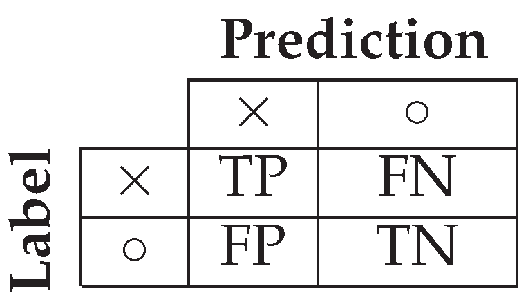
Appendix C.2. Performance Metrics
Metrics such as False Positive Rate (FPR), False Negative Rate (FNR), True Positive Rate (TPR), True Negative Rate (TNR), accuracy, precision, recall (also known as TPR), and F1-score can be derived from a confusion matrix.
- 1.
- FPR (also known as the false alarm rate (FAR)) is the proportion of normal instances incorrectly classified as anomalies. FPR =
- 2.
- FNR is the proportion of anomalies incorrectly classified as normal. FNR =
- 3.
- TNR is the proportion of normal instances correctly identified. TNR =
- 4.
- Accuracy =
- 5.
- Precision =
- 6.
- Recall (TPR or Sensitivity or Detection Rate) =
- 7.
- F1-score =
The above-defined True Positive Rate (TPR) and True Negative Rate (TNR) for anomaly detection can be adapted to evaluate Intrusion Detection Systems (IDS) as follows:
Detection rate of attack block (TPR) =
Detection rate of normal block (TNR) = ,
-
where is the number of total attack blocks, is the number of attack blocks detected by IDS, is the total number of normal blocks and is the total number of normal blocks detected by IDS [99].
- 1.
- Macro F1-score = , where N is the number of classes and is the F1-score for class i.
- 2.
- Weighted F1-score = , where N is the number of classes number of true instances in class i, n the total number of instances and is the F1-score for class i.
- 3.
- Balanced Accuracy = , which calculates the average recall for both positive and negative classes.
- 4.
- Matthews correlation coefficient (Mathews CC) = , Mathews CC is used to evaluate binary classification in imbalanced scenarios, and it ranges between -1 and +1, where +1 indicates perfect classification, 0 indicates random classification, and -1 indicates complete misclassifications.
Appendix D. Reviewed Papers Summary
60 technical papers were selected and reviewed in this survey. Table A2 and Table A3 present a summary of these works, including an overview of techniques used at each phase of the anomaly detection process.
Table A2.
Summary of Two-stage Anomaly Detection Methods. Post-detection Analysis Methods: Investigation Results (IR), Model Explanation (ME)
Table A2.
Summary of Two-stage Anomaly Detection Methods. Post-detection Analysis Methods: Investigation Results (IR), Model Explanation (ME)
| Proposed System | Data Source | Graph Used | Phase 1- Graph Pre-process, Feature Extraction and GRL | Phase 2- Anomaly Detection | Post Analysis |
|---|---|---|---|---|---|
| Xiao et al. [8] | Network | Network traffic graph | Node embedding | Classification | ✗ |
| GODIT [57] | Network | Network traffic graph | Feature extraction, Encoding | Outlier detection | ✗ |
| Munoz et al. [58] | Network | Network traffic graph | Feature extraction | Deep learning | ✗ |
| Fu et al. [55] | Network | Network traffic graph | Structural and temporal embedding | Ensemble method | ✗ |
| Gao et al. [67] | Network | Network traffic graph | Node embedding | Clustering | ✗ |
| Hu et al. [60] | Network | Network flow graph | Graph / subgraph embedding | Ensemble method | ✗ |
| Messai et al. [62] | Network | Network flow graph | Node embedding | Deep learning | ✗ |
| Friji et al. [74] | Network | Network flow graph | Data transformation, Spatial and non-spatial embeddings | Neural network | ✗ |
| DLGNN [79] | Network | Network flow graph | Structural (edge) and temporal embeding | Deep learning | ✗ |
| Anomal-E [76] | Network | Network flow graph | Edge embedding | Classification /Clustering / Outlier detection | ✗ |
| X-CBA [77] | Network | Network flow graph | Edge embedding | ML classification | ME |
| Meng et al. [51] | Network | Network logs graph | Data reduction, Feature extraction, Encoding | Outlier detection | ✗ |
| Sec2graph [19] | Network | Network logs graph | Encoding | Deep learning | ✗ |
| GenGLAD [81] | Network | Network log graph | Feature extraction, Encoding | Clustering | ✗ |
| Wrongdoing Monitor [109] | Network | Property graph | Node embedding | Classification | ✗ |
| PROVDETECTOR [7] | Host | Provenance graph | Feature extraction, Graph embedding | Clustering | ✗ |
| UNICORN [49] | Host | Provenance graph | Data transformation, Encoding | Clustering | ✗ |
| ANUBIS [46] | Host | Provenance graph | Feature extraction, Encoding | Deep learning | IR |
| PROGRAPHER [52] | Host | Provenance graph | Graph embedding | Deep learning | IR |
| EdgeTorrent [92] | Host | Provenance graph | Encoding, Node embedding | Deep learning | ✗ |
| OC-DHetGNN [103] | Host | Provenance graph | Node and graph embedding | Deep learning | ✗ |
| GCA [86] | Host | Provenance graph | Graph / subgraph embedding | Deep learning | ✗ |
| Lakha et al. [88] | Host | Provenance graph | Encoded features, Node embedding | Classification | ✗ |
| R-CAID [93] | Host | Provenance Graph | Node Embedding | Clustering | ✗ |
| Flash [89] | Host | Provenance Graph | Encoding, Node Embedding | Classification | IR |
| MAGIC [90] | Host | Provenance Graph | Node Embedding | Outlier detection | ✗ |
| Cao et al. [95] | Host | Audit data graph | Feature extraction | Classification | ✗ |
| PG-AIDS [104] | Host | Provenance Graph | Path Embedding | Deep Learning | ✗ |
| CTLMD [96] | Host | Audit data graph | Structural (node) and temporal embedding | Classification | ✗ |
| Federated GNN [98] | CAN | CAN graph | Feature generation | Autoencoder | ✗ |
| GB-IDS [106] | CAN | CAN graph | Feature generation | Graph Encoder Decoder | ✗ |
| Islam et al. [100] | CAN | CAN graph | Feature extraction | Statistical analysis | ✗ |
Table A3.
Papers Summary for End-to-end GBAD Approaches: IAR - Investigate Anomalous Results
| Proposed System | Data Source | Graph Used | End to End Anomaly Detection Approach | Post Analysis |
|---|---|---|---|---|
| TPE-NIDS [65] | Network | Network traffic graph | GNN based on edge embedding | ✗ |
| FAPDD [69] | Network | Network traffic graph | Graph kernel based | ✗ |
| Network AD [66] | Network | Network traffic graph | Graph analysis with time series analysis | ✗ |
| GTAE-IDS [70] | Network | Network traffic graph | Graph autoEncoder | ✗ |
| GRID [71] | Network | Network traffic graph | GNN with attention mechanism | ✗ |
| Villegas et al. [68] | Network | Network traffic graph | GNN | ✗ |
| AnomGraphAdv [72] | Network | Network traffic graph | Graph autoEncoder | ✗ |
| E-GraphSAGE [75] | Network | Network flow graph | GNN based on edge embedding | ✗ |
| HyperVision [73] | Network | Network flow graph | Graph clustering | ✗ |
| FeCoGraph [78] | Network | Network flow graph | GNN with contrastive learning | ✗ |
| KnowGraph [82] | Network | Network flow graph | Knowledge-enabled GNN | ✗ |
| RShield [84] | Network | Network logs graph | GNN based on node embedding | ✗ |
| Kisanga et al. [83] | Network | Network logs graph | GNN | ✗ |
| MIMC [85] | Network | Network logs graph | Graph clustering | ✗ |
| Wei et al. [12] | Network | Directed graph | GNN with structure learning | IAR |
| Attack Miner [91] | Host | Provenance graph | GNN based on attention to neighbor nodes | ✗ |
| LogTracer [87] | Host | Provenance graph | Anomaly scoring based | ✗ |
| AJSAGE [94] | Host | Provenance graph | GNN | ✗ |
| MEWRGNN [97] | Host | Audit data graph | GNN | ✗ |
| Logs2Graphs [37] | Host | Host logs graph | GNN based on nodes and edge feature learning | IAR |
| KAIROS [59] | Host | Provenance graph | GNN with a temporal model | IR |
| WSG-InV [99] | CAN | CAN graph | Subgraph analysis | ✗ |
| BERTHTLG [108] | Multi-modal | Multi-modal data graph | GNN based on anomaly scoring | ✗ |
| Li et al. [80] | Multi-modal | Network logs graph, Provenance graph | Novel attention based GNN approach | ✗ |
| MSTGAD [101] | Multi-modal | Multi-modal data graph | Graph encoder-decoder approach | ✗ |
| TraceGra [107] | Multi-modal | Multi-modal data graph | GNN with a temporal model | ✗ |
| StrGNN [63] | N/A | Dynamic graph | GNN with a temporal model | ✗ |
| TSAD [64] | N/A | Dynamic graph | Community and evolutionary based | ✗ |
| 1 |
References
- startupdaily. The DP World logistics cyber attack looks like sabotage by a ‘foreign state actor’. 2019. [Google Scholar]
- Council, A.R. DP240101547 — Griffith University. 2019. [Google Scholar]
- Zuech, R.; Khoshgoftaar, T.M.; Wald, R. Intrusion detection and big heterogeneous data: a survey. Journal of Big Data 2015, 2, 1–41. [Google Scholar] [CrossRef]
- Reports.; Data. Anomaly Detection Market. 2022.
- Azeez, N.A.; Bada, T.M.; Misra, S.; Adewumi, A.; Van der Vyver, C.; Ahuja, R. Intrusion detection and prevention systems: an updated review. Data Management, Analytics and Innovation: Proceedings of ICDMAI 2019, Volume 1 2020, pp. 685–696.
- Samrin, R.; Vasumathi, D. Review on anomaly based network intrusion detection system. In Proceedings of the 2017 international conference on electrical, electronics, communication, computer, and optimization techniques (ICEECCOT); IEEE, 2017; pp. 141–147. [Google Scholar]
- Wang, Q.; Hassan, W.U.; Li, D.; Jee, K.; Yu, X.; Zou, K.; Rhee, J.; Chen, Z.; Cheng, W.; Gunter, C.A.; et al. You Are What You Do: Hunting Stealthy Malware via Data Provenance Analysis. In Proceedings of the NDSS, 2020. [Google Scholar]
- Xiao, Q.; Liu, J.; Wang, Q.; Jiang, Z.; Wang, X.; Yao, Y. Towards network anomaly detection using graph embedding. In Proceedings of the Computational Science–ICCS 2020: 20th International Conference, Amsterdam, The Netherlands, June 3–5, 2020, Proceedings, Part IV 20; Springer, 2020; pp. 156–169. [Google Scholar]
- Garcia-Teodoro, P.; Diaz-Verdejo, J.; Maciá-Fernández, G.; Vázquez, E. Anomaly-based network intrusion detection: Techniques, systems and challenges. computers & security 2009, 28, 18–28. [Google Scholar]
- Lee, J.; Park, K. GAN-based imbalanced data intrusion detection system. Personal and Ubiquitous Computing 2021, 25, 121–128. [Google Scholar] [CrossRef]
- Zengy, J.; Wang, X.; Liu, J.; Chen, Y.; Liang, Z.; Chua, T.S.; Chua, Z.L. Shadewatcher: Recommendation-guided cyber threat analysis using system audit records. In Proceedings of the 2022 IEEE Symposium on Security and Privacy (SP); IEEE, 2022; pp. 489–506. [Google Scholar]
- Wei, C.; Xie, G.; Diao, Z. Network Flow Based IoT Anomaly Detection Using Graph Neural Network. In Proceedings of the International Conference on Knowledge Science, Engineering and Management; Springer, 2023; pp. 432–445. [Google Scholar]
- Milajerdi, S.M.; Gjomemo, R.; Eshete, B.; Sekar, R.; Venkatakrishnan, V. Holmes: real-time apt detection through correlation of suspicious information flows. In Proceedings of the 2019 IEEE Symposium on Security and Privacy (SP); IEEE, 2019; pp. 1137–1152. [Google Scholar]
- Kim, J. Studies on Inspecting Encrypted Data: Trends and Challenges. Journal of Wireless Mobile Networks, Ubiquitous Computing, and Dependable Applications (JoWUA) 2023, 189–199. [Google Scholar] [CrossRef]
- Ren, J.; Xia, F.; Lee, I.; Noori Hoshyar, A.; Aggarwal, C. Graph learning for anomaly analytics: Algorithms, applications, and challenges. ACM Transactions on Intelligent Systems and Technology 2023, 14, 1–29. [Google Scholar] [CrossRef]
- Paudel, R.; Tharp, L.; Kaiser, D.; Eberle, W.; Gannod, G. Visualization of Anomalies using Graph-Based Anomaly Detection. In Proceedings of the The International FLAIRS Conference Proceedings; 2021; Vol. 34. [Google Scholar]
- Hong, Y.; Shi, C.; Chen, J.; Wang, H.; Wang, D. Multitask Asynchronous Metalearning for Few-Shot Anomalous Node Detection in Dynamic Networks. IEEE Transactions on Computational Social Systems; 2024. [Google Scholar]
- Akoglu, L.; Tong, H.; Koutra, D. Graph-based Anomaly Detection and Description: A Survey. 2014. [Google Scholar] [CrossRef]
- Leichtnam, L.; Totel, E.; Prigent, N.; Mé, L. Sec2graph: Network attack detection based on novelty detection on graph structured data. In Proceedings of the Detection of Intrusions and Malware, and Vulnerability Assessment: 17th International Conference, DIMVA 2020, Lisbon, Portugal, June 24–26, 2020, Proceedings 17; Springer, 2020; pp. 238–258. [Google Scholar]
- Guo, D.; Liu, Z.; Li, R. RegraphGAN: A graph generative adversarial network model for dynamic network anomaly detection. Neural Networks 2023, 166, 273–285. [Google Scholar] [CrossRef] [PubMed]
- Pourhabibi, T.; Ong, K.L.; Kam, B.H.; Boo, Y.L. Fraud detection: A systematic literature review of graph-based anomaly detection approaches. Decision Support Systems 2020, 133, 113303. [Google Scholar] [CrossRef]
- Li, Z.; Chen, Q.A.; Yang, R.; Chen, Y.; Ruan, W. Threat detection and investigation with system-level provenance graphs: a survey. Computers & Security 2021, 106, 102282. [Google Scholar] [CrossRef]
- Kim, H.; Lee, B.S.; Shin, W.Y.; Lim, S. Graph anomaly detection with graph neural networks: Current status and challenges. IEEE Access 2022. [Google Scholar] [CrossRef]
- Pazho, A.D.; Noghre, G.A.; Purkayastha, A.A.; Vempati, J.; Martin, O.; Tabkhi, H. A Survey of Graph-based Deep Learning for Anomaly Detection in Distributed Systems. arXiv 2022, arXiv:2206.04149. [Google Scholar] [CrossRef]
- Lagraa, S.; Husák, M.; Seba, H.; Vuppala, S.; State, R.; Ouedraogo, M. A review on graph-based approaches for network security monitoring and botnet detection. International Journal of Information Security 2023, 1–22. [Google Scholar] [CrossRef]
- Bilot, T.; El Madhoun, N.; Al Agha, K.; Zouaoui, A. Graph Neural Networks for Intrusion Detection: A Survey. IEEE Access 2023. [Google Scholar] [CrossRef]
- Zhong, M.; Lin, M.; Zhang, C.; Xu, Z. A Survey on Graph Neural Networks for Intrusion Detection Systems: Methods, Trends and Challenges. Computers & Security 2024, 103821. [Google Scholar]
- Eltanbouly, S.; Bashendy, M.; AlNaimi, N.; Chkirbene, Z.; Erbad, A. Machine learning techniques for network anomaly detection: A survey. In Proceedings of the 2020 IEEE International Conference on Informatics, IoT, and Enabling Technologies (ICIoT); IEEE, 2020; pp. 156–162. [Google Scholar]
- Kwon, D.; Kim, H.; Kim, J.; Suh, S.C.; Kim, I.; Kim, K.J. A survey of deep learning-based network anomaly detection. Cluster Computing 2019, 22, 949–961. [Google Scholar] [CrossRef]
- Moustafa, N.; Hu, J.; Slay, J. A holistic review of network anomaly detection systems: A comprehensive survey. Journal of Network and Computer Applications 2019, 128, 33–55. [Google Scholar] [CrossRef]
- Nassif, A.B.; Talib, M.A.; Nasir, Q.; Dakalbab, F.M. Machine Learning for Anomaly Detection: A Systematic Review. 2021. [Google Scholar] [CrossRef]
- Chalapathy, R.; Chawla, S. Deep Learning for Anomaly Detection: A Survey. 2019. [Google Scholar] [CrossRef]
- Patcha, A.; Park, J.M. An overview of anomaly detection techniques: Existing solutions and latest technological trends. Computer networks 2007, 51, 3448–3470. [Google Scholar] [CrossRef]
- Genereux, S.J.; Lai, A.K.; Fowles, C.O.; Roberge, V.R.; Vigeant, G.P.; Paquet, J.R. MAIDENS: MIL-STD-1553 anomaly-based intrusion detection system using time-based histogram comparison. IEEE transactions on aerospace and electronic systems 2019, 56, 276–284. [Google Scholar] [CrossRef]
- Sensarma, D.; Sarma, S.S. A survey on different graph based anomaly detection techniques. Indian J Sci Technol 2015, 8, 1–7. [Google Scholar] [CrossRef]
- Lamichhane, P.B.; Eberle, W. Anomaly Detection in Graph Structured Data: A Survey. arXiv 2024, arXiv:2405.06172. [Google Scholar] [CrossRef]
- Li, Z.; Shi, J.; van Leeuwen, M. Graph Neural Network based Log Anomaly Detection and Explanation. arXiv 2023, arXiv:2307.00527. [Google Scholar]
- Fernandes, G.; Rodrigues, J.J.; Carvalho, L.F.; Al-Muhtadi, J.F.; Proença, M.L. A comprehensive survey on network anomaly detection. 2019. [Google Scholar] [CrossRef]
- Hajj, S.; El Sibai, R.; Bou Abdo, J.; Demerjian, J.; Makhoul, A.; Guyeux, C. Anomaly-based intrusion detection systems: The requirements, methods, measurements, and datasets. Transactions on Emerging Telecommunications Technologies 2021, 32, e4240. [Google Scholar] [CrossRef]
- Habeeb, R.A.A.; Nasaruddin, F.; Gani, A.; Hashem, I.A.T.; Ahmed, E.; Imran, M. Real-time big data processing for anomaly detection: A survey. International Journal of Information Management 2019, 45, 289–307. [Google Scholar] [CrossRef]
- Chandola, V.; Banerjee, A.; Kumar, V. Anomaly detection: A survey. ACM computing surveys (CSUR) 2009. [Google Scholar] [CrossRef]
- Ahmed, M.; Mahmood, A.N.; Hu, J. A survey of network anomaly detection techniques. Journal of Network and Computer Applications 2016, 60, 19–31. [Google Scholar] [CrossRef]
- Marnerides, A.K.; Schaeffer-Filho, A.; Mauthe, A. Traffic anomaly diagnosis in Internet backbone networks: A survey. Computer Networks 2014, 73, 224–243. [Google Scholar] [CrossRef]
- Adhikari, D.; Jiang, W.; Zhan, J.; Rawat, D.B.; Bhattarai, A. Recent advances in anomaly detection in Internet of Things: Status, challenges, and perspectives. Computer Science Review 2024, 54, 100665. [Google Scholar] [CrossRef]
- Anagnostopoulos, C. Weakly supervised learning: how to engineer labels for machine learning in cyber-security. In Data Science for Cyber-Security; World Scientific, 2019; pp. 195–226. [Google Scholar]
- Anjum, M.M.; Iqbal, S.; Hamelin, B. ANUBIS: a provenance graph-based framework for advanced persistent threat detection. In Proceedings of the Proceedings of the 37th ACM/SIGAPP Symposium on Applied Computing; 2022; pp. 1684–1693. [Google Scholar]
- Pang, G.; Shen, C.; Cao, L.; Hengel, A.V.D. Deep learning for anomaly detection: A review. ACM computing surveys (CSUR) 2021, 54, 1–38. [Google Scholar] [CrossRef]
- Khraisat, A.; Gondal, I.; Vamplew, P.; Kamruzzaman, J. Survey of intrusion detection systems: techniques, datasets and challenges. Cybersecurity 2019, 2, 1–22. [Google Scholar] [CrossRef]
- Han, X.; Pasquier, T.; Bates, A.; Mickens, J.; Seltzer, M. Unicorn: Runtime provenance-based detector for advanced persistent threats. arXiv 2020, arXiv:2001.01525. [Google Scholar] [CrossRef]
- Lanvin, M.; Gimenez, P.F.; Han, Y.; Majorczyk, F.; Mé, L.; Totel, É. Detecting APT through graph anomaly detection. In Proceedings of the RESSI 2022-Rendez-Vous de la Recherche et de l’Enseignement de la Sécurité des Systèmes d’Information; 2022; pp. 1–3. [Google Scholar]
- Meng, Q.; Wang, H.; Oo, N.; Lim, H.W.; Schätz, B.J.; Sikdar, B. Graph-Based Attack Path Discovery for Network Security. [CrossRef]
- Yang, F.; Xu, J.; Xiong, C.; Li, Z.; Zhang, K. {PROGRAPHER}: An Anomaly Detection System based on Provenance Graph Embedding. In Proceedings of the 32nd USENIX Security Symposium (USENIX Security 23); 2023; pp. 4355–4372. [Google Scholar]
- Jain, P.; Jain, S.; Zaïane, O.R.; Srivastava, A. Anomaly detection in resource constrained environments with streaming data. IEEE Transactions on Emerging Topics in Computational Intelligence 2021, 6, 649–659. [Google Scholar] [CrossRef]
- Ouarbya, L.; Rahul, M. Interpretable Anomaly Detection: A Hybrid Approach Using Rule-Based and Machine Learning Techniques. 2023. [Google Scholar] [CrossRef]
- Fu, Z.; Liu, M.; Qin, Y.; Zhang, J.; Zou, Y.; Yin, Q.; Li, Q.; Duan, H. Encrypted malware traffic detection via graph-based network analysis. In Proceedings of the Proceedings of the 25th International Symposium on Research in Attacks, Intrusions and Defenses; 2022; pp. 495–509. [Google Scholar]
- Xing, J.; Wu, C. Detecting anomalies in encrypted traffic via deep dictionary learning. In Proceedings of the IEEE INFOCOM 2020-IEEE Conference on Computer Communications Workshops (INFOCOM WKSHPS); IEEE, 2020; pp. 734–739. [Google Scholar]
- Paudel, R.; Muncy, T.; Eberle, W. Detecting dos attack in smart home iot devices using a graph-based approach. In Proceedings of the 2019 IEEE international conference on big data (big data); IEEE, 2019; pp. 5249–5258. [Google Scholar]
- Muñoz, D.C.; Valiente, A.d.C. A novel botnet attack detection for IoT networks based on communication graphs. Cybersecurity 2023, 6, 33. [Google Scholar] [CrossRef]
- Cheng, Z.; Lv, Q.; Liang, J.; Wang, Y.; Sun, D.; Pasquier, T.; Han, X. KAIROS: practical intrusion detection and investigation using whole-system provenance. In Proceedings of the 2024 IEEE Symposium on Security and Privacy (SP); IEEE, 2024; pp. 3533–3551. [Google Scholar]
- Hu, X.; Gao, W.; Cheng, G.; Li, R.; Zhou, Y.; Wu, H. Towards Early and Accurate Network Intrusion Detection Using Graph Embedding. IEEE Transactions on Information Forensics and Security 2023. [Google Scholar] [CrossRef]
- Yu, L.; Tao, J.; Xu, Y.; Sun, W.; Wang, Z. TLS fingerprint for encrypted malicious traffic detection with attributed graph kernel. Computer Networks 2024, 247, 110475. [Google Scholar] [CrossRef]
- Messai, M.L.; Seba, H. IoT Network Attack Detection: Leveraging Graph Learning for Enhanced Security. In Proceedings of the Proceedings of the 18th International Conference on Availability, Reliability and Security; 2023; pp. 1–7. [Google Scholar]
- Cai, L.; Chen, Z.; Luo, C.; Gui, J.; Ni, J.; Li, D.; Chen, H. Structural temporal graph neural networks for anomaly detection in dynamic graphs. In Proceedings of the Proceedings of the 30th ACM international conference on Information & Knowledge Management; 2021; pp. 3747–3756. [Google Scholar]
- Jiang, Y.; Liu, G. Two-stage anomaly detection algorithm via dynamic community evolution in temporal graph. Applied Intelligence 2022, 52, 12222–12240. [Google Scholar] [CrossRef]
- Zhang, Y.; Zhang, Y.; Wu, Y.; Li, C. TPE-NIDS: uses graph neural networks to detect malicious traffic. In Proceedings of the 2022 4th International Conference on Frontiers Technology of Information and Computer (ICFTIC); IEEE, 2022; pp. 949–958. [Google Scholar]
- Tsikerdekis, M.; Waldron, S.; Emanuelson, A. Network anomaly detection using exponential random graph models and autoregressive moving average. IEEE Access 2021, 9, 134530–134542. [Google Scholar] [CrossRef]
- Gao, M.; Wu, L.; Li, Q.; Chen, W. Anomaly traffic detection in IoT security using graph neural networks. Journal of Information Security and Applications 2023, 76, 103532. [Google Scholar] [CrossRef]
- Villegas-Ch, W.; Govea, J.; Navarro, A.M.; Játiva, P.P. Intrusion Detection in IoT Networks Using Dynamic Graph Modeling and Graph-Based Neural Networks. IEEE Access 2025. [Google Scholar] [CrossRef]
- Liu, X.; Ren, J.; He, H.; Zhang, B.; Song, C.; Wang, Y. A fast all-packets-based DDoS attack detection approach based on network graph and graph kernel. Journal of Network and Computer Applications 2021, 185, 103079. [Google Scholar] [CrossRef]
- Ghadermazi, J.; Hore, S.; Shah, A.; Bastian, N.D. GTAE-IDS: Graph Transformer-based Autoencoder Framework for Real-time Network Intrusion Detection. IEEE Transactions on Information Forensics and Security 2025. [Google Scholar] [CrossRef]
- Kong, X.; Song, Z.; Ye, X.; Jiao, J.; Qi, H.; Liu, X. GRID: Graph-Based Robust Intrusion Detection Solution for Industrial IoT Networks. IEEE Internet of Things Journal 2025. [Google Scholar] [CrossRef]
- Bajpai, S.; Krishna Murthy, P.; Kumar, N. AnomGraphAdv: Enhancing Anomaly and Network Intrusion Detection in Wireless Networks Using Adversarial Training and Temporal Graph Networks. In Proceedings of the Proceedings of the 17th ACM Conference on Security and Privacy in Wireless and Mobile Networks; 2024; pp. 113–122. [Google Scholar]
- Fu, C.; Li, Q.; Xu, K. Detecting unknown encrypted malicious traffic in real time via flow interaction graph analysis. arXiv 2023, arXiv:2301.13686. [Google Scholar] [CrossRef]
- Friji, H.; Olivereau, A.; Sarkiss, M. Efficient Network Representation for GNN-Based Intrusion Detection. In Proceedings of the International Conference on Applied Cryptography and Network Security; Springer, 2023; pp. 532–554. [Google Scholar]
- Lo, W.W.; Layeghy, S.; Sarhan, M.; Gallagher, M.; Portmann, M. E-graphsage: A graph neural network based intrusion detection system for iot. In Proceedings of the NOMS 2022-2022 IEEE/IFIP Network Operations and Management Symposium; IEEE, 2022; pp. 1–9. [Google Scholar]
- Caville, E.; Lo, W.W.; Layeghy, S.; Portmann, M. Anomal-E: A self-supervised network intrusion detection system based on graph neural networks. Knowledge-based systems 2022, 258, 110030. [Google Scholar] [CrossRef]
- Kaya, K.; Ak, E.; Bas, S.; Canberk, B.; Oguducu, S.G. X-CBA: Explainability Aided CatBoosted Anomal-E for Intrusion Detection System. arXiv 2024, arXiv:2402.00839. [Google Scholar]
- Mao, Q.; Lin, X.; Xu, W.; Qi, Y.; Su, X.; Li, G.; Li, J. FeCoGraph: Label-aware Federated Graph Contrastive Learning for Few-shot Network Intrusion Detection. IEEE Transactions on Information Forensics and Security 2025. [Google Scholar] [CrossRef]
- Duan, G.; Lv, H.; Wang, H.; Feng, G. Application of a dynamic line graph neural network for intrusion detection with semisupervised learning. IEEE Transactions on Information Forensics and Security 2022, 18, 699–714. [Google Scholar] [CrossRef]
- Li, Z.; Cheng, X.; Sun, L.; Zhang, J.; Chen, B. A hierarchical approach for advanced persistent threat detection with attention-based graph neural networks. Security and Communication Networks 2021, 2021, 1–14. [Google Scholar] [CrossRef]
- Wang, H.; Chen, Y.; Zhang, C.; Li, J.; Gan, C.; Zhang, Y.; Chen, X. GenGLAD: A Generated Graph Based Log Anomaly Detection Framework. In Proceedings of the International Conference on Smart Computing and Communication; Springer, 2022; pp. 11–22. [Google Scholar]
- Zhou, A.; Xu, X.; Raghunathan, R.; Lal, A.; Guan, X.; Yu, B.; Li, B. KnowGraph: Knowledge-Enabled Anomaly Detection via Logical Reasoning on Graph Data. In Proceedings of the Proceedings of the 2024 on ACM SIGSAC Conference on Computer and Communications Security; 2024; pp. 168–182. [Google Scholar]
- Kisanga, P.; Woungang, I.; Traore, I.; Carvalho, G.H. Network Anomaly Detection Using a Graph Neural Network. In Proceedings of the 2023 International Conference on Computing, Networking and Communications (ICNC); IEEE, 2023; pp. 61–65. [Google Scholar]
- Yang, W.; Gao, P.; Huang, H.; Wei, X.; Liu, W.; Zhu, S.; Luo, W. RShield: A refined shield for complex multi-step attack detection based on temporal graph network. In Proceedings of the International Conference on Database Systems for Advanced Applications; Springer, 2022; pp. 468–480. [Google Scholar]
- Copstein, R.; Niblett, B.; Johnston, A.; Schwartzentruber, J.; Heywood, M.; Zincir-Heywood, N. Towards Anomaly Detection using Multiple Instances of Micro-Cluster Detection. In Proceedings of the 2023 7th Cyber Security in Networking Conference (CSNet); IEEE, 2023; pp. 185–191. [Google Scholar]
- Ye, M.; Men, S.; Xie, L.; Chen, B. Detect Advanced Persistent Threat In Graph-Level Using Competitive AutoEncoder. In Proceedings of the Proceedings of the 2023 2nd International Conference on Networks, Communications and Information Technology; 2023; pp. 28–34. [Google Scholar]
- Niu, W.; Yu, Z.; Li, Z.; Li, B.; Zhang, R.; Zhang, X. LogTracer: Efficient Anomaly Tracing Combining System Log Detection and Provenance Graph. In Proceedings of the GLOBECOM 2022-2022 IEEE Global Communications Conference; IEEE, 2022; pp. 3356–3361. [Google Scholar]
- Lakha, B.; Mount, S.L.; Serra, E.; Cuzzocrea, A. Anomaly Detection in Cybersecurity Events Through Graph Neural Network and Transformer Based Model: A Case Study with BETH Dataset. In Proceedings of the 2022 IEEE International Conference on Big Data (Big Data); IEEE, 2022; pp. 5756–5764. [Google Scholar]
- Rehman, M.U.; Ahmadi, H.; Hassan, W.U. Flash: A comprehensive approach to intrusion detection via provenance graph representation learning. In Proceedings of the 2024 IEEE Symposium on Security and Privacy (SP); IEEE, 2024; pp. 3552–3570. [Google Scholar]
- Jia, Z.; Xiong, Y.; Nan, Y.; Zhang, Y.; Zhao, J.; Wen, M. {MAGIC}: Detecting advanced persistent threats via masked graph representation learning. In Proceedings of the 33rd USENIX Security Symposium (USENIX Security 24); 2024; pp. 5197–5214. [Google Scholar]
- Pan, Y.; Cai, L.; Leng, T.; Zhao, L.; Ma, J.; Yu, A.; Meng, D. AttackMiner: A Graph Neural Network Based Approach for Attack Detection from Audit Logs. In Proceedings of the International Conference on Security and Privacy in Communication Systems; Springer, 2022; pp. 510–528. [Google Scholar]
- King, I.J.; Shu, X.; Jang, J.; Eykholt, K.; Lee, T.; Huang, H.H. EdgeTorrent: Real-time Temporal Graph Representations for Intrusion Detection. In Proceedings of the Proceedings of the 26th International Symposium on Research in Attacks, Intrusions and Defenses; 2023; pp. 77–91. [Google Scholar]
- Goyal, A.; Wang, G.; Bates, A. R-caid: Embedding root cause analysis within provenance-based intrusion detection. In Proceedings of the 2024 IEEE Symposium on Security and Privacy (SP); IEEE, 2024; pp. 3515–3532. [Google Scholar]
- Xu, L.; Zhao, Z.; Zhao, D.; Li, X.; Lu, X.; Yan, D. AJSAGE: A intrusion detection scheme based on Jump-Knowledge Connection To GraphSAGE. Computers & Security 2025, 150, 104263. [Google Scholar]
- Cao, Z.; Stephen Huang, S.H. Host-Based Intrusion Detection: A Behavioral Approach Using Graph Model. In Proceedings of the International Conference on Hybrid Intelligent Systems; Springer, 2022; pp. 1337–1346. [Google Scholar]
- Zhao, S.; Wei, R.; Cai, L.; Yu, A.; Meng, D. Ctlmd: Continuous-temporal lateral movement detection using graph embedding. In Proceedings of the Information and Communications Security: 21st International Conference, ICICS 2019, Beijing, China, December 15–17, 2019, Revised Selected Papers 21. Springer, 2020; pp. 181–196. [Google Scholar]
- Xiao, J.; Yang, L.; Zhong, F.; Wang, X.; Chen, H.; Li, D. Robust Anomaly-based Insider Threat Detection using Graph Neural Network. IEEE Transactions on Network and Service Management 2022. [Google Scholar] [CrossRef]
- Zhang, H.; Zeng, K.; Lin, S. Federated graph neural network for fast anomaly detection in controller area networks. IEEE Transactions on Information Forensics and Security 2023, 18, 1566–1579. [Google Scholar] [CrossRef]
- Linghu, Y.; Li, X. Wsg-inv: Weighted state graph model for intrusion detection on in-vehicle network. In Proceedings of the 2021 IEEE Wireless Communications and Networking Conference (WCNC); IEEE, 2021; pp. 1–7. [Google Scholar]
- Islam, R.; Refat, R.U.D.; Yerram, S.M.; Malik, H. Graph-based intrusion detection system for controller area networks. IEEE Transactions on Intelligent Transportation Systems 2020, 23, 1727–1736. [Google Scholar] [CrossRef]
- Huang, J.; Yang, Y.; Yu, H.; Li, J.; Zheng, X. Twin Graph-Based Anomaly Detection via Attentive Multi-Modal Learning for Microservice System. In Proceedings of the 2023 38th IEEE/ACM International Conference on Automated Software Engineering (ASE); IEEE, 2023; pp. 66–78. [Google Scholar]
- Liu, T.; Li, Z.; Long, H.; Bilal, A. Nt-gnn: Network traffic graph for 5g mobile iot android malware detection. Electronics 2023, 12, 789. [Google Scholar] [CrossRef]
- Huang, Z.; Gu, Y.; Zhao, Q. One-Class Directed Heterogeneous Graph Neural Network for Intrusion Detection. In Proceedings of the 2022 the 6th International Conference on Innovation in Artificial Intelligence (ICIAI); 2022; pp. 178–184. [Google Scholar]
- Meng, L.; Xi, R.; Li, Z.; Zhu, H. PG-AID: An Anomaly-based Intrusion Detection Method Using Provenance Graph. In Proceedings of the 2024 27th International Conference on Computer Supported Cooperative Work in Design (CSCWD); IEEE, 2024; pp. 2522–2527. [Google Scholar]
- Pennington, J.; Socher, R.; Manning, C.D. Glove: Global vectors for word representation. In Proceedings of the Proceedings of the 2014 conference on empirical methods in natural language processing (EMNLP); 2014; pp. 1532–1543. [Google Scholar]
- Meng, Y.; Li, J.; Liu, F.; Li, S.; Hu, H.; Zhu, H. GB-IDS: An Intrusion Detection System for CAN Bus Based on Graph Analysis. In Proceedings of the 2023 IEEE/CIC International Conference on Communications in China (ICCC); IEEE, 2023; pp. 1–6. [Google Scholar]
- Chen, J.; Liu, F.; Jiang, J.; Zhong, G.; Xu, D.; Tan, Z.; Shi, S. TraceGra: A trace-based anomaly detection for microservice using graph deep learning. Computer Communications 2023, 204, 109–117. [Google Scholar] [CrossRef]
- Chen, L.; Dang, Q.; Chen, M.; Sun, B.; Du, C.; Lu, Z. BertHTLG: Graph-Based Microservice Anomaly Detection Through Sentence-Bert Enhancement. In Proceedings of the International Conference on Web Information Systems and Applications; Springer, 2023; pp. 427–439. [Google Scholar]
- Wang, C.; Zhu, H. Wrongdoing monitor: a graph-based behavioral anomaly detection in cyber Security. IEEE Transactions on Information Forensics and Security 2022, 17, 2703–2718. [Google Scholar] [CrossRef]
- Deng, D. DBSCAN clustering algorithm based on density. In Proceedings of the 2020 7th international forum on electrical engineering and automation (IFEEA); IEEE, 2020; pp. 949–953. [Google Scholar]
- Paudel, R.; Eberle, W. Snapsketch: Graph representation approach for intrusion detection in a streaming graph. In Proceedings of the Proceedings of the 16th International Workshop on Mining and Learning with Graphs (MLG); 2020. [Google Scholar]
- Shi, H.; Li, H.; Zhang, D.; Cheng, C.; Cao, X. An efficient feature generation approach based on deep learning and feature selection techniques for traffic classification. Computer Networks 2018, 132, 81–98. [Google Scholar] [CrossRef]
- Eswaran, D.; Faloutsos, C.; Guha, S.; Mishra, N. Spotlight: Detecting anomalies in streaming graphs. In Proceedings of the Proceedings of the 24th ACM SIGKDD international conference on knowledge discovery & data mining; 2018; pp. 1378–1386. [Google Scholar]
- Lamichhane, P.B.; Eberle, W. Anomaly detection in edge streams using term frequency-inverse graph frequency (tf-igf) concept. In Proceedings of the 2021 IEEE international conference on big data (Big Data); IEEE, 2021; pp. 661–667. [Google Scholar]
- Cai, H.; Zheng, V.W.; Chang, K.C.C. A comprehensive survey of graph embedding: Problems, techniques, and applications. IEEE transactions on knowledge and data engineering 2018, 30, 1616–1637. [Google Scholar] [CrossRef]
- Zhou, J.; Cui, G.; Hu, S.; Zhang, Z.; Yang, C.; Liu, Z.; Wang, L.; Li, C.; Sun, M. Graph neural networks: A review of methods and applications. AI open 2020, 1, 57–81. [Google Scholar] [CrossRef]
- Zaccagnino, R.; Cirillo, A.; Guarino, A.; Lettieri, N.; Malandrino, D.; Zaccagnino, G. Towards a Geometric Deep Learning-Based Cyber Security: Network System Intrusion Detection Using Graph Neural Networks. In Proceedings of the SECRYPT; 2023; pp. 394–401. [Google Scholar]
- Gao, M.; Chen, L.; He, X.; Zhou, A. Bine: Bipartite network embedding. In Proceedings of the The 41st international ACM SIGIR conference on research & development in information retrieval; 2018; pp. 715–724. [Google Scholar]
- Khemani, B.; Patil, S.; Kotecha, K.; Tanwar, S. A review of graph neural networks: concepts, architectures, techniques, challenges, datasets, applications, and future directions. Journal of Big Data 2024, 11, 18. [Google Scholar] [CrossRef]
- Gilmer, J.; Schoenholz, S.S.; Riley, P.F.; Vinyals, O.; Dahl, G.E. Neural message passing for quantum chemistry. In Proceedings of the International conference on machine learning; PMLR, 2017; pp. 1263–1272. [Google Scholar]
- Mohan, A.; Pramod, K. Temporal network embedding using graph attention network. Complex & Intelligent Systems 2022, 8, 13–27. [Google Scholar]
- Hamilton, W.; Ying, Z.; Leskovec, J. Inductive representation learning on large graphs. Advances in neural information processing systems 2017, 30. [Google Scholar]
- Feng, M.H.; Hsu, C.C.; Li, C.T.; Yeh, M.Y.; Lin, S.D. Marine: Multi-relational network embeddings with relational proximity and node attributes. In Proceedings of the The World Wide Web Conference; 2019; pp. 470–479. [Google Scholar]
- Deng, A.; Hooi, B. Graph neural network-based anomaly detection in multivariate time series. Proceedings of the Proceedings of the AAAI conference on artificial intelligence 2021, 35, 4027–4035. [Google Scholar] [CrossRef]
- Purnama, S.R.; Istiyanto, J.E.; Amrizal, M.A.; Handika, V.; Rochman, S.; Dharmawan, A. Inductive Graph Neural Network with Causal Sampling for IoT Network Intrusion Detection System. In Proceedings of the 2022 International Conference on Computer Engineering, Network, and Intelligent Multimedia (CENIM); IEEE, 2022; pp. 241–246. [Google Scholar]
- Narayanan, A.; Chandramohan, M.; Venkatesan, R.; Chen, L.; Liu, Y.; Jaiswal, S. graph2vec: Learning distributed representations of graphs. arXiv 2017, arXiv:1707.05005. [Google Scholar] [CrossRef]
- Sun, F.Y.; Hoffmann, J.; Verma, V.; Tang, J. Infograph: Unsupervised and semi-supervised graph-level representation learning via mutual information maximization. arXiv 2019, arXiv:1908.01000. [Google Scholar]
- Zohrevand, Z.; Glässer, U. Should i raise the red flag? A comprehensive survey of anomaly scoring methods toward mitigating false alarms. arXiv 2019, arXiv:1904.06646. [Google Scholar]
- Eswaran, D.; Faloutsos, C. Sedanspot: Detecting anomalies in edge streams. In Proceedings of the 2018 IEEE International conference on data mining (ICDM); IEEE, 2018; pp. 953–958. [Google Scholar]
- Bu, Z.; Ye, S. Comparison of Different Partition Clustering Algorithms under the Network Flow Detection Scenario. In Proceedings of the 2024 8th International Conference on Communication and Information Systems (ICCIS); IEEE, 2024; pp. 140–144. [Google Scholar]
- Bhattarai, B.; Huang, H.H. Prov2vec: Learning provenance graph representation for anomaly detection in computer systems. In Proceedings of the Proceedings of the 19th International Conference on Availability, Reliability and Security; 2024; pp. 1–14. [Google Scholar]
- Ersoy, P. Evolution of Outlier Algorithms for Anomaly Detection. Manchester Journal of Artificial Intelligence and Applied Sciences 2021, 2. [Google Scholar]
- Gogoi, P.; Bhattacharyya, D.K.; Borah, B.; Kalita, J.K. A survey of outlier detection methods in network anomaly identification. The Computer Journal 2011, 54, 570–588. [Google Scholar] [CrossRef]
- Ma, X.; Wu, J.; Xue, S.; Yang, J.; Zhou, C.; Sheng, Q.Z.; Xiong, H.; Akoglu, L. A comprehensive survey on graph anomaly detection with deep learning. IEEE Transactions on Knowledge and Data Engineering 2021. [Google Scholar] [CrossRef]
- Chen, Z.; Yeo, C.K.; Lee, B.S.; Lau, C.T. Autoencoder-based network anomaly detection. In Proceedings of the 2018 Wireless telecommunications symposium (WTS); IEEE, 2018; pp. 1–5. [Google Scholar]
- Samariya, D.; Thakkar, A. A comprehensive survey of anomaly detection algorithms. Annals of Data Science 2023, 10, 829–850. [Google Scholar] [CrossRef]
- Thomas, J.M.; Moallemy-Oureh, A.; Beddar-Wiesing, S.; Holzhüter, C. Graph neural networks designed for different graph types: A survey. arXiv 2022, arXiv:2204.03080. [Google Scholar]
- Ruff, L.; Vandermeulen, R.; Goernitz, N.; Deecke, L.; Siddiqui, S.A.; Binder, A.; Müller, E.; Kloft, M. Deep one-class classification. In Proceedings of the International conference on machine learning; PMLR, 2018; pp. 4393–4402. [Google Scholar]
- Xu, K.; Li, C.; Tian, Y.; Sonobe, T.; Kawarabayashi, K.i.; Jegelka, S. Representation learning on graphs with jumping knowledge networks. In Proceedings of the International conference on machine learning; PMLR, 2018; pp. 5453–5462. [Google Scholar]
- Bui, K.H.N.; Cho, J.; Yi, H. Spatial-temporal graph neural network for traffic forecasting: An overview and open research issues. Applied Intelligence 2022, 52, 2763–2774. [Google Scholar] [CrossRef]
- Rossi, E.; Chamberlain, B.; Frasca, F.; Eynard, D.; Monti, F.; Bronstein, M. Temporal graph networks for deep learning on dynamic graphs. arXiv 2020, arXiv:2006.10637. [Google Scholar] [CrossRef]
- Bhatia, S.; Liu, R.; Hooi, B.; Yoon, M.; Shin, K.; Faloutsos, C. Real-time anomaly detection in edge streams. ACM Transactions on Knowledge Discovery from Data (TKDD) 2022, 16, 1–22. [Google Scholar] [CrossRef]
- Sharafaldin, I.; Lashkari, A.H.; Ghorbani, A.A.; et al. Toward generating a new intrusion detection dataset and intrusion traffic characterization. ICISSp 2018, 1, 108–116. [Google Scholar]
- Moustafa, N.; Slay, J. UNSW-NB15: a comprehensive data set for network intrusion detection systems (UNSW-NB15 network data set). In Proceedings of the 2015 military communications and information systems conference (MilCIS); IEEE, 2015; pp. 1–6. [Google Scholar]
- Sahoo, K.S.; Puthal, D.; Tiwary, M.; Rodrigues, J.J.; Sahoo, B.; Dash, R. An early detection of low rate DDoS attack to SDN based data center networks using information distance metrics. Future Generation Computer Systems 2018, 89, 685–697. [Google Scholar] [CrossRef]
- Garcia, S.; Grill, M.; Stiborek, J.; Zunino, A. An empirical comparison of botnet detection methods. computers & security 2014, 45, 100–123. [Google Scholar]
- Song, J.; Takakura, H.; Okabe, Y.; Eto, M.; Inoue, D.; Nakao, K. Statistical analysis of honeypot data and building of Kyoto 2006+ dataset for NIDS evaluation. In Proceedings of the Proceedings of the first workshop on building analysis datasets and gathering experience returns for security; 2011; pp. 29–36. [Google Scholar]
- Lashkari, A.H.; Gil, G.D.; Mamun, M.S.I.; Ghorbani, A.A. Characterization of tor traffic using time based features. In Proceedings of the International Conference on Information Systems Security and Privacy; SciTePress, 2017; Vol. 2, pp. 253–262. [Google Scholar]
- Lukaseder, T. 2017-SUEE-data-set, 2017.
- Taheri, L.; Kadir, A.F.A.; Lashkari, A.H. Extensible android malware detection and family classification using network-flows and API-calls. In Proceedings of the 2019 international Carnahan conference on security technology (ICCST); IEEE, 2019; pp. 1–8. [Google Scholar]
- Kolias, C.; Kambourakis, G.; Stavrou, A.; Gritzalis, S. Intrusion detection in 802.11 networks: Empirical evaluation of threats and a public dataset. IEEE Communications Surveys & Tutorials 2015, 18, 184–208. [Google Scholar] [CrossRef]
- Glasser, J.; Lindauer, B. Bridging the gap: A pragmatic approach to generating insider threat data. In Proceedings of the 2013 IEEE Security and Privacy Workshops. IEEE; 2013; pp. 98–104. [Google Scholar]
- Koroniotis, N.; Moustafa, N.; Sitnikova, E.; Turnbull, B. Towards the development of realistic botnet dataset in the internet of things for network forensic analytics: Bot-iot dataset. Future Generation Computer Systems 2019, 100, 779–796. [Google Scholar] [CrossRef]
- Sarhan, M.; Layeghy, S.; Moustafa, N.; Portmann, M. Netflow datasets for machine learning-based network intrusion detection systems. In Proceedings of the Big Data Technologies and Applications: 10th EAI International Conference, BDTA 2020, and 13th EAI International Conference on Wireless Internet, WiCON 2020, Virtual Event, December 11, 2020, Proceedings 10; Springer, 2021; pp. 117–135. [Google Scholar]
- Saad, S.; Traore, I.; Ghorbani, A.; Sayed, B.; Zhao, D.; Lu, W.; Felix, J.; Hakimian, P. Detecting P2P botnets through network behavior analysis and machine learning. In Proceedings of the 2011 Ninth annual international conference on privacy, security and trust; IEEE, 2011; pp. 174–180. [Google Scholar]
- Nack, E.A.; McKenzie, M.C.; Bastian, N.D. ACI-IoT-2023: A Robust Dataset for Internet of Things Network Security Analysis. In Proceedings of the MILCOM 2024-2024 IEEE Military Communications Conference (MILCOM); IEEE, 2024; pp. 1–6. [Google Scholar]
- Neto, E.C.P.; Dadkhah, S.; Ferreira, R.; Zohourian, A.; Lu, R.; Ghorbani, A.A. CICIoT2023: A real-time dataset and benchmark for large-scale attacks in IoT environment. Sensors 2023, 23, 5941. [Google Scholar] [CrossRef]
- Song, H.M.; Kim, H.K. Discovering can specification using on-board diagnostics. IEEE Design & Test 2020, 38, 93–103. [Google Scholar] [CrossRef]
- Lee, H.; Jeong, S.H.; Kim, H.K. OTIDS: A novel intrusion detection system for in-vehicle network by using remote frame. In Proceedings of the 2017 15th Annual Conference on Privacy, Security and Trust (PST); IEEE, 2017; pp. 57–5709. [Google Scholar]
- Camina, J.B.; Hernández-Gracidas, C.; Monroy, R.; Trejo, L. The Windows-Users and-Intruder simulations Logs dataset (WUIL): An experimental framework for masquerade detection mechanisms. Expert Systems with Applications 2014, 41, 919–930. [Google Scholar] [CrossRef]
- Alsaheel, A.; Nan, Y.; Ma, S.; Yu, L.; Walkup, G.; Celik, Z.B.; Zhang, X.; Xu, D. {ATLAS}: A sequence-based learning approach for attack investigation. In Proceedings of the 30th USENIX Security Symposium (USENIX Security 21); 2021; pp. 3005–3022. [Google Scholar]
- Manzoor, E.; Milajerdi, S.M.; Akoglu, L. Fast memory-efficient anomaly detection in streaming heterogeneous graphs. In Proceedings of the Proceedings of the 22nd ACM SIGKDD international conference on knowledge discovery and data mining; 2016; pp. 1035–1044. [Google Scholar]
- Turcotte, M.J.; Kent, A.D.; Hash, C. Unified host and network data set. In Data science for cyber-security; World Scientific, 2019; pp. 1–22. [Google Scholar]
- Zhang, C.; Peng, X.; Sha, C.; Zhang, K.; Fu, Z.; Wu, X.; Lin, Q.; Zhang, D. Deeptralog: Trace-log combined microservice anomaly detection through graph-based deep learning. In Proceedings of the Proceedings of the 44th International Conference on Software Engineering; 2022; pp. 623–634. [Google Scholar]
- Highnam, K.; Arulkumaran, K.; Hanif, Z.; Jennings, N.R. Beth dataset: Real cybersecurity data for unsupervised anomaly detection research. In Proceedings of the CEUR Workshop Proc; 2021; Vol. 3095, pp. 1–12. [Google Scholar]
- Nedelkoski, S.; Bogatinovski, J.; Mandapati, A.K.; Becker, S.; Cardoso, J.; Kao, O. Multi-source distributed system data for ai-powered analytics. In Proceedings of the Service-Oriented and Cloud Computing: 8th IFIP WG 2.14 European Conference, ESOCC 2020, Heraklion, Crete, Greece, September 28–30, 2020, Proceedings 8; Springer, 2020; pp. 161–176. [Google Scholar]
- Li, Z.; Chen, J.; Jiao, R.; Zhao, N.; Wang, Z.; Zhang, S.; Wu, Y.; Jiang, L.; Yan, L.; Wang, Z.; et al. Practical root cause localization for microservice systems via trace analysis. In Proceedings of the 2021 IEEE/ACM 29th International Symposium on Quality of Service (IWQOS); IEEE, 2021; pp. 1–10. [Google Scholar]
- Kovács, G.; Sebestyen, G.; Hangan, A. Evaluation metrics for anomaly detection algorithms in time-series. Acta Universitatis Sapientiae, Informatica 2019, 11, 113–130. [Google Scholar] [CrossRef]
- Sørbø, S.; Ruocco, M. Navigating the metric maze: a taxonomy of evaluation metrics for anomaly detection in time series. Data Mining and Knowledge Discovery 2024, 38, 1027–1068. [Google Scholar] [CrossRef]
- Sauka, K.; Shin, G.Y.; Kim, D.W.; Han, M.M. Adversarial robust and explainable network intrusion detection systems based on deep learning. Applied Sciences 2022, 12, 6451. [Google Scholar] [CrossRef]
- Liu, Y.; Ding, K.; Lu, Q.; Li, F.; Zhang, L.Y.; Pan, S. Towards Self-Interpretable Graph-Level Anomaly Detection. arXiv 2023, arXiv:2310.16520. [Google Scholar]
- Neupane, S.; Ables, J.; Anderson, W.; Mittal, S.; Rahimi, S.; Banicescu, I.; Seale, M. Explainable intrusion detection systems (x-ids): A survey of current methods, challenges, and opportunities. IEEE Access 2022, 10, 112392–112415. [Google Scholar] [CrossRef]
- Ying, Z.; Bourgeois, D.; You, J.; Zitnik, M.; Leskovec, J. Gnnexplainer: Generating explanations for graph neural networks. Advances in neural information processing systems 2019, 32. [Google Scholar]
- Holdijk, L.; Boon, M.; Henckens, S.; de Jong, L. [Re] parameterized explainer for graph neural network. In Proceedings of the ML Reproducibility Challenge 2020; 2021. [Google Scholar]
- Wang, H.; Liu, T.; Sheng, Z.; Li, H. Explanatory subgraph attacks against Graph Neural Networks. Neural Networks 2024, 172, 106097. [Google Scholar] [CrossRef] [PubMed]
- Herath, J.D.; Wakodikar, P.P.; Yang, P.; Yan, G. Cfgexplainer: Explaining graph neural network-based malware classification from control flow graphs. In Proceedings of the 2022 52nd Annual IEEE/IFIP International Conference on Dependable Systems and Networks (DSN); IEEE, 2022; pp. 172–184. [Google Scholar]
- Mukherjee, K.; Wiedemeier, J.; Wang, T.; Kim, M.; Chen, F.; Kantarcioglu, M.; Jee, K. Interpreting gnn-based ids detections using provenance graph structural features. arXiv 2023, arXiv:2306.00934. [Google Scholar] [CrossRef]
- Baahmed, A.R.E.M.; Andresini, G.; Robardet, C.; Appice, A. Using graph neural networks for the detection and explanation of network intrusions. In Proceedings of the International Workshop on eXplainable Knowledge Discovery in Data Mining; 2023. [Google Scholar]
- Sharma, J.; Giri, C.; Granmo, O.C.; Goodwin, M. Multi-layer intrusion detection system with ExtraTrees feature selection, extreme learning machine ensemble, and softmax aggregation. EURASIP Journal on Information Security 2019, 2019, 1–16. [Google Scholar] [CrossRef]
- Wang, Y.; Liu, Z.; Zheng, W.; Wang, J.; Shi, H.; Gu, M. A Combined Multi-Classification Network Intrusion Detection System Based on Feature Selection and Neural Network Improvement. Applied Sciences 2023, 13, 8307. [Google Scholar] [CrossRef]
- Barnard, P.; Dasilva, L.A.; Marchetti, N. Don’t Just Explain, Enhance! Using Explainable Artificial Intelligence (XAI) to Automatically Improve Network Intrusion Detection. Authorea Preprints 2024. [Google Scholar]
- Bhatia, S.; Wadhwa, M.; Kawaguchi, K.; Shah, N.; Yu, P.S.; Hooi, B. Sketch-based anomaly detection in streaming graphs. In Proceedings of the Proceedings of the 29th ACM SIGKDD Conference on Knowledge Discovery and Data Mining; 2023; pp. 93–104. [Google Scholar]
- Liu, H.; Lang, B. Machine learning and deep learning methods for intrusion detection systems: A survey. applied sciences 2019, 9, 4396. [Google Scholar] [CrossRef]
- Andreas, B.; Dilruksha, J.; McCandless, E. Flow-based and packet-based intrusion detection using BLSTM. SMU Data Science Review 2020, 3, 8. [Google Scholar]
- Ring, M.; Wunderlich, S.; Scheuring, D.; Landes, D.; Hotho, A. A survey of network-based intrusion detection data sets. Computers & Security 2019, 86, 147–167. [Google Scholar] [CrossRef]
- Liu, L.; De Vel, O.; Han, Q.L.; Zhang, J.; Xiang, Y. Detecting and preventing cyber insider threats: A survey. IEEE Communications Surveys & Tutorials 2018, 20, 1397–1417. [Google Scholar] [CrossRef]
- Marchetti, M.; Stabili, D. READ: Reverse engineering of automotive data frames. IEEE Transactions on Information Forensics and Security 2018, 14, 1083–1097. [Google Scholar] [CrossRef]
- Zipperle, M.; Gottwalt, F.; Chang, E.; Dillon, T. Provenance-based intrusion detection systems: A survey. ACM Computing Surveys 2022, 55, 1–36. [Google Scholar] [CrossRef]
Figure 1.
Focus Area of Survey: The colored region in the Venn diagram represents the focus area of our study, highlighting GBAD methods applied to intrusion detection, which extends beyond just GNN-based methods.
Figure 1.
Focus Area of Survey: The colored region in the Venn diagram represents the focus area of our study, highlighting GBAD methods applied to intrusion detection, which extends beyond just GNN-based methods.
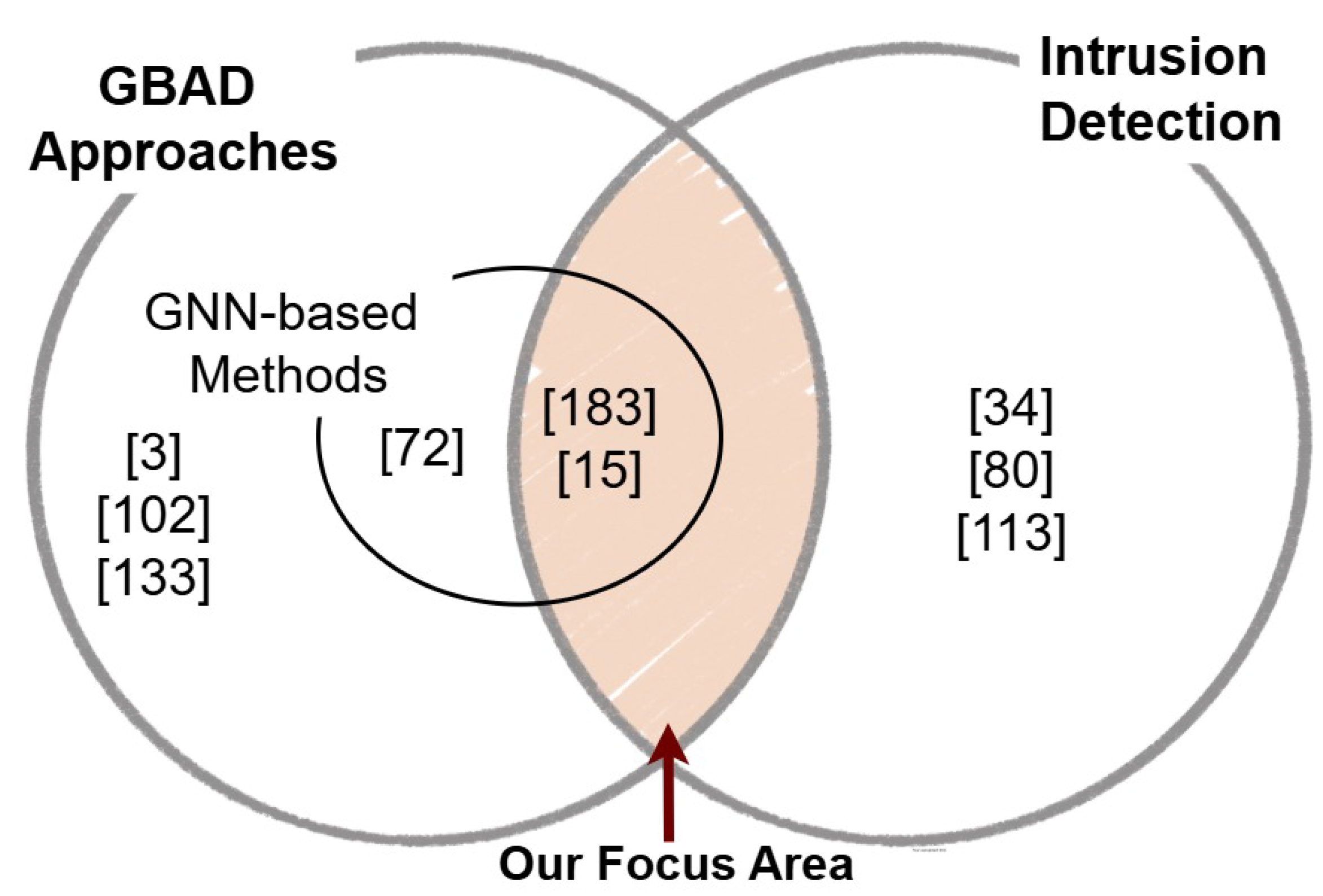
Figure 2.
Graph-based Anomaly Detection Methodology. This figure illustrates the main workflow of GBAD methods, including data capturing (A-B), graph construction (S-3), graph pre-processing (S-4), graph-based anomaly detection (S-5), and evaluation and post-detection analysis (S-6). The notation “S-x” refers to the corresponding section in the manuscript, and “A-x” denotes content described in Appendix x.
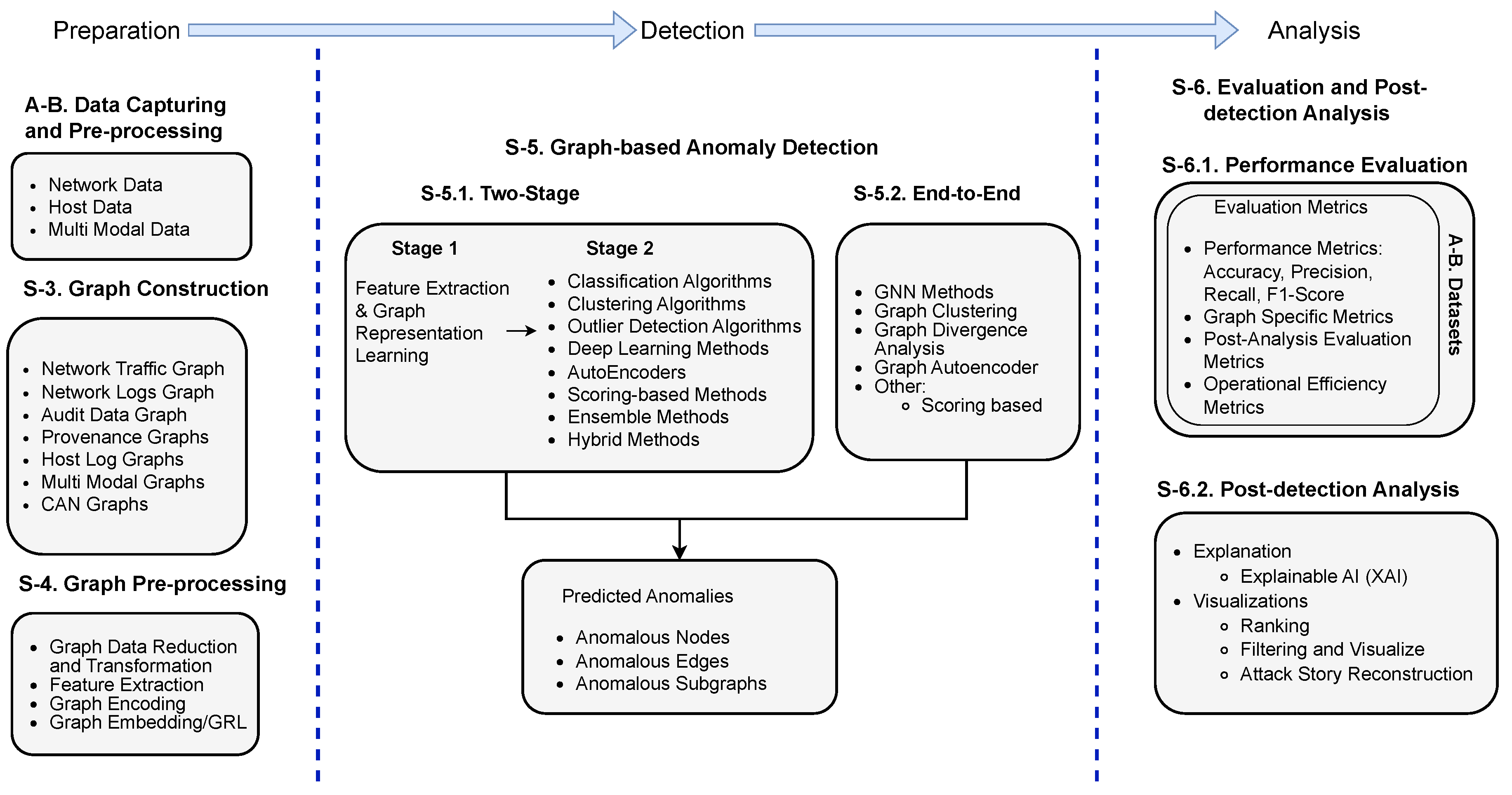
Figure 3.
Categories of graph-based anomaly detection for intrusion detection
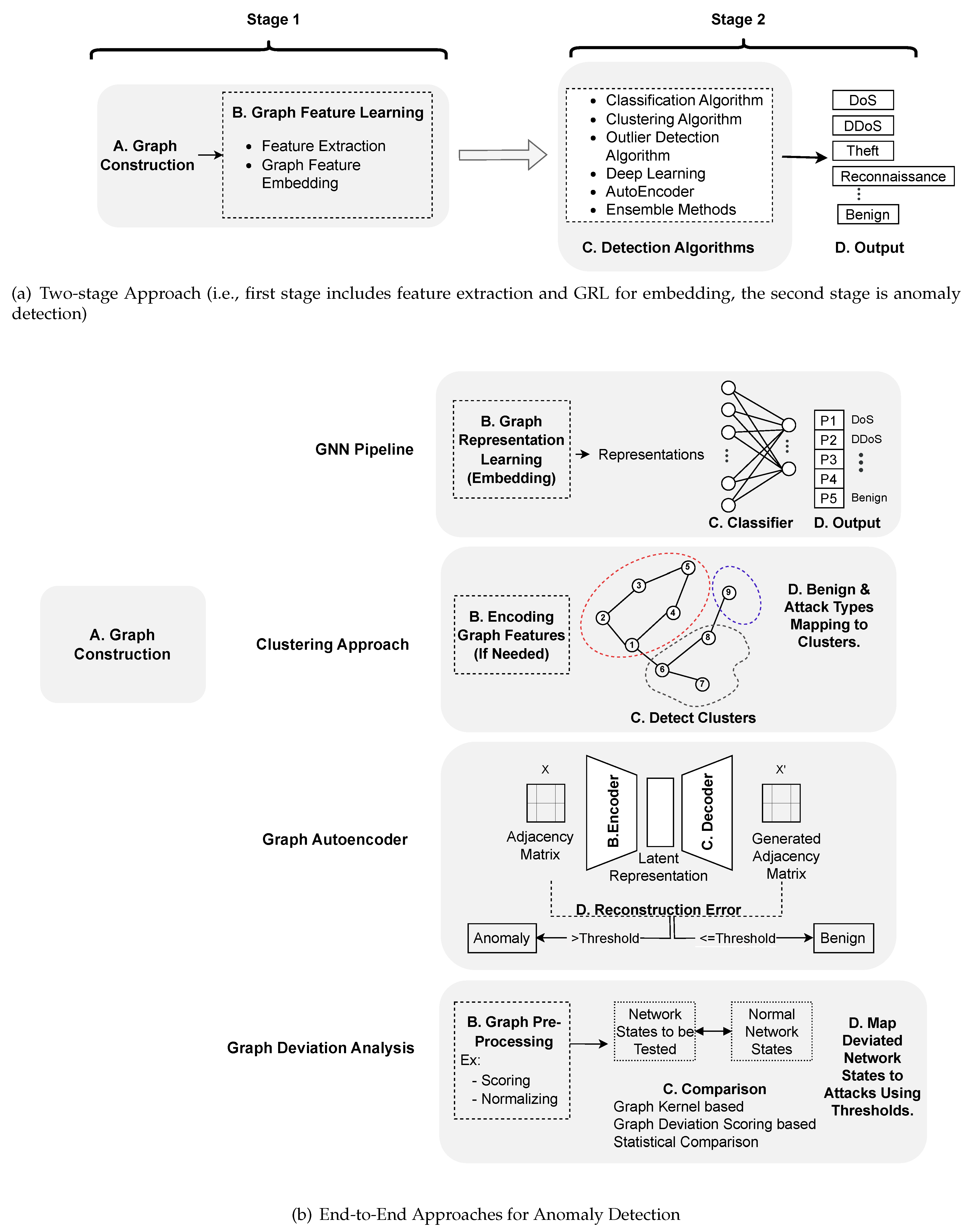
Table 1.
Summary and Comparison of Existing Surveys. The type of data represented by N-Network level data, H-Host level data, MD-Multi-dimensional data and MM-Multi-modal data. The symbols ◗ represent the survey covered a few methods under that category.
Table 1.
Summary and Comparison of Existing Surveys. The type of data represented by N-Network level data, H-Host level data, MD-Multi-dimensional data and MM-Multi-modal data. The symbols ◗ represent the survey covered a few methods under that category.
| Surveys | Year | Type of Data | Focus | Application Area | Graph-based Methods | Anomaly-based | Intrusion Detection Focus |
|---|---|---|---|---|---|---|---|
| [21] | 2020 | MD | Graph-based Anomaly Detection | Fraud Detection | ✓ | ✓ | ✗ |
| [22] | 2021 | H | Provenance Graph-based Detection | Threat Detection | ✓ | ◗ | ✗ |
| [23] | 2022 | N/A | GNN-based Anomaly Detection | Various Domains | ◗ | ✓ | ✗ |
| [24] | 2022 | N/A | Graph-based Deep Learning for Anomaly Detection | Distributed Systems | ✓ | ✓ | ✗ |
| [25] | 2023 | N, H | Graph-based Representation and Analytics | Botnet Detection | ✓ | ✓ | ✗ |
| [26] | 2023 | N, H | GNN-based Anomaly Detection | Anomaly Detection/ Intrusion Detection | ✓ | ✓ | ✓ |
| [27] | 2024 | N, H | GNN-based Anomaly Detection | Intrusion Detection | ✓ | ✓ | ✓ |
| Ours | 2025 | N, H, MM | Graph Representation Learning (GRL)-based Methods (Two-stage) & Graph-based End-to-end Methods | Anomaly Detection & Attack/Intrusion Detection | ✓ | ✓ | ✓ |
Table 2.
Summary and comparison of graph construction, detailing the data representation of nodes, edges, and attributes. Nodes and edges can be either heterogeneous (HT) or homogeneous (HM). Edges can be directed (D) or undirected (UD), and graph types include Bipartite (B), Hypergraph (HP), Spatio-Temporal Graph (ST), Snapshots (S), and Isomorphic (I).
| Graph | Node | Edges | Related Works |
|---|---|---|---|
| Network traffic graph - packet data | IP addresses and ports/network devices/hosts/data-packets/ feature of data packet with attributes of feature value [HT] | Information transmission between nodes with attributes such as # of packets or bits / # of network requests, timestamps, protocol features, domain name features [D/UD, HP] | Static graphs: [8,55,58,65,66,67,68] Dynamic graphs [ST, S]: [57,62,68,69,70,71,72] |
| Network flow graph - flow data | IP addresses with flow node feature attributes/packets with attributes such as packet length, direction/each flow as node | Traffic flow between IP addresses/connection between nodes with attributes such as similarity score of flows and flow information such as protocol, flow duration, incoming bytes, bytes per packet, Transmission Control Protocol (TCP) flags [D/UD] | Static graphs: [60,73,74,75,76,77,78] Dynamic graphs [S]: [79] |
| Network logs graph | Network events with associated attributes/hosts with attributes such as IDs, label/logline with attributes such as src and dest entity behaviors, type of behavior, time occurred/network assets | Semantic edges/network events among hosts/associations between loglines/semantic events or operations between entities [D/UD, HT, I] | Static graphs: [19,51,80,81,82] Dynamic graphs [S]: [83,84,85] |
| Provenance graph | System entities, kernel objects with attributes such as type of node [HT/HM] | System events/syscalls between entities with attributes such as edge type, timestamp [D] | Static graphs: [7,46,59,80,86,87,88,89,90] Dynamic graphs: [49,52,91,92,93,94] |
| Audit data graph | File identifiers with degree sum as attributes/login entities/users and hosts/user activity items with timestamp attribute | File transitions/login actions between entities/relationship between activity logs with timestamp attribute [D/UD, HM, HT, B] | Static graphs: [95,96] Dynamic graphs: [97] |
| Host logs graph | Log event labels with attributes formed with semantic embedding of log event | Event flows with attributes such as weight to indicate # of times events flow [D] | Static graphs: [37] |
| Control area network graphs | CAN ID/Arbitration ID with attributes of data content in CAN msg | Connect nodes based on sequence with attributes: frequency of CAN ID pair, vectorized weight [D] | Dynamic graphs: [98,99,100] |
| Multi-modal data graph | Service instances with attributes: concatenation of metric and log features | Scheduling relationship between service instances | Static graphs: [101] |
Table 3.
Graph Pre-processing Summary and Comparison
| Technique | Algorithms | Description | Related Works |
|---|---|---|---|
| Data Reduction | Pre-clustering | Pre-cluster the graph by components using high level statistics and choose cluster center. | [73] |
| Edge collation | Aggregating information from multiple edges in a graph and form a collated network. | [51,90] | |
| Sampling | Selecting a representative subset of nodes and/or edges from a large graph. | [20,89] | |
| Hoffman-based Data Adjustment | Reducing graph size by merging similar feature values and applying lossless compression. | [67] | |
| Data Transformation | Generate histogram | Build in-memory histogram runtime from streaming provenance graph. | [49] |
| Transform to line graph | Transformed to a line graph representation by changing nodes into edges vice-versa. | [74,78] | |
| Adaptive graph augmentation | Generates two structurally perturbed views to create positive and negative pairs for contrastive learning. | [74,78] | |
| Feature Extraction (FE) & Feature Optimization | Structural FE | Extract intrinsic properties of nodes and edges within the graph. | [58,100] |
| Extract behavioral features from the graph structure. | [95] | ||
| Path mining | Uses different strategies to extract meaningful paths from graphs, including DFS-based traversal, causal path selection, random walk exploration, and meta-path extraction using TF-IDS scoring. | [7,51,57,104] | |
| Sequence extraction | Extract node sequences, shingles using random walk. | [46,57,81] | |
| Graph pooling | Sort the nodes/edges of subgraph by importance score and select only the top K nodes/edges. | [63] | |
| Page Ranking | Feature generation by calculating the priority of each vertex based on its edges. | [106] | |
| Encoding | One hot encoding | Encode graph attributes and structure based on categorical features. | [19,51] |
| Word2vec | Encode sentences and phrases in graph attributes to a vector format. | [51,81,89] | |
| Hierarchical feature hashing | Encodes the node’s attribute multiple times in different levels. | [59] | |
| Vectorization | Encode causal and contextual data to row dimensional vectors, encode neighbourhood information based on poisson probability distribution. | [46] | |
| Edge feature vectorized by extracting TCP/IP layers’ bytes. | [70] | ||
| Graph Sketching | Representing states of graph using hash function to generate compact graph sketches. | [49,57,92] | |
| Spatial Temporal Node Encoding | Relative time encoding, diffusion based and distance based spatial encoding to create node embeddings by encoding global and local structure of nodes. | [20] |
Table 4.
Summary and Comparison of Graph Embedding and Representation Learning Methods, focusing on graph embedding approaches involving representation learning. The embedded features include structural and temporal attributes: N - node features, E - edge features, G - graph/subgraph features, NT - node features with temporal attributes, and ET - edge features with temporal attributes.
| Embedding Method | Algorithm | Embedded Features | Key Operations | Related Works |
|---|---|---|---|---|
| Lookup Embedding | N/A | N, E | Assigns each unique node or edge label a fixed d-dimensional vector through direct indexing in a predefined embedding matrix. | [90] |
| Distribution-based | N/A | N | Generate vector representation by minimizing the KL-divergence distance between conditional distribution and empirical distribution of nodes. | [8] |
| Random Walk-based | BiNE | N | Map two types of nodes into d-dimensional vectors. | [96] |
| CTDNE | NT | Learns node embedding using random walks while capturing timing information | [96] | |
| doc2vec and TF-IDF | G | Form sentences for graph paths using nodes and edges and then, translate the sequence of words using PV-DM model of doc2vec to convert paths to a numeric vector | [7,104] | |
| graph2vec | G | Learning whole graph representation considering set of rooted sub graphs | [52,60] | |
| Interval inclined random walk | ET | Spatial features including edge features and temporal features of a graph stream embedded as vectors | [55] | |
| GNN-based | GCN | N, E, ET, G | Learn embedding of each node and aggregates embeddings from all its neighbours | [63,67,79,86] |
| GraphSAGE | N, E | Iteratively aggregates neighbouring node information at k-hop depth and sampled to generate node/edge embeddings | [62,65,75,76,77,89] | |
| GAT | N | Aggregating both local and root neighborhood information through weighted summation | [93] | |
| Attention-based | N | Generates embeddings by weighting and aggregating graph features using attention mechanisms | [80] | |
| Multi perspective | N, G | Generated node embeddings with GNN and send those through mean pooling layer to get graph embeddings | [103] | |
| Streaming Implementation | N | Graph sketching with MPNN to embed streaming graph data | [92] | |
| Graph Autoencoder-based | GAT layers for encoder and decoder | N | Learn node embeddings by encoding and reconstructing graph features. | [90] |
| GNN-based encoder and reconstruction decoder | N | Combines message-passing encoders with a decoder based on Neighborhood Wasserstein Reconstruction to capture and reconstruct both structural and feature-based neighborhood information. | [88] | |
| Spatial-nonspatial Embedding | MLP, GCN, GAT | N | Non-spatial data embed to lower space with MLP and spatial information with GCN and GAT | [74] |
| Advanced Embedding Methods | Graph Structure Learning | N | Learn the relationships between characteristic dimension | [12] |
| Event-property composite model | N | A novel NRL learning event- and property-level representations in a property graph using MARINE and GNN models. | [109] | |
| Infograph | G | Learn graph embedding by maximizing mutual information between normal paths and normal network activity patterns | [51] |
Table 5.
Summary and Comparison of Two-Stage Graph-Based Anomaly Detection (GBAD) Models and Algorithms. The notations represent ✓ for real-time detection, ✗ for non-real-time detection and ◗ for near real-time detection. Supervision represents S: Supervised, US: Unsupervised, SS: Semi-Supervised, SfS: Self-Supervised.
| AD Model | Algorithm | Supervision | Real-time | Inputs | Type of Graph Anomaly | Related Works |
|---|---|---|---|---|---|---|
| ML Classification | Random Forest | US S S |
✗ ◗ ✓ |
Node embeddings Subgraph embeddings Structural and temporal embeddings |
Node Subgraph Node |
[8] [60] [55] |
| Isolation Forest | US | ✗ | Encoded features, Node embeddings | Node | [88] | |
| XGBoost | SS | ◗ | Encoded features, Node embeddings | Node | [89] | |
| OCSVM and Isolation Forest | US | ✗ | Behavioral features | Node | [95] | |
| Catboost Classifier | S | ✗ | Edge embeddings | Edge | [77] | |
| Logistic Regression | S | ✓ | Structural and temporal embeddings | Path | [96] | |
| Clustering | K-Means | SfS | ✗ | Node embeddings | Node | [93] |
| K-medoid | US | ✓ | Graph sketches | Subgraph | [49] | |
| Customized distance based | US | ✗ | Graph embeddings | Node | [81] | |
| Outlier Detection | K-nearest neighbours (KNN) | US | ✗ | Node embeddings | Node | [90] |
| Copula based Outlier Detector (COPOD) | US | ✗ | Node embeddings | Path | [51] | |
| Robust Random Cut Forests (RRCF) | US | ✓ | Graph sketch vector | Node | [57] | |
| Local Outlier Factor (LOF) | US | ✗ | Path embeddings | Path | [7] | |
| Deep Learning | Neural Networks: | |||||
| - Recurrent CNN | US | ◗ | Subgraph embeddings | Subgraph | [52] | |
| - LSTM + BNN | S | ✗ | Vectorized graph data | Subgraph | [46] | |
| - MLP | S | ✓ | Node embeddings | Node | [62] | |
| - Dynamic GNN | SS | ✓ | Spatial & temporal embeddings | Node | [79] | |
| Generative Adversarial Network (GAN) | US US |
✓ ✓ |
Node embeddings Edge encodings |
Subgraph Edge |
[92] [20] |
|
| Transformer-based Networks | S | ✓ | Subgraph embeddings | Subgraph, Path | [104] | |
| Autoencoder | S US US US SS |
✗ ✗ ✗ ✗ ✓ |
Learned relations Encoded graph data Structural features Graph embeddings Generated features |
Node Edge Node Graph Node |
[12] [19] [58] [86] [106] |
|
| Scoring-based Methods | TF-IGF Approximation | US | ◗ | Encoded graph features | Edge | [114] |
| SEDANSCORER | US | ◗ | Sampled Subgraphs | Edge | [129] | |
| Ensemble Methods | LightGBM Classification + Clustering | S | ✗ | Node embeddings | Node | [67] |
| Hybrid Methods | Autoencoder + Negative Sampling | US | ✗ | Node & graph embeddings | Node, Edge | [80] |
| Deep SVDD | US | ✓ | Node & graph embeddings | Subgraph | [103] |
Table 6.
Summary and Comparison of End-to-End Graph-Based Anomaly Detection (GBAD) Models and Model Architectures. The notations represent ✓ for real-time detection, ✗ for non-real-time detection and ◗ for near real-time detection. Supervision represents S: Supervised, US: Unsupervised, SS: Semi-Supervised, SfS: Self-Supervised.
| Anomaly Detection Model | Model Architecture | Description | Inputs | Supervision | Real-time | Type of Graph Anomaly | Related Works |
|---|---|---|---|---|---|---|---|
| GNN | GCN | Aggregate features from neighboring nodes to update representations | Vectorized Node & Edge Attributes | S | ✓ | Node | [68,83] |
| GCN with One Class Classifier | GCN is used to learn graph representations, followed by one-class classifiers (e.g., SVM, SVDD) to detect anomalies | CAN Graph Multi-modal Data Graph Host Logs Graph |
S S US |
✓ ✓ ✗ |
Node Node Node |
[98] [108] [37] |
|
| GraphSAGE-based | Learn representation of nodes/edges by sampling a fixed size neighborhood of each and aggregate information from those neighbors | Network Flow Graph Network Traffic Graph Provenance Graph |
S S S |
✗ ✗ ✗ |
Edge Edge Node | [75] [65] [94] |
|
| GAT-based | Learn the weights of each node in neighbors during message passing | Vectorized Nodes Line Graph Network Traffic Graph |
S S S |
◗ ✗ ◗ |
Node Node Node |
[91] [74] [71] |
|
| GCN combined with GAT | Two GCN layer for learning time features and distance features followed by GAT layer to capture the importance of activity logs | Audit Data Graph | S | ✗ | Node | [97] | |
| GCN with Graph Contrastive Learning | GCN-based encoder learns node embeddings using contrastive and classification losses, with federated training | Network Flow Graph | SS | ✗ | Node | [78] | |
| Knowledge-enabled GNN | Integrate structured domain knowledge into the GNN learning process | Network Logs Graph | S | ✗ | Edge | [82] | |
| GNN with Temporal Models (GRU, TGN, LSTM) | Enabling dynamic representation learning and anomaly detection by processing time-varying features and updating node or edge embeddings across timestamps | Dynamic Graph Dynamic Graph Dynamic Graph Multi-modal Data Graph |
S S S US |
✗ ✓ ✗ ✓ |
Edge Edge Node Node |
[63] [84] [59] [107] |
|
| Clustering | Vertex Cover Optimization | Pre-cluster edges to detect critical vertices and identify abnormal edges through Z3 SMT solver and clustering loss analysis | Network Flow Graph | US | ✓ | Edge | [73] |
| Micro-clustering-based | Running parallel instances of micro-cluster detection with different attributes and anomaly score for each calculated using the MIDAS algorithm | Dynamic Graph | US | ✓ | Subgraph | [85] | |
| Evolutionary Graph Clustering | Extract community evolution events and use those results for detecting anomalous evolutionary paths | Dynamic Graph | US | ✗ | Event | [64] | |
| Graph Divergence Analysis | Graph Kernel-based | Calculate graph divergence using WL Kernel and detect using a dynamic threshold (Improved EWMA) | Network Traffic Graph | US | ✓ | Graph | [69] |
| Graph Divergence Scoring | Compare subgraph structures, forecast expected behaviors to compute deviation scores, and flag anomalies when exceed a threshold. | CAN Graph Forecasted and observed node data |
S US |
✓ ✗ |
SubgraphNode | [99] [12] |
|
| Statistical Comparison | Uses chi-squared test to compare graph features between normal and test populations | CAN Graph | SS | ◗ | Subgraph | [100] | |
| Statistical Graph Analysis + Time Series Analysis | Using ERGM to perform statistical analysis of Network Topology Graphs and ARMA model to perform time series analysis of coefficients | Network Traffic Graph | US | ✗ | Subgraph | [66] | |
| Graph Autoencoders | Graph Transformer-based | Transformer encoder and DNN decoder reconstruct edge attributes, with anomalies detected via reconstruction and ML model | Network Traffic Graph | US | ◗ | Edge | [70] |
| Temporal Graph Transformer | Adversarial autoencoder with graph and temporal attention | Network Traffic Graph | US | ✗ | Graph | [72] | |
| Multi-Modal Temporal Graph Transformer | Transformer-based model with spatial, temporal, & cross-modal attention; detects anomalies from multi-modal graph reconstruction | Microservice Twin Graph | SS | ✓ | Graph | [101] | |
| Others | Scoring/Weighting-based | Weights graph edges using anomaly scores from coarse logs, prunes low-weight edges, and extracts attack paths from the refined graph | Provenance Graph | S | ✗ | Subgraph | [87] |
Table 7.
Application-Oriented Comparison of Two-Stage vs. End-to-End Graph-Based Anomaly Detection (GBAD) Approaches
Table 7.
Application-Oriented Comparison of Two-Stage vs. End-to-End Graph-Based Anomaly Detection (GBAD) Approaches
| Aspect | Two-stage Approach | End-to-end Approach |
|---|---|---|
| Flexibility | High - can swap components | Low- unified architecture |
| Supervision Requirement | Flexible - support supervised, sem- and unsupervised learning | Often supervised - especially in GNN based models |
| Real-time Capability | Moderate - operates mainly in batch model and limited real time use | Better for real-time and streaming |
| Intepretability | Better - clear pipeline | Limited - black box |
| Computational Complexity and Scalability | Lower - simpler components and stage-wise optimization | Higher - complex models like GNN |
| Anomaly Granularity | Multi-level - detects node, edge, subgraph, and graph-level anomalies | Specialized - GNNs mostly focus on node/edge, non-GNNs on graph/subgraph |
| Best Use Case needed | Forensic or exploratory analysis where interpretability and flexibility are key | Real-time or adaptive intrusion detection emphasizing automation and speed |
Table 8.
Summary and Comparison of Datasets across GBAD Studies
| Type | Dataset | Detected Attacks/Anomalies | Description | Related Works |
|---|---|---|---|---|
| Network Datasets | CICIDS [143] | DoS, DDoS, Web Attack, Infiltration, Port scan, Botnet | Network traffic data provided in pcap and CSV formats, with extracted flow features | [19,60,70,74,76,77,78] |
| UNSW-NB15 [144] | Exploits, Reconnaissance, DoS, Generic, Shellcode, Fuzzers, Worms, Backdoors, Analysis | Consists of real benign and simulated attack activity traffic data logs collected from simulation environments | [51,65,72,76,77,85,92] | |
| Network Traffic | DDoS, CMP, UDP/TCP SYN Flood, Botnet attacks; IoT: ARP spoofing, Ping of Death, Smurf, DoS | Multiple datasets including DDoS with varying attack rates [145], CTU-13 Botnet [146], Kyoto 2006+ datasets [147], TOR-nonTOR [148], SUEE8 [149], smart home IoT traffic [57] | [57,69,83,85,109] | |
| Malware Traffic | Malware attacks | AndMal2019 [150] (malicious apps in smart devices), EncMal2021 [55] (user-submitted malicious executables) | [55] | |
| AWID-CLS-R [151] | Flooding, Impersonation, and Injection | Open-source dataset with MAC-layer traces of benign and malicious activities in 802.11 WLAN traffic. | [72] | |
| CERT [152] | Insider threats | Network logs for 100B+ behaviors of 4000 users | [81,84,97] | |
| IoT | Malware, Botnets, DoS, DDoS, Scanning, Password cracking, Ransomware, Injection, MITM, XSS, Backdoor | Traffic data, operational logs, and telemetry data collected from an IoT environment. Some IoT datasets are IoT-23, MedBIoT, Bot-IoT [153], ToN-IoT, NF-Bot-IoT, NF-ToN-IoT [154], IOST [155], ACI-IoT-2023 [156] and CICIoT2023 [157] | [12,58,62,67,68,70,71,74,75,78,79] | |
| Real-world Generated | APT, Trojan, Phishing, DNS Exfiltration, Brute force, Encrypted flooding/malicious traffic | Normal and network-level events were collected from an enterprise network, and an attack testbed generated multiple attack types | [63,66,73] | |
| CAN | DoS, Fuzzy, Suspension, Replay, Spoofing, Impersonation | Consist of CAN messages collected from an in-vehicular network. Some CAN datasets are CAN signal datasets [158] and OTIDS [159] which is a real vehicle datasets from HCRL | [98,100,106] | |
| Host Datasets | WUIL [160] | Data breaching | File system access dataset including 3050 normal and 222 attack samples | [95] |
| DARPA | APT, Phishing, Dictionary attacks, FTP-write, Port scan | IDS data with full packet captures, featuring the 1999 set, OpTC dataset for APT activities, and Engagement datasets (E3 and E5) simulating real-world APT scenarios | [46,52,59,85,89,90,91,92,93,106] | |
| ATLAS [161] | 10 types of APT attacks | Labeled dataset of logs collected from a real-world system which consists of 20,088 entities and 249k events per scenario | [52,93] | |
| StreamSpot [162] | Drive-by download attack | Consists of 500 benign graphs for 5 scenarios and 100 attack graphs for 1 attack scenario generated from data collected on Linux machines | [52,80,86,89,90,92,93,94,162] | |
| LANL [163] | APT attacks | Contains 1,648,275,307 events comprising benign events (authentication, network flow, DNS lookup) and attack events | [80,82,84,96] | |
| Unicorn [49] | APT attacks like malware downloads, remote code execution, and command injection | System provenance dataset collected using CamFlow, capturing system-level activities over three days with 125 benign graphs and 25 attack graphs. SC-1 and SC-2 versions available | [89,90,94] | |
| Production EDR [52] | APT attacks | Includes EDR logs from 18K endpoints and 59K extracted graphs | [52] | |
| Generated datasets | Attacks for enterprise systems such as reconnaissance, credential access, privilege escalation, file and system manipulation etc. | System logs containing simulated attack logs for 16 attack types | [87,103] | |
| Multi-modal Datasets | DeepTraLog [164] | Service fault anomalies | Consists of 132,485 traces and 7.7M log messages, where 17% of those are anomalous | [108] |
| BETH [165] | Unusual/malicious activities | Kernel-level process logs and network traffic | [88] | |
| MSDS [166] | Anomalies | Consist of traces, logs, and metrics from an OpenStack-distributed system | [101] | |
| AIOps-Challenge | Service, Pod and Node anomalies | Instance metrics and logs for 40 services on 6 servers in a microservice-based system | [101] | |
| TraceRCA and TT-ARM [167] | Anomalies | Datasets with traces and metrics from microservice-based systems | [107] |
Table 9.
Post-Detection Analysis Summary and Comparison
| Methods | Description | Target Users | Related Works | |
|---|---|---|---|---|
| Model Explanations | Explainable AI (XAI) | PGExplainer for local and global explanations. | Security analyst,Researchers | [77] |
| Investigate Anomalous Results | Ranking | Rank the RSGs based on co-occurrence probability and select key indicators. | Security analysts | [52] |
| Filtering and Visualize | Subset of important nodes filter using LPR algorithm and presented in an anomalous log graph. | Security analysts | [37] | |
| For the detected anomalous graph, apply graph reduction techniques and community discovery algorithm to construct attack summary graphs and benign graphs. | System admins | [59] | ||
| Attack Story Reconstruction | Used the activation (output) of layers to get the training event trace similar to the input that generated the malicious prediction output. | Cyber defense team | [46] |
Disclaimer/Publisher’s Note: The statements, opinions and data contained in all publications are solely those of the individual author(s) and contributor(s) and not of MDPI and/or the editor(s). MDPI and/or the editor(s) disclaim responsibility for any injury to people or property resulting from any ideas, methods, instructions or products referred to in the content. |
© 2026 by the authors. Licensee MDPI, Basel, Switzerland. This article is an open access article distributed under the terms and conditions of the Creative Commons Attribution (CC BY) license (http://creativecommons.org/licenses/by/4.0/).
Copyright: This open access article is published under a Creative Commons CC BY 4.0 license, which permit the free download, distribution, and reuse, provided that the author and preprint are cited in any reuse.


