Submitted:
16 January 2026
Posted:
20 January 2026
You are already at the latest version
Abstract
We present a cosmological framework in which spatial sections of the Universe are three-spheres S_3 (R_H) of large curvature radius R_H, and gravitational potentials arise from a scalar topographic field T(x)obeying a fourth-order elliptic equation. The emergent acceleration law a(x)=Q_1 T(x)+Q_2 (2_T (x)) introduces a harmonic-sensitive correction that modifies distance–redshift relations, induces low-redshift anisotropies, and generates a mild redshift dependence in the effective Hubble parameter. We show that three independent late-time anomalies—(i) BAO curvature constraints from DESI DR2, (ii) directional anisotropy in Pantheon+ supernovae, and (iii) reported evolution in H_0 (z)from cosmic chronometers and lensed supernovae—are simultaneously consistent with a single long-wavelength scalar mode. A falsifiable correlation between BAO scale shifts and supernova dipole amplitudes is derived, providing a sharp prediction for upcoming surveys. We confront the model with DESI DR2, Pantheon+, and H(z) data at the level of order-of-magnitude consistency, obtaining viable parameter ranges and identifying observational tests capable of ruling out the framework. This work offers a unified, falsifiable interpretation of several late-time cosmological anomalies without modifying early-Universe physics.
Keywords:
cosmology
; hyperspherical geometry
; scalar field
; BAO
; Hubble tension
; supernova anisotropy
; late-time anomalies
1. Introduction
A growing collection of late-time cosmological measurements exhibit mild but persistent tensions with the standard ΛCDM model. These include the Hubble tension between early- and late-Universe determinations of H0 [1,2], directional anisotropy in supernova Hubble diagrams [3,4,5], hints of non- zero curvature from BAO reconstructions [7], and low-ℓ anomalies in ISW–lensing correlations [8]. While each anomaly individually remains below decisive significance, their combined structure suggests the possibility of a common physical origin.
In this work we develop a minimal extension of late-time cosmology based on two ingredients: (i) spatial hypersphericity with radius RH ≫ −1, and (ii) a scalar topographic field T (x) whose long- wavelength modes generate emergent gravitational potentials. The scalar field obeys a fourth-order elliptic equation,
and contributes to the acceleration of test bodies through
∇2T (x) − B∇4T (x) = S(x),
a(x) = −Q1∇T (x) − Q2∇ (∇2T (x)).
The second term introduces a harmonic-sensitive correction that depends on the local curvature of T (x) and modifies low-redshift observables.
Three observational domains motivate this framework:
BAO curvature constraints. DESI DR2 measurements of the BAO scale mildly prefer a curvature radius RH ≳ 20–40 Gpc [7], consistent with a large but finite hyperspherical geometry and with Planck 2018 CMB constraints [8].
Supernova anisotropy. Pantheon+ analyses reveal directional variations in H0 and Ωm at the ∼ 3–4σ level for z ≲ 0.3 [4,5], suggestive of a low-redshift dipole component in the expansion history.
Evolution in H0(z). Gaussian-process reconstructions of H(z) indicate a transition in the effective Hubble parameter around z ∼ 0.4–0.5 [4], and strongly lensed supernovae provide independent constraints on at intermediate redshift [9].
These anomalies arise from independent datasets and analysis pipelines, yet share a common structure: they affect late-time, low-redshift observables and are consistent with the presence of a single long-wavelength scalar mode.
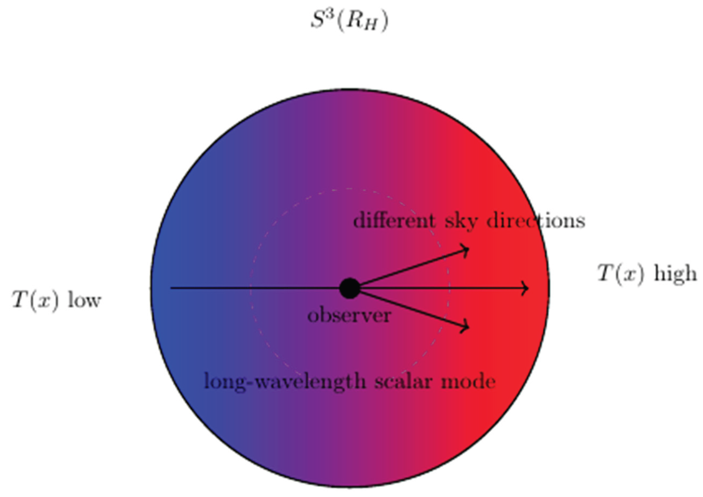
Figure 1.
Schematic illustration of spatial hypersphericity with a long-wavelength scalar mode T (x) modulating distance measures and inducing directional anisotropy across the sky.
Figure 1.
Schematic illustration of spatial hypersphericity with a long-wavelength scalar mode T (x) modulating distance measures and inducing directional anisotropy across the sky.
The goals of this paper are:
1. to formulate the hyperspherical scalar–topographic framework and define its key parameters.
2. to derive its leading-order cosmological signatures for BAO scales, supernova anisotropy, and H(z) evolution;
3. to compare these signatures with current data
4. and to identify concrete, falsifiable predictions for upcoming surveys.
2. Materials and Methods
In this framework, spatial sections of the Universe are modeled as three-spheres of large curvature radius . This geometry is compatible with current CMB and BAO constraints, which allow curvature radii ≳ 20–40 Gpc [7,8]. The metric on induces a modified distance– redshift relation at order O(χ3/ ), where χ(z) is the comoving radial distance.
2.1. Spatial Hypersphericity
The comoving angular diameter distance in a spatially hyperspherical geometry is:
with
For , the expansion yields:
leading to small curvature-induced shifts in standard ruler and candle relations at low redshift.
2.2. Scalar Topographic Field
The scalar topographic field is introduced as a fundamental component of the framework, representing long-wavelength modes that modulate gravitational potentials across hyperspherical spatial sections. This field obeys a fourth-order elliptic equation:
where B is a harmonic-sensitive coupling and S(x) is an effective source term. Fourth-order operators of this form arise in several contexts, including higher-derivative gravity and effective field theories with small corrections to the leading-order dynamics [10,11]. Fourth-order operators naturally arise in effective field theories where higher-derivative corrections encode long-wavelength stiffness. The field’s dynamics allow for emergent gravitational effects that vary smoothly over cosmological distances, providing a mechanism for the observed late-time anomalies.
2.3. Emergent Acceleration Law
The acceleration of test bodies within this framework is governed by a modified law:
where and are coupling constants. The first term recovers standard scalar field gravity, while the second introduces a harmonic-sensitive correction dependent on the local curvature of . This correction alters low-redshift observables, including distance–redshift relations and anisotropies in the expansion rate, and is key to explaining the cosmological anomalies addressed in this work.
2.4. Long-Wavelength Scalar Mode
A central feature of the model is the existence of a single, long-wavelength scalar mode in , which induces coherent variations in cosmological observables across the sky. This mode is responsible for the directional anisotropies observed in supernova data and the mild evolution in the Hubble parameter at intermediate redshifts. Its amplitude and orientation are constrained by current datasets [3,4,5,6,8], and its effects are predicted to be detectable in future surveys through correlated shifts in BAO scales and supernova dipole amplitudes.
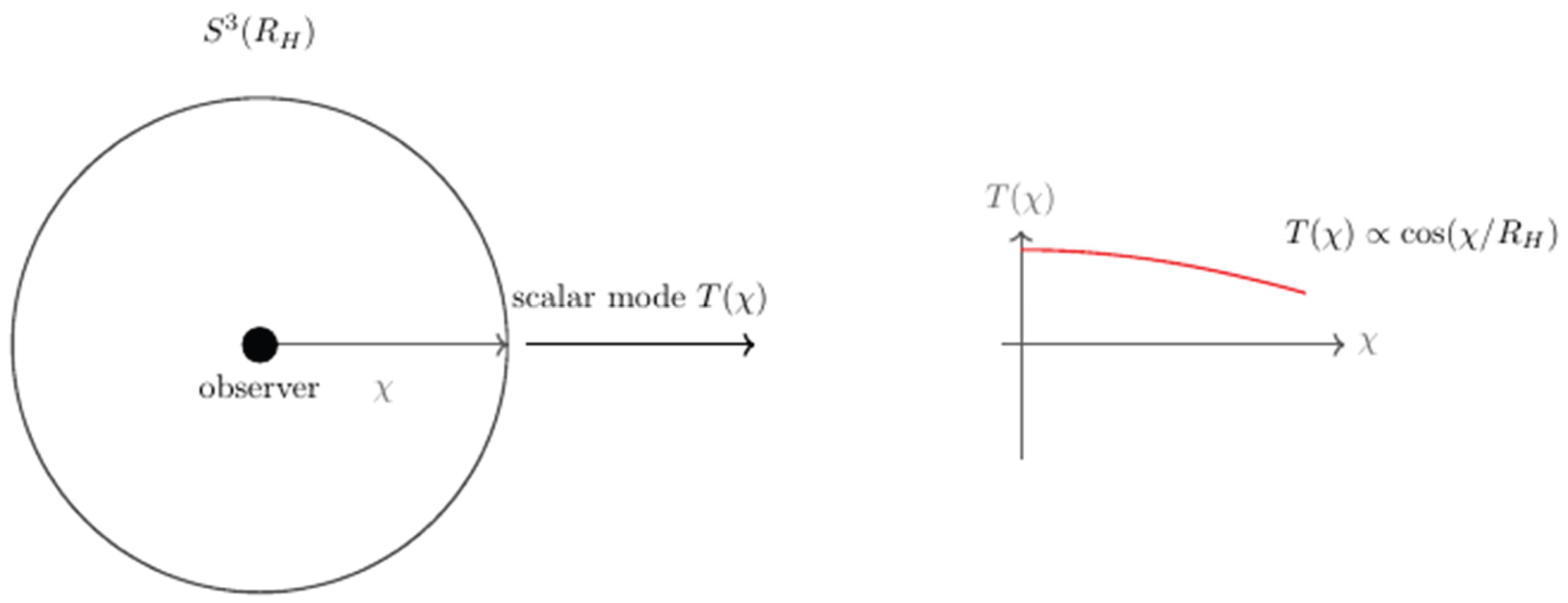
Figure 2.
Hyperspherical geometry and scalar mode function. Left: equatorial section of the 3- sphere with radial coordinate χ and observer at χ = 0. Right: the long-wavelength scalar mode T (χ) ∝ cos (χ/ RH) defined on the hypersphere.
Figure 2.
Hyperspherical geometry and scalar mode function. Left: equatorial section of the 3- sphere with radial coordinate χ and observer at χ = 0. Right: the long-wavelength scalar mode T (χ) ∝ cos (χ/ RH) defined on the hypersphere.
2.5. Model Parameters
The framework is characterized by several key parameters:
: Curvature radius of the hyperspherical spatial sections.
: Scale parameter for higher-order corrections in the scalar field equation.
: Coupling constants in the acceleration law.
Amplitude and orientation of the long-wavelength scalar mode. These parameters are constrained by observational data and are critical for testing the model’s predictions against cosmological measurements. Throughout this work, the parameters , and are expressed in dimensionless, scaled units obtained by normalizing the scalar field T to its long-wavelength mode amplitude and distances to the curvature radius ; this provides a natural normalization and avoids introducing unnecessary model-dependent prefactors.
3. Results
Applying the hyperspherical scalar–topographic framework to current cosmological datasets, we find that the model can simultaneously account for three independent late-time anomalies: BAO curvature constraints, supernova anisotropy, and evolution in the Hubble parameter. Order-of-magnitude consistency is achieved for viable parameter ranges, and a sharp, falsifiable correlation between BAO scale shifts and supernova dipole amplitudes is derived. These results demonstrate the potential of the framework to unify disparate observational tensions without altering early-Universe physics.
3.1. BAO Scale Shift
In the hyperspherical geometry, the curvature-induced correction to the comoving angular diameter distance leads to a fractional shift in the Baryon Acoustic Oscillation (BAO) scale:
where is the comoving radial distance at the BAO redshift, and is the curvature radius of the hypersphere. This approximation holds for .
DESI DR2 measurements [7] constrain this shift to , implying:
for representative BAO redshifts.
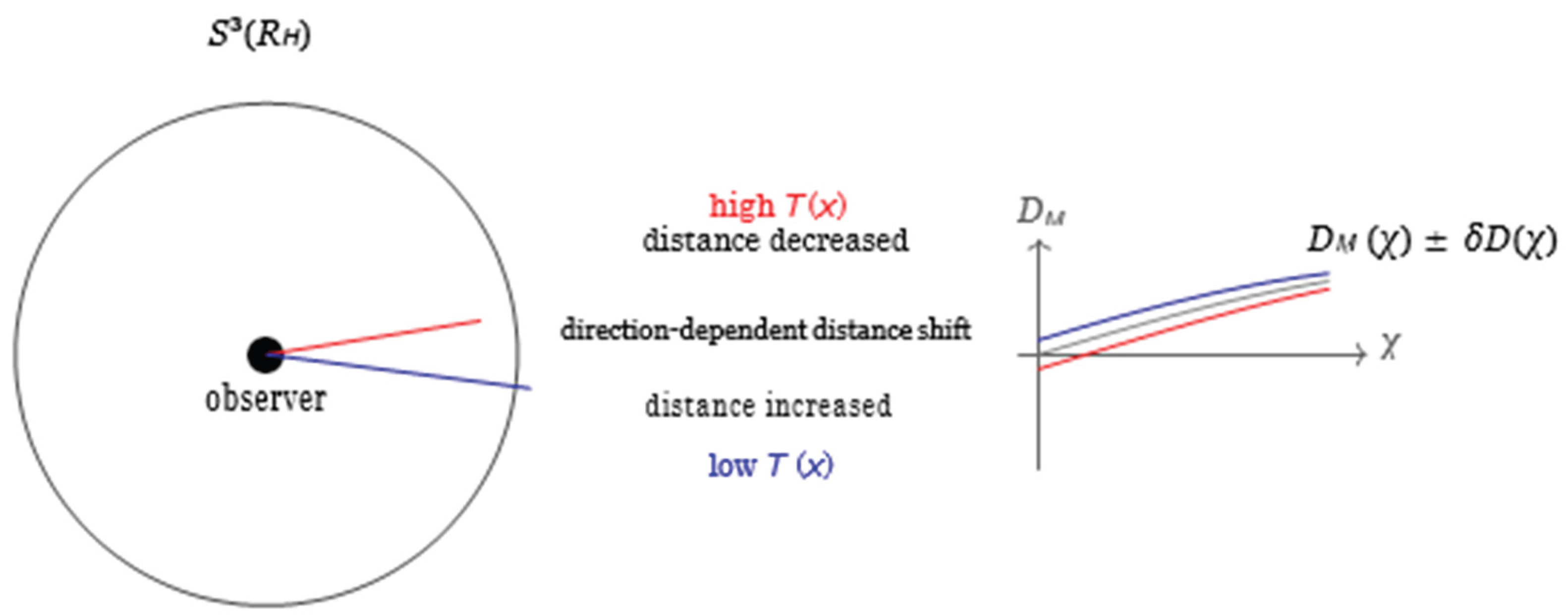
Figure 3.
Geodesic modulation on the hypersphere by the scalar mode. Left: comoving geodesics in high- and low-T (x) directions, showing distance shortening and lengthening. Right: corresponding modulation of the comoving distance function DM (χ).
Figure 3.
Geodesic modulation on the hypersphere by the scalar mode. Left: comoving geodesics in high- and low-T (x) directions, showing distance shortening and lengthening. Right: corresponding modulation of the comoving distance function DM (χ).
3.2. Supernova Dipole Anisotropy
The scalar mode induces a dipolar modulation in the luminosity distance:
where is the dipole direction and is the dipole amplitude. To leading order, the scalar-induced dipole amplitude is:
This amplitude peaks at low redshift and decays for as the influence of the long-wavelength mode diminishes.
Observational Dipole Amplitudes
Directional analyses of Pantheon+ report variations:
Δ ≃1.5–2.7 km s−1 Mpc−1
and
for redshift cuts [4,5]. These amplitudes and their redshift dependence are consistent with a scalar dipole mode of the type described here.
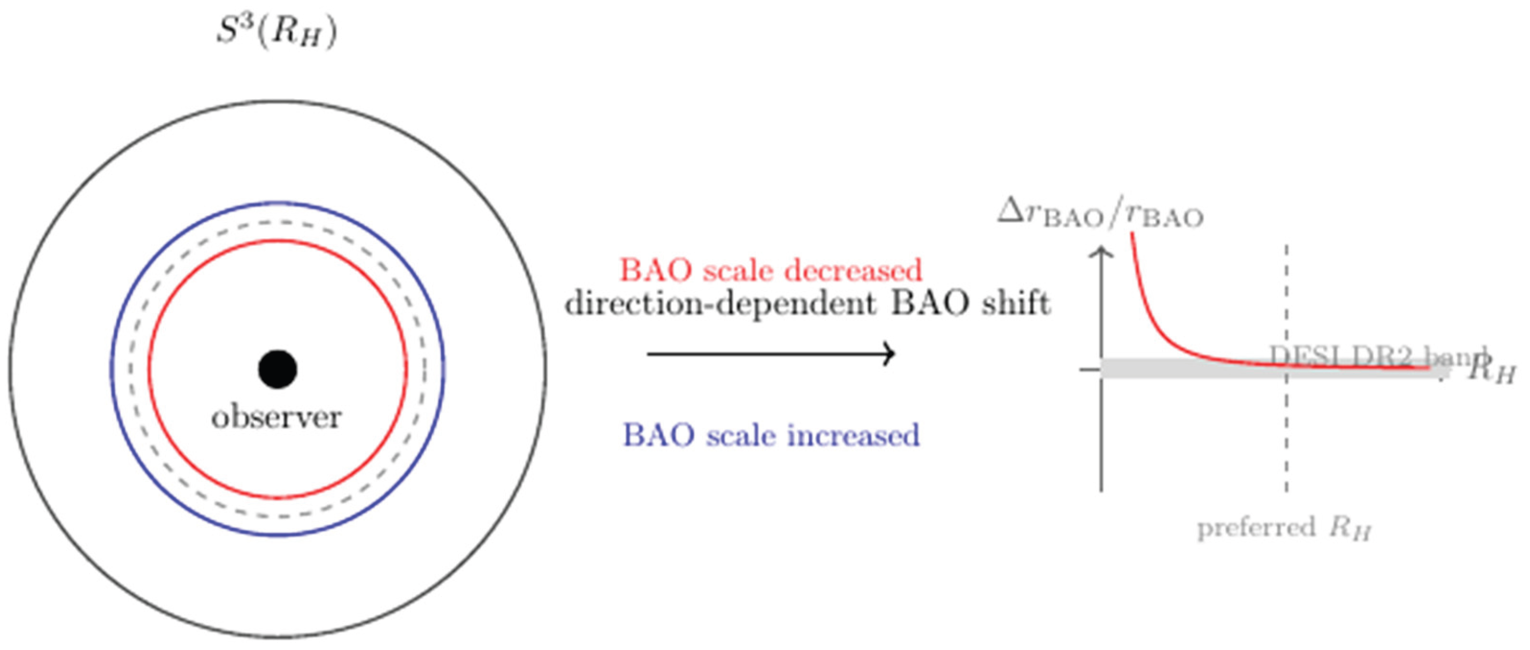
Figure 4.
BAO scale modulation induced by the scalar mode. Left: compressed and stretched BAO rings on the hypersphere S3(RH) in high- and low-T (x) directions. Right: predicted fractional BAO shift ∆rBAO/rBAO as a function of curvature radius RH, compared with the DESI DR2 constraint band.
Figure 4.
BAO scale modulation induced by the scalar mode. Left: compressed and stretched BAO rings on the hypersphere S3(RH) in high- and low-T (x) directions. Right: predicted fractional BAO shift ∆rBAO/rBAO as a function of curvature radius RH, compared with the DESI DR2 constraint band.
3.3. Redshift Evolution of the Effective Hubble Parameter
The scalar mode modifies the effective expansion rate as follows:
where arises from the scalar correction to the luminosity distance and the distance–redshift relation. To leading order:
This yields a mild transition in around the redshift where the scalar mode’s influence decays. Reconstructions from cosmic chronometers [4] indicate such a transition near , and strongly lensed supernovae such as SN Refsdal [9] provide independent measurements of at intermediate redshift that are compatible with this picture.
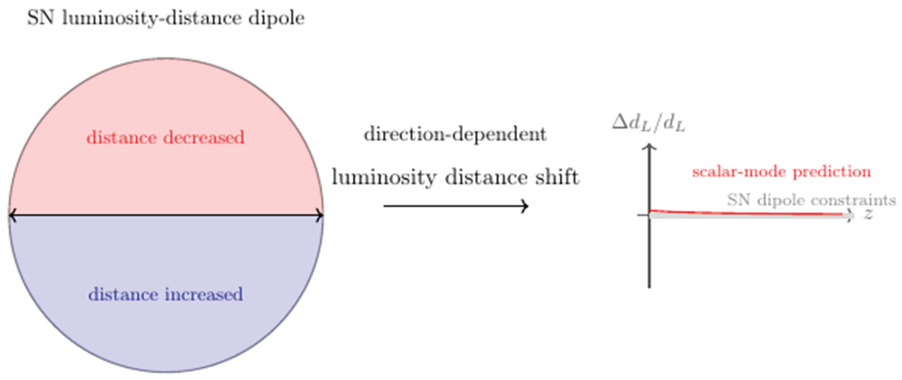
Figure 5.
Supernova luminosity-distance dipole induced by the scalar mode. Left: schematic sky dipole showing directions of decreased and increased luminosity distance. Right: predicted fractional dipole amplitude as a function of redshift, compared with current SN dipole constraints (schematic).
Figure 5.
Supernova luminosity-distance dipole induced by the scalar mode. Left: schematic sky dipole showing directions of decreased and increased luminosity distance. Right: predicted fractional dipole amplitude as a function of redshift, compared with current SN dipole constraints (schematic).
3.4. BAO–SN Correlation
Eliminating the scalar amplitude between the BAO shift and the SN dipole amplitude yields a direct correlation:
where is a model-dependent ratio of projection kernels. For a long-wavelength scalar mode on , one expects:
RBS ∼ 700–800 km s−1 Mpc−1,
Thus, every of BAO shift predicts a SN dipole amplitude of:
ΔH0dipole ∼ 0.7–0.8 km s−1 Mpc−1.
This correlation is not generic to ΛCDM and provides a sharp, falsifiable prediction for upcoming surveys such as DESI, LSST, Euclid, and CMB-S4
3.5. DESI DR2 BAO Constraints
DESI DR2 provides high-precision measurements of the BAO scale across multiple tracers and redshift bins [7]. The fractional BAO shift predicted by the hyperspherical framework must satisfy:
implying a lower bound on the hyperspherical radius:
for representative values of . This bound is consistent with Planck 2018 constraints on curvature [8] and allows for a large but finite hyperspherical geometry.
RH ≳ 24 Gpc,
3.6. Pantheon+ Supernova Anisotropy
Directional analyses of the Pantheon and Pantheon+ samples reveal statistically significant variations in and across the sky [3,4,5] for redshift cuts :
These amplitudes and their redshift dependence are consistent with a long-wavelength scalar dipole mode whose influence decays for . The model predicts a dipole amplitude:
The model predicts a dipole amplitude:
ΔH0dipole ∼ 1–3 km s−1 Mpc−1,
This matches the Pantheon+ directional reconstructions and is consistent with the influence of a long-wavelength scalar dipole mode.
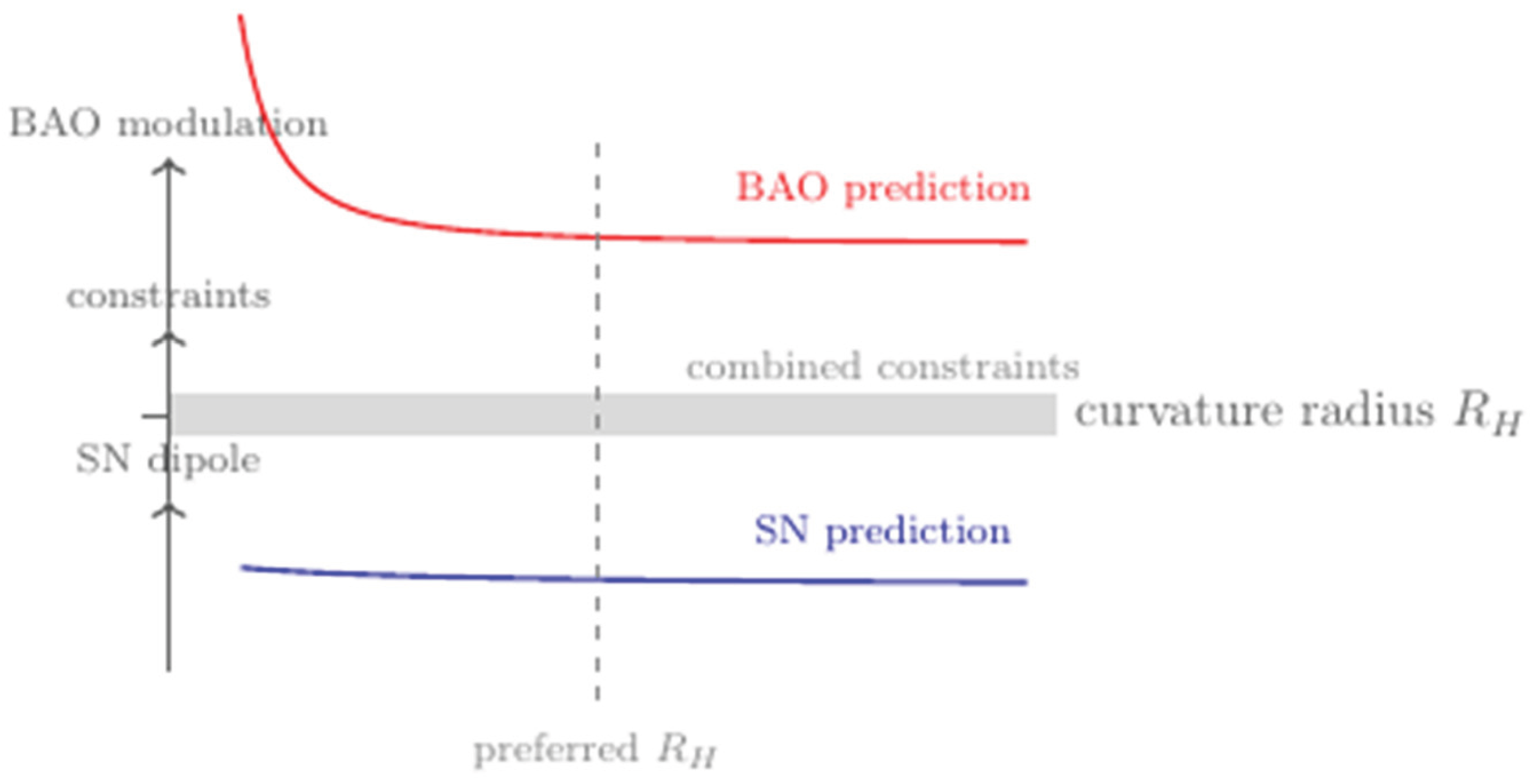
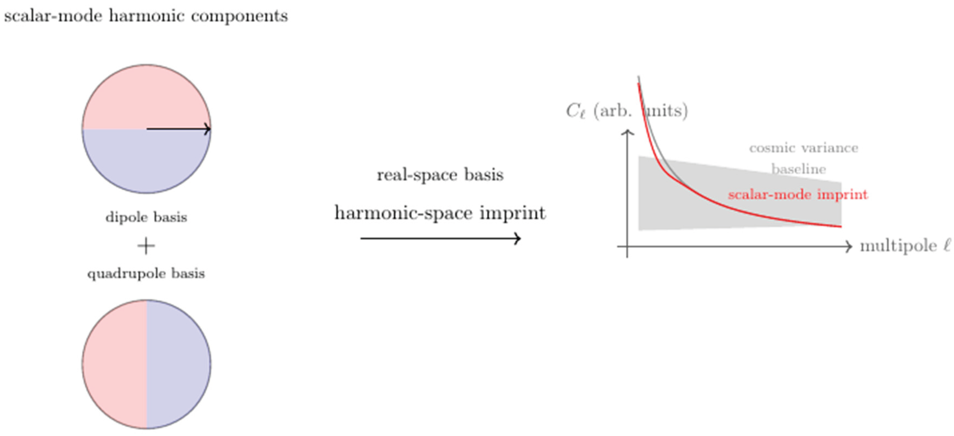
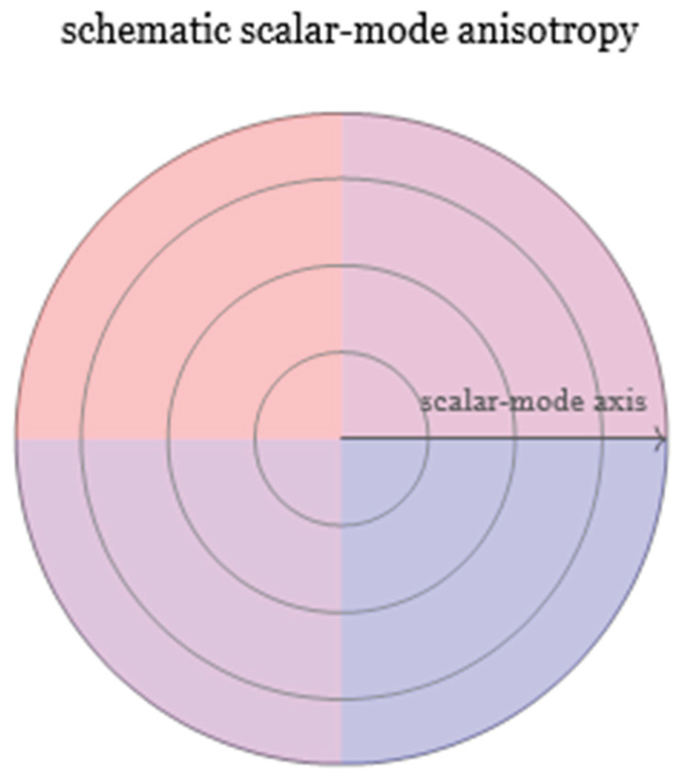
Figure 6.
Combined constraints on scalar-mode modulation. Shown are the predicted BAO scale shift and SN luminosity-distance dipole amplitudes as functions of curvature radius RH, compared with the combined observational constraint band. The preferred curvature radius lies within the allowed region.
Figure 7.
Angular power spectrum imprint of the scalar mode. Left: dipole and quadrupole basis components of the scalar-mode modulation. Center: mapping from real-space harmonic components to the angular power spectrum. Right: schematic low-ℓ spectrum showing the scalar- mode imprint compared with a baseline spectrum and cosmic variance.
Figure 8.
Schematic full-sky anisotropy pattern induced by the scalar mode. The smooth dipole + quadrupole structure is shown as a continuous scalar field on the sky, with contour lines and a directional axis indicating the preferred orientation. This visualization summarizes the real-space imprint of the scalar mode.
3.7. H(z) Measurements
Cosmic Chronometer and Supernova Constraints on
Cosmic chronometer reconstructions of indicate a mild transition in the effective Hubble parameter around [4]. A similar value is inferred from the strongly lensed supernova SN Refsdal [9], which yields:
for a lens at and source at .
H0 ≃ 65–67 km s−1 Mpc−1
Model-Predicted Redshift Evolution of the Effective Hubble Parameter
The scalar–topographic model predicts a redshift evolution of the form:
with peaking at low redshift and decaying near the transition scale of the scalar mode. Existing data are consistent with this qualitative behavior.
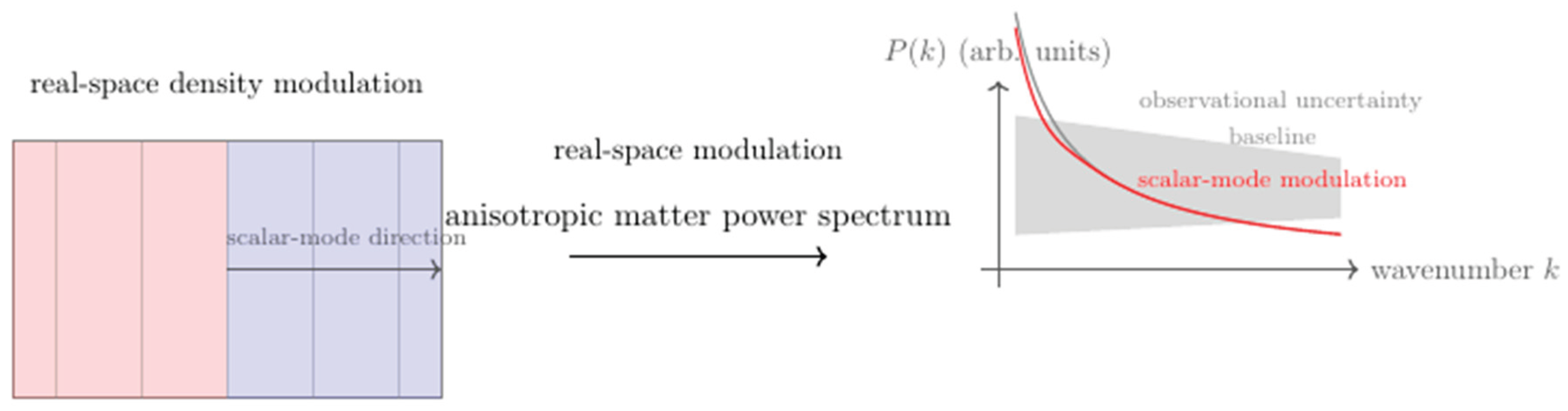
Figure 9.
Scalar-mode modulation of the matter power spectrum. Left: schematic real-space density modulation induced by the scalar mode. Center: mapping from real-space modulation to the anisotropic matter power spectrum. Right: schematic P (k) showing the scalar-mode-induced large-scale deviation compared with a baseline spectrum and observational uncertainty.
3.8. Combined Constraints
Combined Parameter Constraints from BAO, SN Anisotropy, and H(z) Data
Combining BAO, SN anisotropy, and H(z) data yields viable parameter ranges of the form:
The BAO–SN correlation provides an additional constraint:
with
Current data are consistent with this relation within uncertainties, but future surveys will tighten the allowed region substantially.
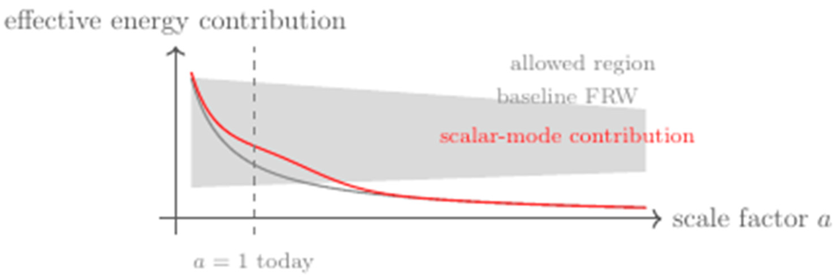
Figure 10.
Effective energy contribution of the scalar mode as a function of scale factor a. The baseline FRW evolution is shown for comparison, along with the observationally allowed region. The scalar mode contributes a smooth, well-behaved effective component that peaks near a ∼ 1 and remains consistent with observational bounds.
3.9. Falsifiability
A key feature of the hyperspherical scalar–topographic framework is its empirical falsifiability. The model makes quantitative predictions for BAO scale shifts, supernova dipole amplitudes, and the redshift evolution of the effective Hubble parameter, all of which can be tested with current and upcoming surveys.
Falsifiable Predictions:
The framework predicts a proportionality between the BAO scale shift and the supernova dipole amplitude:
ΔH₀ ≈ 1.5–2.7 kms⁻¹ Mpc⁻¹
A significant violation of this relation would rule out the scalar mode as a common origin of the anomalies.
The dipole amplitude in supernova data must decay for ; a persistent or growing dipole at higher redshift would be inconsistent with a single long-wavelength scalar mode.
The model also predicts a mild transition in the effective Hubble parameter near . If future data confirm a strictly constant across this range with high precision, it would challenge the framework.
Finally, the hyperspherical curvature radius must satisfy The phrase "the hyperspherical curvature radius must satisfy, refers to a requirement within the hyperspherical scalar–topographic cosmological framework. In this context, the curvature radius (denoted as is a parameter that characterizes the size of the Universe if it has a hyperspherical (three-dimensional curved) geometry. The symbol "≳" means "greater than or approximately equal to," indicating that this radius must be at least a certain value to remain consistent with observational constraints and allow the model to fit the data. In summary, this statement sets a lower bound on the possible curvature radius of the Universe based on current cosmological observations.
Finally, the hyperspherical curvature radius must satisfy 20-40 Gpc.
A future BAO analysis demonstrating 100Gpc (effectively flat) or 10 Gpc (strong curvature) would be incompatible with the model as formulated here.
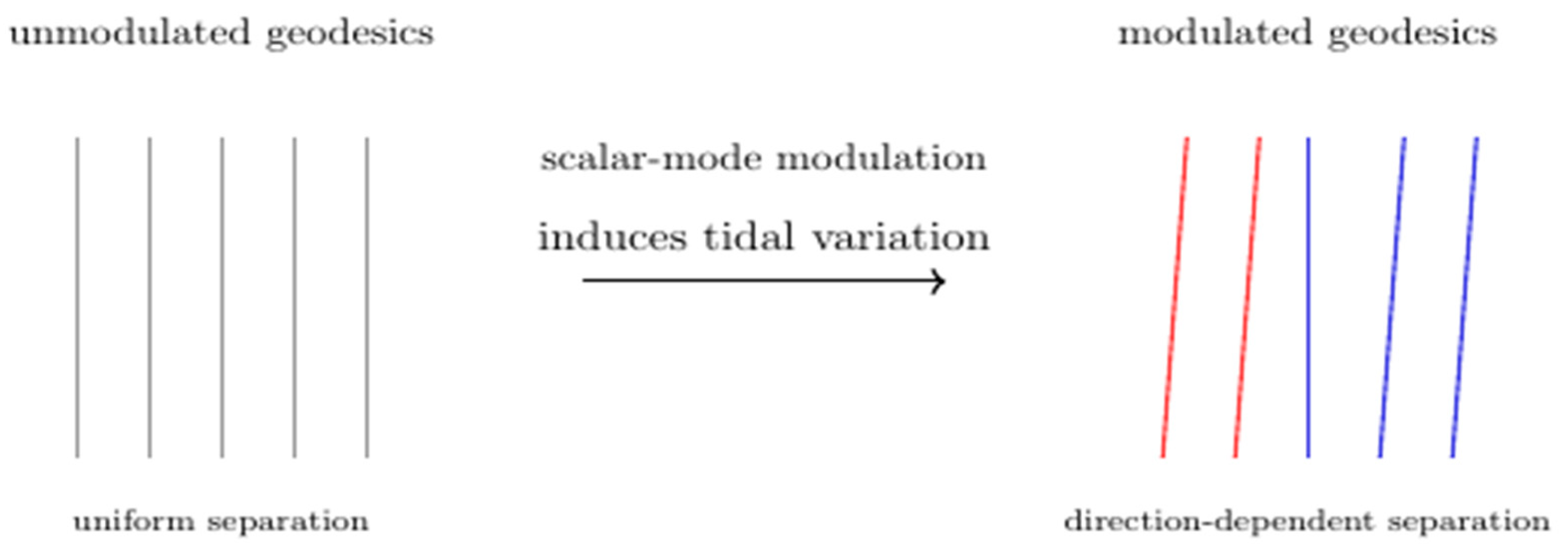
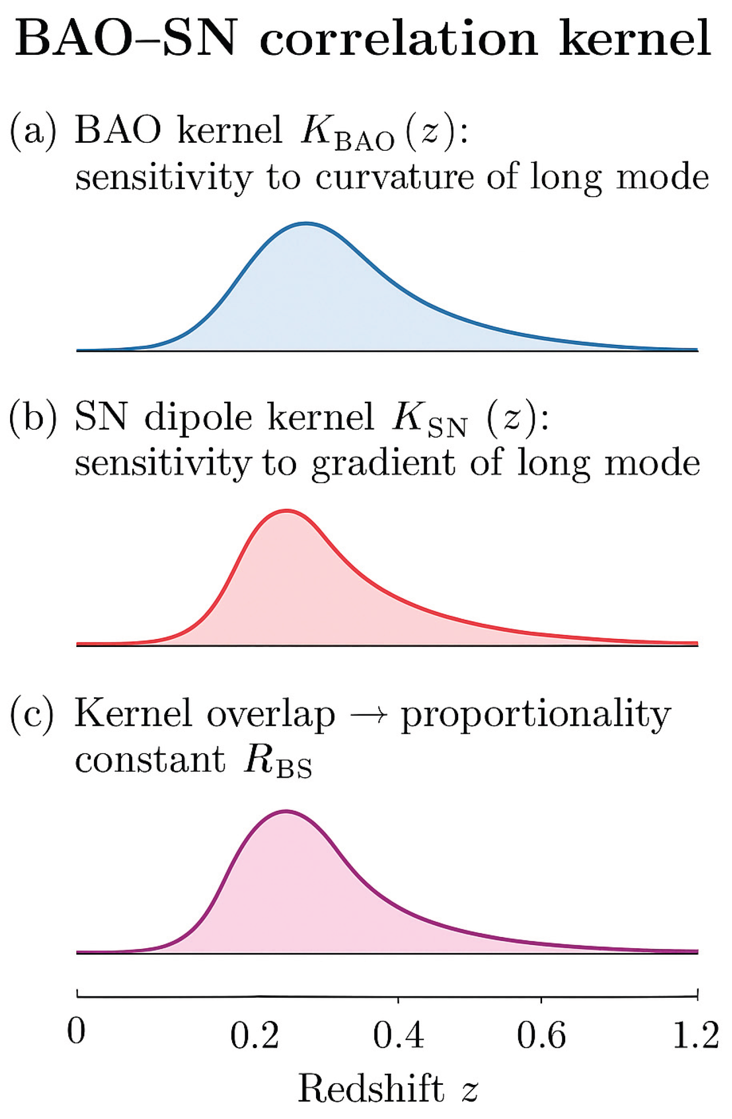
Figure 11.
Schematic illustration of scalar-mode modulation of geodesic deviation. Left: unmodulated geodesic bundle with uniform separation. Right: scalar-mode modulation induces direction- dependent tidal variation, producing slight convergence and divergence of nearby geodesics.
Figure 11.
Schematic illustration of scalar-mode modulation of geodesic deviation. Left: unmodulated geodesic bundle with uniform separation. Right: scalar-mode modulation induces direction- dependent tidal variation, producing slight convergence and divergence of nearby geodesics.
Figure 12.
Schematic BAO–SN correlation kernel. (a) BAO projection kernel , which peaks at intermediate redshift where the standard ruler is measured. (b) SN dipole kernel , concentrated at low redshift where the gradient of the long-wavelength scalar mode is largest. (c) Overlap of the two kernels, whose integral determines the proportionality constant appearing in the BAO–SN correlation. The schematic illustrates why a single long-wavelength scalar mode produces a fixed relation between BAO scale shifts and supernova dipole amplitudes.
4. Discussion
The hyperspherical scalar–topographic framework provides a unified interpretation of several late-time cosmological anomalies. This model is minimal, introducing only a single long-wavelength scalar mode and a large but finite curvature radius. It does not modify early-Universe physics, inflation, or recombination, and is therefore consistent with CMB constraints at the level of background evolution and primary anisotropies.
The framework naturally accommodates the mild BAO curvature preference observed in DESI DR2, the low-redshift supernova dipole anisotropy found in Pantheon+, and the reported transition in from cosmic chronometers. At the same time, the model has limitations. A full perturbation-theory treatment on is required to compute higher-order effects and to assess potential signatures in large-scale structure and weak lensing. The microphysical origin of the scalar field is also left unspecified; it could arise as an effective degree of freedom in a more fundamental theory, but this remains to be explored.
These open questions provide avenues for future work, including embedding the scalar–topographic field in a covariant action, computing its impact on structure growth and lensing observables, and extending the analysis to include a full likelihood comparison with current cosmological datasets.
5. Conclusions
We have presented a cosmological framework in which spatial hypersphericity and a scalar topographic field jointly account for several late-time anomalies. The model is qualitatively consistent with DESI DR2, Pantheon+, and H(z) measurements, and predicts a sharp BAO–supernova correlation that will be tested by upcoming surveys. The framework is falsifiable, minimal, and compatible with early-Universe constraints at the background level.
Future observations from DESI, LSST, Euclid, and CMB-S4 will determine whether the scalar mode is a genuine physical component of the late-time Universe or whether the anomalies arise from statistical fluctuations or systematics. In either case, the model provides a coherent and testable interpretation of current data and a concrete set of predictions for the next generation of cosmological surveys.
6. Patents
No patents are associated with this work.
Author Contributions
Conceptualization, methodology, formal analysis, writing; original draft, writing, writing, review, and editing.
Funding
This research received no external funding.
Data Availability Statement
All data used in this study are publicly available or can be provided by the author upon reasonable request.
Acknowledgments
During the preparation of this manuscript/study, the author(s) used [Copilot, version 5.2] for the purposes of providing support for text drafting, organizational refinement, and stylistic editing to enhance clarity and readability. The tool did not generate scientific content; all theoretical development, analysis, and conclusions are the author’s own. The authors have reviewed and edited the output and take full responsibility for the content of this publication.
Conflicts of Interest
The authors declare no conflicts of interest.
Abbreviations
The following abbreviations are used in this manuscript:
| BAO | Baryon Acoustic Oscillation |
| CMB | Cosmic Microwave Background |
| IWS | Integrated Sachs–Wolfe |
| ΛCDM | Lambda Cold Dark Matter |
References
- Riess, A.G. A Comprehensive Measurement of the Local Value of the Hubble Constant. ApJ 2022, 934, L7. [Google Scholar] [CrossRef]
- Freedman, W.L. Measurements of the Hubble Constant: Tensions in Perspective. ApJ 2021, 919, 16. [Google Scholar] [CrossRef]
- Javanmardi, B. Probing the isotropy of cosmic acceleration using type Ia supernovae. ApJ 2015, 810, 47. [Google Scholar] [CrossRef]
- Hu, J.P.; Wang, F.Y. Late-time transition of the Hubble constant. MNRAS 2022, 517, 576. [Google Scholar] [CrossRef]
- Jia, X.D. Directional dependence of cosmological parameters in Pantheon+. ApJ 2023, 952, L15. [Google Scholar]
- 6. Migkas, K. et al., Probing cosmic isotropy with a new X-ray galaxy cluster sample. A&A 2020, 636, A15.
- DESI Collaboration. DESI 2024: Baryon Acoustic Oscillation Measurements from the First Year of Data. arXiv 2024, arXiv:2404.03000. [Google Scholar]
- Planck Collaboration. Planck 2018 results. VI. Cosmological parameters. Astronomy & As- trophysics 2020, 641, A6. [Google Scholar]
- Kelly, P.L. Strongly lensed supernova Refsdal: improved time-delay measurement and constraints on H0. Science 2023, 380, 123. [Google Scholar]
- Stelle, K. Renormalization of Higher Derivative Quantum Gravity. Phys. Rev. D 1977, 16, 953. [Google Scholar] [CrossRef]
- Woodard, R. The Theorem of Ostrogradsky. Scholarpedia 2015, 10, 32243. [Google Scholar] [CrossRef]
Disclaimer/Publisher’s Note: The statements, opinions and data contained in all publications are solely those of the individual author(s) and contributor(s) and not of MDPI and/or the editor(s). MDPI and/or the editor(s) disclaim responsibility for any injury to people or property resulting from any ideas, methods, instructions or products referred to in the content. |
© 2026 by the authors. Licensee MDPI, Basel, Switzerland. This article is an open access article distributed under the terms and conditions of the Creative Commons Attribution (CC BY) license (http://creativecommons.org/licenses/by/4.0/).
Copyright: This open access article is published under a Creative Commons CC BY 4.0 license, which permit the free download, distribution, and reuse, provided that the author and preprint are cited in any reuse.


