
Submitted:
17 January 2026
Posted:
19 January 2026
You are already at the latest version
Abstract
Background/Objectives: Patients with breast cancer show substantial heterogeneity in psychological adjustment following diagnosis. We aim to characterize longitudinal trajectories of quality of life (QoL) and depressive symptoms during the first 18 months post-diagnosis and to identify robust clinical, psychosocial, and behavioral predictors associated with distinct adjustment pathways. Methods: Data were drawn from the multicenter BOUNCE cohort. QoL (EORTC QLQ-C30) and depressive symptoms (HADS) were assessed repeatedly over 18 months. Latent Class Growth Analysis and Growth Mixture Modeling were used to identify distinct trajectory classes. Associations between candidate predictors and trajectory membership were ex-amined using logistic regression combined with elastic net regularization, including clinically motivated binary contrasts. Predictor robustness was evaluated under models with clinical site alternatively penalized and unpenalized. Results: Depression trajectories demonstrated heterogeneity, with groups characterized by persistent resilience (59.7%), stable moderate/high depression (25.3%), delayed-onset de-pression (5.0%), and recovery (10.0%). QoL trajectories ranged from stable excellent (13.2%) and stable high (13.2%) functioning to persistent low or deteriorating QoL (6.9%), with a distinct recovery trajectory (7.8%). Trajectory differentiation was primarily driven by psychological resources, symptom burden, functional status, and coping processes, while selected clinical factors contributed to specific trajectories. Patterns of predictors dif-fered across trajectory contrasts. Conclusions: Distinct subgroups of women with breast cancer follow divergent QoL and depres-sion trajectories after diagnosis. Differences between trajectories are shaped by a combination of psychological, functional, and clinical factors, highlighting the multidimensional nature of resilience and recovery. These findings support the need for tailored interven-tions that move beyond risk reduction toward promoting long-term well-being and mental health.
Keywords:
in silico medicine
; in silico psycho-oncology
; machine learning
; artificial intelligence
; breast cancer
; resilience
; depression
; quality of life
1. Introduction
Patient resilience is a critical determinant of cancer treatment outcomes, influencing both psychological adaptation and overall quality of life [1]. Higher levels of resilience have been associated with younger age, female sex, higher socioeconomic status and being married, as well as with internal psychological resources such as optimism, self-efficacy and adaptive emotion regulation strategies and external resources such as social support [2,3,4]. Positive cognitive strategies, including acceptance and positive thinking, are linked to enhanced psychological well-being, whereas maladaptive strategies such as rumination and catastrophizing are consistently associated with adverse emotional outcomes [5,6,7,8,9,10,11]. Among women with breast cancer, optimism and self-efficacy predict better psychological well-being, improved quality of life and lower distress over time [12,13], while perceived social and family support facilitates adaptive coping and resilience [14,15,16,17].
Within this context, the EU-funded BOUNCE project (https://www.bounce-project.eu/; accessed 20 December 2025) conducted a prospective multicenter clinical study across Finland, Italy, Portugal and Israel to investigate predictors of resilience trajectories among women with breast cancer. The study collected a thorough range of sociodemographic, clinical, psychological and functional factors with the aim of improving the ability to predict resilience in response to breast cancer and, ultimately, to inform personalized interventions that promote effective psychological recovery.
The aim of the current study is twofold: (1) to identify distinct longitudinal trajectories of depression and quality of life (QoL) over the 18 months following diagnosis and/or surgery and (2) to identify factors associated with these trajectories, with particular focus on patterns reflecting resilience, recovery, deterioration and persistent impairment. To address the first aim, we apply latent class growth analysis (LCGA) and growth mixture modelling (GMM), methods widely used in psycho-oncology to capture heterogeneity in longitudinal symptom and QoL patterns. To address the second aim, we use logistic regression models to examine associations between candidate predictors and trajectory membership, allowing results to remain clinically interpretable. In addition to univariate analyses, we perform multivariable feature selection using elastic net regularization. Feature selection is used to identify parsimonious sets of predictors that jointly differentiate trajectory groups, while accounting for correlations between variables and limiting overfitting. This approach moves beyond isolated univariate associations and supports clearer interpretation of factors relevant for personalized risk assessment and intervention.
To capture clinically meaningful heterogeneity in longitudinal mental health and quality-of-life (QoL) outcomes, we focus on selected comparisons between trajectory groups that address complementary research questions. Specifically, we examine:
- Who remains resilient over time, compared with individuals who experience persistently elevated depressive symptoms or persistently lower QoL, thereby capturing differences in long-term outcome levels.
- Who is at risk for persistently poor depression or QoL outcomes, providing insight into profiles associated with sustained vulnerability.
- Who deteriorates despite early resilience, a contrast that is less confounded by baseline outcome levels and enables the identification of early warning markers relevant to preventive strategies, clinical monitoring and early intervention.
- Who recovers among individuals with comparable baseline levels, a comparison that is likewise less influenced by baseline outcome levels and highlights factors associated with improvement rather than symptom burden, with potential implications for therapeutic intervention.
2. Materials and Methods
2.1. Participants
The BOUNCE project (“Predicting Effective Adaptation to Breast Cancer to Help Women to BOUNCE Back”) is a multicenter prospective study designed to identify factors associated with psychological adaptation following breast cancer diagnosis and treatment (https://www.bounce-project.eu/; accessed 20 December 2025). Women diagnosed with breast cancer were recruited from four European countries: Finland (Helsinki University Hospital), Israel (Shaare Zedek Medical Center and Rabin Medical Center, coordinated by the Hebrew University of Jerusalem), Italy (European Institute of Oncology) and Portugal (Champalimaud Clinical Centre). Participants were enrolled approximately three to four weeks from diagnosis.
Eligible participants were female patients aged 40–70 years at diagnosis with histologically confirmed, operable invasive breast cancer (tumor stage I–III), who were receiving surgery as part of local treatment and any form of systemic therapy for breast cancer and who provided written informed consent signed by both the patient and the treating physician. Exclusion criteria included refusal to consent; presence of metastatic disease or a history of another malignancy within the previous five years; a history of severe psychiatric, neurological, (before 40 years of age) or other serious medical conditions; major surgery within the four weeks preceding enrollment; ongoing treatment for another invasive cancer or major illness; and pregnancy or breastfeeding at the time of recruitment. Ethical approval was obtained from the Ethics Committee of the European Institute of Oncology (Approval No. R868/18-IEO916) and from the corresponding ethics committees of all participating centers, while all participants provided written informed consent prior to inclusion.
Data were collected at seven assessment points at three-month intervals, from baseline (M0) to 18 months of follow-up (M18). Psychological symptoms and subjective health status were assessed at all time points, whereas sociodemographic, lifestyle and medical or disease-related variables considered in this analysis were collected at baseline [study protocol at [18]. After applying eligibility criteria and data completeness requirements, the final analytic sample consisted of 538 patients with baseline psychological assessments, at least one long-term follow-up assessment (month 12, 15, or 18) and no more than three missing assessments across the 18-month follow-up period.
2.2. Measures
2.2.1. Outcome Variables
Two outcome variables are considered reflecting psychological distress and health-related quality of life.
Psychological distress was measured using the Depression subscale of the Hospital Anxiety and Depression Scale [19] (HADS). It derives from seven items of the HADS questionnaire, with higher scores (range 0-3 – mean scale) indicating greater severity of depressive symptoms. HADS Depression score was interpreted using established thresholds, with scores of 0–1 indicating low depressive symptoms (corresponding to 0–7 on the 0–21 scale), 1.14–1.42 moderate symptoms (8-10 on the 0-21 scale) and ≥1.57 high symptomatology (≥11 on the 0-21 scale) [20]. Longitudinal changes were interpreted based on published minimally important difference criteria, whereby changes of approximately 0.2–0.43 points were considered clinically meaningful and changes of ≥0.43 points indicative of moderate to large clinical change [21,22,23].
Overall health-related quality of life was assessed using the Global Health Status/Quality of Life [24] (GHS/QoL) scale of the European Organisation for Research and Treatment of Cancer Quality of Life Questionnaire C30 (EORTC QLQ-C30). This scale reflects patients’ self-reported overall health and quality of life and is derived from two items of the EORTC QLQ-C30, with higher scores (range 0–100) indicating better well-being. As no official clinical cut-offs are defined, interpretation of absolute GHS/QoL levels was guided by published empirical thresholds, with scores ≥70 considered indicative of good to excellent quality of life, scores between approximately 50 and 69 reflecting moderate quality of life and scores <50 indicating poor quality of life [25,26]. Longitudinal changes in GHS/QoL were interpreted using established minimally important difference criteria, with changes of 5–10 points considered small but clinically meaningful and changes ≥10 points considered moderate to large [27].
2.2.2. Sociodemographic, Lifestyle and Clinical Data
The analysis incorporated socioeconomic and lifestyle factors, health-related background variables and tumor and treatment characteristics collected at baseline (Table 1).
Socioeconomic and lifestyle data collected at baseline included age, body mass index (BMI), ethnicity (Portugal; Italy; Finland; Israel), educational attainment (non-University; University), marital status (single/engaged; married/common-law; divorced/widowed), employment status (employed full-/part-time or self-employed; unemployed/housewife; retired) and monthly household income (low; middle; high). Low monthly income was defined as ≤1,000 EUR in moderate-income countries (Portugal, Italy) and ≤1,500 EUR in higher-income countries (Finland, Israel), whereas high income was defined as >3,000 EUR and >3,500 EUR, respectively.
Lifestyle factors included physical activity level (none; low/moderate; heavy), dietary pattern (no specific diet; Mediterranean/vegetarian-type; special diet), alcohol consumption (no consumption; moderate consumption; heavy consumption) and smoking status (current smoker; never smoker; former smoker). Heavy alcohol consumption was defined as intake of more than three drinks on any day or more than seven drinks per week. Heavy physical activity was defined as ≥200 minutes per week of moderate aerobic activity or ≥100 minutes per week of vigorous aerobic activity; or ≥5 weekly strength-training sessions; or combined aerobic and strength activity meeting ≥100–180 minutes per week of moderate (or ≥50–90 minutes per week of vigorous) aerobic exercise with ≥1–4 weekly strength sessions.
Health history variables included presence of chronic diseases (no/yes), metabolic diseases (no/yes), mental illness (no/yes), exposure to negative life events (none; one event; two or more events) and family history of breast cancer (no/yes). These variables were considered background health factors potentially, treatment tolerance and psychological outcomes.
Clinical and cancer-related data included menopausal status prior to cancer diagnosis (pre-/peri-menopausal; postmenopausal), use of hormone replacement therapy before diagnosis (no/yes), tumor stage (I, II, III), tumor grade (I, II, III) and histological subtype (ductal; lobular; other). Tumor biomarker characteristics comprised estrogen receptor (ER) status (negative/positive), progesterone receptor (PR) status (negative/positive), human epidermal growth factor receptor 2 (HER2) status (negative/positive) and Ki67 proliferation index (<20%; ≥20%). Molecular subtypes were defined as Luminal A-like (ER+, PR+, HER2−, low Ki67 <20%); Luminal B-like (HER2−: ER+, PR+/− with high Ki67 ≥20% or ER+, PR− with any Ki67; or HER2+: ER+, PR+/− with any Ki67); HER2-positive non-luminal (ER−, PR−, HER2+); and triple-negative (ER−, PR−, HER2−). Treatment-related variables included type of surgery (lumpectomy; mastectomy), receipt of radiotherapy (no/yes), systemic treatment modality (chemotherapy only [± anti-HER2 therapy], endocrine therapy only, or combined chemotherapy and endocrine therapy [± anti-HER2 therapy]), use of anti-HER2 therapy (no/yes) and administration of neoadjuvant chemotherapy (no/yes).
2.2.3. Psychological Scales
Psychological variables were assessed using validated self-report questionnaires administered at predefined time points throughout follow-up. Relatively stable personality and psychosocial characteristics were assessed at baseline, including optimism using the Life Orientation Test–Revised [28] (LOT-R; 10 items), sense of coherence using the Sense of Coherence Scale [29] (SOC; 13 items assessing meaningfulness, comprehensibility and manageability), trait resilience using the Connor–Davidson Resilience Scale [30] (CD-RISC; 10 items), dispositional mindfulness using the Mindful Attention Awareness Scale [31] (MAAS; 15 items) and general coping capacity using the Perceived Ability to Cope with Trauma Scale [32] (PACT; 20 items). Cancer coping self-efficacy was measured using the brief Cancer Behavior Inventory [33] (CBI-B; 12 items) and Fear of cancer recurrence was also assessed using the Fear of Cancer Recurrence Scale–Short Form [34] (FCR-SF; 9 items), both at baseline. Coping responses to cancer were assessed at three months post-diagnosis using the Mini–Mental Adjustment to Cancer Scale [35] (Mini-MAC; 29 items assessing helplessness–hopelessness, anxious preoccupation, cognitive avoidance and fighting spirit; the fatalism dimension was excluded from analyses). Post-traumatic growth was measured at three months using the Post-Traumatic Growth Inventory–Short Form [36] (PTGI-SF; 10 items).
Anxiety symptoms were assessed every three months using the the Hospital Anxiety and Depression Scale [19] (HADS; 7 items). Emotional functioning was assessed longitudinally every three months using the Positive and Negative Affect Schedule [37] (PANAS; 20 items), while health-related quality of life, including patients’ functioning status and symptom burden (e.g., arm symptoms and treatment-related side effects), was assessed every three months using the European Organisation for Research and Treatment of Cancer Quality of Life Questionnaire-Core 30 [24] (EORTC QLQ-C30) and its breast cancer–specific module [24] (EORTC QLQ-BR23).
Several single-item measures were additionally collected to capture specific psychosocial and behavioral aspects. These included a single item assessing what patients reported doing to cope with cancer, a general self-efficacy item and a perceived social support item, all assessed every three months. Adherence to medical advice was assessed using item 5 from the Medical Outcomes Study [38] (MOS) adherence questionnaire.
2.3. Statistical Analysis
2.3.1. Missing Data
Missing data were addressed using multiple imputation by chained equations (mice R package [39]), generating 30 or 50 imputed datasets, depending on the proportion of missingness. All candidate predictors, outcomes and the clinical site variable were included in the imputation models to preserve associations among variables. The random forest–based method was selected.
2.3.2. Derivation of Mental Health and GHS/QoL Trajectories
Latent class growth analysis (LCGA) and growth mixture modelling (GMM) were conducted using the lcmm package in R [40] to identify discrete longitudinal trajectories among breast cancer survivors based on EORTC QLQ-C30 GHS/QoL and HADS Depression scores over an 18-month follow-up period. Separate analyses were performed for each outcome. LCGA is a restricted form of GMM in which within-class variances of the random intercept and slope are fixed to zero, allowing heterogeneity only between classes. As random effects are not permitted within classes, LCGA typically requires a larger number of latent classes to adequately capture variability in the data compared with GMM.
To account for non-normal outcome distributions, a six-knot I-spline link function was applied. The choice of link function was informed by preliminary analyses of the null (single-class) model (Appendix A).
Quadratic models of the change across time were considered. For GMM, models with one to six latent classes were estimated, while for LCGA models with one to eight latent classes were considered. Each model was estimated multiple times using a grid of 250 sets of initial values to reduce the risk of convergence to local maxima. For each specified number of latent classes, the model with the highest log-likelihood was retained.
Model selection and determination of the optimal number of latent classes were based on a combination of statistical fit indices, class separation, trajectory shapes, minimum class size, interpretability and clinical relevance [41]. Fit was assessed using the Akaike Information Criterion (AIC), Bayesian Information Criterion (BIC) and Integrated Complete Likelihood (ICL), with lower values indicating better fit [41]. Both AIC and BIC balance model fit and complexity, but BIC imposes a stronger, sample-size–dependent penalty and therefore typically selects more parsimonious solutions with fewer latent classes. The ICL further penalizes solutions with poor class separation, jointly accounting for model fit and classification quality. Class separation was further evaluated using entropy and average posterior class membership probabilities, with values greater than 0.60 and 0.70, respectively, indicating adequate separation [42,43]. A minimum class size of at least 5% of the total sample was required.
The lcmm framework accommodates missing outcome data, therefore, no imputation of outcome variables was performed.
2.3.3. Determinants of Mental Health and GHS/QoL Trajectories
Once the trajectory groups were identified, binomial logistic regression was conducted to determine which factors at baseline, three-month and six-month follow-up are associated with trajectory group membership.
Initially, associations between individual predictors and the outcome were examined using logistic regression models adjusted for clinical site across imputations. Clinical site was included as a fixed-effect adjustment variable to account for between-site heterogeneity and results were pooled using Rubin’s rules to obtain odds ratios and 95% confidence intervals that reflect uncertainty due to missing data.
Variable selection was conducted using penalized logistic regression with an elastic net penalty, implemented in R using the glmnet package [44] (glmnet and cv.glmnet functions). The elastic net approach was chosen to balance variable selection and coefficient shrinkage while accommodating correlated predictors, which are common in clinical, quality-of-life, and psychosocial data. This strategy supported the identification of robust predictors while maintaining model interpretability and reducing the risk of overfitting. The elastic net mixing parameter was set to α = 0.5, providing an equal balance between L1 (LASSO) and L2 (ridge) penalties to achieve stable variable selection in the presence of correlated predictors [45]. Candidate predictors were encoded using model matrices (model.matrix), such that categorical variables were represented by indicator variables. The regularization parameter (λ) was selected via 10-fold cross-validation with stratified folds to preserve outcome class proportions within each fold and mitigate the impact of class imbalance. To promote stable and parsimonious models and reduce the risk of overfitting, the one-standard-error rule (λ₁se) was used for λ selection [46]. Cross-validation was performed using deviance as the optimization criterion, corresponding to the negative log-likelihood of the logistic model, thereby favoring predictors that improve probabilistic calibration rather than threshold-dependent classification accuracy. The selection procedure was repeated 3 times across all multiple imputed datasets generated using the mice package (see 3.3.1) and predictor importance was quantified by selection frequency across imputations and 3 repeats. To evaluate the robustness of our predictors, we conducted the stability analysis under two conditions. Clinical sites were treated as standard predictors subject to the L1/L2 penalty and clinical sites were forced into the model by setting their penalty factor to zero, ensuring their inclusion in every iteration regardless of the regularization threshold. This allowed us to distinguish site-independent predictors from variables reflecting differences in healthcare systems, socioeconomic contexts, and cultural factors. Predictors with high selection frequency (>60%) under both penalized and unpenalized site conditions were considered robust. Descriptive penalized odds ratios were reported to indicate the direction and relative magnitude of associations at the selected regularization parameter under the initial penalized site condition.
Model performance was evaluated using cross-validated predictions from elastic net logistic regression models, with metrics computed on held-out data and averaged across folds, thus reflecting out-of-sample performance. Performance was assessed using ROC-AUC, log-loss, and the Brier score, capturing complementary aspects of predictive quality. ROC-AUC quantifies discrimination, whereas log-loss and the Brier score assess probabilistic accuracy and calibration, with lower values indicating better performance. Although no strict cut-offs exist, ROC-AUC values of 0.60-0.70 indicate poor-to-fair discrimination, 0.70-0.80 acceptable, 0.80-0.90 very good, and >0.90 excellent discrimination [47]; Brier score and log loss were interpreted against chance-level (null-model) values, corresponding to predictions equal to the observed outcome prevalence.
Clinical site was included among candidate predictors during the elastic net selection procedure to assess its stability and potential predictive contribution.
3. Results
3.1. Baseline Demographic and Clinical Characteristics
The study cohort comprised women with a mean age of 55.4 years (40-70) recruited across four countries, most commonly Finland (38.1%), followed by Portugal (24.9%), Israel (19.3%) and Italy (17.7%). The majority had a University education (60.7%), were married or living with a partner (74.9%) and were employed (72.9%), with most reporting middle income levels (61.6%). Regarding lifestyle characteristics, two thirds reported engaging in exercise (66.3%), almost half followed a type of diet (45.4%), most consumed alcohol in moderation (68.2%) and the majority were never smokers (67.4%).
Clinically, most participants were postmenopausal (61.5%), had stage I–II disease (91.0%), grade II tumors (52.2%) and ductal histology (77.9%). Tumors were predominantly hormone receptor–positive (ER-positive 89.6%; PR-positive 79.8%) and HER2-negative (81.8%), with luminal A-like (36.9%) and luminal B-like HER2-negative (39.0%) subtypes being most frequent. Breast-conserving surgery was the most common surgical approach (74.6%), radiotherapy was administered to 80.6% of patients and systemic treatment most often consisted of endocrine therapy alone (47.3%) or combined chemotherapy and endocrine therapy (37.7%).

Table 2.
Baseline clinical and cancer characteristics of the study participants. Total number of patients n=538.
Table 2.
Baseline clinical and cancer characteristics of the study participants. Total number of patients n=538.
| Variable | n (%) | Variable | n (%) |
|---|---|---|---|
| Negative Life Events | Estrogen receptor Positivity | 467 (89.6%) | |
| None | 58 (12%) | Progesterone receptor Positivity | 410 (79.8%) |
| One event | 239 (49.6%) | HER2 Positivity | 89 (18.2%) |
| Two or more events | 185 (38.4%) | Ki67 levels ≥20% | 293 (56.7%) |
| Chronic diseases | 191 (35.7%) | Subtypes1 | |
| Metabolic diseases | Luminal A-like | 175 (36.9%) | |
| Mental illness | Luminal B-like (HER2 -) | 185 (39%) | |
| Family history of beast cancer | 330 (64.3%) | Luminal B-like (HER2 +) | 68 (14.3%) |
| Menopausal status pre | Her2-positive (non luminal) | 20 (4.2%) | |
| Pre/Peri-menopausal | 202 (38.5%) | Triple-negative | 26 (5.5%) |
| Postmenopausal | 322 (61.5%) | Lumpectomy | 391 (74.6%) |
| HRT before diagnosis | 105 (21.6%) | Mastectomy | 133 (25.4%) |
| Cancer stage | Radiotherapy | 424 (80.6%) | |
| I | 251 (48.2%) | Systemic Therapy | |
| II | 223 (42.8%) | Chemotherapy only (± anti-HER2) | 78 (14.9%) |
| III | 47 (9%) | Endocrine therapy only | 247 (47.3%) |
| Cancer grade | Chemo + Endocrine therapy (± anti-HER2) | 197 (37.7%) | |
| I | 91 (17.5%) | Anti-HER2 therapy | 82 (15.4%) |
| II | 271 (52.2%) | Neoadjuvant Chemotherapy | 84 (16%) |
| III | 157 (30.3%) | ||
| Cancer histological type | |||
| Ductal | 408 (77.9%) | ||
| Lobular | 80 (15.3%) | ||
| Other | 36 (6.9%) |
1Luminal A-like: ER+, PR+, HER2-, low Ki67 (<20%); Luminal B-like (HER2 negative): ER+, PR+/-, HER2-, high Ki67 (≥20%) or ER+, PR-, HER2-, Ki67 any; Luminal B-like (HER2 positive): ER+, PR+/-, HER2+, any Ki67; Her2-positive (non luminal) ER-, PR-, HER2+, any Ki67; Triple-negative (ER-, PR-, HER2-, any Ki67) Abbreviations: HRT: Hormone Replacement Therapy; HER2: human epidermal growth factor receptor 2.
3.2. Trajectory Groups
3.2.1. GHS/QoL Trajectories
Taking into account statistical fit, class separation, parsimony and clinical interpretability, we selected the five-class LCGA solution as the optimal model (See Appendix B for detailed explanations). Figure 1a shows the resulting trajectories for the five-group model and the actual measurements of the patients that compose each class. An Excellent trajectory (n = 71, 13.2%) demonstrated very high baseline scores (≥90) that remained stable throughout the study period. Mean increase in slope is statistically significant (Table D1 in Appendix D) but overall changes are small (<5–10 points), indicating no clinically meaningful change over time, while individual trajectories cluster tightly at high values with limited variability. The largest class was the Good trajectory (n = 219, 40.7%), characterized by consistently high QoL scores primarily within the good range (≥70). The mean trajectory was essentially flat (Table D1 in Appendix D). This class exhibited greater individual variability than the Excellent class; however, most observations remained ≥70 throughout follow-up. The Moderate class (n = 169, 31.4%) exhibited baseline and follow-up scores predominantly within the moderate range (50–69). Substantial within-class variability was observed, with some individuals showing improvement over time while others remained stable or fluctuated across follow-up. Overall, the mean trajectory remained largely stable (Table D1 in Appendix D). A small Recovering class (n = 42, 7.8%) started with moderately reduced QoL (approximately 60–65) but exhibited a marked and sustained improvement exceeding clinically important change thresholds (≥10 points), reaching levels comparable to the higher-functioning classes by the end of follow-up. Most individuals in this class showed upward trajectories crossing the threshold for clinical importance. Finally, the Low deteriorating class (n = 37, 6.9%) showed low baseline QoL near or below the poor range (<50), with further statistically important (Table D1 in Appendix D) and clinically meaningful deterioration during the early months followed by only partial recovery. The early decline exceeded 10 points, representing clinically meaningful deterioration and subsequent improvement did not fully offset this loss. Although within-class variability was high, most individuals remained below 50–55 for much of the follow-up period.
3.2.2. HADS Depression Trajectories
We selected the four-class GMM solution as the optimal model (See Appendix C for detailed explanations). Figure 1b shows the resulting trajectories for the four-group model and the actual measurements of the patients that compose each class. The largest group was the Resilient trajectory (n = 321, 59.7%), characterized by persistently very low depressive symptom levels throughout follow-up. Within this class, variability was minimal, with overall or individual mean changes being negligible or very small (Table D2 in Appendix D). The Stable moderate/high trajectory (n = 136, 25.3%) exhibited consistently elevated depressive symptoms (mild to moderate range) that remained largely stable over time (Table D2 in Appendix D), indicating a chronic symptom burden. For most patients in this class, depressive symptom scores fluctuated considerably from one assessment to another (>0.2), yet the overall individual trajectories remained stable over time. A smaller Recovering trajectory (n = 54, 10.0%) showed higher baseline depressive symptoms followed by a sustained and clinically meaningful decrease over time (Table D2 in Appendix D), with most individuals improving to very low symptom levels (<0.4). Finally, the Delayed occurrence trajectory (n = 27, 5.0%) demonstrated low baseline depressive symptoms with a gradual, statistically significant (Table D2 in Appendix D) and clinically meaningful increase during follow-up, reaching levels >1, indicative of delayed onset of depressive symptomatology.
3.3. Predictors of C30 GHS/QoL Trajectories
3.3.1. Low Deteriorating QoL vs Rest
In clinical-site–adjusted univariable logistic regression analyses (Supplementary Figure S1), higher odds of membership in the low deteriorating QoL class were observed among unemployed/housewives (OR 2.49), individuals with ≥2 negative life events (OR 5.30), those with chronic disease (OR 1.80) or mental illness (OR 4.92), higher BMI (OR 1.08 per unit), adverse tumor characteristics including stage III disease (OR 2.99), grade III tumors (OR 3.74), Ki-67 ≥20% (OR 2.20), triple-negative subtype (OR 3.51), and receipt of neoadjuvant chemotherapy (OR 4.45). In contrast, middle income (OR 0.35), physical activity (low/moderate: OR 0.22; heavy: OR 0.10), moderate alcohol consumption (OR 0.42), estrogen receptor positivity (OR 0.29), endocrine therapy alone (OR 0.23), and combined chemo-endocrine therapy (OR 0.32) were associated with lower odds.
Both at baseline and month 3, the vast majority of considered psychological, psychosocial, and health-related quality-of-life scales differed significantly between patients in the low deteriorating QoL class and all other classes (Supplementary Figures S2, S3).
Baseline psychological distress was strongly associated with higher odds, including depression (HADS; OR 6.19), anxiety (HADS; OR 3.87), fear of cancer recurrence (FCRI; OR 2.60), distress (NCCN; OR 1.24), and negative affect (PANAS; OR 2.41), other blame (CERQ; OR 2,53), catastrophizing (CERQ; OR 1.45), overall negative cognitive emotion regulation score (CERQ; OR2.76), whereas optimism (OR 0.39), sense of coherence (ORs 0.82–0.89), acceptance (CERQ; OR 0.77) ability to cope with trauma (trauma-focus, forward-focus, flexibility, total PACT; ORs 0.60-0.78), mindfulness (MAAS; OR 0.48), resilience (CDRISC; OR 0.43), coping with cancer (CBI; OR 0.53), self-efficacy (OR 0.73), perceived social support (OR 0.69), and positive affect (PANAS; OR 0.45), put into perspective (CERQ; OR 0.62) were protective. Similarly, better baseline global health status/QoL (C30; OR 0.94), and functioning across almost all domains (physical, role, social, emotional and cognitive C30; ORs 0.95–0.98) were associated with lower odds, while higher financial impact (C30; OR 1.02) and symptom burden (fatigue, pain, arm symptoms, dyspnea, insomnia, appetite loss, constipation, diarrhea and systemic therapy side effects C30 or BR23; ORs 1.01-1.05) were associated with higher odds. Moreover, better body image (BR23; OR 0.98), future perspective (BR23; OR 0.99), and sexual enjoyment (BR23; OR 0.99) were associated with lower odds.
The scales not significantly associated with membership in the low deteriorating QoL class were: polarity (PACT), most CERQ scales (self-blame, rumination, positive refocusing, positive reappraisal and planning; although there is a tendency to significance with the exception of planning and self-blame), as well as nausea (C30), breast symptoms (BR23), sexual function (BR23) and upset by hair loss (BR23).
At month 3, patients in the low deteriorating QoL class showed substantially higher psychological distress compared with all other patients, including depression (HADS; OR 6.97), anxiety (HADS; OR 5.93), distress (NCCN; OR 1.29) negative affect (PANAS; OR 2.44), anxious preoccupation (MAC; OR 3.54) and helplessness (MAC; OR 3.92). Conversely, positive affect (PANAS; OR 0.37), perceived social support (OR 0.78), general self-efficacy (OR 0.71), adaptive family communication and cohesion (FARE; ORs 0.56–0.58), personal control beliefs (OR 0.85), and positive treatment beliefs (OR 0.67) were associated with lower odds. Among coping behaviors, exercising (OR 0.62) and looking at positive aspects (OR 0.76) were protective.
Health-related QoL at month 3 similarly differentiated trajectories. Better global health status/QoL (OR 0.95) and higher functioning (physical, role, emotional, cognitive, and social functioning C30; ORs 0.94–0.97) were associated with lower odds of low deteriorating QoL, whereas greater C30 symptom burden—including fatigue (OR 1.04), pain (OR 1.03), dyspnea (OR 1.03), insomnia (OR 1.02), appetite loss (OR 1.02), diarrhea (OR 1.02), financial impact (OR 1.02), and treatment-related side effects (OR 1.05)—was associated with higher odds. Breast cancer–specific domains further characterized this group, including poorer body image (OR 0.98), more breast and arm symptoms (ORs 1.03), reduced future perspective (OR 0.98), and lower sexual functioning and enjoyment (ORs 0.97–0.98).
Variables related to post-traumatic growth (PTGI; relating to others, new possibilities, personal strength, spiritual change, appreciation of life, total score), mental adjustment styles (MAC; fighting spirit, avoidance, fatalism, ) and certain copying behaviors (tried to relax, distracted yourself, prayed, etc.) showed no statistically significant difference between the groups.
To identify robust features associated with the low deteriorating QoL profile, we implemented a feature selection pipeline based on elastic net logistic regression across 30 multiply imputed datasets under penalized site and unpenalized site conditions. Predictor importance was quantified using selection frequency. Predictive model performance was evaluated using cross-validated predictions from elastic net logistic regression models.
A limited set of features emerged as robust in distinguishing the low-deteriorating class from the remaining patients (Table 3). At baseline, depressive symptoms, emotional functioning, global health status/quality of life (GHS/QoL), fatigue, pain, diarrhea, sense of manageability, coping with cancer, perceived social support, and other-blame coping were the most stable predictors, each selected with 100% or near-100% (≥97%) frequency under both penalized and unpenalized clinical site conditions. Receipt of neoadjuvant chemotherapy and triple-negative molecular profile followed, also demonstrating high selection stability. Negative life events showed borderline selection frequency, suggesting a weaker and less consistent contribution to the model.
At month 3, cognitive functioning, depressive symptoms, physical functioning, and treatment control beliefs emerged as the most robust predictors, each being selected in 100% of the 90 stability iterations under both penalized and unpenalized clinical site conditions. These were followed by anxiety symptoms and family communication and cohesion. In contrast, neoadjuvant chemotherapy showed unstable selection when the clinical site was forced into the model.
Both at baseline and month 3, the models demonstrated strong discriminative ability (ROC-AUC ~ 0.86) and high probabilistic accuracy (for chance performance log-loss=0.253 and Brier score=0.064) (Table 3).
3.3.2. Excellent QoL vs Rest
Compared with all other classes (Supplementary Figure S4), excellent QoL was associated with older age (OR 1.03), heavy physical activity (OR 2.60), moderate alcohol consumption (OR 2.24), lower BMI (OR 0.93), no negative life events (ORs 0.36–0.17), and absence of mental illness (OR 0.09). Favorable disease characteristics, including lower stage (ORs 0.58–0.20), lower grade (ORs 0.50–0.34), low Ki-67 (OR 0.53) and luminal A-like subtype (OR 2.13), were also associated with excellent QoL. In contrast, neoadjuvant chemotherapy was inversely associated (OR 0.15), whereas endocrine therapy alone was positively associated (OR 2.67) with excellent QoL.
At baseline and month 3, almost all considered psychological, psychosocial, and health-related quality-of-life scales differed significantly between patients in the excellent QoL class and all other classes, with consistent advantages observed across distress, coping, affect, functioning, and symptom domains (Supplementary Figures S5-S6).
At baseline, the Excellent QoL group was less likely to report negative psychological traits, including depressive symptoms (HADS; OR = 0.06), anxiety (HADS; OR = 0.14), fear of recurrence (FCRI; OR = 0.42), self-blame (CERQ; OR = 0.53), other-blame (CERQ; OR = 0.59), catastrophizing (CERQ; OR = 0.38), and overall negative cognitive emotion regulation strategies (CERQ; OR = 0.29).
Conversely, the Excellent QoL group was more likely to report positive psychological traits, including optimism (LOT; OR = 2.36); comprehensibility (SOC; OR = 1.16), manageability (SOC; OR = 1.15), and meaningfulness (SOC; OR = 1.18); positive coping strategies (PACT: forward focus OR = 1.56, trauma focus OR = 1.72, total coping OR = 1.36); adaptive emotion regulation strategies (CERQ: perspective-taking OR = 1.43, positive refocusing OR = 1.57, positive reappraisal OR = 1.37, acceptance OR = 1.41); mindfulness (MAAS; OR = 2.65); resilience (CDRISC; OR = 3.89); and positive affect (PANAS; OR = 2.97).
Moreover, better baseline global health status/QoL (C30; OR = 1.14) and better functioning across all C30 domains, including physical (OR = 1.09), role (OR = 1.05), emotional (OR = 1.07), cognitive (OR = 1.06), and social functioning (OR = 1.05), were associated with higher odds of belonging to the Excellent QoL class. In contrast, greater symptom burden, including fatigue (OR = 0.95), nausea (OR = 0.92), pain (OR = 0.95), dyspnea (OR = 0.97), insomnia (OR = 0.98), appetite loss (OR = 0.97), constipation (OR = 0.97), and diarrhea (OR = 0.96) (C30), as well as systemic therapy side effects (BR23; OR = 0.92), breast symptoms (OR = 0.98), and arm symptoms (OR = 0.96), was associated with lower odds of Excellent QoL. Moreover, better body image (BR23; OR = 1.04), future perspective (BR23; OR = 1.03), sexual function (BR23; OR = 1.01), and sexual enjoyment (BR23; OR = 1.01) were associated with higher odds of Excellent QoL.
Rumination (CERQ), planning (CERQ), polarity (PACT) and upset hair image (BR23) did not show a statistically significant difference between the two groups.
At month 3, individuals in the Excellent QoL group showed significant differences across a wide range of psychosocial and coping variables. They were significantly more likely to report strong family communication and cohesion (FARE; OR = 2.43), effective family coping (FARE; OR = 2.17), higher general self-efficacy (single item; OR = 1.76), better adherence to medical advice (OR = 1.56), greater perceived social support (single item; OR = 1.52), instrumental support (mMOS; OR = 1.53), emotional support (mMOS; OR = 2.12), and overall social support (mMOS; OR = 2.01). They also reported higher positive affect (PANAS; OR = 5.46), stronger personal control beliefs (OR = 1.28), treatment control beliefs (OR = 1.36), and greater use of exercise as a coping behaviour (OR = 1.34).
Conversely, the Excellent QoL group was significantly less likely to report depressive symptoms (HADS; OR = 0.03), anxiety (HADS; OR = 0.07), overall mental health distress (HADS total; OR = 0.02), general distress (NCCN Distress Thermometer; OR = 0.62), helplessness (MAC; OR = 0.15), anxious preoccupation (MAC; OR = 0.21), avoidance coping (MAC; OR = 0.56), negative affect (PANAS; OR = 0.15), and the coping behaviors crying (OR = 0.47), talking to the physician (OR = 0.62) or ask for help (OR 0.79).
All health-related QoL domains at Month 3 differentiated between trajectory groups. Better global health status/QoL and higher overall functioning were associated with a greater likelihood of belonging to the Excellent QoL class (ORs 1.05–1.16), whereas greater symptom burden and financial impact were associated with lower odds (ORs 0.93–0.98). Breast cancer–specific domains further contributed to this differentiation, with better body image, future perspective, and sexual functioning (ORs 1.01–1.04) and fewer treatment-related, breast, and arm symptoms (ORs 0.94–0.98) characterizing the Excellent QoL group.
Variables related to post-traumatic growth (PTGI; relating to others, new possibilities, personal strength, spiritual change, appreciation of life, and total PTGI score), specific mental adjustment styles (MAC; fighting spirit and fatalism), and certain coping behaviors (e.g., trying to relax, distraction, praying, and looking at positive sides and perceiving the situation as a challenge) showed no statistically significant differences between the groups.
Stability selection at baseline and month 3 identified a relatively broad set of factors distinguishing the excellent QoL class (Table 4).
At baseline, robust predictors were associated with psychological resources and lower distress, including lower anxiety and higher mindfulness, resilience, coping, self-efficacy, and perceived social support. Better global health status and functioning across physical, role, emotional, and cognitive domains, together with lower catastrophizing and symptom burden, further differentiated the excellent QoL class. In addition, treatment-related factors (receipt of endocrine therapy and absence of neoadjuvant chemotherapy), favorable molecular phenotypes (more Luminal A–like and less Luminal B–like [HER2+]), and selected sociodemographic characteristics (not being unemployed/housewife or following a vegetarian diet) contributed to class differentiation. Notably, the stability of pre-existing mental illness and positive affect dropped well below 60% when clinical site was forced into the model.
At month 3, robust predictors reflected lower psychological distress and treatment-related symptom impact, including lower anxiety, anxious preoccupation, fatigue, systemic therapy side effects, and distress, alongside greater positive affect, future perspective, and role and social functioning. These variables were selected in 100% or near-100% of stability iterations. Additional contributors included better physical and emotional functioning, stronger personal control beliefs, greater perceived social and emotional support, lower pain and arm symptoms, fewer depressive symptoms, better family communication and cohesion, and reduced exposure to multiple negative life events. In contrast, the stability of negative affect declined markedly when clinical site effects were accounted for.
Both at baseline and month 3, the models demonstrated strong discriminative ability and high probabilistic accuracy (for chance performance log-loss=0.390 and Brier score=0.115) (Table 4).
3.3.3. Recovery vs Moderate QoL
Among sociodemographic, lifestyle, clinical, and cancer-related factors, clinical-site–adjusted univariable logistic regression analyses (Supplementary Figure S7) identified exposure to negative life events as the only factor significantly associated with QoL recovery, with lower odds observed across increasing exposure levels (OR range = 0.16–0.29).
Several baseline (M0) factors were significantly associated with QoL recovery. Protective factors included higher optimism (LOT; OR = 2.72), greater resilience (CD-RISC; OR = 2.42), greater coping flexibility (PACT; OR range = 1.23–1.52), and greater use of adaptive cognitive emotion regulation strategies, such as perspective-taking (CERQ; OR = 1.57) and planning (CERQ; OR = 1.72), all of which were associated with increased odds of recovery. In contrast, risk factors included higher depressive symptoms (HADS; OR = 0.40), anxiety symptoms (HADS; OR = 0.46), and greater use of catastrophizing (CERQ; OR = 0.63), which were associated with lower odds of QoL recovery (Supplementary Figure S8). Regarding health-related QoL domains at Month 3, better global health status/QoL (C30; OR = 1.03) and higher functioning, including physical (OR = 1.03), role (OR = 1.02), emotional (OR = 1.02), and social functioning (all C30; OR = 1.03), were associated with a greater likelihood of belonging to the Recovery QoL class. In contrast, higher symptom burden, particularly fatigue (C30; OR = 0.97) and pain (C30; OR = 0.97), was associated with lower odds of recovery. Among breast cancer–specific domains, better sexual functioning (EORTC QLQ-BR23; OR = 1.02) was positively associated with QoL recovery, whereas most symptom and body image domains did not significantly differentiate recovery trajectories.
The psychological scales not significantly associated with membership in the Recovery QoL class included sense of comprehensibility, manageability, and meaningfulness (SOC); fear of recurrence (FCRI); trauma and total coping (PACT), with polarity coping showing only a borderline association; most cognitive emotion regulation strategies (CERQ), including self-blame, other-blame, rumination, positive reappraisal, acceptance, and negative overall CERQ (with borderline effects for positive refocusing and acceptance); distress (NCCN Distress Thermometer); and negative affect (PANAS).
At Month 3, site-adjusted models indicated that lower symptom burden and more adaptive coping remained associated with QoL recovery. Specifically, lower helplessness (MAC; OR = 0.13), lower anxious preoccupation (MAC; OR = 0.34), lower anxiety and depressive symptoms (HADS; ORs=0.12-0.21), lower distress (NCCN; OR = 0.86), lower negative affect (PANAS; OR=0.52), higher fighting spirit (MAC; OR = 3.93), higher positive affect (PANAS; OR = 3.46), greater general self-efficacy (OR = 1.74), stronger personal and treatment control beliefs (ORs = 1.39–1.78), higher family coping (FARE; OR=1.82) and greater emotional support (mMOS; OR = 2.01) were significant predictors of recovery. In addition, better global health status/QoL and higher functioning (physical, role, emotional, cognitive, and social; C30; ORs = 1.02–1.05), lower pain (C30; OR = 0.97), fatigue and nausea (C30; ORs = 0.97–0.98), and better sexual functioning, enjoyment, and future perspective (BR23; ORs = 1.02–1.03) were also associated with increased odds of QoL improvement (Supplementary Figure S9).
At Month 3, the scales that did not differ between the groups were post-traumatic growth (PTGI; relating to others, new possibilities, personal strength, spiritual change, appreciation of life, and total PTGI score), mental adjustment styles reflecting avoidance and fatalism (MAC), family communication and cohesion (FARE), adherence to medical advice, several coping behaviors (including trying to relax, distraction, praying/going to church, exercising, bursting into tears, talking to or asking help from someone important, and talking to the physician), and instrumental social support (mMOS). In terms of health-related QoL, dyspnea, insomnia, constipation, diarrhea, and financial impact (EORTC QLQ-C30), as well as breast symptoms, arm symptoms, and upset by hair loss (EORTC QLQ-BR23), did not significantly differ between groups.
A concise set of features emerged as robust in distinguishing the recovery class from the moderate QoL one (Table 5). At baseline, coping with cancer, mindfulness, optimism, perspective-taking emotion regulation, pain, positive affect, sexual functioning, and social functioning, together with middle and high income (vs low income), emerged as the most robust predictors, had a selection frequency of 100% or above 90%. These were followed by planning as a cognitive emotion regulation strategy. The stability of resilience, exposure to two or more negative life events, adherence to a special diet dropped markedly when clinical site was forced into the model. No psychological distress symptoms emerged as robust predictors.
At month 3, a similarly concise set of features robustly distinguished the recovery QoL class from the rest of the patients (Table 5). Helplessness, pain, positive affect, sexual functioning, personal control beliefs over illness, middle and high income (vs low income), coping by perceiving the situation as a challenge and general self-efficacy were the most stable predictors, each selected in 100% or nearly 100% of the stability iterations, even when clinical site was forced in the model. These were followed by social functioning, fighting spirit, depression and anxiety symptoms. The selection frequency of postmenopausal status, negative life events and and triple-negative disease dropped below the threshold when clinical site was forced into the model.
At baseline, the model showed fair discrimination and moderate probabilistic accuracy (Table 5; for chance performance log-loss=0.500 and Brier score=0.159). At month 3, performance improved, with good discrimination and better calibration and accuracy, indicating enhanced predictive ability over time. Together, these results suggest that incorporating baseline and month 3 information would substantially enhances the model’s ability to predict QoL trajectories compared with baseline alone.
3.4. Predictors of HADS Depression Trajectories
3.4.1. Stable Moderate/High vs Resilient
Compared with the Resilient class, several protective factors were associated with lower odds of belonging to the Stable Moderate/High Depression class, including residence in Finland (vs Portugal) (OR = 0.43), university education (OR = 0.52), being married or in a common-law relationship (vs. single) (OR = 0.47), higher income (OR = 0.38), postmenopausal status (OR = 0.59), engagement in physical activity (heavy: OR = 0.32), and moderate alcohol consumption (OR = 0.49). In contrast, risk factors associated with higher odds of stable moderate/high depression included residence in Italy (vs Portugal) (OR = 3.56), unemployment or being a housewife (OR = 2.59), exposure to two or more negative life events (OR = 2.38), history of mental illness (OR = 3.99), HER2-positive (non-luminal) tumor subtype (OR = 3.59), and receipt of neoadjuvant chemotherapy (OR = 2.20) (Supplementary Figure S10).
At baseline, the scales that did not show statistically significant differences between the Resilient and Stable Moderate/High Depression groups were self-blame (CERQ) and acceptance (CERQ), with other-blame (CERQ) showing only a borderline association. All other psychological, coping, and affective scales, as well as all health-related quality-of-life domains were significantly associated with group membership (Supplementary Figure S11).
At Month 3, the scales not significantly associated with group membership between the Resilient and Stable Moderate/High Depression classes were post-traumatic growth dimensions (PTGI; relating to others, new possibilities, personal strength, appreciation of life, and total PTGI score), with the exception of spiritual change, fatalism (MAC), and few coping behaviors (trying to relax, praying/going to church, talking to or asking for help from somebody important). In terms of health-related QoL, only diarrhea (C30) did not significantly differ between the groups. All other psychological, coping, social support, and QoL scales demonstrated statistically significant associations (Supplementary Figure S12).
The feature selection procedure identified a concise set of variables that robustly distinguished the stable moderate/high depression class from the resilient class (Table 6). At baseline, risk factors consistently selected across all stability iterations included higher anxiety and depressive symptoms, greater arm symptoms, higher financial impact, poorer future perspective, greater catastrophizing, lower sense of manageability and meaningfulness, lower optimism, poorer role functioning, and residence in Italy or Finland (vs Portugal). Additional variables distinguishing the stable moderate/high class were higher distress and lower resilience. Stability of coping with cancer, heavy exercise (vs none), unemployment or being a housewife (vs employment) dropped to 0% when clinical site was forced into the model.
At month 3, variables consistently selected across all stability iterations and penalized clinical site conditions included anxiety, distress, anxious preoccupation, negative affect, helplessness, emotional functioning, positive affect, greater emotional support and residence in Italy or Finland (vs Portugal). Additional selected variables included fatigue, pain, arm symptoms, spiritual change, sexual functioning and enjoyment and cognitive functioning. In contrast, the selection frequency of avoidance coping, radiotherapy, university education, use of exercise as a coping strategy and heavy physical activity dropped considerably, even to 0 when clinical site was forced to the model.
At baseline, the model demonstrated excellent discrimination and calibration performance, while at month 3, performance remained high, though slightly reduced, indicating robust predictive ability at both time points (Table 6; for chance performance log-loss=0.610 and Brier score=0.209).
3.4.2. Delayed occurrence vs Resilient
Regarding sociodemographic, lifestyle and clinical data, compared with the Resilient class, several risk factors were associated with a higher likelihood of belonging to the Delayed Occurrence Depression class. These included history of mental illness (OR = 42.84), HER2-positive tumors (OR = 2.99), triple-negative breast cancer subtype (OR = 3.63), and receipt of anti-HER2 therapy (OR = 2.91). Additional risk was observed for individuals with HER2-positive (non-luminal) tumors (OR = 4.80). In contrast, several protective factors were associated with lower odds of delayed depression, including residence in Finland (vs Portugal) (OR = 0.15), university education (OR = 0.28), middle and high income (vs low income) (ORs = 0.22–0.25), engagement in physical activity (low–moderate: OR = 0.32; heavy: OR = 0.20), never or former smoking (ORs = 0.21–0.31), and estrogen receptor–positive disease (OR = 0.29).
At baseline, poorer psychological resources and quality of life were significantly associated with higher odds of belonging to the Delayed Occurrence Depression class. Specifically, lower optimism (LOT; OR = 0.34), lower sense of coherence, including manageability (SOC; OR = 0.86) and meaningfulness (SOC; OR = 0.85), lower resilience (CD-RISC; OR = 0.36), and reduced use of positive cognitive emotion regulation strategies, including positive refocusing (CERQ; OR = 0.64) and lower overall positive CERQ (OR = 0.56), were associated with increased risk. In terms of health-related QoL, worse global health status/QoL (EORTC QLQ-C30; OR = 0.97), poorer physical and role functioning (ORs = 0.96–0.97), and greater symptom burden, namely fatigue (OR = 1.03), pain (OR = 1.05), insomnia (OR = 1.02), appetite loss (OR = 1.03), diarrhea (OR = 1.04), and financial impact (OR = 1.03), were also significantly associated with delayed depression, along with greater arm symptoms (BR23; OR = 1.04).
At baseline, core affective symptoms were not significantly associated with delayed depression, including depressive symptoms, anxiety symptoms, and overall mental health distress (HADS). Several coping styles and emotion regulation strategies also showed no significant differences, including forward-, trauma-, total, polarity, and flexibility coping (PACT), self-blame, other-blame, rumination, catastrophizing, perspective-taking, acceptance, planning, and overall negative CERQ, as well as mindfulness (MAAS), coping with cancer (CBI), general self-efficacy, and perceived social support. In addition, fear of cancer recurrence (FCRI), distress thermometer scores (NCCN), negative affect (PANAS), and most breast cancer–specific QoL domains, including body image, treatment side effects, breast symptoms, sexual function, sexual enjoyment, and upset by hair loss (EORTC QLQ-BR23), were not significantly associated. Among EORTC QLQ-C30 domains, cognitive functioning, dyspnea, nausea, and constipation did not differ significantly between groups.
At month 3, psychological distress and affective symptoms were strongly associated with higher odds of belonging to the Delayed Occurrence of Depression class, including depressive symptoms (HADS; OR = 9.50), anxiety symptoms (HADS; OR = 5.40), overall mental health distress (HADS total; OR = 17.51), and negative affect (PANAS; OR = 2.13). In contrast, lower positive affect (PANAS; OR = 0.34) and lower emotional and total social support (mMOS; ORs = 0.56–0.56) were associated with reduced odds of delayed depression. Maladaptive coping and behavioral responses were also relevant, with coping by bursting into tears (OR = 1.57) and talking to the physician (OR = 1.69) associated with higher odds.
In terms of health-related QoL, poorer global health status/QoL (EORTC QLQ-C30; OR = 0.97), lower physical, role, emotional, and cognitive functioning (ORs = 0.96–0.98), and greater symptom burden, including nausea (OR = 1.03), pain (OR = 1.02), appetite loss (OR = 1.02), diarrhea (OR = 1.03), and financial impact (OR = 1.02), were significantly associated with delayed depression. Breast cancer–specific domains further characterized this group, including greater arm symptoms (BR23; OR = 1.03) and poorer future perspective, sexual functioning, and sexual enjoyment (BR23; ORs = 0.97–0.98).
At month 3, several domains did not significantly differentiate the delayed depression and resilient groups, including post-traumatic growth (PTGI), most mental adjustment styles (MAC), family functioning (FARE; although it tends to significance), and general coping resources and behaviors (adherence to medical advice, general self-efficacy, perceived support, and most specific coping strategies). In terms of health-related QoL, social functioning, fatigue, dyspnea, insomnia, and constipation (EORTC QLQ-C30), as well as breast cancer–specific domains such as treatment side effects, breast symptoms, and upset by hair loss (BR23), were not significantly associated.
At baseline, a limited set of features emerged from the stability selection pipeline as robust discriminators between the delayed depression occurrence and resilient groups (Table 7). Among these, only diarrhea, pain, and role functioning demonstrated robust selection, each with 100% selection frequency under both penalized and unpenalized clinical site conditions. In contrast, the selection stability of sense of manageability and optimism declined substantially when clinical site was forced into the model.
At month 3, a broader range of factors differentiated the delayed depression trajectory. Variables showing high selection frequency under both penalized and unpenalized site conditions included diarrhea, emotional functioning, anxiety symptoms, pre-existing mental illness, university education, and coping through communication with the physician, followed by sexual functioning and triple-negative disease. Middle income (vs. low income) showed borderline predictive value, with selection frequency decreasing to approximately 40% after forcing clinical site into the model. Similarly, the stability of unemployment/housewife status and heavy exercise declined markedly once clinical site was unpenalized.
At baseline, the model showed good discrimination and calibration, while at month 3, performance remained stable, with similar probabilistic accuracy and a slightly lower discrimination (Table 7; for chance performance log-loss=0.273 and Brier score=0.072).
3.4.3. Recovery vs Stable Moderate/High
Compared with the Stable Moderate/High Depression class, predictors of belonging to the Recovery Depression class included high income (vs low income; OR = 3.18), HER2-positive disease (OR = 2.56), and luminal B–like (HER2-positive) tumor subtype (OR = 3.94) (Supplementary Figure S16).
At baseline (M0), predictors of belonging to the Recovery Depression class included higher optimism (OR = 2.44), greater sense of coherence–manageability (OR = 1.15), greater sense of coherence–meaningfulness (OR = 1.13), higher mindfulness (OR = 1.87), higher positive affect (OR = 1.90), and lower pain (OR = 0.98) (Supplementary Figure S17).
At Month 3 (M3), predictors of belonging to the Recovery Depression class included lower depressive symptoms (OR = 0.24), lower anxiety symptoms (OR = 0.17), better overall mental health (OR = 0.13), lower spiritual change (PTGI; OR = 0.70), lower helplessness (MAC; OR = 0.36), lower anxious preoccupation (MAC; OR = 0.47), lower distress (NCCN Distress Thermometer; OR = 0.86), higher perceived social support (OR = 1.31), greater treatment control beliefs (OR = 1.28), higher positive affect (OR = 2.19), lower negative affect (OR = 0.49), greater instrumental support (OR = 1.54), greater emotional support (OR = 2.04), greater total social support (OR = 1.90), better emotional functioning (OR = 1.04), better cognitive functioning (OR = 1.02), lower pain (OR = 0.98), lower insomnia (OR = 0.98), fewer arm symptoms (OR = 0.97), and a more positive future perspective (EORTC QLQ-BR23; OR = 1.01) (Supplementary Figure S18).
Based on variable selection method, retained variables at baseline when clinical site was penalized were: sense of manageability, optimism, clinical site (Italy vs Portugal), treatment type (endocrine therapy only vs chemotherapy ± anti-HER2), and high income (vs low income), all selected in 100% of the stability iterations, followed by residence in Finland (vs Portugal), selected in 60% of iterations.
At month 3, variables selected in 100% of the stability iterations under penalized site conditions included anxiety symptoms, clinical site (Italy vs Portugal), treatment type (endocrine therapy only vs chemotherapy ± anti-HER2), and high income (vs low income). Variables with high but slightly lower stability included spiritual change, following a special diet, and coping by talking to someone important (each selected in 90% of iterations), as well as emotional functioning. Additional contributors included upset by hair loss, metabolic diseases, residence in Finland (vs Portugal), negative affect, and emotional support (Table 8).
While optimism, income (baseline), endocrine only treatment (baseline and month 3), coping by talking to someone important (month 3), upset by hair image (month 3 and negative affect (month 3) initially demonstrated high selection stability (in the clinical site-penalized model, their selection frequencies dropped dramatically, when site was unpenalized (i.e. forced into the model), indicating that these predictors were site-dependent. In other words, if the models know which clinical site a patient is at, knowing their income or optimism level adds almost no extra predictive value to the specific model.
The selection frequency for Spiritual change (month 3) decreased from 90% (penalized site) to 40% (unpenalized site) and for high income (month 3) from 100% (penalized site) to 57% (unpenalized site). This indicates that while site variation explains a significant portion of the effect of these variables, a moderate, site-independent effect remains, suggesting this variable possesses a more robust, universal association with the outcome compared to other site-dependent variables.
Although stability analysis identified a consistent set of predictors, overall model discrimination at baseline and month 3 was modest (Table 8; for chance performance log-loss=0.596 and Brier score=0.204), indicating limited predictive capacity. Accordingly, stability-selected variables should be interpreted as robust correlates of the recovery Depression profile.
4. Discussion
Using latent class growth analysis (LCGA) and growth mixture modeling (GMM), we identified distinct trajectories of C30 Global Health Status/Quality of Life and HADS Depression among women with early breast cancer over an 18-month period following baseline, highlighting clinically meaningful heterogeneity in longitudinal patient-reported outcomes.
Five distinct trajectories of C30 Global Health Status/Quality of Life were identified. Two trajectories reflected stable high functioning, comprising the Good (40.7%) and Excellent (13.2%) groups, whereas nearly one-third of participants belonged to a Moderate trajectory (31.4%) characterized by persistently intermediate QoL. A small Recovering group (7.8%) demonstrated clear and clinically meaningful improvement over time. Finally, a small but clinically vulnerable subgroup (Low deteriorating, 6.9%) experienced sustained poor QoL with early deterioration and limited recovery.
Park et al. (2023) [48] identified three largely stable QoL trajectories over the first year following the end of primary treatment among breast cancer survivors (N = 124). The majority of women maintained relatively good QoL over time, while a smaller subgroup reported persistently low QoL following treatment. Di Meglio et al. (2022) [49] identified distinct long-term QoL trajectories among women with stage I–III breast cancer treated with adjuvant chemotherapy (N = 4,131), including stable excellent and very good patterns, as well as notably smaller persistently poor and deteriorating trajectories extending up to four years after diagnosis. Goyal et al. (2018) [50] examined quality of life over an 18-month period following baseline assessment (conducted within eight months after diagnosis) among women with newly diagnosed stage I–III breast cancer (N = 653) and identified six trajectories. These included persistently low or very low QoL trajectories, trajectories characterized by moderate or high QoL, as well as two improving trajectories leading to moderate or high QoL, similar to our study.
In the case of depressive symptoms, we identified four distinct trajectories, underscoring clinically meaningful heterogeneity in the longitudinal course of depression. The majority of participants followed a Resilient trajectory (59.7%), characterized by persistently low depressive symptom levels. A substantial proportion belonged to a Stable moderate/high trajectory (25.3%), marked by consistently elevated symptoms indicative of a chronic depressive burden. A smaller Recovering group (10.0%) demonstrated clear and clinically meaningful improvement over time, with symptoms declining to low levels. Finally, a small but clinically vulnerable Delayed occurrence subgroup (5.0%) experienced a gradual and clinically meaningful increase in depressive symptoms during follow-up, reflecting delayed onset of depression.
In a cohort of 4,803 women with stage I–III breast cancer, Charles et al. (2022) [51] examined trajectories of depressive symptoms measured using the Hospital Anxiety and Depression Scale (HADS) over the three years following diagnosis. Six distinct trajectory groups were identified, ranging from persistent non-cases to stable depression. Remission and delayed-onset patterns were identified that comprised only a small proportion of patients, consistent with the findings of the present study. Kant et al. (2018) [52] identified four distress trajectories among 181 newly diagnosed breast cancer patients over the first six months following surgery. A resilient trajectory comprised the majority of patients, whereas high-remitting, delayed, and chronic distress trajectories accounted for smaller proportions, similar to the pattern observed in our study. In 300 Chinese women with breast cancer, Li et al. (2022) [53] reported stable none/mild, stable low and high-decreasing depressive symptom trajectories over 18 months after discharge.
Across these studies, similar to our findings, stable good-QoL or depression trajectories typically comprised the largest proportion of patients, whereas deteriorating or persistently poor QoL trajectories consistently represented smaller but clinically vulnerable subgroups. Differences across studies in the cohort size, baseline timing (before or after the end of primary treatment), study duration, assessment intervals and modelling approach and model selection criteria likely explain the observed variation in the number and type of trajectories reported in the literature, as well as compared to our findings.
To identify parsimonious sets of predictors that jointly differentiate longitudinal quality-of-life and depression trajectory groups, we combined clinically interpretable logistic regression models with multivariable feature selection using elastic net regularization. Following trajectory clustering, individual trajectory classes were retained either to capture nuanced patterns of change in quality of life and depressive symptoms over time or to conduct clinically motivated binary contrasts that support risk stratification and interpretability. For quality of life, comparisons included low-deteriorating versus remaining trajectories, excellent versus remaining trajectories, and recovering versus moderate trajectories, the latter with comparable baseline GHS/QoL levels. For depression, analyses contrasted the resilient class with the stable moderate/high depression class, the delayed depression occurrence class with the resilient class, and the recovery class with the stable moderate/high depression class. Importantly, all analyses were conducted under two conditions, with the clinical site variable alternatively penalized and left unpenalized, to assess the robustness of predictor selection to potential site effects. Elastic net-penalized logistic regression enabled simultaneous variable selection and coefficient shrinkage, allowing identification of robust predictors while accounting for multicollinearity among candidate psychosocial, clinical, and sociodemographic factors.
Based on clinical-site adjusted univariate logistic regression, Low deteriorating QoL and excellent QoL are largely, but not perfectly mirror images.
Regarding low deteriorating QoL trajectory class, both at baseline and month 3 elastic net feature selection consistently prioritized a short list of variables. At baseline these reflect psychological distress (depressive symptoms, emotional functioning), specific physical symptoms (fatigue, pain, diarrhea) , and psychosocial resources (other blame, perceived support, manageability and coping with cancer, exposure to negative life events) irrespective of clinical site penalization, highlighting their robust and site-independent contribution. Clinical factors namely neoadjuvant chemotherapy and triple-negative molecular profile showed an importance however more moderate prediction power. At month 3, the selected predictors were related to functional status (cognitive and physical functioning), psychological symptoms (depressive and anxiety symptoms), believes about the control of treatment over the disease and family interpersonal relationships.
Regarding the excellent QoL trajectory, the analysis identified a broad set of robust predictors, strongly suggesting that stronger internal and interpersonal resources, proactive coping strategies, and lower mental distress are closely associated with achieving an excellent quality of life. Moreover, membership in the excellent QoL class reflected a global pattern of sustained superior functioning and lower symptom burden across all QoL domains, evident at both baseline and month 3. In addition, treatment-related factors—including receipt of endocrine therapy and absence of neoadjuvant chemotherapy—together with favorable molecular phenotypes (e.g. Luminal A–like) and selected sociodemographic characteristics (not being unemployed/housewife and not following a vegetarian diet) further contributed to differentiation of the excellent QoL class.
Together, these findings suggest that preventing deterioration is not simply the inverse of promoting excellence. Accordingly, interventions may require distinct emphases and targets, depending on whether the clinical goal is risk mitigation or the promotion of flourishing and optimal quality of life.
Recovery from a moderate QoL trajectory was characterized by a focused profile of adaptive psychological resources, positive affect, and preserved social and sexual functioning, rather than by low psychological distress. At both baseline and month 3, recovery was consistently associated with active and positive coping styles, optimism, mindfulness, personal control beliefs, and self-efficacy, alongside lower pain and better functioning. Socioeconomic factors (namely income) also played a role. Together, these findings suggest that QoL recovery reflects the mobilization of adaptive psychological and functional resources, highlighting targets that may be particularly relevant for interventions aimed at restoring well-being rather than merely preventing decline.
The contrast between the resilient and stable moderate/high depression trajectories was primarily defined by a consistent pattern of psychological vulnerability, functional impairment, and symptom burden. Across baseline and month 3, persistent depression was associated with higher anxiety, distress, negative affect, helplessness, and catastrophizing, alongside poorer emotional, role, and cognitive functioning and greater physical symptoms. In contrast, resilience appeared to be characterized by preserved meaning, optimism, manageability, and emotional functioning, rather than the absence of clinical or treatment-related exposures.
The comparison between the resilient and delayed depression occurrence trajectories suggests that delayed onset of depressive symptoms is less strongly rooted in baseline psychological vulnerability. At baseline, differences were minimal and primarily reflected physical symptoms and role functioning, whereas by month 3, delayed depression was characterized by worsening emotional functioning, increased anxiety, and greater engagement with illness-related concerns. Delayed depression may reflect a dynamic response to accumulating treatment- and disease-related stressors, rather than pre-existing psychological risk alone.
The contrast between the recovery and stable moderate/high depression trajectories revealed only a limited set of robust predictors once clinical site effects were taken into account. At baseline, sense of manageability emerged as the sole stable psychological factor associated with recovery. By month 3, recovery was primarily differentiated by lower anxiety, better emotional functioning, spiritual change, emotional support, income, and metabolic disease. The dominance of clinical site in these models suggests that country-level contextual factors, such as differences in healthcare systems, cultural norms, social support structures, and treatment pathways, account for a large proportion of the variance between recovery and persistent depression.
The current study extends the findings of a previous analysis by Karademas et.al. (2023) [54] stemming from BOUNCE dataset, which employed a shape-based clustering approach (advanced k-means using kmlShape in R [55]) combined with a random forest classifier to identify predictors of dichotomized outcomes. By adopting a more statistically rigorous probabilistic framework, namely Latent Class Growth Analysis (LCGA) and Growth Mixture Modeling (GMM), we moved from distance-based partitioning to model-based clustering, which explicitly accounts for the underlying data distribution and provides a formal basis for class selection through established fit indices. Furthermore, rather than collapsing trajectories into binary endpoints, a practice that can obscure clinically relevant temporal heterogeneity, we retained individual trajectory classes to capture nuanced patterns of change in quality of life and depressive symptoms over time, while conducting clinically motivated binary contrasts (e.g., excellent vs. non-excellent or low-deteriorating vs. remaining trajectories) to support risk stratification analyses. This strategy, combined with Elastic Net regularization, enabled a more stable and interpretable selection of predictors by effectively addressing multicollinearity and mitigating the risk of overfitting and unstable variable selection that can arise in non-parametric tree-based methods, particularly in settings with highly correlated predictors [45,56]. Finally, clinical site heterogeneity was explicitly addressed through secondary stability analyses in which site variables were forced into the model, allowing for the identification of robust, site-independent predictors.
The latent class trajectories identified in this study show strong conceptual alignment with the patterns reported in [54]. Both analyses consistently identified stable high-QoL/low-distress and chronic low-QoL/high-distress groups, as well as trajectories reflecting recovery or delayed response. Differences primarily relate to class composition and size. Recovery and delayed-response classes in the present study were substantially smaller (approximately one-half to one-third) than those reported by Vangelis et al. In addition, we did not identify a delayed-deterioration QoL trajectory (characterized by initially moderate-to-high levels followed by decline) or an “unstable good” V-shaped trajectory attributed to transient treatment effects, although V-shaped patterns were also evident within other trajectories. In the present analysis, mean trajectory shapes cannot exhibit sharp V-shaped patterns, as they are approximated by smooth (linear or quadratic) functions.
Differences primarily reflect the tendency of shape-based clustering to distinguish and group in one class timing-related subpatterns, while the model-based approach assumes groups are defined by shared growth parameters (like specific intercepts and slopes) and accounts for within-class variability.
The kmlShape algorithm is designed to identify complex trajectory shapes [55] and preserve it in the mean trajectory. Such an example is a sharp “V-shaped” (drop-then-recovery) patterns that may better reflect short-term treatment effects. However, this approach clusters individuals based on shape similarity alone, regardless of the timing of changes (e.g., whether a decline occurs at month 3 or month 9), and is insensitive to baseline (intercept) differences, as it focuses on relative movements along the path. (e.g. it can recognize that a patient dropping from 80 to 50 and back to 80 has the same V-shape as one dropping from 60 to 30 and back to 60).
In contrast, LCGA/GMM approach is a statistical tool that accounts for uncertainty and individual-level differences within the groups. They are better suited when the timing of changes is clinically meaningful (e.g. does dropping early predict worse outcomes than dropping late?) and due to their parametric formulation, are sensitive to intercept differences (e.g. a “High Baseline” group and a “Low Baseline” group are statistically different populations, even if they share the same slope or recovery shape). Moreover, because GMM typically fits smooth (e.g., quadratic) trajectories, very sharp V-shaped patterns may not be identified as distinct classes and can instead be treated as outliers around a stable underlying trend. Notably, in our results, the excellent QoL trajectory showed no treatment-related decline based on visual inspection of individual-level trajectories (i.e. the methodology distinguished a class that is not affected by treatment), whereas declines at treatment time points were observed across all other classes.
Differences between our findings and those reported by Karademas et al. (2023) likely reflect important methodological distinctions rather than true inconsistencies. In the previous analysis, trajectories were collapsed into dichotomous outcomes, whereas our approach retained multiple, distinct trajectory classes, allowing clinical factors—such as neoadjuvant chemotherapy and triple-negative disease—to emerge as relevant for specific QoL patterns rather than for broad outcome categories. As a result, predictors associated with particular clinical courses may have been obscured in the earlier binary framework. In addition, the use of random forests in the prior study may have influenced variable importance estimates in the presence of highly correlated predictors, where importance can be distributed across correlated features or masked entirely. In contrast, the elastic net framework explicitly addresses multicollinearity, enabling more stable identification of clinical predictors whose effects are conditional on specific trajectory memberships.
There is evidence that suggests that GMM may outperform alternative approaches, including k-means, in certain settings [57,58,59,60]. However, further methodological work is needed to clarify the conditions under which different longitudinal clustering methods converge or diverge. Hybrid or comparative frameworks ([57]; latrend R package) may offer promising avenues for improving the identification of clinically meaningful longitudinal phenotypes.
Future research must prioritize the early identification of QoL and distress profiles immediately following a breast cancer diagnosis. This period serves as a critical window for proactive risk stratification and the development of personalized supportive care plans. While the majority of patients maintain favorable QoL trajectories, a clinically vulnerable minority experiences persistent or deteriorating functional outcomes that require intensive, targeted intervention.
To improve the precision of these models, larger, well-characterized cohorts are necessary to capture the heterogeneity and temporal dynamics inherent in these high-risk subgroups. Advanced machine learning (ML) approaches, such as XGBoost or Random Survival Forests, offer a unique opportunity to integrate multidimensional factors, including clinical biomarkers, and psychosocial variables. However, researchers must employ robust techniques like Synthetic Minority Over-sampling (SMOTE) [61] or engineered up-sampling (ENUS) [62] to handle significant data imbalance, ensuring that models do not overlook the high-risk minority.
Furthermore, the transition to clinical practice requires interpretable and calibrated prediction frameworks [63]. When paired with interpretable frameworks like SHAP for clinical transparency [64] or Conformal Prediction [65,66,67] for calibrated risk estimates accompanied by rigorous confidence intervals, ML models can support shared decision-making without the typical opacity of black-box systems, thus, fostering trust in Clinical Decision Support (CDS) tools. By identifying key variables associated with trajectory membership, this analysis lays the foundation for clinically meaningful risk models that support shared decision-making and the efficient allocation of survivorship resources.
4.1. Strengths and Limitations
The methodological approach has several key strengths. Stability analysis across multiple imputations and repeats ensures findings are reliable, not accidental results from a single data version or data partition. Elastic Net (α=0.5) manages correlated clinical variables effectively. This prevents the model from arbitrarily picking one and ignoring the other, unless one is clearly a redundant proxy. Forcing clinical sites into the model is a critical “stress test” that identifies truly universal predictors by removing clinical site/country-specific bias and institutional confounding. The use of the λ=1se rule results in a simpler, more interpretable model that is less likely to overfit and more likely to generalize to new patient populations.
Several limitations should be considered when interpreting the findings. Prediagnosis levels of psychological variables were not available, limiting our ability to distinguish cancer-related changes from pre-existing conditions. Not all variables were assessed at baseline and month 3, which may have constrained the temporal resolution of the analyses. Differences across clinical sites, including variations in care pathways and cultural contexts, may have contributed to heterogeneity in patient-reported outcomes despite adjustment for site effects. In addition, the small sample sizes in specific trajectory classes may have constrained the stability of the model, increasing the risk of overfitting and limiting the generalizability of predictors identified within these smaller cohorts. Finally, some analyses were cross-sectional in nature, which precludes causal inference.
5. Conclusions
Findings suggest that heterogeneous subgroups of patients follow distinct adjustment pathways over time, with differences explained by variations in symptom burden, functional scales, coping styles and affect. These results provide insights into the multidimensional determinants of resilience and highlight potential intervention targets to support individualized care and long-term quality of life and mental health in women with breast cancer.
Supplementary Materials
The following supporting information can be downloaded at: https://zenodo.org/records/18209914.
Author Contributions
Conceptualization, P.P.-S., R.P.-H., B.S., A.J.O.-M., K.M.; resources P.P.-S., R.P.-H., B.S., A.J.O.-M., K.M.; methodology, E.K.; software, E.K.; formal analysis, E.K.; data curation, H.K. and E.K.; Project administration, P.P.-S., R.P.-H., B.S., A.J.O.-M., K.M. and G.S.; Funding acquisition P.P.-S., R.P.-H., B.S., A.J.O.-M., K.M. and G.S.; writing the manuscript, E.K.; revising the manuscript, E.K., P.P.-S., R.P.-H., B.S., A.J.O.-M., K.M., H.K. and G.S.; All authors have read and agreed to the published version of the manuscript.
Funding
This research was funded by the European Union’s Horizon 2020 Research and Innovation Programme under Grant Agreement No. 777167.
Institutional Review Board Statement
The study was conducted in accordance with national (i.e., Good Clinical Practices) and international declarations (i.e., the Declaration of Helsinki) and approved by the Ethics Committee of the European Institute of Oncology (approval No. R868/18-IEO 916; approval date: October 24, 2018) and the ethical committee of each medical center [18].
Informed Consent Statement
Informed consent was obtained from all patients involved in the study.
Data Availability Statement
The anonymized data supporting the findings of this study are available from the corresponding author upon reasonable request. Data are not publicly accessible due to ethical and privacy constraints..
Acknowledgments
The authors thank the entire BOUNCE project consortium for their multifaceted support. This study was funded by the European Union’s Horizon 2020 research and innovation programme in the framework of the BOUNCE research project under Grant agreement No. 777167.
Conflicts of Interest
The authors declare no conflicts of interest.
Abbreviations
The following abbreviations are used in this manuscript:
| BR23 | BReast cancer–specific module of EORTC QLQ |
| CBI-B | Cancer Behavior Inventory |
| CD-RISC | Connor–Davidson Resilience Scale |
| EORTC QLQ-C30 | European Organisation for Research and Treatment of Cancer Quality of Life Questionnaire - Core 30 |
| FCR-SF | Fear of Cancer Recurrence Scale–Short Form |
| GHS/QoL | Global Health Status/ QoL scale of EORTC-QLQ-C30 |
| HADS | Hospital Anxiety and Depression Scale |
| LOT | Life Orientation Test |
| MAAS | Mindful Attention Awareness Scale |
| MAC | Mental Adjustment to Cancer Scale |
| MOS | Medical Outcomes Study |
| PACT | Perceived Ability to Cope with Trauma Scale |
| PANAS | Positive and Negative Affect Schedule |
| PTGI-SF | Post-Traumatic Growth Inventory–Short Form |
| QoL | Quality of Life |
| SOC | Sense of Coherence Scale |
Appendix A
Selection of Link Function
Non-normality of the longitudinal outcomes (C30 global health/QoL, HADS Depression) is addressed by transforming the data using a non-linear link function (or latent process) from the lcmm package in R. The method simultaneously estimates the parameters of the link function and the latent process mixed model using maximum likelihood. To identify the most suitable link function, null models (i.e. with one latent class) are fit to the data, considering various non-linear link functions. Specifically, the beta cumulative distribution and I-splines differing in the number and placement of knots are explored. The I-spline associated with the lowest BIC value is selected for the final analysis. Based on Table A1, Table A2, Table A3 and Table A4, the model with a link function approximated by I-splines with 6 knots placed at the quantiles of the outcome distribution provides the best fit.
Table A1.
Comparison of C30 GHS/QoL LCGA Models with One Latent Class and Different Link Functions.
| Transformation - link function | AIC | BIC |
|---|---|---|
| None | 30481.32 | 30498.47 |
| Beta cumulative distribution | 29468.93 | 29494.65 |
| I-splines with 5 equidistant knots | 30001.87 | 30040.46 |
| I-splines with 5 knots at quantiles | 29889.07 | 29927.66 |
| I-splines with 6 equidistant knots | 29997.34 | 30040.21 |
| I-splines with 6 knots at quantiles | 29412.77 | 29455.64 |
| I-splines with 7 equidistant knots | 29955.92 | 30003.08 |
| I-splines with 7 knots at quantiles | 29411 | 29458.16 |
Note: AIC: Akaike Information Criterion; BIC: Bayesian Information Criterion.
Table A2.
Comparison of C30 GHS/QoL GMM Models with One Latent Class and Different Link Functions.
| Transformation - link function | AIC | BIC |
|---|---|---|
| None | 28905.96 | 28948.84 |
| Beta cumulative distribution | 27780.27 | 27831.73 |
| I-splines with 5 equidistant knots | 28306.42 | 28370.74 |
| I-splines with 5 knots at quantiles | 28193.4 | 28257.72 |
| I-splines with 6 equidistant knots | 28300.39 | 28369 |
| I-splines with 6 knots at quantiles | 27722.3 | 27790.9 |
| I-splines with 7 equidistant knots | 28258.61 | 28331.5 |
| I-splines with 7 knots at quantiles | 27719.66 | 27792.55 |
Note: AIC: Akaike Information Criterion; BIC: Bayesian Information Criterion.
Table A3.
Comparison of HADS Depression LCGA Models with One Latent Class and Different Link Functions.
Table A3.
Comparison of HADS Depression LCGA Models with One Latent Class and Different Link Functions.
| Transformation - link function | AIC | BIC |
|---|---|---|
| None | 5384.34 | 5401.491 |
| Beta cumulative distribution | 3830.596 | 3856.323 |
| I-splines with 5 equidistant knots | 3459.454 | 3498.045 |
| I-splines with 5 knots at quantiles | 3344.796 | 3383.387 |
| I-splines with 6 equidistant knots | 3423.261 | 3466.14 |
| I-splines with 6 knots at quantiles | 3340.9 | 3383.778 |
| I-splines with 7 equidistant knots | 3398.965 | 3446.132 |
| I-splines with 7 knots at quantiles | 3339.337 | 3386.504 |
Note: AIC: Akaike Information Criterion; BIC: Bayesian Information Criterion.
Table A4.
Comparison of HADS Depression GMM Models with One Latent Class and Different Link Functions.
Table A4.
Comparison of HADS Depression GMM Models with One Latent Class and Different Link Functions.
| Transformation - link function | AIC | BIC |
|---|---|---|
| None | 2688.547 | 2731.426 |
| Beta cumulative distribution | 1272.653 | 1324.107 |
| I-splines with 5 equidistant knots | 976.3214 | 1040.639 |
| I-splines with 5 knots at quantiles | 882.3571 | 946.675 |
| I-splines with 6 equidistant knots | 955.6132 | 1024.219 |
| I-splines with 6 knots at quantiles | 869.0842 | 940.7354 |
| I-splines with 7 equidistant knots | 941.1433 | 1014.037 |
| I-splines with 7 knots at quantiles | 869.0842 | 941.9778 |
Note: AIC: Akaike Information Criterion; BIC: Bayesian Information Criterion.
Appendix B
Trajectory Clustering of C30 GHS/QoL
As shown in Table B1, fit indices suggest different optimal LCGA solutions: AIC favors the eight-class model, BIC supports the seven-class model and ICL indicates the six-class solution. Estimated trajectories for the two- to eight-class models are shown in Figure B1. All models meet the minimum class-size criterion (>5%). However, posterior probabilities in the seven- and eight-class solutions are near or below the 0.7 threshold for some classes, indicating poor class separation and reduced assignment certainty; these solutions are therefore not retained for further interpretation.
Visual inspection of the two- to six-class solutions reveals consistent and clinically meaningful trajectory patterns (Figure B1). Across all models, a resilient high GHS/QoL trajectory is observed, while a persistently poor and declining trajectory emerges from the four-class solution onward. An additional recovering trajectory is identified in the five- and six-class models. The remaining classes in the five- and six-class solutions exhibit largely stable trajectories that differed primarily in baseline C30 GHS/QoL levels. The six-class solution adds a class with a trajectory pattern already captured in the five-class model, providing limited additional clinical value.
Using the GMM approach, the best fitting model based on BIC and ICL is the null model, i.e. no latent classes, while the AIC favors the five-class solution (Table B2). However, because two classes in the five-class model comprise fewer than 5% of the sample, the four-class solution is preferred. Classification quality of four-class model is acceptable, with posterior probabilities exceeding the 0.70 threshold for all classes.
Figure B2 presents the estimated trajectories of two- to six- class solutions with the highest loglikelihood. From the three-class solution onward, two characteristic trajectories consistently emerge: a resilient trajectory characterized by persistently high GHS/QoL scores and a persistently poor trajectory with declining scores over time. These trajectories are also identified in the LCGA results. In the four-class solution the remaining patients are split into two groups with slightly improving or steady trajectories that primarily differ in baseline C30 GHS/QoL levels. In the three-class solution, these two groups are combined into a single trajectory. Notably, the recovering trajectory observed in the LCGA analyses does not emerge in the GMM models, although small recovering classes (<5%) appear in the five- and six-class solutions. Patients who comprise the recovering trajectory in the LCGA are primarily classified within the resilient trajectory in the GMM models.
Taking into account statistical fit, class separation, parsimony and clinical interpretability, the LCGA five-class solution was selected as the optimal model. This solution captured all clinically interesting trajectory patterns while maintaining clear class differentiation and interpretability. Classification quality of the model is good, with posterior probabilities exceeding 0.8 for all classes (Table B3).
Table B1. Goodness of fit statistics for C30 GHS/QoL LCGA model solutions and proportion of each class.
| Relative class size (%) | |||||||||||||
| No of classes | loglik | AIC | BIC | entropy | ICL | class1 | class2 | class3 | class4 | class5 | class6 | class7 | class8 |
| 1 | -14696 | 29413 | 29456 | 1 | 29456 | 100 | - | - | - | - | - | - | - |
| 2 | -14170 | 28368 | 28428 | 0.857 | 28481 | 32.16 | 67.84 | - | - | - | - | - | - |
| 3 | -13959 | 27955 | 28032 | 0.836 | 28129 | 19.89 | 52.79 | 27.32 | - | - | - | - | - |
| 4 | -13908 | 27861 | 27955 | 0.809 | 28098 | 16.36 | 29.55 | 6.32 | 47.77 | - | - | - | - |
| 5 | -13869 | 27789 | 27901 | 0.800 | 28074 | 13.20 | 40.71 | 7.81 | 31.41 | 6.88 | - | - | - |
| 6 | -13836 | 27732 | 27860 | 0.795 | 28058 | 10.22 | 12.27 | 7.06 | 41.64 | 23.42 | 5.39 | - | - |
| 7 | -13820 | 27708 | 27854 | 0.768 | 28097 | 10.04 | 11.52 | 35.50 | 6.51 | 23.05 | 8.36 | 5.02 | - |
| 8 | -13815 | 27706 | 27868 | 0.726 | 28175 | 9.85 | 11.71 | 35.13 | 8.55 | 10.41 | 6.51 | 12.45 | 5.39 |
| Note: AIC: Akaike Information Criterion; BIC: Bayesian Information Criterion; ICL: Integrated Complete Likelihood. | |||||||||||||
Table B2. Goodness of fit statistics for C30 GHS/QoL GMM model solutions and proportion of each class.
| Relative class size (%) | |||||||||||
| No of classes | loglik | AIC | BIC | entropy | ICL | class1 | class2 | class3 | class4 | class5 | class6 |
| 1 | -13845 | 27722 | 27791 | 1 | 27791 | 100 | NA | NA | NA | NA | |
| 2 | -13841 | 27722 | 27808 | 0.504 | 27993 | 22.68 | 77.32 | NA | NA | NA | NA |
| 3 | -13831 | 27710 | 27813 | 0.766 | 27951 | 7.99 | 19.14 | 72.86 | NA | NA | NA |
| 4 | -13825 | 27706 | 27826 | 0.713 | 28040 | 46.28 | 5.58 | 17.47 | 30.67 | NA | NA |
| 5 | -13819 | 27702 | 27839 | 0.759 | 28048 | 3.35 | 15.61 | 69.70 | 8.18 | 3.16 | NA |
| 6 | -13816 | 27704 | 27858 | 0.731 | 28118 | 17.47 | 44.61 | 1.12 | 28.81 | 5.95 | 2.04 |
| Note: AIC: Akaike Information Criterion; BIC: Bayesian Information Criterion; ICL: Integrated Complete Likelihood. | |||||||||||
Table B2. Average of posterior probabilities in each class for C30 GHS/QoL LCGA five-class solution.
| Assigned class |
Class 1 Excellent GHS/QoL |
Class 2 Good GHS/QoL |
Class 3 Recovering GHS/QoL |
Class 4 Moderate GHS/QoL |
Class 5 Low deteriorating GHS/QoL |
| 1 | 0.9222 | 0.0378 | 0.0400 | 0.0000 | 0.0000 |
| 2 | 0.0093 | 0.8547 | 0.0338 | 0.1022 | 0.0000 |
| 3 | 0.0657 | 0.1222 | 0.8002 | 0.0118 | 0.0000 |
| 4 | 0.0000 | 0.0944 | 0.0047 | 0.8636 | 0.0373 |
| 5 | 0.0000 | 0.0000 | 0.0000 | 0.0808 | 0.9192 |
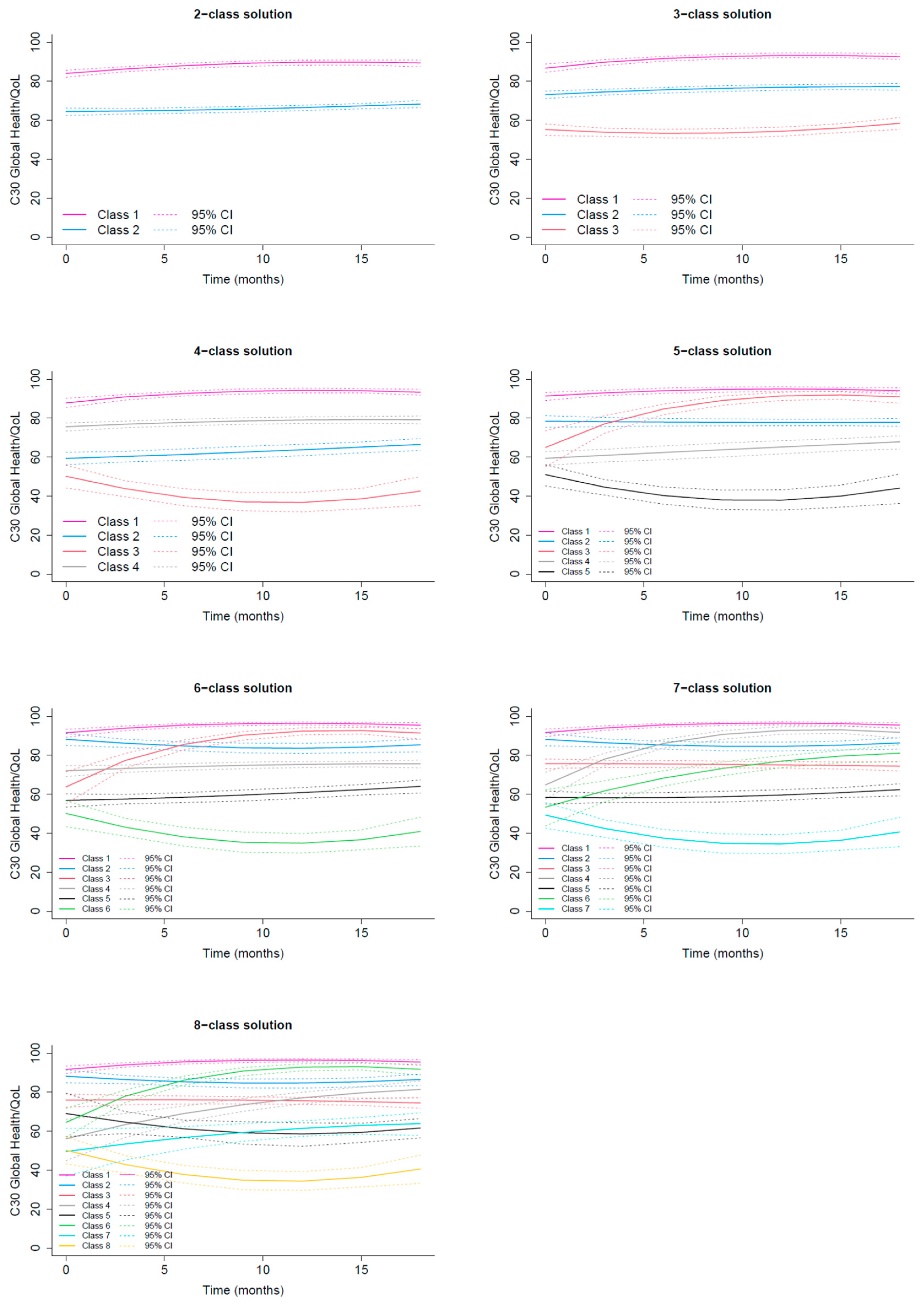
Figure B1. Estimated average C30 GHS/QoL trajectories for two- to eight-class solutions, shown for the LCGA approach.
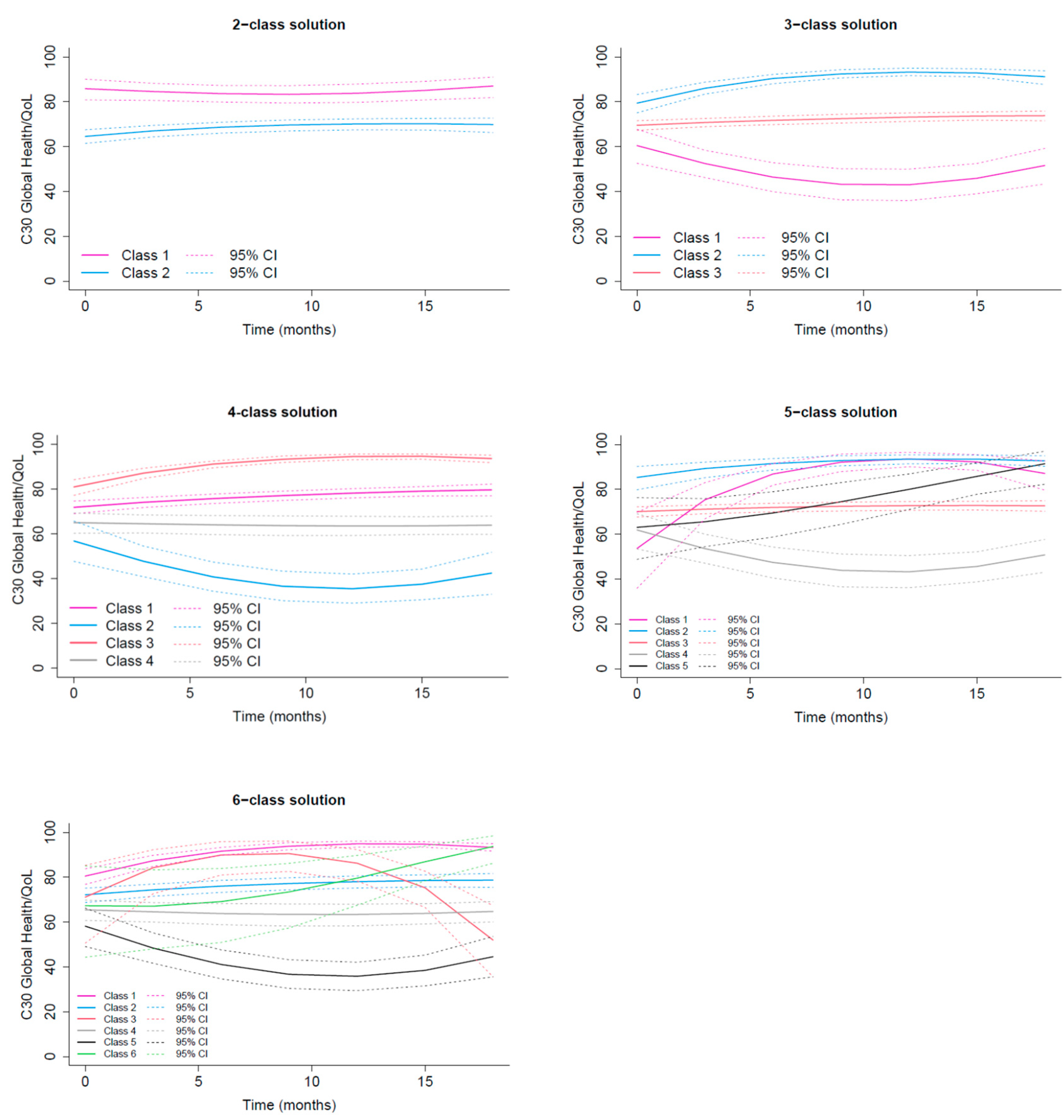
Figure B2. Estimated average C30 GHS/QoL trajectories for two- to eight-class solutions, shown for the GMM approach.
Appendix C
Trajectory Clustering of HADS Depression
The best-fitting LCGA model according to AIC and BIC is the eight-class solution, whereas ICL favors the six-class model (Table C1). However, in the five- to eight-class solutions, the smallest class comprises less than 5% of the sample, making these models unsuitable for further analysis.
In the two-, three- and four-class solutions, the classes exhibit very similar trajectory shapes (Figure C1). Their average trajectories remain largely steady over the 18-month period, with the exception of the class with the highest baseline depression scores, which shows a modest increase. Consequently, most trajectories are nearly parallel, differing primarily in baseline depression levels, all of which are below the clinically meaningful threshold of 1. From a clinical perspective, reassigning patients with depression scores below this threshold provides little added value.
Using the GMM approach, the best fitting model according to BIC and ICL is the null model, i.e. no latent classes, while the AIC indicates the six-class solution (Table C2). However, in the six- and five-class solutions, the size of the smallest class falls below 5% of the sample, making the four-class solution preferred choice. Classification quality of four-class model is acceptable, with posterior probabilities exceeding the 0.70 threshold for all classes.
Visual inspection of the four-class solution (Figure C2) reveals clinically meaningful trajectory patterns that were also present in solutions with a higher number of classes: two stable trajectories, one at low depression scores and one around a score of 1, as well as a low-worsening trajectory and an high-improving trajectory. Remarkably, the improving trajectory is also identified in the LCGA solutions with six or more classes.
Considering both statistical fit and clinical relevance, the four-class GMM solution was selected as optimal. This model encompassed all clinically important trajectory patterns while keeping class membership easily interpretable. Classification quality of the model is acceptable, with posterior probabilities exceeding 0.75 for all classes (Table C3).
Table C1. Goodness of fit statistics for HADS Depression LCGA model solutions and proportion of each class.
| No of classes | loglik | AIC | BIC | entropy | ICL | %class1 | %class2 | %class3 | %class4 | %class5 | %class6 | %class7 | %class8 |
| 1 | -1660 | 3341 | 3384 | 1 | 3384 | 100 | NA | NA | NA | NA | NA | NA | NA |
| 2 | -861 | 1750 | 1810 | 0.899 | 1848 | 47.21 | 52.79 | NA | NA | NA | NA | NA | NA |
| 3 | -631 | 1298 | 1375 | 0.873 | 1450 | 19.70 | 38.48 | 41.82 | NA | NA | NA | NA | NA |
| 4 | -553 | 1149 | 1243 | 0.845 | 1359 | 16.54 | 33.64 | 37.92 | 11.90 | NA | NA | NA | NA |
| 5 | -497 | 1047 | 1158 | 0.851 | 1287 | 3.53 | 37.17 | 17.47 | 30.67 | 11.15 | NA | NA | NA |
| 6 | -455 | 971 | 1099 | 0.843 | 1251 | 3.53 | 17.47 | 6.88 | 28.81 | 30.67 | 12.64 | NA | NA |
| 7 | -434 | 936 | 1082 | 0.798 | 1293 | 3.53 | 22.12 | 7.62 | 15.99 | 16.36 | 10.78 | 23.61 | NA |
| 8 | -412 | 900 | 1063 | 0.809 | 1277 | 2.60 | 7.62 | 23.05 | 1.12 | 23.79 | 10.59 | 15.61 | 15.61 |
| Note: AIC: Akaike Information Criterion; BIC: Bayesian Information Criterion; ICL: Integrated Complete Likelihood. | |||||||||||||
Table C2. Goodness of fit statistics for HADS Depression GMM model solutions and proportion of each class.
| Relative class size (%) | |||||||||||
| No of classes | loglik | AIC | BIC | entropy | ICL | %class1 | %class2 | %class3 | %class4 | %class5 | %class6 |
| 1 | -420 | 872 | 941 | 1 | 941 | 100 | NA | NA | NA | NA | NA |
| 2 | -410 | 860 | 946 | 0.586 | 1101 | 21.93 | 78.07 | NA | NA | NA | NA |
| 3 | -403 | 854 | 957 | 0.657 | 1159 | 2.60 | 23.79 | 73.61 | NA | NA | NA |
| 4 | -391 | 838 | 958 | 0.681 | 1196 | 10.04 | 5.02 | 59.67 | 25.28 | NA | NA |
| 5 | -383 | 829 | 966 | 0.732 | 1199 | 4.28 | 25.09 | 60.04 | 9.85 | 0.74 | NA |
| 6 | -373 | 819 | 973 | 0.772 | 1193 | 3.72 | 51.67 | 33.83 | 1.67 | 8.36 | 0.74 |
| Note: AIC: Akaike Information Criterion; BIC: Bayesian Information Criterion; ICL: Integrated Complete Likelihood. | |||||||||||
Table C3. Average of posterior probabilities in each class for HADS Depression GMM four-class solution.
| Assigned class | Class 1 Recovery | Class 2 Delayed occurrence | Class 3 Resilient | Class 4 Stable Moderate/High |
| 1 | 0.7735 | 0.0000 | 0.1608 | 0.0657 |
| 2 | 0.0000 | 0.7899 | 0.1206 | 0.0895 |
| 3 | 0.0375 | 0.0090 | 0.8620 | 0.0914 |
| 4 | 0.0353 | 0.0348 | 0.1760 | 0.7540 |
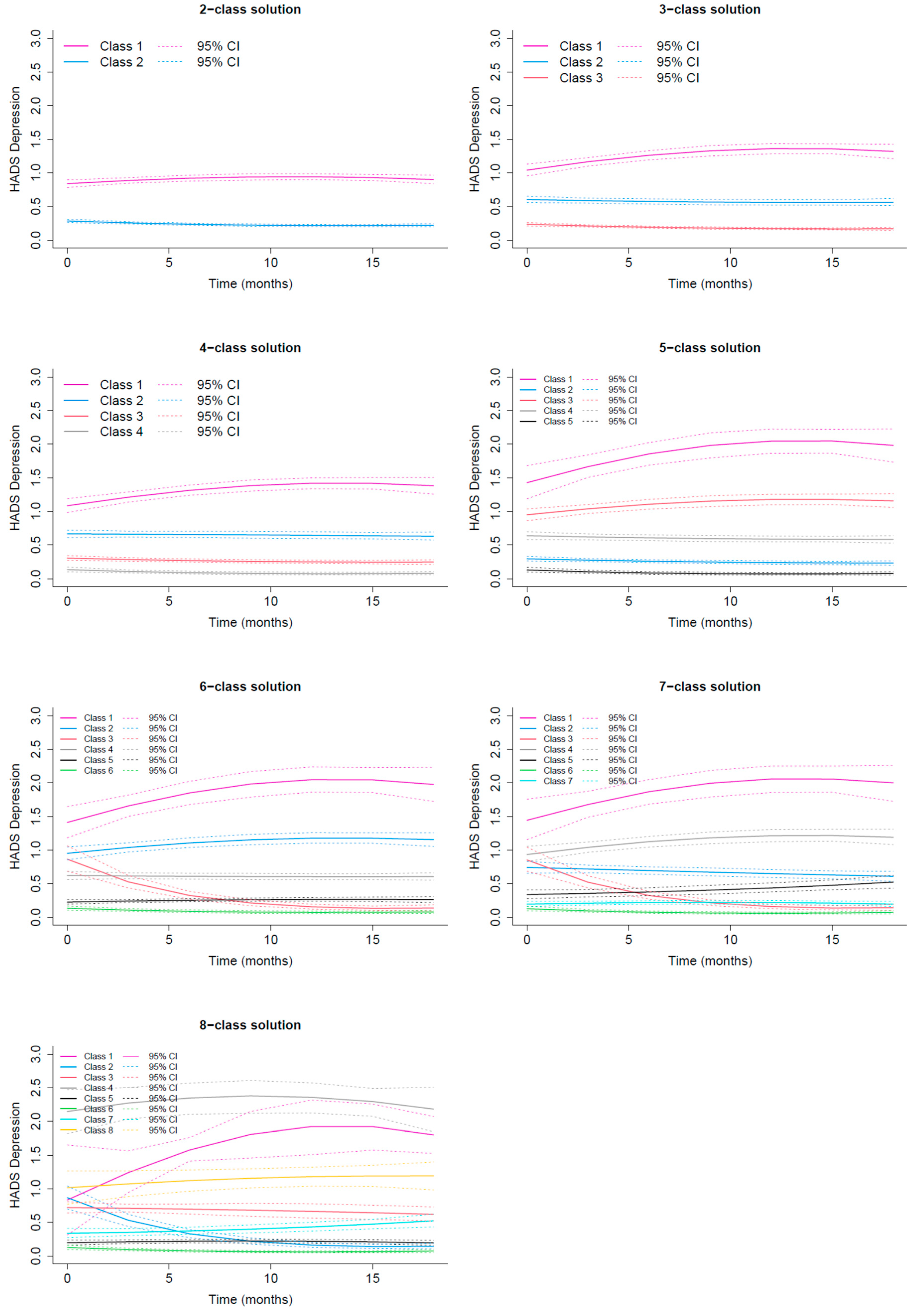
Figure C1. Estimated average HADS Depression trajectories for two- to eight-class solutions, shown for the LCGA approach.
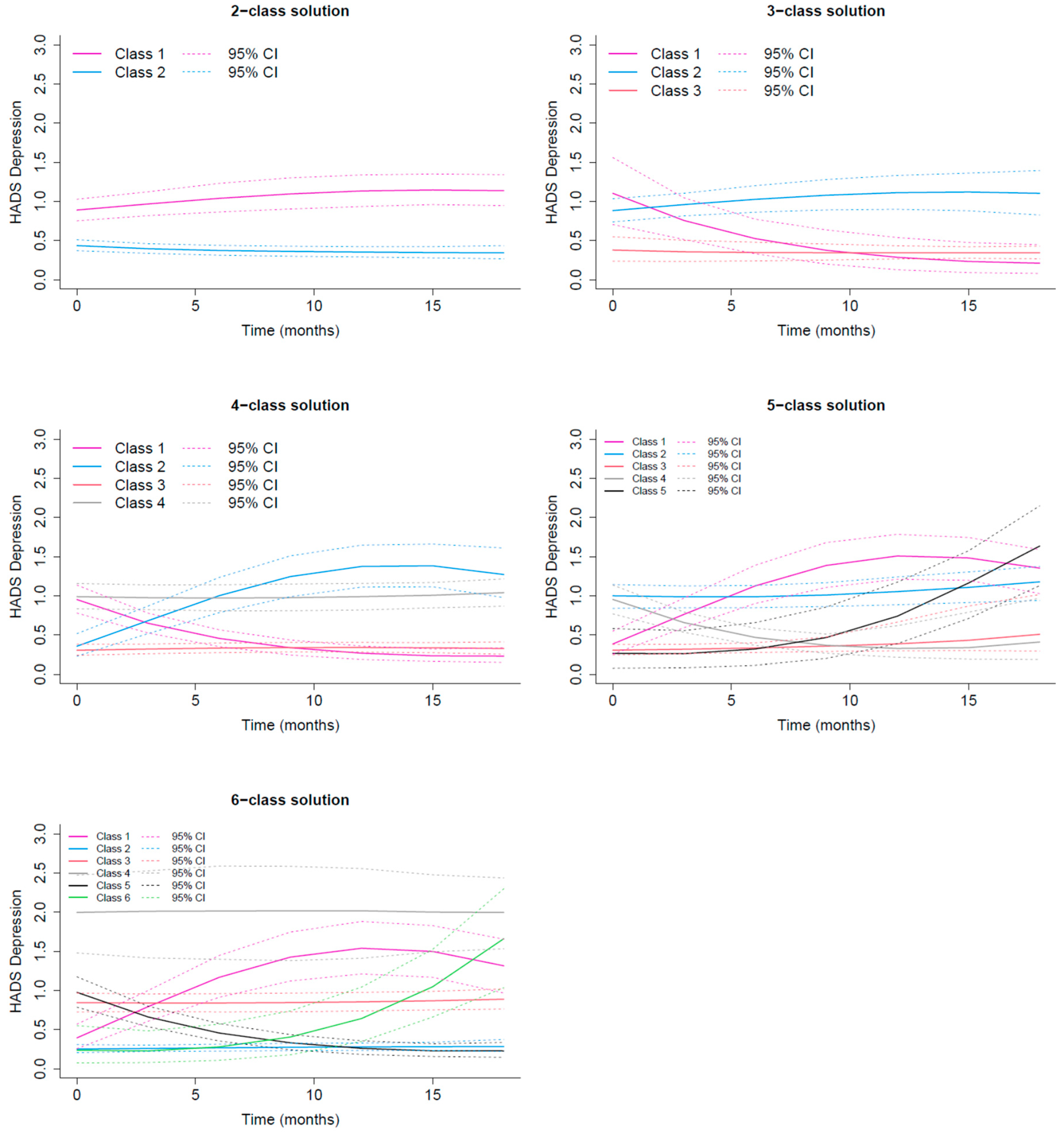
Figure C2. Estimated average HADS Depression trajectories for two- to six-class solutions, shown for the GMM approach.
Appendix D
Table D1. Maximum Likelihood Estimates for the selected C30 GHS/QoL five-class model. The Table presents estimated parameters, standard errors (SE), the Wald test statistics and corresponding p value. The Wald test assesses whether each parameter differs significantly from zero. Classes 1, 2, 3, 4 and 5 correspond to the Excellent, Good, Recovering, Moderate and Low deteriorating C30 GHS/QoL trajectory latent classes, respectively.
|
Fixed effects in the class-membership model: (the class of reference is the last class) | ||||
| coefficient | SE | Wald | p-value | |
| intercept class 1 | 0.55548 | 0.28801 | 1.929 | 0.05378 |
| intercept class 2 | 1.65476 | 0.30204 | 5.479 | 0.00000 |
| intercept class 3 | 0.10195 | 0.35111 | 0.290 | 0.77153 |
| intercept class 4 | 1.44951 | 0.23372 | 6.202 | 0.00000 |
| Fixed effects in the longitudinal model: | ||||
| coefficient | SE | Wald | p-value | |
| intercept class1 (not estimated) | 0 | |||
| intercept class 2 | -1.34743 | 0.18936 | -7.116 | 0.00000 |
| intercept class 3 | -2.39865 | 0.28857 | -8.312 | 0.00000 |
| intercept class 4 | -2.74885 | 0.18200 | -15.103 | 0.00000 |
| intercept class 5 | -3.26800 | 0.21464 | -15.226 | 0.00000 |
| linear slope class 1 | 0.09053 | 0.03134 | 2.889 | 0.00386 |
| linear slope class 2 | -0.00849 | 0.02040 | -0.416 | 0.67729 |
| linear slope class 3 | 0.34277 | 0.06492 | 5.280 | 0.00000 |
| linear slope class 4 | 0.03283 | 0.02206 | 1.488 | 0.13668 |
| linear slope class 5 | -0.13893 | 0.04217 | -3.295 | 0.00099 |
| quadratic slope class 1 | -0.00378 | 0.00164 | -2.305 | 0.02117 |
| quadratic slope class 2 | 0.00033 | 0.00101 | 0.329 | 0.74253 |
| quadratic slope class 3 | -0.01185 | 0.00300 | -3.945 | 0.00008 |
| quadratic slope class 4 | -0.00008 | 0.00116 | -0.070 | 0.94426 |
| quadratic slope class 5 | 0.00651 | 0.00222 | 2.934 | 0.00335 |
| Parameters of the link function: | ||||
| coefficient | SE | Wald | p-value | |
| I-splines 1 | -5.95455 | 0.21304 | -27.950 | 0.00000 |
| I-splines 2 | 1.06674 | 0.09931 | 10.742 | 0.00000 |
| I-splines 3 | 0.91341 | 0.09308 | 9.813 | 0.00000 |
| I-splines 4 | 1.42070 | 0.03349 | 42.424 | 0.00000 |
| I-splines 5 | 0.86157 | 0.02925 | 29.451 | 0.00000 |
| I-splines 6 | -1.17587 | 0.02114 | -55.617 | 0.00000 |
| I-splines 7 | 0.00011 | 0.03728 | 0.003 | 0.99767 |
| I-splines 8 | -0.95530 | 0.02128 | -44.889 | 0.00000 |
Table D2. Maximum Likelihood Estimates for the selected HADS Depression four-class model. The Table presents estimated parameters, standard errors (SE), the Wald test statistics and corresponding p value. The Wald test assesses whether each parameter differs significantly from zero. Classes 1, 2, 3 and 4 correspond to the Recovery, Delayed Occurrence, Resilient and Stable/High Depression trajectory latent classes, respectively.
|
Fixed effects in the class-membership model: (the class of reference is the last class) | ||||
| coefficient | SE | Wald | p-value | |
| intercept class 1 | -0.85515 | 0.34940 | -2.448 | 0.01438 |
| intercept class 2 | -1.56106 | 0.40570 | -3.848 | 0.00012 |
| intercept class 3 | 0.81867 | 0.29328 | 2.791 | 0.00525 |
| Fixed effects in the longitudinal model: | ||||
| coefficient | SE | Wald | p-value | |
| intercept class1 (not estimated) | 0 | |||
| intercept class 2 | -2.12840 | 0.43187 | -4.928 | 0.00000 |
| intercept class 3 | -2.40407 | 0.29120 | -8.256 | 0.00000 |
| intercept class 4 | 0.11938 | 0.33984 | 0.351 | 0.72537 |
| linear slope class 1 | -0.35787 | 0.05419 | -6.605 | 0.00000 |
| linear slope class 2 | 0.47814 | 0.07396 | 6.465 | 0.00000 |
| linear slope class 3 | 0.01588 | 0.02306 | 0.689 | 0.49109 |
| linear slope class 4 | -0.02495 | 0.03805 | -0.656 | 0.51200 |
| quadratic slope class 1 | 0.01082 | 0.00267 | 4.052 | 0.00005 |
| quadratic slope class 2 | -0.01737 | 0.00388 | -4.478 | 0.00001 |
| quadratic slope class 3 | -0.00075 | 0.00125 | -0.604 | 0.54560 |
| quadratic slope class 4 | 0.00171 | 0.00216 | 0.792 | 0.42858 |
| Variance-covariance matrix of the random-effects: | ||||
| intercept | linear slope | quadratic slope | ||
| intercept | 0.89100 | |||
| linear slope | 0.03042 | 0.00566 | ||
| quadratic slope | -0.00159 | -0.00025 | 1e-05 | |
| Parameters of the link function: | ||||
| coefficient | SE | Wald | p-value | |
| I-splines 1 | -4.61362 | 0.28054 | -16.446 | 0.00000 |
| I-splines 2 | 0.95180 | 0.02099 | 45.347 | 0.00000 |
| I-splines 3 | 0.79402 | 0.03608 | 22.006 | 0.00000 |
| I-splines 4 | 1.17562 | 0.02950 | 39.851 | 0.00000 |
| I-splines 5 | 0.93434 | 0.03303 | 28.292 | 0.00000 |
| I-splines 6 | 1.61728 | 0.04373 | 36.986 | 0.00000 |
| I-splines 7 | 1.24502 | 0.11248 | 11.069 | 0.00000 |
| I-splines 8 | 1.15337 | 0.13638 | 8.457 | 0.00000 |
References
- Pravettoni, G.; Gorini, A. A P5 cancer medicine approach: why personalized medicine cannot ignore psychology. Evaluation Clinical Practice 2011, 17, 594–596. [Google Scholar] [CrossRef]
- Bonanno, G.A.; Galea, S.; Bucciarelli, A.; Vlahov, D. What predicts psychological resilience after disaster? The role of demographics, resources, and life stress. J Consult Clin Psychol. 2007, 75, 671–682. [Google Scholar] [CrossRef]
- Carver, C.S. Enhancing adaptation during treatment and the role of individual differences. Cancer 2005, 104, 2602–2607. [Google Scholar] [CrossRef]
- Molina, Y.; Yi, J.C.; Martinez-Gutierrez, J.; Reding, K.W.; Yi-Frazier, J.P.; Rosenberg, A.R. Resilience Among Patients Across the Cancer Continuum: Diverse Perspectives. Clinical Journal of Oncology Nursing 2014, 18, 93–101. [Google Scholar] [CrossRef]
- Garnefski, N.; Kraaij, V.; Spinhoven, P. Negative life events, cognitive emotion regulation and emotional problems. Personality and Individual Differences 2001, 30, 1311–1327. [Google Scholar] [CrossRef]
- Li, L.; Zhu, X.; Yang, Y.; et al. Cognitive emotion regulation: characteristics and effect on quality of life in women with breast cancer. Health Qual Life Outcomes 2015, 13, 51. [Google Scholar] [CrossRef]
- Hamama-Raz, Y.; Pat-Horenczyk, R.; Perry, S.; Ziv, Y.; Bar-Levav, R.; Stemmer, S.M. The Effectiveness of Group Intervention on Enhancing Cognitive Emotion Regulation Strategies in Breast Cancer Patients: A 2-Year Follow-up. Integr Cancer Ther. 2016, 15, 175–182. [Google Scholar] [CrossRef] [PubMed]
- Nolen-Hoeksema, S.; Aldao, A. Gender and age differences in emotion regulation strategies and their relationship to depressive symptoms. Personality and Individual Differences 2011, 51, 704–708. [Google Scholar] [CrossRef]
- Wang, Y.; Yi, J.; He, J.; et al. Cognitive emotion regulation strategies as predictors of depressive symptoms in women newly diagnosed with breast cancer: Cognitive strategies predict depression in women with breast cancer. Psycho-Oncology 2014, 23, 93–99. [Google Scholar] [CrossRef] [PubMed]
- Mazzocco, K.; Masiero, M.; Carriero, M.C.; Pravettoni, G. The role of emotions in cancer patients’ decision-making. ecancer 2019, 13. [Google Scholar] [CrossRef]
- Gorini, A.; Riva, S.; Marzorati, C.; Cropley, M.; Pravettoni, G. Rumination in breast and lung cancer patients: Preliminary data within an Italian sample. Psycho-Oncology 2018, 27, 703–705. [Google Scholar] [CrossRef]
- Novakov, I.; Popovic-Petrovic, S. Personality traits as predictors of the affective state in patients after breast cancer surgery. Arch Oncol. 2017, 23, 3–8. [Google Scholar] [CrossRef]
- Exploring the Role of Self-Efficacy for Coping With Breast Cancer: A Systematic Review. Archives of Breast Cancer 2017, 42–57. [CrossRef]
- Wills, T.A.; Bantum, E.O. Social Support, Self-Regulation, and Resilience in Two Populations: General-Population Adolescents and Adult Cancer Survivors. Journal of Social and Clinical Psychology 2012, 31, 568–592. [Google Scholar] [CrossRef]
- Rolland, J.S. Cancer and the family: An integrative model. Cancer 2005, 104, 2584–2595. [Google Scholar] [CrossRef] [PubMed]
- Faccio, F.; Gandini, S.; Renzi, C.; Fioretti, C.; Crico, C.; Pravettoni, G. Development and validation of the Family Resilience (FaRE) Questionnaire: an observational study in Italy. BMJ Open. 2019, 9, e024670. [Google Scholar] [CrossRef] [PubMed]
- Faccio, F.; Renzi, C.; Giudice, A.V.; Pravettoni, G. Family Resilience in the Oncology Setting: Development of an Integrative Framework. Front Psychol. 2018, 9, 666. [Google Scholar] [CrossRef]
- Pettini, G.; Sanchini, V.; Pat-Horenczyk, R.; et al. Predicting Effective Adaptation to Breast Cancer to Help Women BOUNCE Back: Protocol for a Multicenter Clinical Pilot Study. JMIR Res Protoc. 2022, 11, e34564. [Google Scholar] [CrossRef]
- Mitchell, A.J.; Meader, N.; Symonds, P. Diagnostic validity of the Hospital Anxiety and Depression Scale (HADS) in cancer and palliative settings: A meta-analysis. Journal of Affective Disorders 2010, 126, 335–348. [Google Scholar] [CrossRef]
- Wu, Y.; Levis, B.; Sun, Y.; et al. Accuracy of the Hospital Anxiety and Depression Scale Depression subscale (HADS-D) to screen for major depression: systematic review and individual participant data meta-analysis. BMJ 2021, n972. [Google Scholar] [CrossRef]
- Puhan, M.A.; Frey, M.; Büchi, S.; Schünemann, H.J. The minimal important difference of the hospital anxiety and depression scale in patients with chronic obstructive pulmonary disease. Health Qual Life Outcomes 2008, 6, 46. [Google Scholar] [CrossRef]
- Vaganian, L.; Bussmann, S.; Gerlach, A.L.; Kusch, M.; Labouvie, H.; Cwik, J.C. Critical consideration of assessment methods for clinically significant changes of mental distress after psycho-oncological interventions. Int J Methods Psych Res. 2020, 29, e1821. [Google Scholar] [CrossRef]
- Longo, U.G.; Papalia, R.; De Salvatore, S.; et al. Establishing the Minimum Clinically Significant Difference (MCID) and the Patient Acceptable Symptom Score (PASS) for the Hospital Anxiety and Depression Scale (HADS) in Patients with Rotator Cuff Disease and Shoulder Prosthesis. JCM 2023, 12, 1540. [Google Scholar] [CrossRef]
- Karsten, M.M.; Roehle, R.; Albers, S.; et al. Real-world reference scores for EORTC QLQ-C30 and EORTC QLQ-BR23 in early breast cancer patients. European Journal of Cancer 2022, 163, 128–139. [Google Scholar] [CrossRef]
- Saini, J.; Bakshi, J.; Panda, N.K.; Sharma, M.; Vir, D.; Goyal, A.K. Cut-off points to classify numeric values of quality of life into normal, mild, moderate, and severe categories: an update for EORTC-QLQ-H&N35. Egypt J Otolaryngol. 2024, 40, 83. [Google Scholar] [CrossRef]
- Diouf, M.; Bonnetain, F.; Barbare, J.C.; et al. Optimal Cut Points for Quality of Life Questionnaire-Core 30 (QLQ-C30) Scales: Utility for Clinical Trials and Updates of Prognostic Systems in Advanced Hepatocellular Carcinoma. The Oncologist 2015, 20, 62–71. [Google Scholar] [CrossRef]
- Snyder, C.F.; Blackford, A.L.; Sussman, J.; et al. Identifying changes in scores on the EORTC-QLQ-C30 representing a change in patients’ supportive care needs. Qual Life Res. 2015, 24, 1207–1216. [Google Scholar] [CrossRef] [PubMed]
- Scheier, M.F.; Carver, C.S.; Bridges, M.W. Distinguishing optimism from neuroticism (and trait anxiety, self-mastery, and self-esteem): A reevaluation of the Life Orientation Test. Journal of Personality and Social Psychology 1994, 67, 1063–1078. [Google Scholar] [CrossRef] [PubMed]
- Antonovsky, A. The structure and properties of the sense of coherence scale. Social Science & Medicine 1993, 36, 725–733. [Google Scholar] [CrossRef]
- Connor, K.M.; Davidson, J.R.T. Development of a new resilience scale: The Connor-Davidson Resilience Scale (CD-RISC). Depress Anxiety 2003, 18, 76–82. [Google Scholar] [CrossRef] [PubMed]
- Carlson, L.E.; Brown, K.W. Validation of the Mindful Attention Awareness Scale in a cancer population. Journal of Psychosomatic Research 2005, 58, 29–33. [Google Scholar] [CrossRef]
- Bonanno, G.A.; Pat-Horenczyk, R.; Noll, J. Coping flexibility and trauma: The Perceived Ability to Cope With Trauma (PACT) scale. Psychological Trauma: Theory, Research, Practice, and Policy 2011, 3, 117–129. [Google Scholar] [CrossRef]
- Heitzmann, C.A.; Merluzzi, T.V.; Jean-Pierre, P.; Roscoe, J.A.; Kirsh, K.L.; Passik, S.D. Assessing self-efficacy for coping with cancer: development and psychometric analysis of the brief version of the Cancer Behavior Inventory (CBI-B). Psycho-Oncology 2011, 20, 302–312. [Google Scholar] [CrossRef]
- Simard, S.; Savard, J. Screening and comorbidity of clinical levels of fear of cancer recurrence. J Cancer Surviv. 2015, 9, 481–491. [Google Scholar] [CrossRef]
- Watson, M.; Law, M.G.; Santos, M.D.; Greer, S.; Baruch, J.; Bliss, J. The Mini-MAC: Further Development of the Mental Adjustment to Cancer Scale. Journal of Psychosocial Oncology 1994, 12, 33–46. [Google Scholar] [CrossRef]
- Cann, A.; Calhoun, L.G.; Tedeschi, R.G.; et al. A short form of the Posttraumatic Growth Inventory. Anxiety, Stress & Coping 2010, 23, 127–137. [Google Scholar] [CrossRef]
- Watson, D.; Clark, L.A.; Tellegen, A. Development and validation of brief measures of positive and negative affect: The PANAS scales. Journal of Personality and Social Psychology 1988, 54, 1063–1070. [Google Scholar] [CrossRef]
- Moser, A.; Stuck, A.E.; Silliman, R.A.; Ganz, P.A.; Clough-Gorr, K.M. The eight-item modified Medical Outcomes Study Social Support Survey: psychometric evaluation showed excellent performance. Journal of Clinical Epidemiology 2012, 65, 1107–1116. [Google Scholar] [CrossRef] [PubMed]
- Buuren, S.V.; Groothuis-Oudshoorn, K. mice : Multivariate Imputation by Chained Equations in R. J Stat Soft 2011, 45. [Google Scholar] [CrossRef]
- Proust-Lima, C.; Philipps, V.; Liquet, B. Estimation of Extended Mixed Models Using Latent Classes and Latent Processes: The R Package lcmm. J Stat Soft 2017, 78. [Google Scholar] [CrossRef]
- Van De Schoot, R.; Sijbrandij, M.; Winter, S.D.; Depaoli, S.; Vermunt, J.K. The GRoLTS-Checklist: Guidelines for Reporting on Latent Trajectory Studies. Structural Equation Modeling: A Multidisciplinary Journal 2017, 24, 451–467. [Google Scholar] [CrossRef]
- Weller, B.E.; Bowen, N.K.; Faubert, S.J. Latent Class Analysis: A Guide to Best Practice. Journal of Black Psychology 2020, 46, 287–311. [Google Scholar] [CrossRef]
- Van Der Nest, G.; Lima Passos, V.; Candel, M.J.J.M.; Van Breukelen, G.J.P. An overview of mixture modelling for latent evolutions in longitudinal data: Modelling approaches, fit statistics and software. Advances in Life Course Research 2020, 43, 100323. [Google Scholar] [CrossRef]
- Tay, J.K.; Narasimhan, B.; Hastie, T. Elastic Net Regularization Paths for All Generalized Linear Models. J Stat Soft 2023, 106. [Google Scholar] [CrossRef]
- Zou, H.; Hastie, T. Regularization and Variable Selection Via the Elastic Net. Journal of the Royal Statistical Society Series B: Statistical Methodology 2005, 67, 301–320. [Google Scholar] [CrossRef]
- Hastie, T.; Tibshirani, R.; Friedman, J.H. The Elements of Statistical Learning: Data Mining, Inference, and Prediction, Second edition; Springer, 2017. [Google Scholar]
- Hosmer, D.W.; Lemeshow, S.; Sturdivant, R.X. Applied Logistic Regression, 1st ed.; Wiley, 2013. [Google Scholar] [CrossRef]
- Park, J.H.; Jung, Y.S.; Kim, J.Y.; Bae, S.H. Trajectories of quality of life in breast cancer survivors during the first year after treatment: a longitudinal study. BMC Women’s Health 2023, 23, 12. [Google Scholar] [CrossRef]
- Di Meglio, A.; Havas, J.; Gbenou, A.S.; et al. Dynamics of Long-Term Patient-Reported Quality of Life and Health Behaviors After Adjuvant Breast Cancer Chemotherapy. JCO 2022, 40, 3190–3204. [Google Scholar] [CrossRef] [PubMed]
- Goyal, N.G.; Levine, B.J.; Van Zee, K.J.; Naftalis, E.; Avis, N.E. Trajectories of quality of life following breast cancer diagnosis. Breast Cancer Res Treat. 2018, 169, 163–173. [Google Scholar] [CrossRef] [PubMed]
- Charles, C.; Bardet, A.; Larive, A.; et al. Characterization of Depressive Symptoms Trajectories After Breast Cancer Diagnosis in Women in France. JAMA Netw Open. 2022, 5, e225118. [Google Scholar] [CrossRef]
- Kant, J.; Czisch, A.; Schott, S.; Siewerdt-Werner, D.; Birkenfeld, F.; Keller, M. Identifying and predicting distinct distress trajectories following a breast cancer diagnosis - from treatment into early survival. Journal of Psychosomatic Research 2018, 115, 6–13. [Google Scholar] [CrossRef]
- Li, W.; Zhang, Q.; Xu, Y.; et al. Group-based trajectory and predictors of anxiety and depression among Chinese breast cancer patients. Front Public Health 2022, 10, 1002341. [Google Scholar] [CrossRef]
- Karademas, E.C.; Mylona, E.; Mazzocco, K.; et al. Well-being trajectories in breast cancer and their predictors: A machine-learning approach. Psycho-Oncology 2023, 32, 1762–1770. [Google Scholar] [CrossRef]
- Genolini, C.; Ecochard, R.; Benghezal, M.; Driss, T.; Andrieu, S.; Subtil, F. kmlShape: An Efficient Method to Cluster Longitudinal Data (Time-Series) According to Their Shapes. PLoS One 2016, 11, e0150738. [Google Scholar] [CrossRef]
- Strobl, C.; Boulesteix, A.L.; Zeileis, A.; Hothorn, T. Bias in random forest variable importance measures: Illustrations, sources and a solution. BMC Bioinformatics 2007, 8, 25. [Google Scholar] [CrossRef] [PubMed]
- Den Teuling, N.; Pauws, S.; Van Den Heuvel, E. latrend: A Framework for Clustering Longitudinal Data. The R Journal. 2025, 17, 108–135. [Google Scholar] [CrossRef]
- Verboon, P.; Pat-El, R. Clustering longitudinal data using R: A Monte Carlo Study. Published online. 30 June 2022. [CrossRef]
- Lu, Z.; Ahmadiankalati, M.; Tan, Z. Joint clustering multiple longitudinal features: A comparison of methods and software packages with practical guidance. Statistics in Medicine 2023, 42, 5513–5540. [Google Scholar] [CrossRef]
- Martin, D.P.; Von Oertzen, T. Growth Mixture Models Outperform Simpler Clustering Algorithms When Detecting Longitudinal Heterogeneity, Even With Small Sample Sizes. Structural Equation Modeling: A Multidisciplinary Journal. 2015, 22, 264–275. [Google Scholar] [CrossRef]
- Hong, J.E.; Kim, Y.E.; Kang, Y.S.; Choi, D.H.; Ahn, S.H.; An, J. SMOTE-augmented machine learning model predicts recurrent and metastatic breast cancer from microbiome analysis. Sci Rep. 2025, 15, 33096. [Google Scholar] [CrossRef]
- Tran, T.; Le, U.; Shi, Y. An effective up-sampling approach for breast cancer prediction with imbalanced data: A machine learning model-based comparative analysis. In PLoS ONE; E S, V, Ed.; 2022; Volume 17. [Google Scholar] [CrossRef]
- Rudin, C. Stop explaining black box machine learning models for high stakes decisions and use interpretable models instead. Nat Mach Intell. 2019, 1, 206–215. [Google Scholar] [CrossRef]
- Sarica, A.; Aracri, F.; Bianco, M.G.; et al. Explainability of random survival forests in predicting conversion risk from mild cognitive impairment to Alzheimer’s disease. Brain Inf. 2023, 10, 31. [Google Scholar] [CrossRef] [PubMed]
- Angelopoulos, A.N.; Bates, S. Conformal Prediction: A Gentle Introduction. Foundations and Trends in Machine Learning 2023, 16, 494–591. [Google Scholar] [CrossRef]
- Alnemer, L.M.; Rajab, L.; Aljarah, I. Conformal Prediction Technique to Predict Breast Cancer Survivability. IJAST 2016, 96, 1–10. [Google Scholar] [CrossRef]
- Sreenivasan, A.P.; Vaivade, A.; Noui, Y.; et al. Conformal prediction enables disease course prediction and allows individualized diagnostic uncertainty in multiple sclerosis. npj Digit Med. 2025, 8, 224. [Google Scholar] [CrossRef] [PubMed]
Figure 1.
Mean growth trajectories and observed individual patient trajectories, grouped by trajectory latent classes for (a) EORTC QLQ-C30 Global Health Status/Quality of Life scores and (b) HADS Depression scores.
Figure 1.
Mean growth trajectories and observed individual patient trajectories, grouped by trajectory latent classes for (a) EORTC QLQ-C30 Global Health Status/Quality of Life scores and (b) HADS Depression scores.
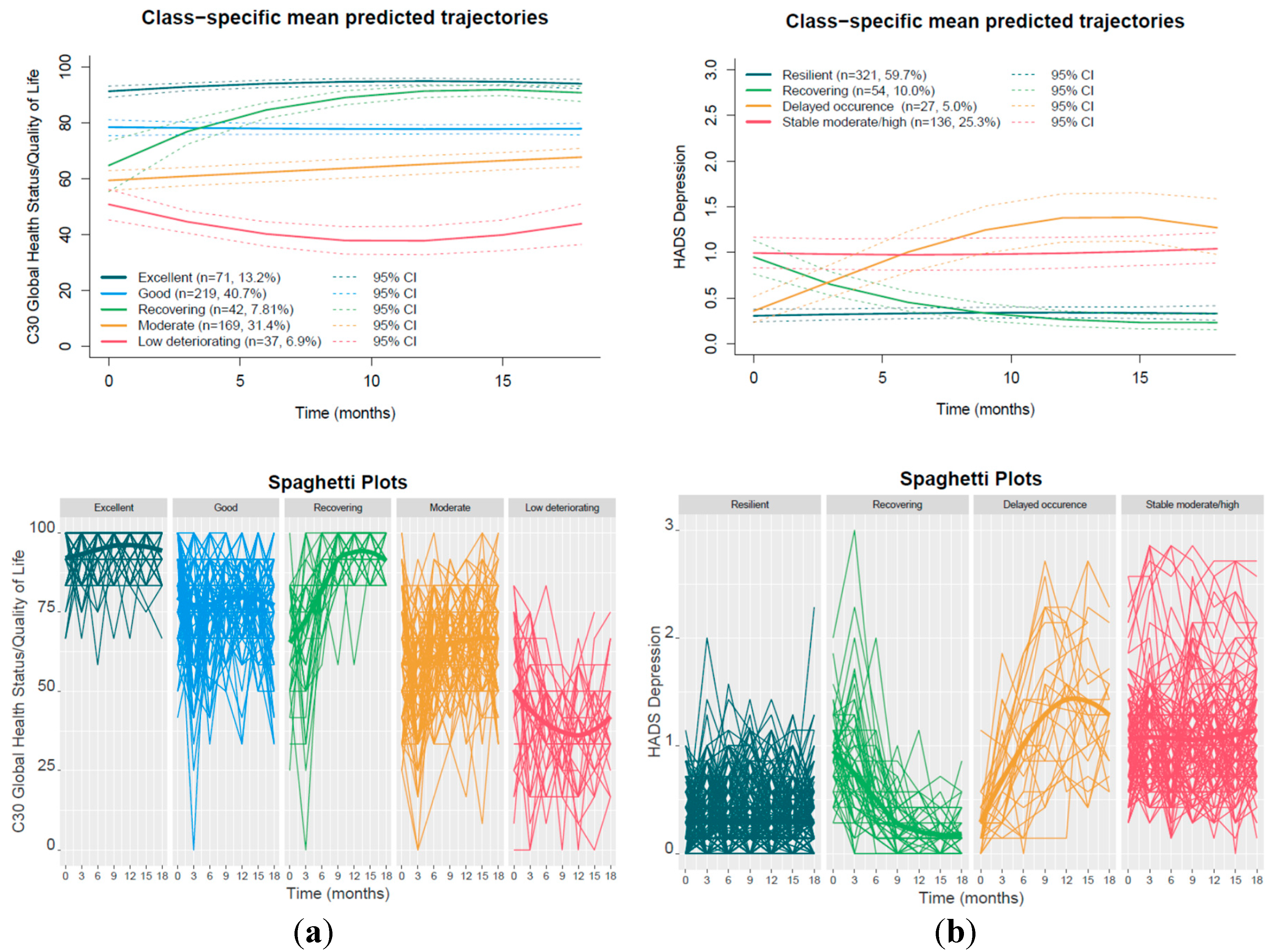
Table 1.
Baseline sociodemographic and lifestyle characteristics of the study participants. Total number of patients n=538.
Table 1.
Baseline sociodemographic and lifestyle characteristics of the study participants. Total number of patients n=538.
| Variable | Mean (range) | Variable | n (%) |
|---|---|---|---|
| Age | 55.4 (40-70) | Monthly Income 1 | |
| BMI | 26 (17.3-54.1) | Low | 103 (20.2%) |
| Variable | n (%) | Middle | 315 (61.6%) |
| Country/Clinical site | High | 93 (18.2%) | |
| Portugal | 134 (24.9%) | Exercise level2 | |
| Italy | 95 (17.7%) | None | 166 (33.7%) |
| Finland | 205 (38.1%) | Low/moderate | 179 (36.4%) |
| Israel | 104 (19.3%) | Heavy | 147 (29.9%) |
| Education | Diet | ||
| Non University | 211 (39.3%) | No diet | 293 (54.6%) |
| University | 326 (60.7%) | Mediterranean/Vegetarian type | 166 (30.9%) |
| Marital status | Special | 78 (14.5%) | |
| Single/Engaged | 53 (9.9%) | Alcohol behavior3 | |
| Married/Common in Law | 400 (74.9%) | No Consumption | 107 (22.1%) |
| Divorced/Widowed | 81 (15.2%) | Consumption in Moderation | 331 (68.2%) |
| Employment status | Heavy Consumption | 47 (9.7%) | |
| Full/part- time/Self-employed | 390 (72.9%) | Smoking behavior | |
| Unemployed/Housewife | 47 (8.8%) | Current smoker | 72 (13.5%) |
| Retired | 98 (18.3%) | Never smoker | 359 (67.4%) |
| Former smoker | 102 (19.1%) |
1Low monthly income was defined as ≤1,000 EUR for the moderate-income countries (Portugal, Italy) and ≤1,500 EUR for the higher-income countries (Finland, Israel). High monthly income was defined as >3,000 EUR (Portugal, Italy) or >3,500 EUR (Finland, Israel). 2Heavy exercise was defined as ≥200 min/week moderate or ≥100 min/week vigorous aerobic activity and combinations. Moderate aerobic activity includes walking, cycling and similar activities, while vigorous aerobic activity includes running, HIIT training and comparable high-intensity exercises. 3Heavy alcohol consumption was defined as consuming more than 3 drinks on any day or more than 7 drinks per week.
Table 3.
Stability-selected predictors distinguishing the low deteriorating QoL trajectory from all other trajectory classes with descriptive penalized odds ratios.
Table 3.
Stability-selected predictors distinguishing the low deteriorating QoL trajectory from all other trajectory classes with descriptive penalized odds ratios.
| Variable | Selection Freq (%) Penalized Site |
Mean OR1 Penalized Site |
Selection Freq (%) Unpenalized Site |
|---|---|---|---|
| Baseline | |||
| Performance2: log-loss = 0.191, Brier score = 0.052, ROC-AUC = 0.855 | |||
| Depression HADS | 100% | 1.4081 | 100% |
| Diarrhea C30 | 100% | 1.004 | 100% |
| Emotional functioning C30 | 100% | 0.9976 | 100% |
| Fatigue C30 | 100% | 1.0011 | 100% |
| GHS/QoL C30 | 100% | 0.9857 | 100% |
| Coping with cancer CBI | 100% | 0.9623 | 97% |
| Manageability SOC | 100% | 0.9548 | 100% |
| Other blame CERQ | 100% | 1.2173 | 100% |
| Pain C30 | 100% | 1.0154 | 100% |
| Neoadjuvant Chemotherapy | 100% | 1.4209 | 83% |
| Perceived support 1 item | 100% | 0.8896 | 100% |
| Triple−negative | 83% | 1.429 | 60% |
| Negative Life Events: Two or more (ref. No) | 67% | 1.0899 | 57% |
| Month 33 | |||
| Performance2: log-loss = 0.196, Brier score = 0.0537, ROC-AUC = 0.855 | |||
| Cognitive Function C30 | 100% | 0.9924 | 100% |
| Depression HADS | 100% | 1.8171 | 100% |
| Physical Function C30 | 100% | 0.9875 | 100% |
| Treatment control beliefs | 100% | 0.9005 | 100% |
| Anxiety HADS | 90% | 1.1226 | 87% |
| Neoadjuvant Chemotherapy | 73% | 1.1347 | 27% |
| Communication and cohesion FARE | 70% | 0.9455 | 73% |
1 Penalized odds ratios are descriptive estimates from elastic net models at the selected λ and are not directly comparable due to differences in variable scaling. 2 The performance of the model when clinical site is penalized, i.e. not forced into the model. 3 GHS/QoL C30 was not included in the variables at month 3.
Table 4.
Stability-selected predictors distinguishing the excellent QoL trajectory (reference) from all other trajectory classes, with descriptive penalized odds ratios.
Table 4.
Stability-selected predictors distinguishing the excellent QoL trajectory (reference) from all other trajectory classes, with descriptive penalized odds ratios.
| Variable | Selection Freq (%) Penalized Site |
Mean OR1 Penalized Site |
Selection Freq (%) Unpenalized Site |
|---|---|---|---|
| Baseline | |||
| Performance2: log-loss = 0.276, Brier score = 0.0852, ROC-AUC = 0.879 | |||
| Anxiety HADS | 100% | 0.8796 | 93% |
| Cognitive functioning C30 | 100% | 1.0059 | 100% |
| Constipation C30 | 100% | 0.998 | 100% |
| Emotional functioning C30 | 100% | 1.0068 | 100% |
| Mental illness (ref. No) | 100% | 0.8947 | 10% |
| Fatigue C30 | 100% | 0.9955 | 100% |
| GHS/QoL C30 | 100% | 1.0501 | 100% |
| Mindfulness MAAS | 100% | 1.224 | 100% |
| Resilience CDRISC | 100% | 1.2044 | 100% |
| Self blame CERQ | 100% | 0.8493 | 100% |
| Physical functioning C30 | 100% | 1.0106 | 100% |
| Role functioning | 100% | 1.0029 | 100% |
| Luminal A-like | 100% | 1.3491 | 100% |
| Israel (ref.Portugal) | 100% | 1.1341 | - |
| Endocrine only (ref. Chemo only +/−Anti−HER2) | 100% | 1.107 | 63% |
| Mediterranean/Vegetarian diet (ref. None) | 100% | 0.9513 | 70% |
| Unemployed/Housewife (ref. Full/part− time/Self−employed) | 100% | 0.9384 | 100% |
| Neoadjuvant Chemotherapy | 100% | 0.7816 | 100% |
| Perceived support 1 item | 100% | 1.0287 | 97% |
| Future Perspective Image BR23 | 97% | 1.0014 | 97% |
| Meaningfulness SOC | 93% | 1.0026 | 80% |
| Positive affect PANAS | 93% | 1.014 | 0% |
| General self−efficacy 1 item | 93% | 1.0907 | 90% |
| Arm Symptoms BR23 | 90% | 0.9991 | 100% |
| Distress thermometer NCCN | 90% | 0.9624 | 90% |
| Coping with cancer CBI | 87% | 1.0278 | 100% |
| Luminal B-like (HER2 +) | 83% | 0.9583 | 63% |
| Catastrophizing CERQ | 80% | 0.9764 | 97% |
| Negative Life Events: Two or more (ref. No) | 77% | 0.9199 | 77% |
| Month 33 | |||
| Performance2: log-loss = 0.306, Brier score = 0.0928, ROC-AUC = 0.845 | |||
| Anxiety HADS | 100% | 0.744 | 100% |
| Fatigue C30 | 100% | 0.988 | 100% |
| Anxious preoccupation MAC | 100% | 0.8719 | 100% |
| Positive affect PANAS | 100% | 1.3538 | 100% |
| Role functioning | 100% | 1.0055 | 100% |
| Systemic Therapy Side Effects BR23 | 100% | 0.9963 | 100% |
| Social functioning | 100% | 1.004 | 100% |
| Personal control beliefs over illness | 100% | 1.0147 | 80% |
| Distress thermometer NCCN | 100% | 0.9693 | 97% |
| What done to cope: Talked to the physician | 100% | 0.9495 | 97% |
| Future Perspective Image BR23 | 97% | 1.0027 | 97% |
| Depression HADS | 93% | 0.8901 | 80% |
| Negative affect PANAS | 93% | 0.9418 | 13% |
| Physical functioning C30 | 93% | 1.003 | 97% |
| Perceived support 1 item | 93% | 1.0361 | 90% |
| Arm Symptoms BR23 | 90% | 0.9974 | 90% |
| Emotional functioning C30 | 83% | 1.003 | 87% |
| Communication and cohesion FARE | 77% | 1.0215 | 83% |
| Pain C30 | 77% | 0.9962 | 83% |
| Emotional support mMOS | 73% | 1.0395 | 67% |
| Negative Life Events: Two or more (ref. No) | 70% | 0.916 | 83% |
1 Penalized odds ratios are descriptive estimates from elastic net models at the selected λ and are not directly comparable due to differences in variable scaling. 2 The performance of the model when clinical site is penalized, i.e. not forced into the model. 3 GHS/QoL C30 was not included in the variables at month 3.
Table 5.
Stability-selected predictors distinguishing the moderate QoL trajectory from the recovering QoL trajectory (reference), with descriptive penalized odds ratios.
Table 5.
Stability-selected predictors distinguishing the moderate QoL trajectory from the recovering QoL trajectory (reference), with descriptive penalized odds ratios.
| Variable | Selection Freq (%) Penalized Site |
Mean OR1 Penalized Site |
Selection Freq (%) Unpenalized Site |
|---|---|---|---|
| Baseline | |||
| Performance2: log-loss = 0.464, Brier score = 0.147, ROC-AUC = 0.681 | |||
| Coping with cancer CBI | 100% | 1.0568 | 97% |
| Mindfulness MAAS | 100% | 1.0276 | 93% |
| Optimism LOT | 100% | 1.1892 | 100% |
| Perspective CERQ | 100% | 1.0756 | 90% |
| Resilience CDRISC | 100% | 1.0604 | 0% |
| Pain C30 | 100% | 0.9978 | 100% |
| Positive affect PANAS | 100% | 1.0919 | 100% |
| Sexual functioning BR23 | 100% | 1.0033 | 90% |
| Social functioning C30 | 100% | 1.0047 | 100% |
| Income Middle (ref. Low) | 100% | 0.7621 | 97% |
| Income High (ref. Low) | 100% | 1.5861 | 100% |
| Postmenopausal | 93% | 1.0937 | 17% |
| Planning CERQ | 90% | 1.0193 | 70% |
| Negative Life Events: Two or more (ref. No) | 80% | 0.9259 | 77% |
| Special diet (ref. None) | 63% | 0.9428 | 37% |
| Month 33 | |||
| Performance2: log-loss = 0.432, Brier score = 0.136, ROC-AUC = 0.763 | |||
| Helpless MAC | 100% | 0.7512 | 100% |
| Pain C30 | 100% | 0.9945 | 100% |
| Positive affect PANAS | 100% | 1.1766 | 100% |
| Sexual functioning BR23 | 100% | 1.0065 | 100% |
| Non Luminal (HER2 +) | 100% | 1.3504 | 60% |
| Personal control beliefs over illness | 100% | 1.0572 | 100% |
| Income Middle (ref. Low) | 100% | 0.7705 | 100% |
| Income High (ref. Low) | 100% | 1.6132 | 100% |
| Postmenopausal | 100% | 1.1308 | 7% |
| What done to cope: See it as a challenge | 100% | 1.1008 | 100% |
| General self−efficacy 1 item | 97% | 1.0398 | 97% |
| Triple negative | 93% | 0.8909 | 33% |
| Social functioning | 87% | 1.0019 | 97% |
| Fighting MAC | 80% | 1.1059 | 73% |
| Depression HADS | 77% | 0.9431 | 83% |
| Anxiety HADS | 70% | 0.9368 | 83% |
| Negative Life Events: Two or more (ref. No) | 70% | 0.9331 | 53% |
1 Penalized odds ratios are descriptive estimates from elastic net models at the selected λ and are not directly comparable due to differences in variable scaling. 2 The performance of the model when clinical site is penalized, i.e. not forced into the model. 3 GHS/QoL C30 was not included in the variables at month 3.
Table 6.
Stability-selected predictors distinguishing the stable moderate/high depression trajectory class (reference) from the resilient class, with descriptive penalized odds ratios.
Table 6.
Stability-selected predictors distinguishing the stable moderate/high depression trajectory class (reference) from the resilient class, with descriptive penalized odds ratios.
| Variable | Selection Freq (%) Penalized Site |
Mean OR1 Penalized Site |
Selection Freq (%) Unpenalized Site |
|---|---|---|---|
| Baseline | |||
| Performance2: log-loss = 0.300, Brier score = 0.0892, ROC-AUC = 0.941 | |||
| Anxiety HADS | 100% | 1.2873 | 100% |
| Arm Symptoms BR23 | 100% | 1.0028 | 100% |
| Depression HADS | 100% | 15.3494 | 100% |
| Financial impact C30 | 100% | 1.0006 | 100% |
| Future Perspective Image BR23 | 100% | 0.9978 | 100% |
| Catastrophizing CERQ | 100% | 1.1142 | 100% |
| Manageability SOC | 100% | 0.9752 | 100% |
| Meaningfulness SOC | 100% | 0.9872 | 100% |
| Optimism LOT | 100% | 0.9384 | 100% |
| Resilience CDRISC | 100% | 0.7783 | 63% |
| Role functioning | 100% | 0.9948 | 100% |
| Italy (ref.Portugal) | 100% | 1.3646 | - |
| Finland (ref.Portugal) | 100% | 0.8601 | - |
| Unemployed/Housewife (ref. Full/part− time/Self−employed) | 100% | 1.2159 | 0% |
| Coping with cancer CBI | 93% | 0.9806 | 0% |
| Distress thermometer NCCN | 90% | 1.0306 | 77% |
| Exercise level: Heavy (ref. No) | 80% | 0.937 | 0% |
| Month 33 | |||
| Performance2: log-loss = 0.370, Brier score = 0.115, ROC-AUC = 0.905 | |||
| Anxiety HADS | 100% | 1.8654 | 100% |
| Emotional functioning C30 | 100% | 0.9941 | 100% |
| Future Perspective Image BR23 | 100% | 0.9949 | 100% |
| Anxious preoccupation MAC | 100% | 1.3574 | 100% |
| Helpless MAC | 100% | 1.3366 | 100% |
| Spiritual change PTGI | 100% | 1.0459 | 73% |
| Emotional support mMOS | 100% | 0.7919 | 100% |
| Negative affect PANAS | 100% | 1.5575 | 100% |
| Positive affect PANAS | 100% | 0.8326 | 100% |
| Italy (ref.Portugal) | 100% | 1.7245 | - |
| Finland (ref.Portugal) | 100% | 0.709 | - |
| Exercise level: Heavy (ref. No) | 100% | 0.828 | 20% |
| Distress thermometer NCCN | 100% | 1.0686 | 100% |
| Radiotherapy | 100% | 0.9329 | 0% |
| Fatigue C30 | 97% | 1.0028 | 97% |
| Pain C30 | 97% | 1.0027 | 90% |
| Sexual Enjoyment BR23 | 93% | 0.997 | 77% |
| Arm Symptoms BR23 | 90% | 1.0023 | 80% |
| Sexual functioning BR23 | 83% | 0.9974 | 80% |
| University education | 80% | 0.9706 | 0% |
| What done to cope: Exercised | 80% | 0.9772 | 17% |
| Cognitive Function C30 | 70% | 0.9986 | 93% |
| Avoidance MAC | 63% | 1.0353 | 0% |
1 Penalized odds ratios are descriptive estimates from elastic net models at the selected λ and are not directly comparable due to differences in variable scaling. 2 The performance of the model when clinical site is penalized, i.e. not forced into the model. 3 Depression HADS was not included in the variables at month 3.
Table 7.
Stability-selected predictors distinguishing the delayed depression occurrence trajectory class (reference) from the resilient group, with descriptive penalized odds ratios.
Table 7.
Stability-selected predictors distinguishing the delayed depression occurrence trajectory class (reference) from the resilient group, with descriptive penalized odds ratios.
| Variable | Selection Freq (%) Penalized Site |
Mean OR1 | Selection Freq (%) Unpenalized Site |
|---|---|---|---|
| Baseline | |||
| Performance2: log-loss = 0.248, Brier score = 0.067, ROC-AUC = 0.781 | |||
| Diarrhea C30 | 100% | 1.0046 | 100% |
| Manageability SOC | 100% | 0.9796 | 3% |
| Optimism LOT | 100% | 0.9043 | 10% |
| Pain C30 | 100% | 1.0163 | 100% |
| Role functioning | 100% | 0.9987 | 97% |
| Finland (ref. Portugal) | 100% | 0.8797 | - |
| Month 33 | |||
| Performance2: log-loss = 0.244, Brier score = 0.066, ROC-AUC = 0.754 | |||
| Diarrhea C30 | 100% | 1.0077 | 97% |
| Emotional functioning C30 | 100% | 0.9885 | 87% |
| Mental illness (ref. No) | 100% | 1.8311 | 100% |
| Triple−negative | 100% | 1.8134 | 60% |
| Finland (ref. Portugal) | 100% | 0.5863 | - |
| University education | 100% | 0.8106 | 93% |
| Unemployed/Housewife (ref. Full/part− time/Self−employed) | 100% | 1.3757 | 10% |
| What done to cope: Talked to the physician | 100% | 1.1374 | 87% |
| Income Middle (ref. Low) | 97% | 0.8602 | 40% |
| Anxiety HADS | 93% | 1.3522 | 90% |
| Sexual functioning BR23 | 87% | 0.9958 | 73% |
| Exercise level: Heavy (ref. No) | 83% | 0.8848 | 0% |
| Pain C30 | 67% | 1.0017 | 13% |
1 Penalized odds ratios are descriptive estimates from elastic net models at the selected λ and are not directly comparable due to differences in variable scaling. 2 The performance of the model when clinical site is penalized, i.e. not forced into the model. 3 Depression HADS was not included in the variables at month 3.
Table 8.
Stability-selected predictors distinguishing the recovery trajectory group (reference) from the stable moderate/high depression group, with descriptive penalized odds ratios.
Table 8.
Stability-selected predictors distinguishing the recovery trajectory group (reference) from the stable moderate/high depression group, with descriptive penalized odds ratios.
| Variable | Selection Freq (%) Penalized Site |
Mean OR1 Penalized Site |
Selection Freq (%) Unpenalized Site |
|---|---|---|---|
| Baseline | |||
| Performance2: log-loss = 0.575, Brier score = 0.1944, ROC–AUC = 0.664 | |||
| Manageability SOC | 100% | 1.0202 | 100% |
| Optimism LOT | 100% | 1.1608 | 10% |
| Italy (ref.Portugal) | 100% | 0.8259 | - |
| Endocrine only (ref. Chemo only +/−Anti−HER2) | 100% | 0.8059 | 7% |
| Income High (ref. Low) | 100% | 1.1661 | 3% |
| Finland (ref. Portugal) | 60% | 1.0232 | - |
| Month 33 | |||
| Performance: log-loss = 0.558, Brier score = 0.1869, ROC–AUC = 0.696 | |||
| Anxiety HADS | 100% | 0.6592 | 97% |
| Italy (ref. Portugal) | 100% | 0.7177 | - |
| Endocrine only (ref. Chemo only +/−Anti−HER2) | 100% | 0.7821 | 23% |
| Income High (ref. Low) | 100% | 1.3056 | 57% |
| Spiritual change PTGI | 90% | 0.9701 | 40% |
| Special diet (ref. None) | 90% | 0.8446 | 77% |
| What done to cope: Talked to sb important | 90% | 1.0455 | 27% |
| Emotional functioning C30 | 87% | 1.0028 | 87% |
| Upset hair image BR23 | 80% | 1.0012 | 17% |
| Metabolic diseases | 77% | 0.9565 | 73% |
| Finland (ref. Portugal) | 77% | 1.0455 | - |
| Negative affect PANAS | 73% | 0.9551 | 0% |
| Emotional support mMOS | 70% | 1.0249 | 87% |
1 Penalized odds ratios are descriptive estimates from elastic net models at the selected λ and are not directly comparable due to differences in variable scaling. 2 The performance of the model when clinical site is penalized, i.e. not forced into the model. 3 Depression HADS was not included in the variables at month 3.
Disclaimer/Publisher’s Note: The statements, opinions and data contained in all publications are solely those of the individual author(s) and contributor(s) and not of MDPI and/or the editor(s). MDPI and/or the editor(s) disclaim responsibility for any injury to people or property resulting from any ideas, methods, instructions or products referred to in the content. |
© 2026 by the authors. Licensee MDPI, Basel, Switzerland. This article is an open access article distributed under the terms and conditions of the Creative Commons Attribution (CC BY) license (http://creativecommons.org/licenses/by/4.0/).
Copyright: This open access article is published under a Creative Commons CC BY 4.0 license, which permit the free download, distribution, and reuse, provided that the author and preprint are cited in any reuse.


