
Submitted:
17 January 2026
Posted:
19 January 2026
You are already at the latest version
Abstract
Coastal lakes are vulnerable complex systems where potential contamination processes may affect the bottom sediments, especially if the coasts are intensively urbanized. In this respect, the sedimentological and ecological characterization of the bottom sediments may provide a fundamental background, particularly stringent in the cases of heavy metal contamination. In this paper, this multi-disciplinary approach was applied to Lake Ganzirri, a small-size and shallow coastal lake developed on an intensively urbanized territory of North-Eastern Sicily (Italy), where recent chemical investigations on the heavy metal contaminants of the sediments were carried out. The sediment textural features (in-cluded those of the malacofauna) and the bottom morpho-bathymetry were characterized and investigated by applying multivariate statistics and QGIS techniques. QGIS maps were finally compared with those of the heavy metal concentrations. The present research allowed to detect for the first time: i) a minor tectonic graben inside the main ENE-WSW trending Ganzirri graben; ii) mixed sediments composed of quartzo-lithic sands with sig-nificant contents in bioclastic calcareous remains; iii) sediment heterogeneous textures, mainly characterized by poorly sorted, leptokurtic, near symmetrical coarse-grained sands, with randomly distributed lenses of very coarse- grained sands with gravels and of medium-grained sands; iv) sediments testifying for actual high-energy conditions and environments at low confinement degree; v) no evidence of correlations between the hotspots of heavy metals (mainly related to prevalent geogenic origins) and the distribu-tions of sedimentological features and bottom depths.
Keywords:
coastal lakes
; morpho-bathymetry
; sedimentology
; ecology
; QGIS
; multivariate statistics
1. Introduction
Transitional waters, including estuaries, coastal lakes and basins, represent biotopes of primary importance, because of their regulatory role in continental and marine environments exchanges. Moreover, they support high primary and secondary productions being characterized by marked ecological gradients and high levels of biodiversity.
Regrettably, transitional environments are intrinsically vulnerable, due to omnifarious pressures of both natural and anthropogenic origin, as climate changes, subsidence, coastal erosion, pollution (due to agriculture and zootechny), mass tourism, coastal urbanization, resource overexploitation [1].
Among the several typologies of transitional environments, brackish coastal lakes are severely threat, due to their small broadness and limited resilience, especially when located inside or close to anthropized lands [1,2]. Despite their small surface and volume, brackish coastal lakes are mostly heterogeneous and complex systems, with several local peculiarities spread out along strong marine-continental gradients. Consequently, investigations aimed at characterizing their state of health, or at indicating contamination processes, need to be supported by an adequate knowledge of the physical environment, including primarily the bottom sediments characterization (texture and composition). This requirement is particularly stringent in the case of mineral contaminants, such as heavy metals, whose concentration may be strongly correlated with fine sediments as well as with organic matter and clay minerals. Knowledge of such background is thus essential in any specific site for properly assessing its ecological risk or planning effective remediation interventions. Moreover, distinguishing natural and anthropogenic sources for heavy metals may play an important role in environmental protection and policies [3,4 and reference therein]. Heavy metal hotspots, near anthropogenic sources (channels, discharge pipes, etc.) and associated with decreasing gradients towards the most distal areas, may be suspected sites to be investigated with priority. Concentrations comparable to those of pre-industrial backgrounds (namely element concentrations naturally present in the environmental matrix) should be indicative of natural source, where metal accumulation in aquatic environments may derive from weathering and leaching of rocks containing these elements. Metals, indeed, can be dissolved in water and removed through sorption on solid particles of suspended matter, or because of precipitation and bonding in the mineral crystalline lattice [5]. Notwithstanding, such elements may be released again in the environment, because of changing environmental factors [5 and reference therein].
In this regard, an appropriate case-study for sedimentological and ecological investigations would be provided by Lake Ganzirri (hereafter LG) (Messina, Sicily, Italy), being an example of brackish environment in the Mediterranean area [6,7,8,9] (like other brackish lagoons (Lesina, Varano, Venice, and Orbetello lagoons in Italy), subjected to significant anthropogenic pressures (vehicular traffic, mass tourism, and coastal urbanization), despite it benefits of different degrees of protection. Notwithstanding its recognized naturalistic value, coupled with the heritage of ancient practices of environmentally friendly exploitation of natural resources [10], only scattered data were reported in the past on the environmental status of LG. More recently, studies on the environmental and ecological background were published [11,12,13,14]. Among them, an investigation on potential contaminant metals put in evidence some local geochemical hotspots in the bottom sediments [15]. These anomalies would need to be better interpreted in the context of the morpho-bathymetric, geological, ecological, sedimentological, and mineralogical features of the basin.
With this in mind, the main issues of the present research on LG were devoted to: i) the morpho-bathymetric and geological characterization of the bottom; ii) the textural and compositional characterization of the actual bottom bed (including also the malacofauna determination); and iii) the description of the possible hotspots in the spatial distribution of the main textural and bioclast features to compare with the chemical hotspots of heavy metals and other metals known in the literature [15].
2. Sedimentary Processes in the Lakes
Lakes show extremely various depositional systems in which several factors, such as climate, tectonics, and depth, may play an important role [16,17,18,19,20]. Alternate stratification and convective processes in the water column may lead to differential sedimentation, where fine-grained particles (silt and clay) settle more slowly in low-energy conditions and coarser particles settle during more energetic periods [16,17].
Deposits are usually arranged in blanket-like bodies with highly variable lithofacies [16]. The lake basin centre may be characterized by the presence of muds, turbidites or, in arid climates, also by evaporites. Differently, the lake margins show the occurrence of fluvial and deltaic clastic sediments, laterally interbedded with those present in the basin centre [16]. Among the main physical processes ruling transport and deposition, kinetic energy is the most relevant, since the flow velocity strongly influences the grain size distribution [17]. High-energy conditions may transport larger grains, while low-energy conditions allow fine particles to settle [18]. Rivers or streams that feed into shallow lakes bring sediments with varying grain sizes, whose differential deposition is usually ruled by the energy of the flows entering the lake. This depends on the distance at which the water velocity drops below the critical settling velocity for a given grain size [21]. Similar effects may be due to tidal currents flowing in the coastal channels connecting lakes to the sea/ocean. Decomposition of organic matter by microbes may release nutrients into the water, influencing the formation of dark organic-rich sediments.
In shallow lakes, high energy conditions prevail. Deposition is controlled by wave action, fluctuations in water levels, or wind favouring larger grain sizes deposition [16]. The clastic deposits are generally characterized by well sorted sediments with low contents in fine fractions. The sand distribution is mainly influenced by a complex balance of interacting sediment input, hydraulic dynamics, morphology, and biological factors. In the more exposed, high–energy zones, such as those along the lake margins or nearby the lake mouths, crests or mounds, coarser and well sorted sands usually prevail. Submerged vegetation, such as seagrasses and floating algae, contrasting wave motion and currents, may retain finer sediments at the edges of meadows.
In deep lakes, low-energy conditions prevail. The deposition is primarily controlled by slow settling from suspension. Fine-grained sediments are typically transported through the water column and deposited more evenly [16,17]. In such areas, the deposition of fine sediments prevails. Depressed areas tend to accumulate poorly sorted fine sediments and turbiditic flows may occur.
In the coastal lakes, exceptional events, such as sea storms or tsunamis, may also strongly modify the original depositional system.
Textural sedimentological parameters allow diagnosing depositional environments, reflecting transport modality and energy conditions of the transporting medium [20].
3. Geological and Ecological Background
The LG is located on the Ionian coast of the Cape Peloro peninsula, NE edge of the Peloritani chain (Messina, Italy; Figure 1a) [11]. This latter, belonging to the Calabria-Peloritani Arc structure, crops out from the “Taormina-Sant’Agata di Militello tectonic line”, at SW, and Cape Peloro at NE (Figure 1a) [22]. The chain is formed by five main tectonic units [22], composed of Variscan crystalline basements and Mesozoic–Cenozoic successions [22,23,24,25]. A post-orogenic uplift involved the chain producing significative volumes of siliciclastic deposits, whose source rocks mostly derived from the Variscan crystalline rocks of the Calabria-Peloritani Arc. The hills constituting the hinterland of the Cape Peloro peninsula are mainly composed of Variscan high grade metamorphic rocks (gneiss and gneissic mica schists intruded by igneous rocks; Aspromonte Unit), covered by Miocene to middle Pleistocene sedimentary deposits (Figure 1a-c). The modern coastal deposits [26], usually considered younger than 5.9 ka [27], are composed of sandy and gravelly sediments (~60 m thick) [26,28], mostly deriving from the re-elaboration of the middle Pleistocene deposits [29] present in the substrate and in the surrounding hilly areas (Figure 1d).
3.1. Study Area
The LG is stretched along an ENE-WSW direction and is parallel to the Sicilian Ionian coast of the northern end of the Strait of Messina. The ENE-WSW elongated shape of the LG is interpreted as due to the morpho-tectonic control of the ENE-WSW-trending capable normal fault system of Scilla-Ganzirri [30,31,32], responsible for the orientation of the Ionian coast in this part of the Strait of Messina, as well as for the development of the ENE-WSW trending Ganzirri graben (Figure 1d) [11].
The LG (long axis: 1668 m; short axis: 266 m) covers an area of ~312,076 m2 and reaches a maximum depth of 7 m in its westernmost portion. Two sub-elliptical shaped sub-basins, separated by a bottle neck zone, were distinguished. The easternmost one, known as Madonna di Trapani (hereafter ESB), is notably smaller and shallower than the westernmost sub-basin (hereafter WSB). The lake is located at a minimum distance of 125 m from the Ionian Sea, to which it is connected via two artificial canals, named “Catuso” (n. 1 in Figure 1d) and “Due Torri” (n. 2 in Figure 1d), but only this latter guarantees a regular and significant water exchange with the sea. A third canal, named “Margi” connects LG with the nearby Lake Faro, realizing a further indirect but constant connection with the sea [11].
3.2. Previous Studies on the Late Holocene Environmental Conditions and Stratigraphic Features
During the Late Holocene, three different stages characterized the lagoon evolution. During prehistoric times, in the Early Middle Bronze Age, the LG was interconnected with Lake Faro and connected to the sea [33]. During the Late Bronze Age, the connections with the sea were progressively reduced and about 2600 y BP the lagoon became isolated from the sea [34,35]. At the end of the 18th century, human action interrupted the period of confinement by means diggings of canals connecting newly the lagoon to the sea [34,35].
A Late Holocene stratigraphic sequence, dating back to the last 3700 years, was analysed in LG for the first and in recent times [34]. Three main facies associations (FA) were identified (Figure 2). The oldest one (FA1, dating back to the Bronze Age) was made up of ~2 m thick massive or mostly massive sand with layers of organic matter and thin beds of intact and fragmented molluscs (Figure 2). These sedimented in conditions at low degree of confinement when the lake was still connected to the sea. The intermediate facies association (FA2 dating back to the time interval ranging between 2600 y BP and 150 y BP) was the thickest one (~4.80 m) and composed of silty sands, thinly laminated and rich in organic matter, intercalated by two massive sandy beds (Figure 2). These sedimented in conditions at high degree of confinement when the lake was isolated from the sea. Finally, the youngest facies association (FA3, younger than 150 y BP) was the thinnest one (0.44 m) and was made up of massive medium sand rich in mollusc shells and fragments (Figure 2). FA3 (analogously to FA1) sedimented in conditions at low degree of confinement when, during the 18th century, the lake artificially retrieved its connection to the sea.
3.3. Previous Studies on the Main Physical-Chemical Parameters and Ecological Constraints
LG is classified as a mesotrophic-eutrophic basin [36] with anoxic/reduced conditions in the deepest waters. Among the most wide-ranging studies, a multidisciplinary investigation concerned the characterization of the seasonal hydrological parameters, trophic conditions, and microbial abundances and activities [37]. Trophic and microbial parameters were also investigated by Caruso et al. [38] which characterized the ecological status according to the synthetic trophic state index (TRIX).
Moderate space-temporal oscillations affect LG waters, due to combined effects of marine tides, atmospheric pressure, and rainfall. The actual hydrodynamic regime is characterized by moderate energy levels [37,39]. The complete water renewal requires a minimum period of about 80 days [40]. The water temperature ranges seasonally from 26.93 °C to 29.43 °C, whereas the salinity ranges seasonally from 13.80% to 35.24%. Except for sporadic and localized crises, dissolved oxygen saturation in the water is over the 100% level throughout the year, with highest values (145%) in spring and lowest values (102%) in summer [37,39]. The water pH usually ranges from 8.05 to 8.50 [37,39].
The organic matter and carbonate contents in the sediments ranged from 0.1% to 28.1% and from 0.4% to 3.4%, respectively [41]. Low concentrations of heavy metals were detected in waters [42,43]. In recent times, very low concentrations of potentially toxic metals were detected both in clams [14] and sediments [15]. Notwithstanding, evidence of plasticizers and bisphenols were found in the LG edible clams, water, and sediments [13]. In recent times, the fine distribution of potential mineral contaminants in the bioavailable fraction of the bottom sediments was investigated by different instrumental techniques [15]. This investigation pointed out as the metal concentrations were lower than the threshold values indicated by Italian law, except for some higher values of cupper. By the way, the distribution patterns of metals, as revealed by QGIS maps, showed local anomalies (hotspots) due to higher concentrations for some elements.
4. Materials and Methods
4.1. Sediment Sampling and Morpho-Bathymetric Surveys
Bottom soft sediment samples were collected in 47 stations as evenly distributed as possible throughout the LG basin. Twenty-three subsamples were also extracted for chemical analyses on metals reported in Cigala et al. [15].
The instrument used for collecting sediments was a van Veen grab with a 400 cm2 sampling surface.
The station depth was measured by means of a graduated bar, increasing the number of bathymetric surveyed points up to a total of 68 stations, thus allowing to upgrade the only available topographic map dating back 70 years ago [44].
Bathymetric and morphological surveys were integrated by means of scuba diving and remote sensing activities for identifying anthropogenic structures, as artificial sandy mounds and piles of inert materials, to provide a better contextual characterization of the lake bottom.
4.2. Sedimentological Analyses
Sediments for grain size analyses were pre-treated with H2O2 to reduce the organic matter content. Sediments were dried in oven at T 80 °C and weighed when they reached constant weight at T 20 °C. Sediments were also treated with a solution of sodium hexametaphosphate in distilled water, for helping the dispersion of clay particles and preventing clay platelets, having been performed grain size analyses in wet conditions.
The mechanical sieving was made for coarse sediments (grain size > 63 μm, 4 ϕ), whereas the laser diffraction technique (with sample dispersion in water) was used for defining the grain size of fine fractions (< 63 μm, 4 ϕ).
The sieving was also aimed to separate coarse sediments in the different fractions (included the < 63 microns particles used successively for the laser diffraction grain size analyses), for further mineralogical and sedimentological characterizations. Data were elaborated for obtaining retained cumulative curves and classifying sediments. The instrument used was a Retsch mechanical siever, model AS2 (Haan, Germany). The pile of sieves was composed of 12 sieves (-4.2, -3.6, -3.2, -2.7, -2.2, -2.0, -1, 0, 1, 2, 3, 4 ϕ). Statistical parameters were calculated using the Folk and Ward’s formula [45,46].
The laser diffraction technique was applied for obtaining retained cumulative and frequency curves and classify the fine fraction [46]. According to the light scanning principle, the volume of an irregular particle may be approximately considered equivalent to that of a sphere. The distribution of the particle sizes may be restored by the forward diffraction of a laser beam. Indeed, the particle size is inversely proportional to the diffraction angle, whereas the number of particles may be quantified by the intensity of the diffracted beam [47,48]. The instrument used was a diffraction particle size analyser (Malvern Panalytical, Malvern, UK, model, Mastersizer 2000), equipped with a dispersion unit (Hydro MU) in wet conditions (distilled water). The measurable size range was comprised between 0.02 and 2000 μm.
Textural statistical parameters (mean, sorting, kurtosis, skewness) and grain size retained cumulative curves were elaborated by using Excel software (version 2021) for the coarse sediments, and the software of the Mastersizer 2000 for the fine sediments. Lastly, the data for reconstructing the total cumulative curve (i.e., related to sediments coarser than 63 μm and finer than 63 μm) were uploaded together in Excel software for obtaining the retained cumulative curves of the total sediment samples, the sediment classification, and the textural statistical parameters.
4.3. Petrographic Analyses
Mesoscale optical observations were accomplished and completed by petrographic analyses on thin sections of sands aggregated in epoxy. The instruments used were a stereomicroscope (Zeiss, Stereo Discovery model, Oberkochen, Germany) and a petrographic microscope (Axio Vision model, Zeiss, Oberkochen, Germany). Both microscopes were equipped with telecamera and workstation for image analysis. Minor minerals were identified under stereomicroscope observing grain luster, color, habitus, and cleavage, when observable.
4.4. Faunistic Determinations
The bioclastic contents (g%) of the sediment fractions >1 mm were examined under stereomicroscope (Zeiss, Stereo Discovery model, Oberkochen, Germany). Among the recorded benthic organisms, molluscs were determined at the species level. All species were scheduled in terms of presence/absence, leaving each quantitative determination to future in-depth investigation.
4.5. Data Elaboration
QGIS software (QGIS desktop 3.28.10, version v30, Florence) was used for elaborating 2D georeferenced maps related to depths, bioclastic content, and textural parameters [49]. Analogously, a multivariate analysis was also applied to the same characteristics using the statistical software applications PRIMER6 [50].
5. Results
5.1. Morpho-Bathymetric Map and Structural Section
According to the depths recorded in the georeferenced stations and their interpolation in QGIS, a color gradient map of the LG bathymetry was performed (Figure 3a). Red and blue gradient colors were used for indicating the shallower and deeper lake floors, respectively. Figure 3 shows that LG is characterized by two elongated and elliptical-shaped sub-basins, separated by a shallow neck zone (<1 m depth, 67 m wide). The WSB, covering the 2/3 of the lake surface (~224,754 m2), is the major one (Figure 3b). Bathymetry is variable, reaching a maximum depth of 6.5–7 m in the central sector (Figure 3b). In this area, a symmetric NNE-SSW trending depression, bounded by cliffs, that sharply intersects at high angle (about 70°) the ENE-WSW trending northern and southern lake coasts was evidenced (Figure 3b). The ESB, 1/3 of the lake surface (~87,322 m2), is the minor one (Figure 3b). Depth is about 1 m, except for a small depression, about 1.5 m depth, close to the mouth of the Canal Margi, at east (Figure 3b).
5.1.1. Structural Section
The sampling of bottom sediments repeatedly failed at twenty-two stations, mostly distributed along three main alignments in the central sector of the WSB (Figure 3a). This anomaly has a plausible explanation in the presence of a hard substrate, whose nature nevertheless is unknown. In fact, scuba diving surveys failed in recognizing the substrate typology due to total absence of visibility underwater. Anthropogenic structures (tied to local clam farming practices), consisting of concrete blocks or waste materials, were evident exclusively on the very shallow bottoms. A natural origin for the hard substrate appeared most realistic in the deeper bottoms. In this respect, the presence of siliciclastic sandy conglomerates of the Messina Formation (middle Pleistocene), being widely exposed in the surrounding areas, should be highly probable.
An ENE-WSW structural cross section was elaborated on the base of the bathymetric map (Figure 4).
In the WSB, six small sized steep cliffs with elevations less than one meter were identified (Figure 4). The westernmost three cliffs dipped ESE, opposite to the other three cliffs dipping WNW in the easternmost side of the same sub-basin (Figure 4). These surfaces were interpreted as morpho-structural evidence of a NNE-SSW minor graben.
In the western side of the ESB, the presence of a shallow sill, evidence of an isthmus that in past times separated the two actual sub-basins, is recognizable (Figure 4). The Holocene beachrocks widely exposed out of the lake, near the ENE edge and widely exposed along the Peloro peninsula and Ionian coast, presumably form and control the morpho-structure of the shallow and flat lying platform of the ESB (gray dotted line).
5.2. Particle Size Analysis and Multivariate Statistics
Forty-six samples of sediments were analyzed for the grain size characterization (Figure). Particle size analyses were carried out also on ten samples collected on the beaches of the Cape Peloro peninsula, for comparative purposes.
5.2.1. Total Sediment Sample
The grain size cumulative curves related to the total sediment sample (i.e., from gravel to clay) are reported in Figure 5a.
The sediments were mainly represented by sand (~97.6%; Figure 6a) with very low contents in silt (~1.8%) and clay (~0.6%) (Figure 5a). Only 2% of the samples was classified as gravels (Figure 6a).
Sandy sediments were mostly coarse-grained (Figure 6a) and poorly sorted (Figure 6b) with leptokurtic (Figure 6c) and near symmetrical (Figure 6d) distributions.
Textural statistical parameters (Figure 6) and their areal distributions (Figure 7) were described as follows.
- Sorting (SD) (Figure 6b and Figure 7b). The WSB’s sediments were mostly very poorly sorted (1.9–2.4 ϕ) in the lake center. A decreasing gradient from very poor sorting to poor (1.3–1.9 ϕ) and moderate (0.7–1.3 ϕ) sorting was observable from the lake center to the WSW and ENE edges. Analogously, the ESB sediments showed a WSW-wards decreasing gradient from the Canal Margi to the neck zone. The neck zone’s sediments were poorly sorted.
- Kurtosis (Kg) (Figure 6c and Figure 7c). The LG sediments were mostly leptokurtic (1.11–1.50). Lenses of strongly leptokurtic (1.50–3.00) sediments prevailed in the western edge of the WSB; these were also present in the neck zone in a few small size lenses surrounding. Mesokurtic sediments (0.90–1.11) were present in the central zone of the WSB and in front of the Canal Due Torri. Platykurtic sediments (0.67–0.90) were present only in the central zone of the WSB.
- Skewness (Sk) (Figure 6d and Figure 7d). The skewness of the sediments was mostly near symmetrical (-0.1–0.1); this occurred especially in the ESB. Sediments were strongly fine skewed (0.3–1) in two small size lenses in the WSB. Coarse skewed sediments (-0.3– -0.1) were in the center, western, and eastern sides of the WSB. Very small sized lenses of very coarse skewed sediments (-0.3– -1) were found in the western side of the WSB.
The scatter plot of mean vs skewness (Figure 8a) and mean vs sorting (Figure 8b) indicated general overlap of the textural parameters of the LG sediments with those related to the beach sands collected along the Cape Peloro peninsula. Notwithstanding, the sorting values for most of the LG sediments were higher than those of the beach sediments.
The textural statistical parameters (Figure 5, Figure 6 and Figure 7) were further examined throughout a multivariate approach. The cluster analysis (Euclidean distance evaluated on normalized values) indicated four main clusters plus a single station sliced at 2.5 distance (Figure 9).
Several potential discriminant factors were considered (such as location, bioclast amount, farming activities, depth, etc.), whose effectiveness was verified by the one-way Anosim test. Between them, only the depth provided evidence of a moderate (Global R: 0.399) but significant discriminating effect (p: 0.1%; number of permuted statistics greater than or equal to Global R: 0), allowing to distinguish three main bathymetric zones (<2 m; 2–4 m; >4 m depth) (Figure 9).
The first cluster (LG05–175–176), including three samples collected at depth >2 m, was statistically characterized by granules (Mz average: -1.10 ± 0.10 ϕ), but really ranging between granules (-1.2 ϕ) and very coarse sand (-1.0 ϕ) (Figure 9). Moreover, the sediments were very poorly sorted (SD comprised from 2.0 to 2.4 ϕ; average: 2.17 ± 0.21 ϕ). The particle-size frequency curve, on average showed a platykurtic distribution (Kg: 0.73 ± 0.23), but really ranging from very platykurtic (0.6) to mesokurtic (1.0), coupled with strongly fine skewness, Sk being comprised between 0.4 and 0.5 (average: 0.47 ± 0.06) (Figure 9).
The second more consistent cluster (LG10–166–171–23–49–03–159–09–15–162–164–172–02–13–20–25–160–58–165) was formed by 17 shallow water stations (<2 m depth) plus other two stations, at 2–4 m and >4 m depth respectively (Figure 9). Average Mz corresponded to coarse sand (average: 0.81 ± 0.14 ϕ), ranging from 0.5 ϕ (coarse sand) to 1.1 ϕ (medium sand). Average SD (0.86 ± 0.26 ϕ) indicated a moderately sorted sediment, but really ranging from very well (0.1 ϕ) to poorly (1.3 ϕ) sorted. Also, Kg (average: 1.17 ± 0.19) was not constant, ranging from 0.8 (platykurtic) to 1.4 (leptokurtic). Sk, on average near symmetrical (0.04 ± 0.15), ranged from coarse skewed (-0.2) to near symmetrical (0.0) (Figure 9).
Although all three depth levels were represented in the third cluster (LG151–157–153–167–30–152–168–168–169–170–174–177) (Figure 9), sediment features of the 12 stations were almost homogeneous, ranging from coarse (0.6 ϕ) to very coarse (-0.6 ϕ) sand (average: 0.07 ± 0.37 ϕ). The particle-size frequency curve indicated poorly (1.5 ϕ) to very poorly (2.4 ϕ) sorted sediments (average: 1.95 ± 0.27 ϕ, poorly sorted). Kg (average: 1.0 ± 0.27, mesokurtic) ranged from 0.6 (very platykurtic) to 1.5 (mesokurtic). Moreover, sediments ranged from strongly coarse (Sk: -0.5) to coarse (Sk: -0.1) skewed, on average coarse skewed (Sk: -0.28 ± 0.12) (Figure 9).
Shallow water stations (<2 m depth) prevailed in the fourth cluster (LG06-155-01-21-156-12-29-07-163-154-158-24-27) (9 over 13 samples), which also included one station at 2–4 m depth and three stations at > 4 m depth (Figure 9). The sediment granulometry, on average, was characterized by medium sand (Mz: 1.23 ± 0.26 ϕ), ranging from coarse (0.7 ϕ) to medium (1.5 ϕ) sand. The particle-size frequency curve ranged from poorly sorted (1.6 ϕ) to very poorly sorted (2.2 ϕ) (average: 1.93 ± 0.62 ϕ, poorly sorted), from mesokurtic (Kg: 2.2) to leptokurtic (Kg: 1.4) (Kg average: 1.71 ± 0.28, leptokurtic), and from coarse skewed (Sk: -0.2) to strongly fine skewed (Sk: 0.3) (average: 0.05 ± 0.16, near symmetrical). This group of samples probably included the most heterogenous sediments, showing a wide range of statistical parameter values (Figure 9).
Lastly, the single sample LG06 was characterized by fine sand (Mz: 2.4 ϕ) with very poorly sorted (SD: 2.3 ϕ), platykurtic (Kg: 1.1), and near symmetrical (Sk 0) particle-size frequency curves (Figure 9).
5.2.2. Silty to Clayish Fractions
The frequency and cumulative curves related exclusively to the silty to clayish fractions of the total sediment samples were reported in Figure 10a,b.
The silty to clayish fraction (1.8% on average) in the total sediment samples was mainly represented by poorly sorted medium (~76.6%) to coarse (~14.9%) and fine (~8.5%) silts. Medium silts (Figure 11a) were and characterized by leptokurtic (Figure 11b) and fine skewed (Figure 11c) distributions.
Textural statistical parameters (Figure 11) and their areal distributions (Figure 12) were described as follows.
- Mean (Mz). The fine fraction of the LG sands was mostly represented by medium silts (5–6 ϕ), homogenously distributed into the lake. Two lenses of coarse sands with minor amounts of coarse silts (4–5 ϕ) were present in the western side of the WSB. A small lens of coarse sands with minor amounts of fine silts (6–7 ϕ) was located in the western side of the ESB. Very fine silts (7–8 ϕ) and clays (> 8 ϕ) were absent in the lake sands (Figure 12a).
- Sorting (SD). The fine fraction of the LG sands was poorly sorted (>1.3 ϕ). A decreasing gradient sorting was observed from the ESB towards the WSB (Figure 12b).
- Kurtosis (Kg). The fine fraction of the LG sands was mostly mesokurtic (0.90–1.11) and homogenously distributed. A small lens of coarse sands with platykurtic silts (0.67–0.90) was present in front of the Canal Due Torri. A lens of coarse sands with leptokurtic silts (1.11–1.50) was present in the southern side of the WSB. Values indicating strongly leptokurtic and strongly platykurtic curves (0.67–0.90) were absent in the lake (Figure 12c).
- Skewness (Sk). The fine fraction of the LG sands was mostly fine skewed (0.1–0.3) and homogenously distributed. Coarse sands with near symmetrical silts (-0.1–0.1) were located in the center of the ESB and in the eastern edge of the WSB, near the neck zone. Coarse sands with strongly fine skewed sediments (0.3–1) mostly stayed in the south-western side of the WSB and formed a lens in the eastern side of the WSB. Two lenses of coarse sands with strongly fine skewed silts were in the neck zone and in front of the Canal Due Torri (Figure 12d).
5.3. Petrographic Composition
Most of the analysed sediments were mainly composed of sandy grains of monomineral and polymineral assemblages. Optical observations indicated a marked prevalence of metamorphic and igneous lithoclasts (Figure 13). Metamorphic lithoclasts mainly consisted of quartz with a minor amount of gneiss and mica schist gneiss (Figure 13). Quartz was mostly polycristalline (Figure 13a) and from rounded (Figure 13a-b-h) to angular (Figure 13b-c-d). Angular clasts appeared very fractured (Figure 13a-f). Gneissic fragments showed typical internal schistosity and elongated shapes (Figure 13d-e-h). Igneous lithoclasts were mostly represented by well-rounded granitoids. The analysed specimens, on the base of the quartz, feldspars, and lithics percentages, were classified as quartzo-lithic sands. No clay mineral was evidenced.
All sediments showed the presence of bioclasts present as fine-grained carbonate detritus (<63 µm) up to cm-sized bioclasts.
5.4. Bioclast Types
The amount of bioclasts was consistent especially in the coarse fractions, ranging from 1 mm to over 9.5 mm. The bioclast contents ranged from <1% to 53% (mean 10±14%). Analogous aliquots, in form of minute biogenic fragments, were found in the finer granulometric fractions. The areal distribution of the bioclastic coarse fraction (Figure 14) evidenced a hotspot at high density in a well-defined area covering almost half of the WSB. In general, the WSB western side, the ESB, and the neck zone showed very poor contents in bioclastic coarse remains (Figure 14).
The study bioclasts mostly consisted of mollusc shells, both entire and fragmented, together with sporadic remains of cirriped crustaceans and colonial serpulid polychaetes. Differently from these latter, which are allochthonous remains released by fisher buoys and piles, molluscs being descriptive of real death assemblages, were determined at the species level.
A total of 15 mollusc taxa were recorded. All taxa were determined at the species level, except for the gastropod Haminoaea sp., because belonging to a genus in which a reliable determination at species level was not possible based on the shell characteristics alone. Nine of the recorded species were gastropods and six were bivalves, but these latter, in general, were most frequently recorded. The farmed clam Polititapes aureus, in fact, occurred in 40 of the 50 samples, followed by the farmed cockle Cerastoderma glaucum, found in 35 samples. Among the gastropods, the most frequent one was Steromphala adansonii, present in 26 samples, followed by Thericium lividulum, found in 19 samples. Two other gastropods (Tritia neritea and Tritia corniculum) and one bivalve (Loripes orbiculatus) were found in 15 samples, as well as the serpulid polychaetes. In decreasing order, the gastropods Hexaplex trunculus (11 samples) and Haminoaea sp. (9 samples) characterized a significant number of samples, as well as the farmed clam Ruditapes decussatus (8 samples). Other more localized species were indicative of peculiar facies, such as the bivalves Abra segmentum, found only in 5 samples, typical of more marked brackish conditions, and Gastrana fragilis (3 samples), typical of a lower degree of confinement. Similarly, the strictly endemic gastropod Tritia tinei (2 samples), was localized in soft bottom characterized by high organic sedimentation. The occurrence of the congeneric species T. reticulata (1 sample) should be considered as occasional, since to date living specimens were exclusively found associated with stocks of clams introduced in LG for commercial purposes. Lastly, the occurrence of the gastropod Notocochlis dillwynii only in one sample from the Canal Due Torri, agrees with a more marked marine connotation and intense tidal currents. As far as concerns the observed patch distribution of cirripeds and serpulids, it coincided with the occurrence of buoys and other floating objects, and consequently it did not provide significant ecological information.
Based on a simple presence/absence criterion, the faunistic content was examined in terms of Bray-Curtis similarity (Figure 15). The related cluster analysis, sliced at 40% similarity level, distinguished two main clusters of stations, plus a couple and a single station. One-way and two-way Anosim tests, applied to the main potential constraints (location, bioclast amount, farming activities, and depth), indicated that only the depth had a low (Global R: 0.228) but significant discriminating effect (p: 0.1%; number of permuted statistics greater than or equal to Global R: 0), distinguishing two main bathymetric zones (<2.5 m; 2.5–4 m depth) (Figure 15).
A Simper analysis, carried out on the sample groups according to depth, as discriminant factor, indicated for the group <2.5 m a similarity level of 45.40%, with seven species responsible for 91.37% of the intra-group similarity. Among them, the bivalve Polititapes aureus and the gastropod Steromphala adansonii contributed for 28.68% and 19.63%, respectively, together explaining almost half of the total variance. Relevant were also the bivalve Cerastoderma glaucum (14.73%) and the gastropod Thericium lividulum (10.57%), followed by the bivalve Loripes orbicularis (7.77%) and the nassariid gastropods Tritia corniculum (5.77%) and Tritia neritea (4.21%). By contrast, the group of stations >2.5 m depth, showed a higher intra-group similarity (56.54%), but divided into only three species, which were responsible for 91% of the intragroup similarity, half of which due to the sole Cerastoderma glaucum (51%). Polititapes aureus contributed for 35.24% while no other mollusc species were significantly present. Serpulids provided a modest but significant contribution (5.21%). A greater number of species (11), contributed to the 61.9% dissimilarity inter-group, including also Ruditapes decussatus (6.38%), Hexaplex trunculus (5.48%), and Haminoaea sp. (4.76%) but having in S. adansonii (12.79%) and T. lividulum (10.04%) the most representative species.
5.5. Geological Map
The geological map of the LG bottom bed was reported in Figure 16. The lake bottom bed was mainly composed of siliciclastic coarse-grained sands. Small lenses of sands with medium and very coarse grains appeared also randomly distributed among the coarse sands. A more consistent lens of very coarse-grained sands with gravels appeared arranged along a NW-SE trend in the deep sector of the WSB central area.
6. Discussion
6.1. Morpho-Bathymetric and Structural Characterization of the Lake Bottom
An updated morpho-bathymetric map of LG was provided after 70 years [34]. Previous map was very simplified, showing homogenous decreasing depths with concentric contour line patterns. The elevated number of measure stations allowed to identify some cliffs on the WSB bottom that were interpreted by the authors as evidence of NNE-SSW trending normal faults (ascribable to the Messina fault system), responsible for the formation of a small-sized NNE-SSW trending graben (inside the main ENE-WSW trending Ganzirri graben) never detected until now.
6.2. Compositional, Textural, and Environemntal Characterization of the Bottom Sediments
The clastic fraction showed a quartzo-lithic composition with a constant presence of biogenic carbonates (bioclast fragments and entire shells) in all grain size fractions. Most of the bottom bed resulted to be composed of sub-mature sediments, being made up of poorly sorted coarse-grained sands with very low contents in the finest fractions (prevailing medium silts). Minor lenses of very coarse-grained sands (very rich in bioclasts) with gravels and of medium-grained sands were also detected. Sediments were mostly characterized by leptokurtic and near symmetrical distributions. A general heterogeneity in the textural statistical parameters was ascertained.
The rich malacofauna found in the examined sediments was descriptive of the current ecological asset. The detected species were all characteristic of brackish environments, including the exclusive endemic Tritia tinei. Due to their high eury-valence, they were widely diffused in the bottom. Some evidence of diversification was also recognized, especially in the case of less common species, since tied to different confinement grades (sensu Guelorget and Perthuisot [54]). According to the bathymetry, the low species diversity and the scarce bioclastic fraction testified for poor biotic conditions in the zone at >2 m depth, with respect to the high productivity of the lake bottom at depths < 2m. Moreover, the high amounts of edible mollusc shells, in general, were a clear consequence of diffuse clam farming activities occurred in the centuries.
The sediments of the bottom bed were attributed to the most recent facies association (FA3) [34], whose base was inferred to the end of the 18th century, i.e., when the lagoon isolation was interrupted by the digging of artificial canals connecting the lakes to the sea [34]. It is hypothesized in the present research that the clastic inputs into the LG could be derived from the main connection with the Ionian Sea (Due Torri canal). Strong tidal currents, whose intensity abruptly drops into the lake, alternatively may have been responsible for introducing sandy sediments and removing resuspended silts, in and from the lake, respectively. Notwithstanding stream flows are not actually present, periodic floodings due to heavy rainfall could have occasionally transported moderate amounts of sediments into the lake. Such inputs, notwithstanding the lake is surrounded by a ring road on a highly urbanized territory (which significantly limits clastic contributions), could have reached the lake margins because of under dimensioned white-water sewers. As far as concerns the longshore and offshore redistribution of clastic sediments by waves, the small extent of the LG presumably could prevent the formation of significant wave motions. In contrast, the action of the winds, that may be very strong in the Strait of Messina, could have interfered with the shallow water bottom, stirring up sediments, especially in the shallowest zones of the WSB where the bottom is free from aquatic vegetation. The deeper zone of WSB, despite natural site of organic matter decanting, did not appeared to be affected by downslope transport of finer sediments or turbiditic flows. The in-situ production of deposits rich in biogenic carbonate fraction is in accordance with the local high biological productivity evidenced in LG [37]. Lastly, in the LG, water stagnation, hyper-evaporation and supersaturation conditions that would determine salt precipitation were not evidenced, although a site denoted “Saline”, surrounding the southern side of the ESB, could testify for an ancient hyper-saline deposition today disappeared under the urbanized areas and soil.
The texture identified by Palli et al. [34] in the FA3 partially agrees with our study, being simply ascribed to medium sands. Differently, there is an agreement in the data concerning the degree of confinement. As a matter of facts, sediments formed under high-energy conditions in a not restricted area.
No evident relationships among the grain size distributions and depths were usually detected, except for a hectometre long lens of medium-grained sands stretched along a small valley present in the westernmost side of the WSB. Indeed, a decreasing grain size gradient from coarse- to medium-grained sands, associated with decreasing depth gradient, was detected. As concerns the NW-SE trending main lens of very coarse sands with gravels, it may be hypothesized that wind-induced higher water flow energy conditions could have conditioned this NW-SE trend (Figure 16).
According to the multivariate statistical analyses, main potential constraints, such as depth, location, exposure, farming activities, bioclast concentration, and different species composition of the bioclastic fraction >2 mm, did not evidence recognizable effects. The heterogeneity in the textural and bioclast distributions could depend on localized and scattered disturbances. Some natural effects, as those tied to the lake-sea connection were recognized, but the most severe causes of alteration could be found in the secular anthropogenic pressures. A deep modification of the LG original depositional system, in fact, could be searched in the ancient custom of creating sandy mounds in the shallow areas, by transferring beach sediments into the lake for clam farming purpose. Tied to this traditional activity, there may be also included the continuous reworking of the shallow bottom beds. Similarly, clam farming activities could be responsible for altered bioclastic deposition, by harvesting living molluscs and clearing away empty shells. However, the strong affinities between the grain size cumulative curves and the scatter plot reporting mean vs skewness values of the GL sediments, with those related to the beach deposits of the surrounding coasts, cannot be explained only in terms of anthropogenic disturbance.
On a secular to millennial temporal scale, another factor that could have played an important role in determining the observed spatial heterogeneity in sand grain sizes and textures could be searched in natural exceptional events, such as extreme sea storms or tsunamis. As reported by historical sources, in fact, tsunami associated with the disastrous seismic event of February 1783 [51,52,53] affected the Cape Peloro lagoon, overrunning with the near sea waters and sediments both LG and Lake Faro, further increasing the ordinary marine inputs. Consequently, the hypothesis that the most recent and thin coarse sandy facies could represent totally or at least in part tsunamiites, should be seriously considered and adequately investigated. Similarly, also the other underlying sandy beds with bioclastic layers, intercalated in the laminated silty sands (FA2), could represent tsunamiites intervals associated with previous historical earthquakes notoriously shaking the area.
6.3. Comparative Analyses Between the Sediment Features and the Available Chemical Data Related to the Bottom Bed
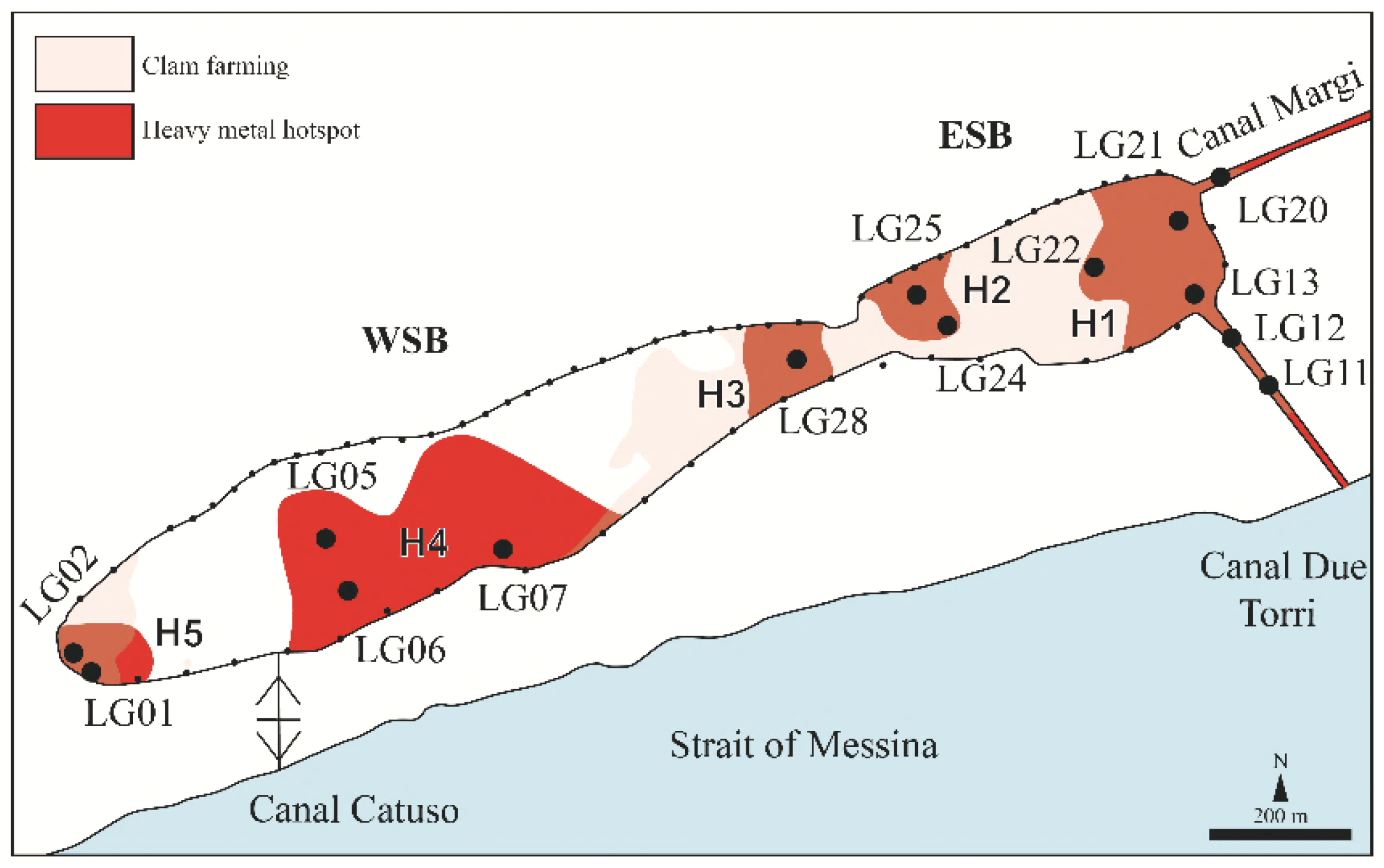
Different grade and typologies of human impact may be expected in LG. In this respect, the contextual investigation on chemical elements [15] provided useful basic information. A synthetic map, here elaborated from their data (Figure 17), showed the areal distribution of five main chemical hotspots related, in the complex, to the heavy metals Zn, Pb, Tl, Ni, Cu, Cr, Cd. The easternmost hotspot (H1 in Figure 17), including the areas of Canal Margi and Canal Due Torri, was located in the eastern edge of the ESB; this hotspot was the most consistent, being present Zn (in front of Canal Margi), Tl (in front of Canal Margi), Pb (in front of both canals Margi and Due Torri; maximum value: LG21), and Cd (in front of Due Torri canal; maximum value: LG13). Two minor hotspots (H2 and H3 in Figure 17) were evidenced in the neck zone; H2 and H3 showed the occurrence of all the heavy metals studied, being present Zn, Pb, Cu (maximum value: LG25), Cr, Cd. The H4 western hotspot, located in the centre of the WSB, was the most extended and related to the Zn (maximum value: LG07), Tl, and Cr (maximum value: LG07). The westernmost hotspot (H5 in Figure 17) was in the edge of the WSB; the hotspot was related to Pb, Tl (maximum value: LG02), and Cr.
By comparing the main heavy metal hotspots (H1–5) reported in Figure 17 with the QGIS distribution maps of the mean, sorting, kurtosis, and skewness (Figure 7a–d,12), as well as with the morpho-bathymetric data (Figure 3b), it was evident as no significative correlations were found. Differently, a significative matching between the main heavy metal hotspots (Figure 17) and the hotspots of some metals (Al, Fe, and Mg) [15] was evidenced. A match was also identified between chemical and malacofauna (Figure 14) hotspots, but further research should be required for a better explanation of this evidence.
It must be underlined that the metal concentration ranges [15] were all compatible with pre-industrial background values. Moreover, the concentrations normalized to geogenic metals, being very low, would suggest prevalent natural origins for the heavy metals. Their presence in the bioavailable fraction should be geogenic and due to the release of metals from the source rocks. Chemical-physical weathering due to rainwaters infiltrating in the bedrock (actual alluvial deposits, middle Pleistocene sediments, and high-grade metamorphic rocks - Aspromonte Unit), outcropping in the upstream surrounding areas, could be responsible for delivering metals that could deposit in the lake bottom bed. Low concentrations of heavy metals in LG waters, found in the past [43], would better agree with mostly natural origins for these metals. Very low concentrations of metals recently found in edible filtering feeder clams of LG [14] further would support this hypothesis.
7. Conclusions
The detailed and updated morpho-bathymetric map of the lake bottom together with the first georeferenced maps of the main sedimentological statistical parameters (mean, sorting, kurtosis, skewness) of the bottom bed provided a solid background to better understand the geological, sedimentological, and ecological processes affecting LG.
The mixed composition of the bottom clastic sediments, due to quartzo-lithic sands and consistent amounts of calcareous bioclasts (connected with the clam farming), was evidenced for the first time in the sediments of the Peloritani coastal lagoons. The heterogeneous textures of the bottom shallowest sediments were indicative of low degree of confinement and high-energy environment. These conditions, established after the re-connection of the lagoon waters with the sea in the 18th century, were analogous to those characterising the early Bronze Age.
Lastly, considering the absence of evident correlations among the areal distribution of the textural parameters and the heavy metal hotspots and the evident correlation between the heavy metal hotspots and some metals (Al, Fe, Mg), a geogenic origin for the heavy metals may be presumed and significant anthropogenic contaminations may be excluded.
On the base of the above, the present research highlighted as the proposed multi-disciplinary approach, based on compared QGIS maps and multivariate statistics, could provide a useful tool for assessing the natural or anthropogenic source of contaminants in sediments of vulnerable coastal lakes, allowing a better evaluation of the ecological risk.
Supplementary Materials
The following supporting information can be downloaded at the website of this paper posted on Preprints.org. Table S1: Main statistical data (In SD: Inclusive Standard Deviation, In K: Kurtosis, In Sk: Skewness, Mean, and texture) of the total sediment samples.; Table S2: Main statistical data (In SD: Inclusive Standard Deviation or Sorting, In K: Kurtosis, In Sk: Skewness, Mean, and texture) of the silty to clayish fraction of the total sediment samples.
Author Contributions
Conceptualization, RS, SG; methodology, RS, SG; software, MGY, MA, RKM, SZ; validation, RS, SG; formal analysis, RS, MGY, ACM, RKM, SG; investigation, RS, MGY, ACM, RKM; data curation, MGY, MA, RKM; writing—original draft preparation; RS, SG; writing—review & editing, RS, SG; visualization, RS, MGY, ACM, MA, RKM, SZ, SG; supervision, RS, SG. All authors have read and agreed to the published version of the manuscript.
Funding
This research received no external funding.
Acknowledgments
The authors are grateful to the Editor and the three reviewers who strongly improved the present paper.
Conflicts of Interest
The authors declare no conflicts of interest.
References
- Maccarrone, V.; Scandura, P.; La Rosa, S.D. The Integrated Coastal Zone Management in the Anthropocene. In Coastal Sustainability Insights from Southeast Asia and Beyond; Maccarrone, V., Akhir Fadzil, M., Eds.; Springer Nature: Cham, Switzerland, 2024; Volume 39, pp. 1–20. [Google Scholar] [CrossRef]
- Young, A. F. Coastal megacities, environmental hazards and global environmental change. In Megacities and the Coast: Risk, resilience and Transformation; Pelling, M., Blackburn, S., Eds.; Earthscan from Routledge: London, UK, 2014; Volume 3, pp. 70–99. [Google Scholar] [CrossRef]
- Dias, G. M.; Edwards, G. C. Differentiating natural and anthropogenic sources of metals to the environment. Hum. Ecol. Risk Assess. 2003, 9, 699–721. [Google Scholar] [CrossRef]
- Masindi, V.; Mkhonza, P.; Tekere, M. Sources of heavy metals pollution. In Remediation of heavy metals; Springer Nature: Cham, Switzerland, 2021; pp. 419–454. [Google Scholar] [CrossRef]
- Kostka, A.; Leśniak, A. Natural and anthropogenic origin of metals in lacustrine sediments; assessment and consequences—A case study of Wigry lake (Poland). Minerals 2021, 11, 158. [Google Scholar] [CrossRef]
- Umgiesser, G.; Ferrarin, C.; Cucco, A.; De Pascalis, F.; Bellafiore, D.; Ghezzo, M.; Bajo, M. Comparative hydrodynamics of 10 Mediterranean lagoons by means of numerical modeling. J. Geophys. Res. Oceans 2014, 119, 2212–2226. [Google Scholar] [CrossRef]
- Gooch, G. D. Coastal Lagoons in Europe: Integrated Water Resource Strategies; Lillebø, A.I., Stalnacke, P., Gooch, G.D., Eds.; IWA Publishing: London, UK, 2015; pp. 1–256. [Google Scholar]
- Longhitano, S. G.; Della Luna, R.; Milone, A. L.; Cilumbriello, A.; Caffau, M.; Spilotro, G. The 20,000-years-long sedimentary record of the Lesina coastal system (southern Italy): from alluvial, to tidal, to wave process regime change. The Holocene 2016, 26, 678–698. [Google Scholar] [CrossRef]
- Morales-Marin, L. A.; Carr, M.; Sadeghian, A.; Lindenschmidt, K. E. Climate change effects on the thermal stratification of Lake Diefenbaker, a large multi-purpose reservoir. CWRJ 2021, 46(1-2), 1–16. [Google Scholar] [CrossRef]
- Regione Siciliana. Riserva Naturale Laguna di Capo Peloro. Available online: https://orbs.regione.sicilia.it/aree-protette/riserve-naturali-siciliane/164-riserva-naturale-orientata-laguna-capo-peloro.html (accessed on 2 July 2025).
- Somma, R.; Spoto, S. E.; Giacobbe, S. Geological and structural framework, inventory, and quantitative assessment of geodiversity: the case study of the lake Faro and lake Ganzirri global geosites (Italy). Geosciences 2024, 14, 236. [Google Scholar] [CrossRef]
- Somma, R.; Giuffrè, E.; Amonullozoda, S.; Spoto, S. E.; Giacobbe, A.; Giacobbe, S. Geological and Ecological Insights on the Lake Faro Global Geosite Within the Messina Strait Framework (Italy). Geosciences 2024, 14, 319. [Google Scholar] [CrossRef]
- Di Bella, G.; Litrenta, F.; Potortì, A. G.; Giacobbe, S.; Nava, V.; Puntorieri, D.; Lo Turco, V. Plasticizers and Bisphenols in Sicilian Lagoon Bivalves, Water, and Sediments: Environmental Risk in Areas with Different Anthropogenic Pressure. Environments 2025, 12, 305. [Google Scholar] [CrossRef]
- Giacobbe, S.; Nava, V.; Sgrò, B.; Scarpa, F.; Sanna, D.; Casu, M.; Di Bella, G. Mineral content in clam species from Sicily and Sardinia: A geographical, temporal and species-specific statistical comparison. Chemosphere 2025, 377, 144328. [Google Scholar] [CrossRef] [PubMed]
- Cigala, R.M.; Crea, F.; Somma, R.; De Stefano, C.; Ghanadzadeh Yazdi, M.; Giacobbe, S. Determination of potential contaminants in sediments from Lake Ganzirri brackish pond (Capo Peloro lagoon, Italy) by different instrumental techniques. Chemosphere CHEM147424.
- Miall, A. D. Principles of sedimentary basin analysis, 3rd Edition; Miall, A. D., Ed.; Springer Berlin: Heidelberg, 2000; pp. 1–616. [Google Scholar] [CrossRef]
- Nichols, G. Sedimentology and Stratigraphy, 2nd Edition ed; Wiley-Blackwell, John Wiley & Sons: Hoboken, New Jersey, USA, 2009; pp. 1–432. [Google Scholar]
- Reading, H. G. Sedimentary environments: processes, facies and stratigraphy; Reading, H. G., Ed.; John Wiley & Sons: Hoboken, New Jersey, USA, 2009; pp. 1–688. [Google Scholar]
- Allen, J. R. Principles of physical sedimentology; Allen, J. R., Ed.; Springer Science & Business Media, Blackburn Press: Caldwell, New Jersey, USA, 2012; pp. 1–272. [Google Scholar]
- Boggs, S. Principles of sedimentology and stratigraphy, 5th edition; Boggs, S., Ed.; Pearson Education Limited, Harlow, Essex, England and Associated Companies throughout the world, 2014; pp. 1–676. [Google Scholar]
- Hjulstrom, F. Studies of Morphological Activity of Rivers as Illustrated by the River Fyris. Bull. Geol. Inst. Univ. Uppsala 1935, 25, 221–527. [Google Scholar]
- Bonardi, G.; Giunta, G.; Liguori, V.; Perrone, V.; Russo, M.; Zuppetta, A. Schema geologico dei Monti Peloritani. Boll. Soc. Geol. It. 1976, 95, 49–74. [Google Scholar]
- Cirrincione, R.; Fazio, E.; Fiannacca, P.; Ortolano, G.; Pezzino, A.; Punturo, R. The Calabria-Peloritani Orogen, a composite terrane in Central Mediterranean; Its overall architecture and geodynamic significance for a pre-Alpine scenario around the Tethyan basin. Period. Mineral. 2015, 84, 701–749. [Google Scholar] [CrossRef]
- Catalano, S.; Cirrincione, R.; Mazzoleni, P.; Pavano, F.; Pezzino, A.; Romagnoli, G.; Tortorici, G. The effects of a Meso-Alpine collision event on the tectono-metamorphic evolution of the Peloritani mountain belt (eastern Sicily, southern Italy). Geol. Mag. 2018, 155, 422–437. [Google Scholar] [CrossRef]
- Somma, R. The Inventory and Quantitative Assessment of Geodiversity as Strategic Tools for Promoting Sustainable Geoconservation and Geo-Education in the Peloritani Mountains (Italy). Educ. Sci. 2022, 12, 580. [Google Scholar] [CrossRef]
- Lentini, F.; Catalano, S.; Carbone, S. Note Illustrative della Carta Geologica della Provincia di Messina Scala 1: 50.000 2000, 1–70.
- Segre, A.G.; Bagnala, R.; Sylos Labini, S. Holocene evolution of the Pelorus headland, Sicily. Quat. Nova 2004, 8, 69–78. [Google Scholar]
- Perri, F.; Dominici, R.; Le Pera, E.; Chiocci, F.L.; Martorelli, E. Holocene sediments of the Messina Strait (southern Italy): Relationships between source area and depositional basin. Mar. Pet. Geol. 2016, 77, 553–566. [Google Scholar] [CrossRef]
- Somma, R. Petrographic and Textural Characterization of Beach Sands Contaminated by Asbestos Cement Materials (Cape Peloro, Messina, Italy): Hazardous Human-Environmental Relationships. Geosciences 2024, 14, 167. [Google Scholar] [CrossRef]
- Bottari, A.; Bottari, C.; Carveni, P.; Giacobbe, S.; Spanò, N. Genesis and geomorphologic and ecological evolution of the Ganzirri salt marsh (Messina, Italy). Quat. Int. 2005, 140141(VII(1), 150–158. [Google Scholar] [CrossRef]
- Guarnieri, P.; Pirrotta, C. The response of drainage basins to the late Quaternary tectonics in the Sicilian side of the Messina Strait (NE Sicily). Geomorphology 2008, 95, 260–273. [Google Scholar] [CrossRef]
- Doglioni, C.; Ligi, M.; Scrocca, D.; Bigi, S.; Bortoluzzi, G.; Carminati, E.; Cuffaro, M.; D’Oriano, F.; Forleo, V.; Muccini, F. The tectonic puzzle of the Messina area (southern Italy): Insights from new seismic reflection data. Sci. Rep. 2012, 2, 970. [Google Scholar] [CrossRef]
- Bottari, C.; Carveni, P. Archaeological and historiographical implications of recent uplift of the Peloro Peninsula, NE Sicily. Quat. Res. 2009, 72, 38–46. [Google Scholar] [CrossRef]
- Palli, J.; Monaco, L.; Bini, M.; Cosma, E.; Giaccio, B.; Izdebski, A.; Masi, A.; Mensing, S.; Piovesan, G.; Rossi, V.; Sadori, L.; Wagner, B.; Zanchetta, G. The recent evolution of the salt marsh ‘Pantano Grande’(NE Sicily, Italy): interplay between natural and human activity over the last 3700 years. J. Quat. Sci. 2024, 39, 327–339. [Google Scholar] [CrossRef]
- Palli, J.; Fiolna, S.; Bini, M.; Cappella, F.; Izdebski, A.; Masi, A.; Zanchetta, G. The human-driven ecological success of olive trees over the last 3700 years in the Central Mediterranean. Quat. Sci. Rev. 2025, 356, 109313. [Google Scholar] [CrossRef]
- Manganaro, A.; Pulicanò, A.; Sanfilippo, G. M. Temporal evolution of the area of Capo Peloro (Sicily, Italy) from pristine site into urbanized area. Transit. Waters Bull. 2011, 5, 23–31. [Google Scholar] [CrossRef]
- Leonardi, M.; Azzaro, F.; Azzaro, M.; Caruso, G.; Mancuso, M.; Monticelli, L. S.; Zaccone, R. A multidisciplinary study of the Cape Peloro brackish area (Messina, Italy): characterisation of trophic conditions, microbial abundances and activities. Mar. Ecol. 2009, 30, 33–42. [Google Scholar] [CrossRef]
- Caruso, G.; Leonardi, M.; Monticelli, L. S.; Decembrini, F.; Azzaro, F.; Crisafi, E.; Vizzini, S. Assessment of the ecological status of transitional waters in Sicily (Italy): First characterisation and classification according to a multiparametric approach. Mar. Pollut. Bull. 2010, 60, 1682–1690. [Google Scholar] [CrossRef]
- Sanfilippo, M.; Albano, M.; Manganaro, A.; Capillo, G.; Spanò, N.; Savoca, S. Spatiotemporal organic carbon distribution in the Capo Peloro Lagoon (Sicily, Italy) in relation to environmentally sustainable approaches. Water 2022, 14, 108. [Google Scholar] [CrossRef]
- Ferrarin, C.; Bergamasco, A.; Umgiesser, G.; Cucco, A. Hydrodynamics and spatial zonation of the Capo Peloro coastal system (Sicily) through 3-D numerical modeling. ESCO 2014, 37, 79–93. [Google Scholar] [CrossRef]
- Gianguzza, A.; Mannino, M. R.; Olivo, A.; Orecchio, S. Occurrence and concentration of PAHS in clams and sediments of the marine coastal lagoon of Ganzirri (Italy). Extraction, GC-MS analysis, distribution and sources. Fresenius Environ. Bull. 2006, 15(9a), 1026–1033. [Google Scholar]
- Caristi, C.; Cimino, G.; Ziino, M. Inquinamento da metalli pesanti – Nota VI Indagine sul grado di contaminazione delle acque e dei sedimenti dei laghi di Faro e di Ganzirri (Messina). Atti Soc. Pelorit. Sc. Fis. Mat. Nat. 1980, XXVI, 203–214. [Google Scholar]
- Lo Coco, F.; Lanuzza, F.; Adami, G.; Cappellano, G.; Cozzi, F.; Mondello, F. La qualità delle acque dei laghi di Faro e di Ganzirri (Messina) adibiti a miticoltura. Dosaggio di metalli pesanti. Proceedings of La qualità dei prodotti per la competitività delle imprese e la tutela dei consumatori, XXII Congresso Nazionale di Merceologia, Università Roma Tre, Roma (Italy), 2–4 March 2006. [Google Scholar]
- Abbruzzese, D.; Genovese, S. Osservazioni geomorfologiche e fisico-chimiche sui laghi di Ganzirri e di Faro. Boll. Pesca Piscic. Idrobiol. 1952, 7, 1–20. [Google Scholar]
- Friedman, G. M. Distinction between dune, beach, and river sands from their textural characteristics. J. Sediment. Res. 1961, 31, 514–529. [Google Scholar] [CrossRef]
- Folk, R.L.; Ward, W.C. Brazos River bar: a study of significance of grain size parameters. J. Sediment. Petrol. 1957, 27, 3–26. [Google Scholar] [CrossRef]
- Blott, S.J.; Croft, D.J.; Pye, K.; Saye, S.E.; Wilson, H.E. Particle size analysis by laser diffraction. Geol. Soc. Spec. Publ. 2004, 232, 63–73. [Google Scholar] [CrossRef]
- Eshel, G.; Levy, G.J.; Mingelgrin, U.; Singer, M.J. Critical Evaluation of the Use of Laser Diffraction for Particle-Size Distribution Analysis. Soil Sci. Soc. Am. J. 2004, 68, 736–743. [Google Scholar] [CrossRef]
- Fedra, K.; Feoli, E. GIS technology and spatial analysis in coastal zone management. EEZ Technology 1998, 3, 1–25. [Google Scholar]
- Clarke, K.R.; Warwick, R.M. Change in Marine Communities: An Approach to Statistical Analysis and Interpretation, 2nd ed.; PRIMER-E, Ltd., Plymouth Marine Laboratory: Plymouth, 2001. [Google Scholar]
- Sarconi, M. Istoria de’ fenomeni del tremuoto avvenuto nelle Calabrie e nel Valdemone nell’anno 1783, posta in luce dalla Reale Accademia delle Scienze e delle Belle Lettere di Napoli; Campo, G., Ed.; Reale Accademia delle Scienze e delle Belle Lettere di Napoli: Napoli, Italy, 1784; pp. 1–197. [Google Scholar]
- Vivenzio, G. Historia dei tremuoti avvenuti nella provincia di Calabria ulteriore e nella città di Messina nell’anno 1783 e di quanto nelle Calabrie fu fatto per il suo risorgimento fino al 1787, preceduta da una Teoria, ed Istoria Generale de’ Tremuoti. In Stamperia Regale, Napoli, Italy; 1788; Volume 2, pp. 1–441. [Google Scholar]
- Maramai, A.; Graziani, L.; Brizuela Reyes, B. Italian Tsunami Effects Database (ITED) (Version 1.0) [Data set]; Istituto Nazionale di Geofisica e Vulcanologia (INGV), 2019. [Google Scholar] [CrossRef]
- Guelorget, O.; Perthuisot, J. P. Le domaine paralique. Expressions géologiques, biologiques et économiques du confinement. In Trav. Lab. Géol.; Ec. Norm. Super.: Paris (France), 1983; Volume 16, pp. 1–136. [Google Scholar]
Figure 1.
(a) Sketch geological map of the NE end of the Peloritani Mountains (Messina, Italy). In the rectangle the localization of the NE edge of Messina. (b) Legend of the lithological map. (c) Localization of the study area. (d) Geological and structural map of the Cape Peloro peninsula. The black line inside Lake Faro (me) represents the morphological escarpment along the platform edge on the westmost side of the lake. Acronyms – GL: Ganzirri Lake, FL: Faro Lake. 1: Canal Catuso (actually closed), 2: Canal Due Torri, 3: Canal Margi, 4: Canal degli Inglesi, 5: Canal Faro.
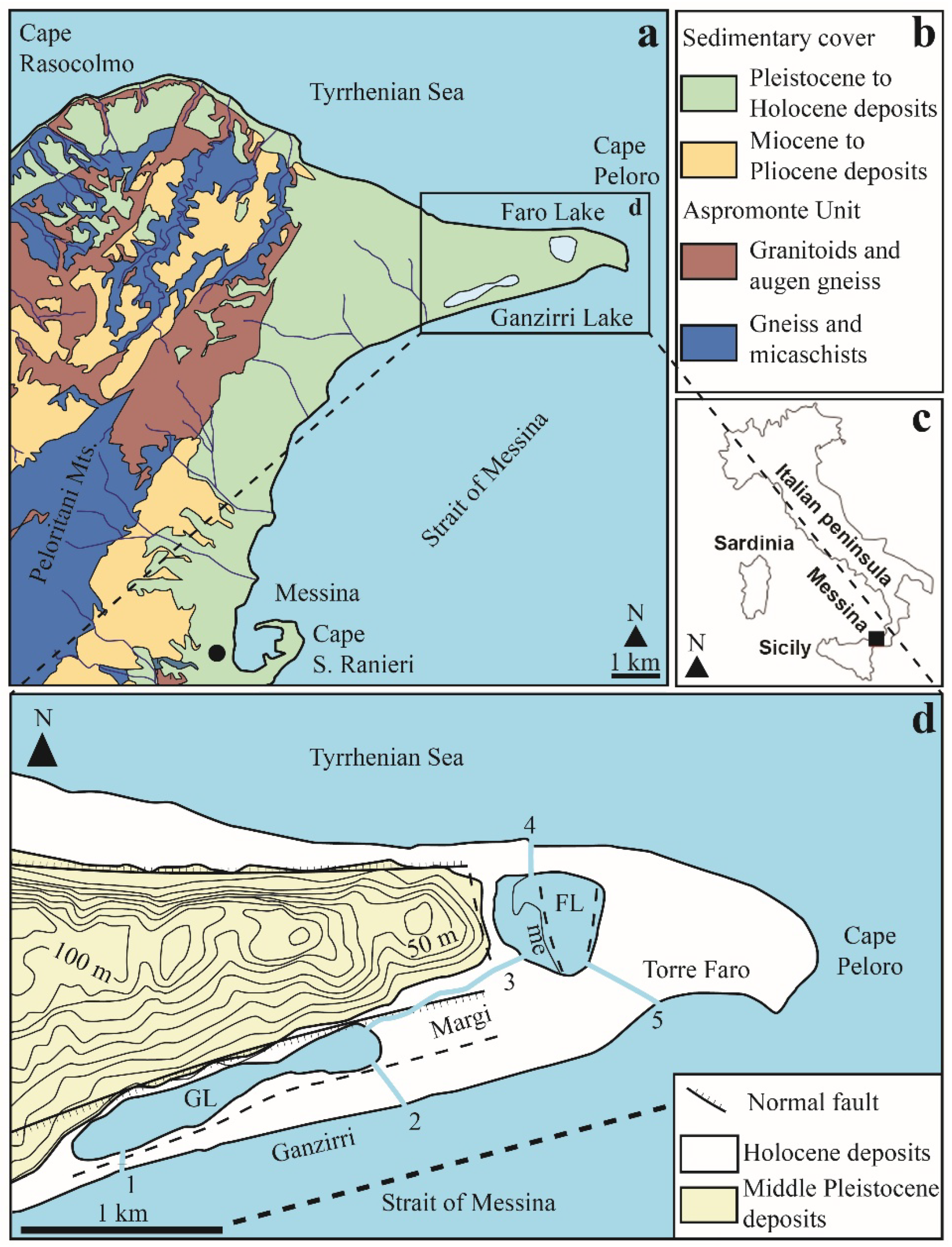
Figure 2.
Stratigraphic record of the Lake Ganzirri sediments (modified after [34]).
Figure 2.
Stratigraphic record of the Lake Ganzirri sediments (modified after [34]).
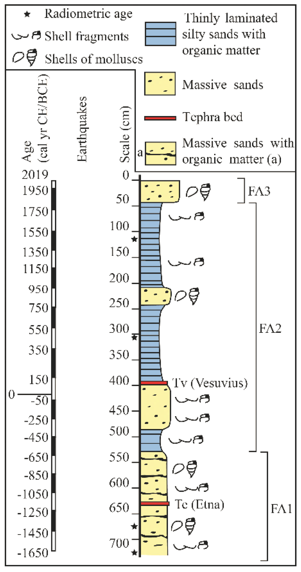
Figure 3.
QGIS maps of Lake Ganzirri. Acronyms. ESB: eastern sub-basin. WSB: western sub-basin. (a) Localization of the sixty-eight (68) georeferenced stations used for reconstructing the lake bathymetry. Symbols. Red circle: bottom sediment. Yellow circle: unknown bedrock. Light blue square: drilling site [34]. (b) Bathymetric contour map of the lake bottom. The gradient color scale (on the left) indicates areas with depths variable from shallower (red) to deeper (blue) values. Isobaths (-m) are spaced at 0.5 m.
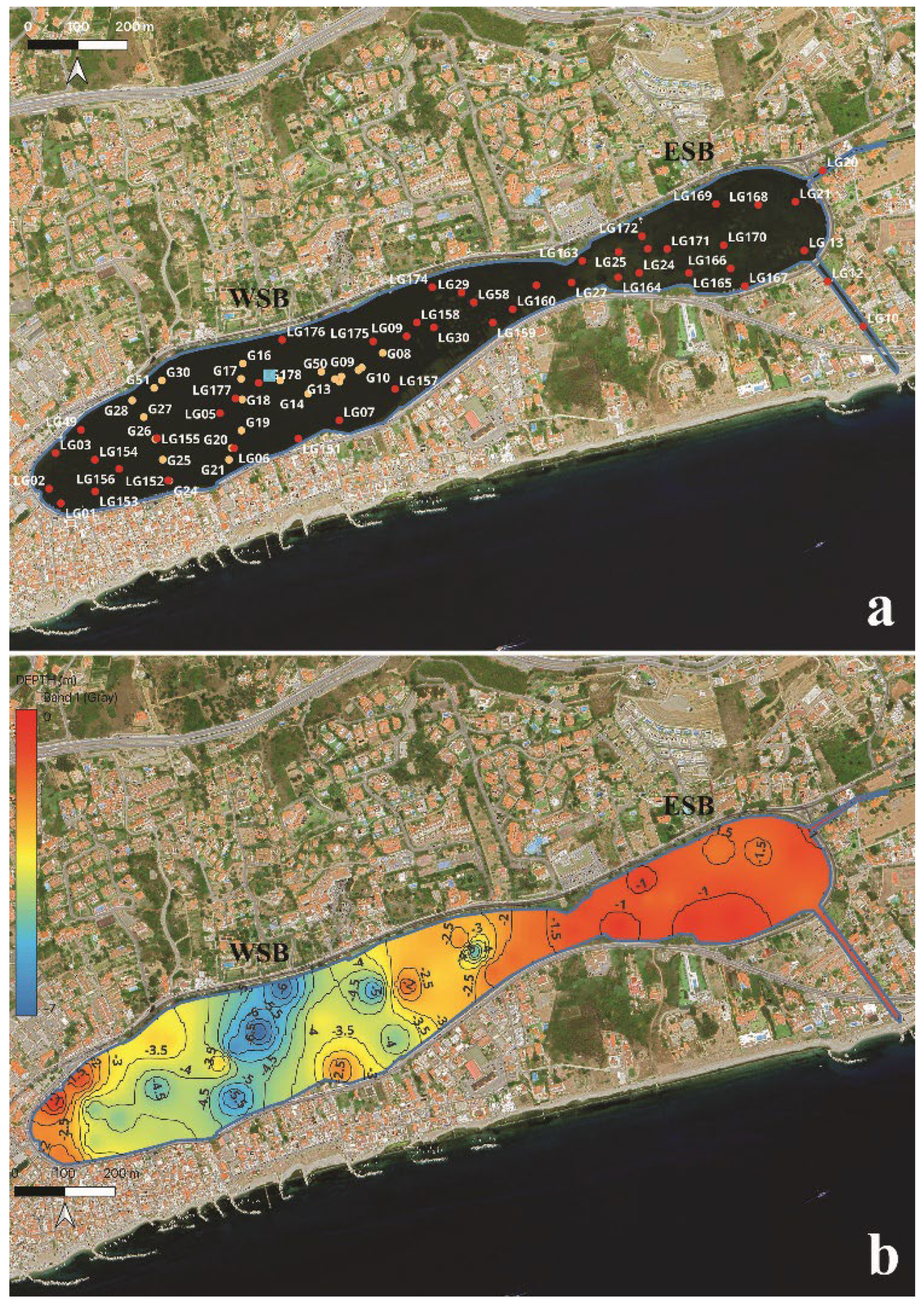
Figure 4.
ENE-WSW trending simplified structural cross section of the Lake Ganzirri showing a presumed fault system affecting the middle Pleistocene Sands and Gravels of the Messina Formation (sealed by overlying upper Holocene sediments). The unconformity among these two successions was not reported. The Holocene beachrock is reported with the gray line (dotted line where it is presumed). The altitude was exaggerated with respect to the lake length, because of the very low depth/length ratio (see different horizontal and vertical graphic scales).
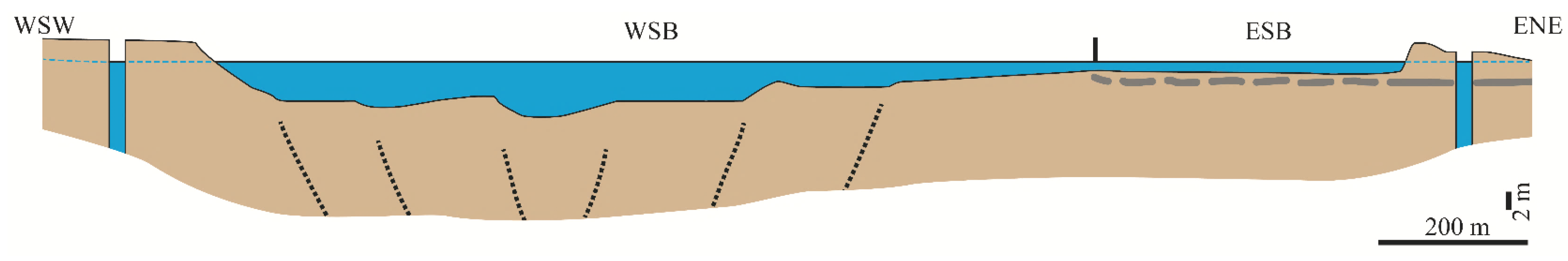
Figure 5.
Sediments of Lake Ganzirri. (a) Cumulative retained oversize curves related to the grain size distribution of the total sediment samples (solid black lines) and on the neighboring beaches (red dotted line). The granulometric zone of the Lake Ganzirri deposits is outlined with the light blue dotted line. (b) Ternary diagram (Gravel, Sand, Mud) showing the composition of the total sediment samples.
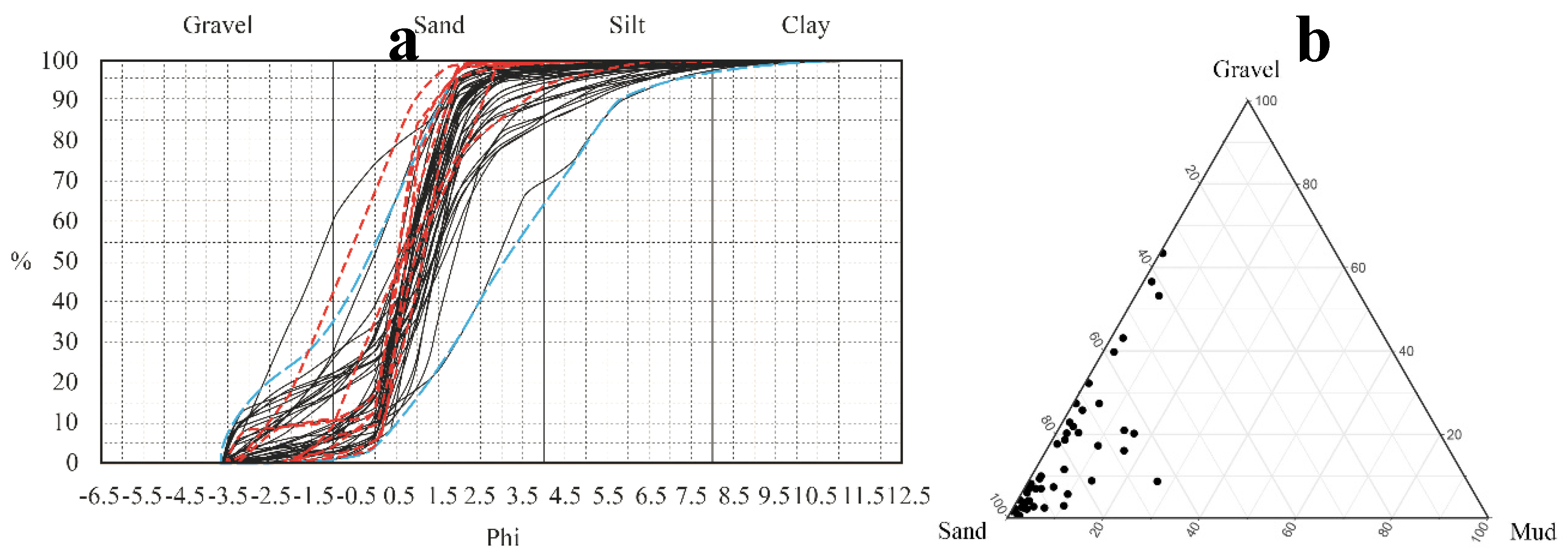
Figure 6.
Main textural statistical data of the total sediment samples: (a) Mean. (b) Sorting. (c) Kurtosis. (d) Skewness. Data set based on 46 samples.
Figure 6.
Main textural statistical data of the total sediment samples: (a) Mean. (b) Sorting. (c) Kurtosis. (d) Skewness. Data set based on 46 samples.
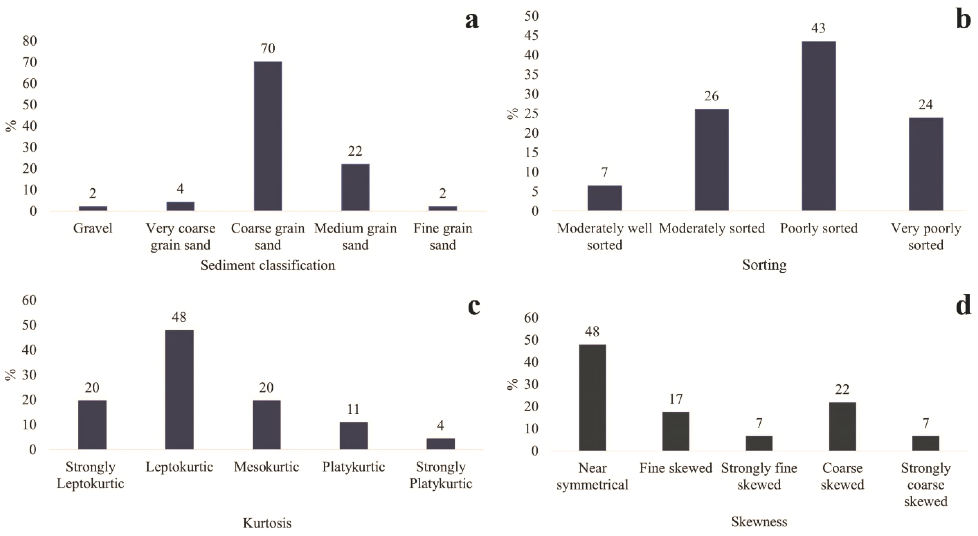
Figure 7.
QGIS maps of the main textural statistical data related to grain size analyses of the coarse-to fine-grained sediments. (a) Mean. (b) Sorting. (c) Kurtosis. (d) Skewness.
Figure 7.
QGIS maps of the main textural statistical data related to grain size analyses of the coarse-to fine-grained sediments. (a) Mean. (b) Sorting. (c) Kurtosis. (d) Skewness.
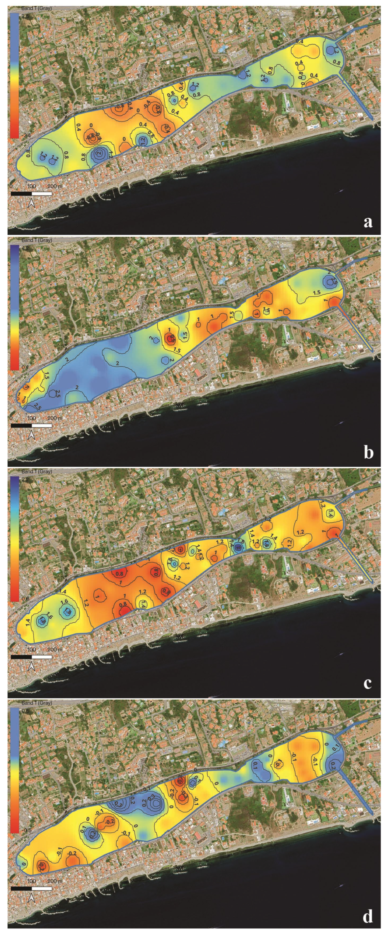
Figure 8.
(a) Scatter plot of mean vs skewness for shallow bottom sands of the LG. (b) Scatter plot of mean vs sorting for shallow bottom sands of the LG. The Peloro peninsula beach samples were also reported for comparative purposes. The diagram was elaborated by using excel software. Symbols: LG samples (solid green circles). Peloro peninsula beach samples (solid red circles).
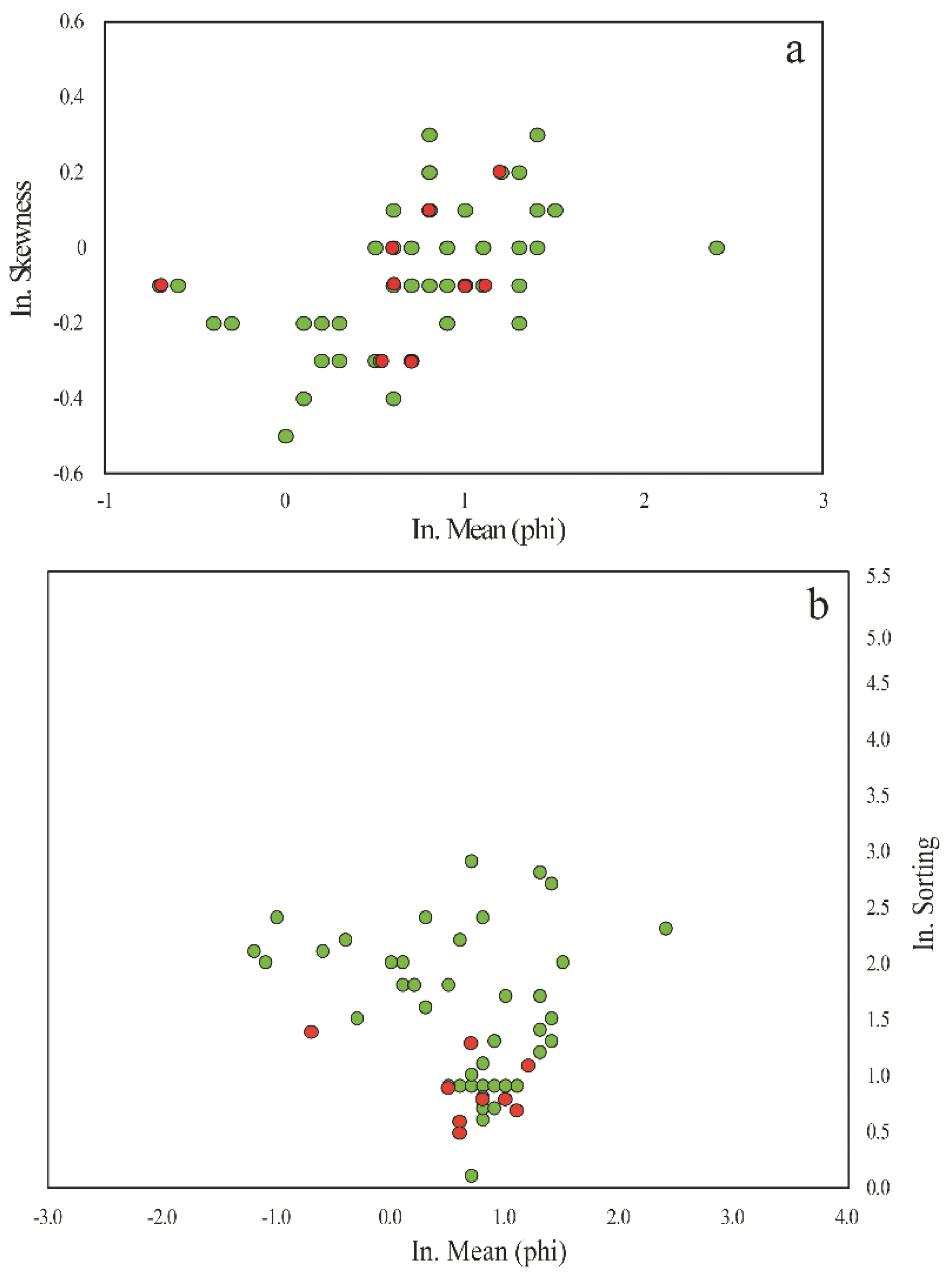
Figure 9.
Cluster analysis carried out on the sediment samples. Depth as discriminant factor is put in evidence (see top right). The four groups recognized by slicing at 2.5 Euclidean distance are indicated, except for the single sample LG06 (analysis and graph elaborated by using the PRIMER 6 statistical package [50]).
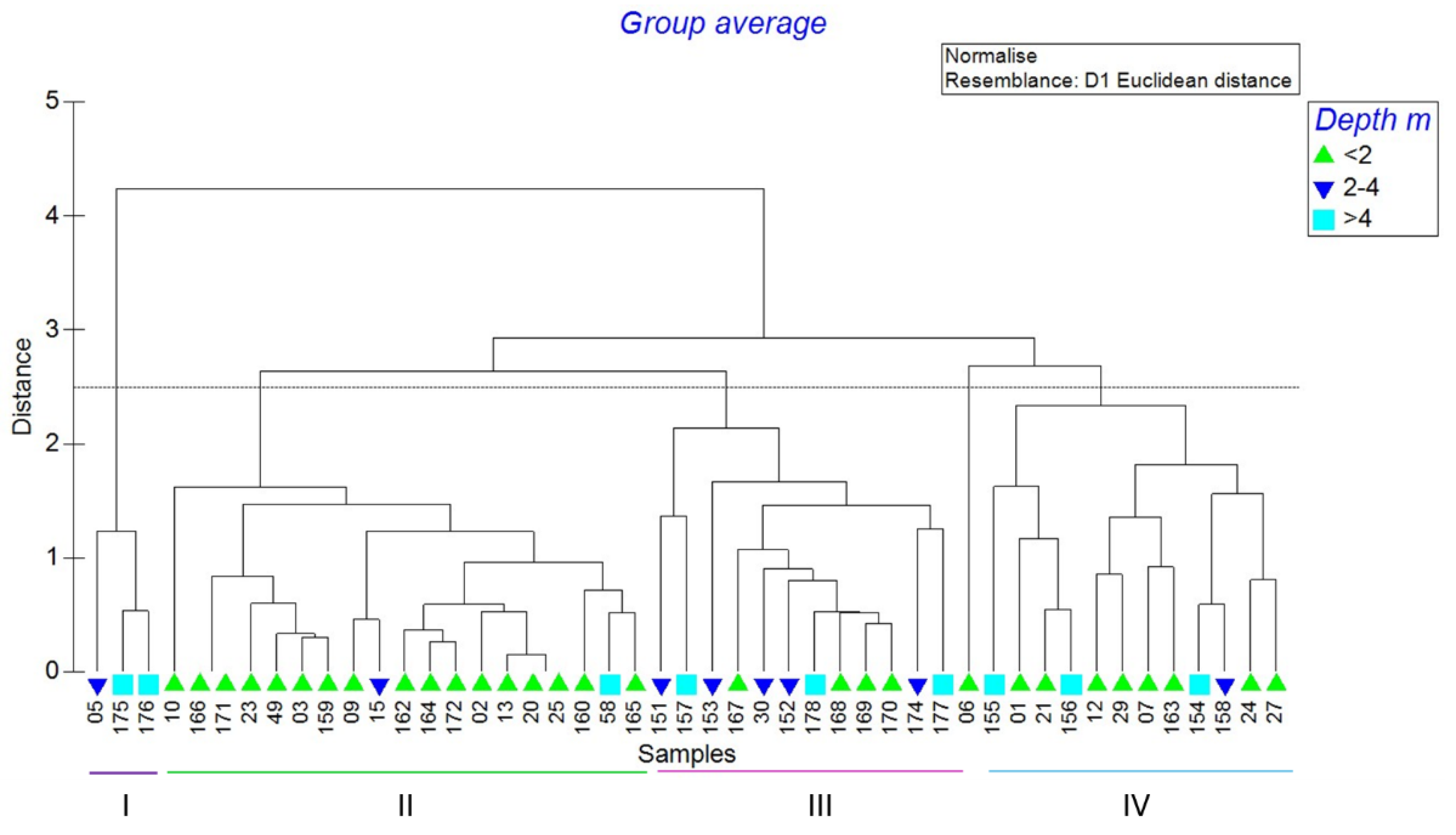
Figure 10.
(a) Frequency and (b) cumulative curves related to the silty to clayish fraction of the total sediment samples collected on the LG bottom. The graphs were obtained using the workstation associated with the Mastersizer laser diffractometer.
Figure 10.
(a) Frequency and (b) cumulative curves related to the silty to clayish fraction of the total sediment samples collected on the LG bottom. The graphs were obtained using the workstation associated with the Mastersizer laser diffractometer.
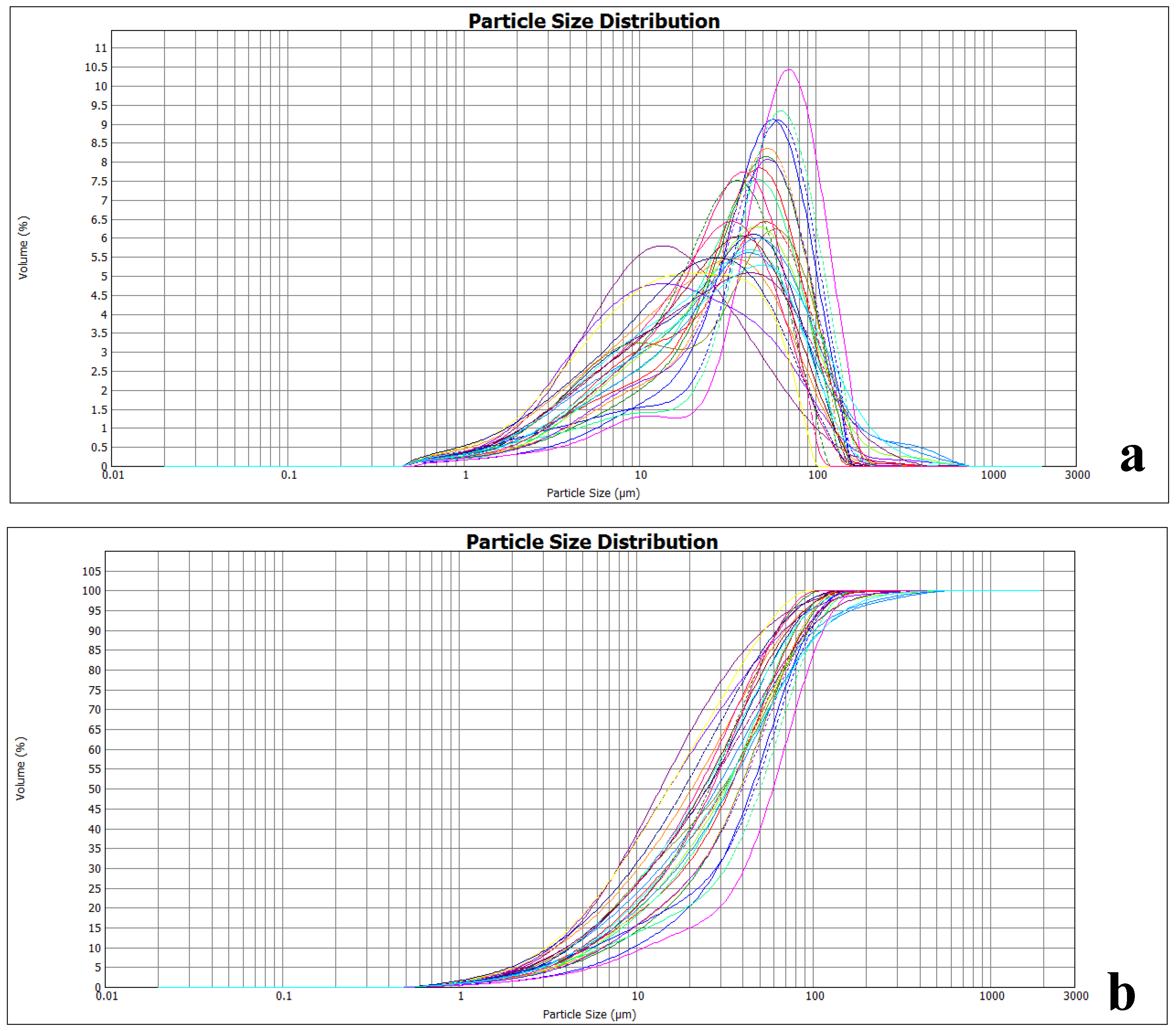
Figure 11.
Main statistical data of the silty to clayish fraction of the total bottom sediments: (a) Mean. (b) Kurtosis. (c) Skewness. Data set based on 46 samples. The frequency % of each category for all considered parameters is represented.
Figure 11.
Main statistical data of the silty to clayish fraction of the total bottom sediments: (a) Mean. (b) Kurtosis. (c) Skewness. Data set based on 46 samples. The frequency % of each category for all considered parameters is represented.
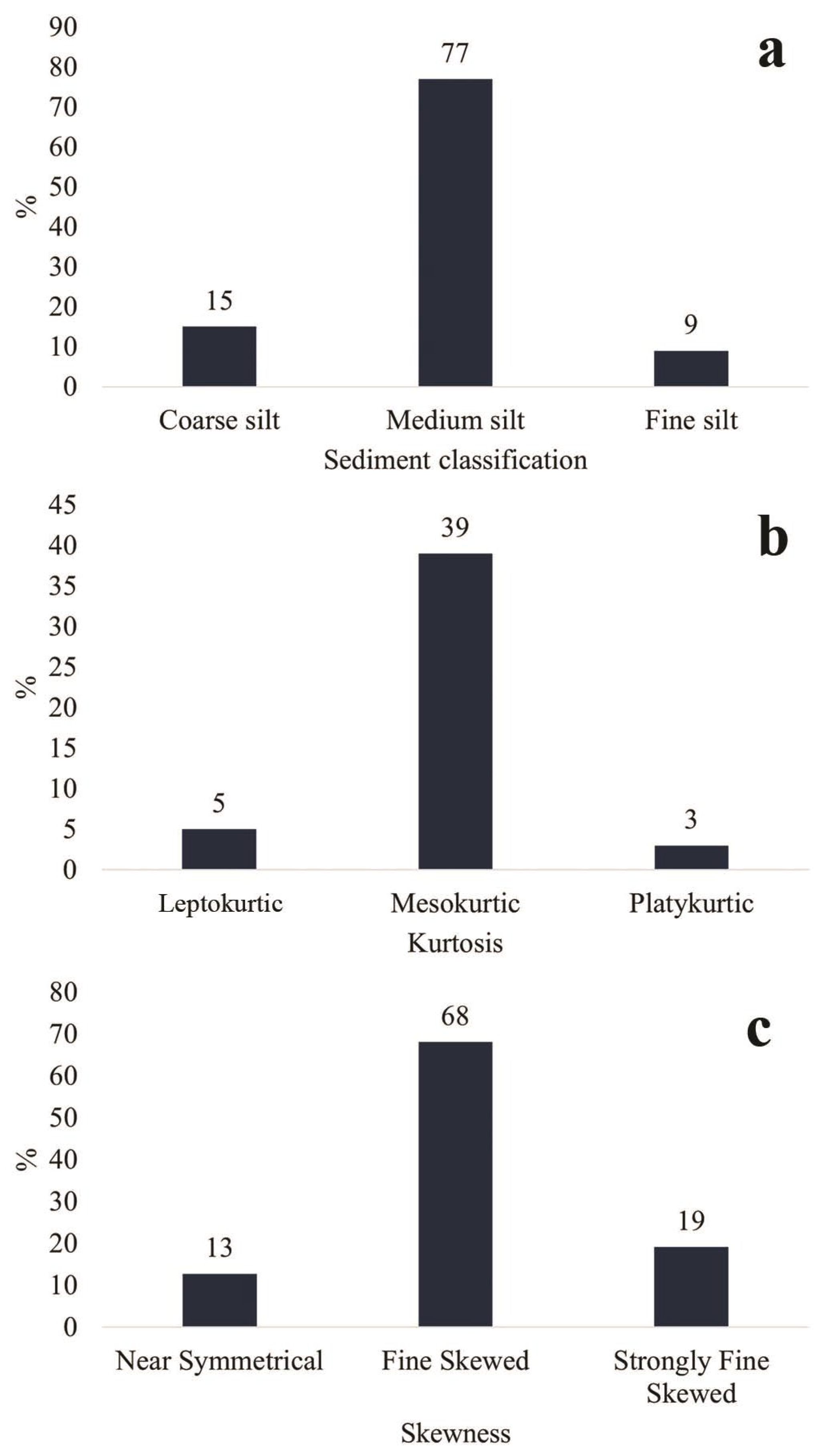
Figure 12.
QGIS maps of the main textural statistical data related to grain size analyses of the fine fractions of the bottom sediments. (a) Mean. (b) Sorting. (c) Kurtosis. (d) Skewness.
Figure 12.
QGIS maps of the main textural statistical data related to grain size analyses of the fine fractions of the bottom sediments. (a) Mean. (b) Sorting. (c) Kurtosis. (d) Skewness.
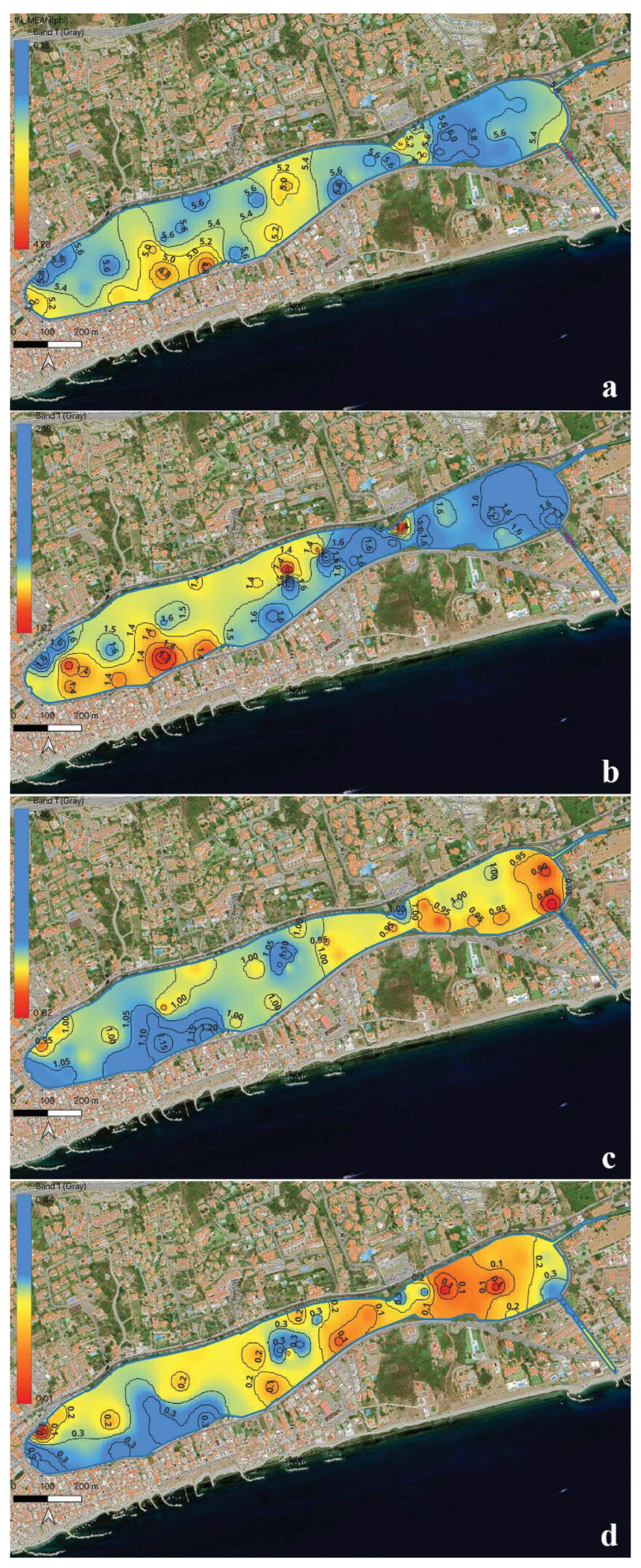
Figure 13.
Thin section of sands aggregated in epoxy resin, observed under petrographic microscopy with transmitted light (Sample LG13) (a–i: parallel polars; a’–i’: crossed polars). (a–a’) Subrounded and subangular grains of quartz. Skeletal remains of a spirorbid polychaete are present on the right part of the photo. (b–b’) Angular grains of quartz. Subrounded grain of gneiss is observable on the bottom left. (c–c’) Subrounded and subangular grains of quartz. Subrounded grain of gneiss is observable on the bottom right. (d–d’) Subangular grains of quartz. Subrounded grain of gneiss is observable on the middle left. (e–e’) Subrounded grain of gneiss showing schistosity. (f–f’) Subangular grains of gneiss. (g–g’) Well rounded grain of feldspar (microcline) (h–h’) Subrounded grains of gneiss. (i–i’) Subrounded grain of gneiss.
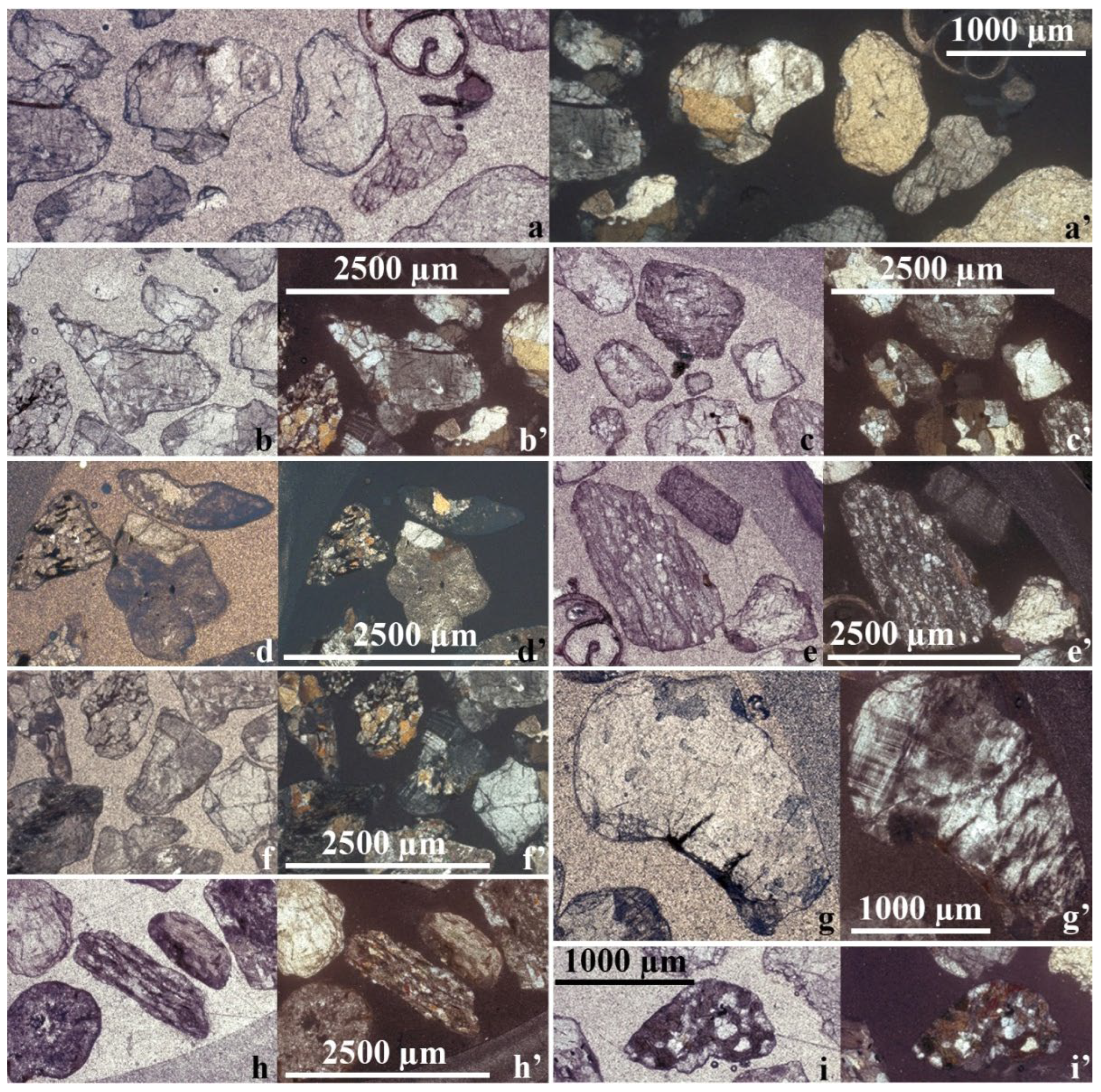
Figure 14.
QGIS map of the distribution related to the coarse bioclasts (size > 1 mm) present in the bottom sediments. The concentrations are expressed as g%.
Figure 14.
QGIS map of the distribution related to the coarse bioclasts (size > 1 mm) present in the bottom sediments. The concentrations are expressed as g%.
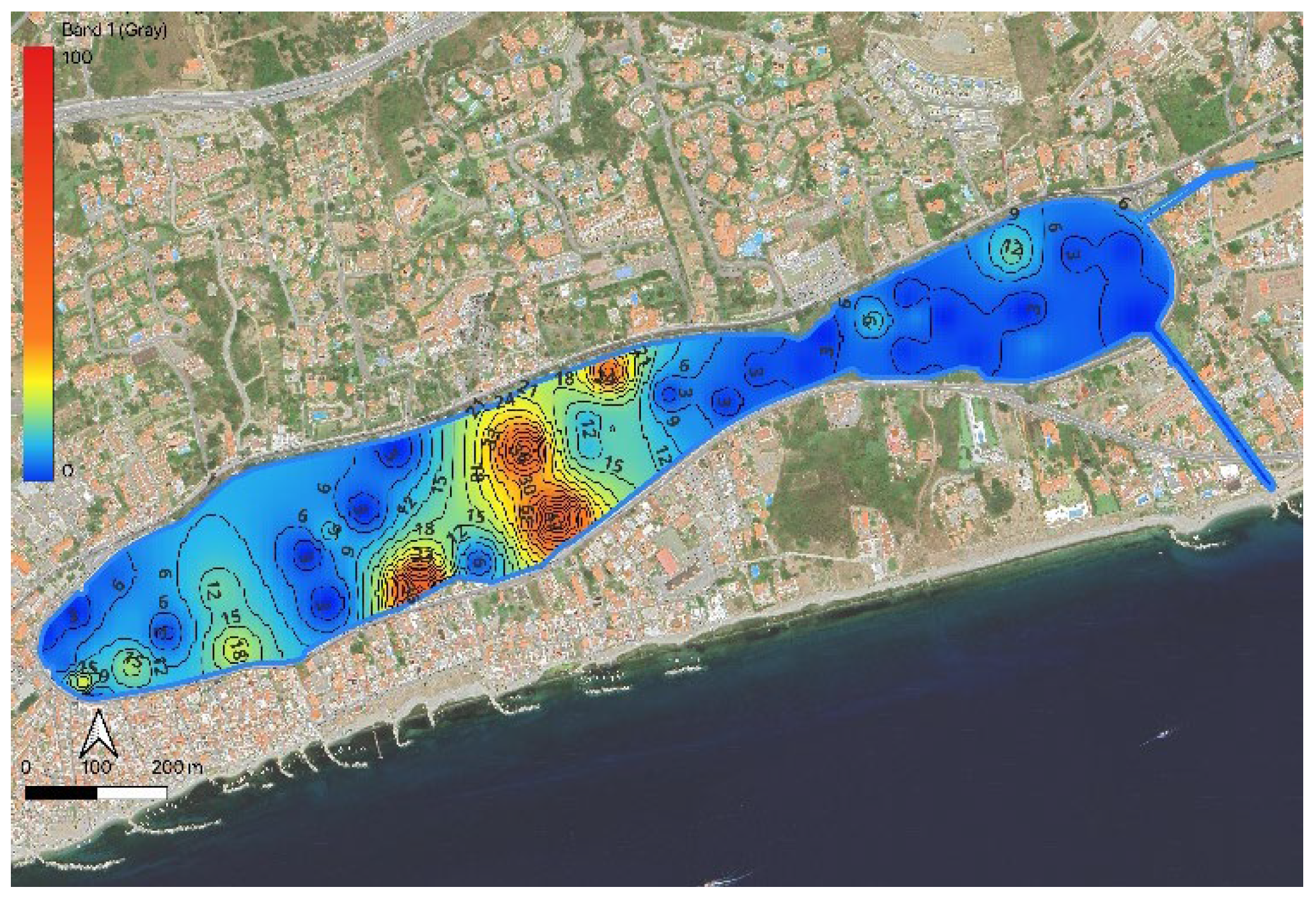
Figure 15.
Sediment samples clustered according to the death assemblage composition. Depth as discriminant factor is put in evidence. The two main clusters recognized by slicing at 40% Bray-Curtis similarity are indicated.
Figure 15.
Sediment samples clustered according to the death assemblage composition. Depth as discriminant factor is put in evidence. The two main clusters recognized by slicing at 40% Bray-Curtis similarity are indicated.
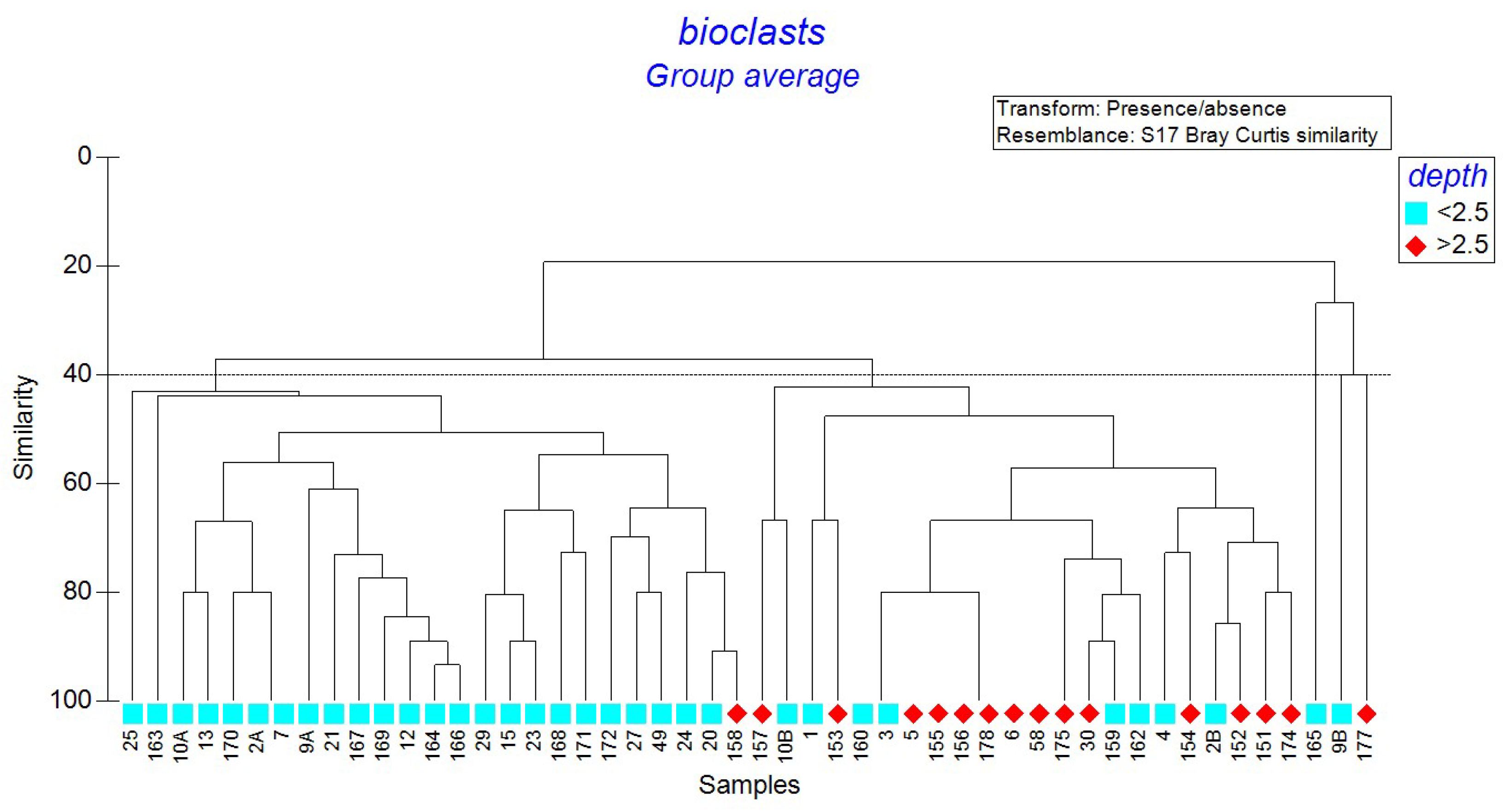
Figure 16.
Geological map of the bottom bed of the Lake Ganzirri, based on QGIS elaborations. The bathymetric contour lines (dotted line) are in meters (spacing: 0.5 m).
Figure 16.
Geological map of the bottom bed of the Lake Ganzirri, based on QGIS elaborations. The bathymetric contour lines (dotted line) are in meters (spacing: 0.5 m).
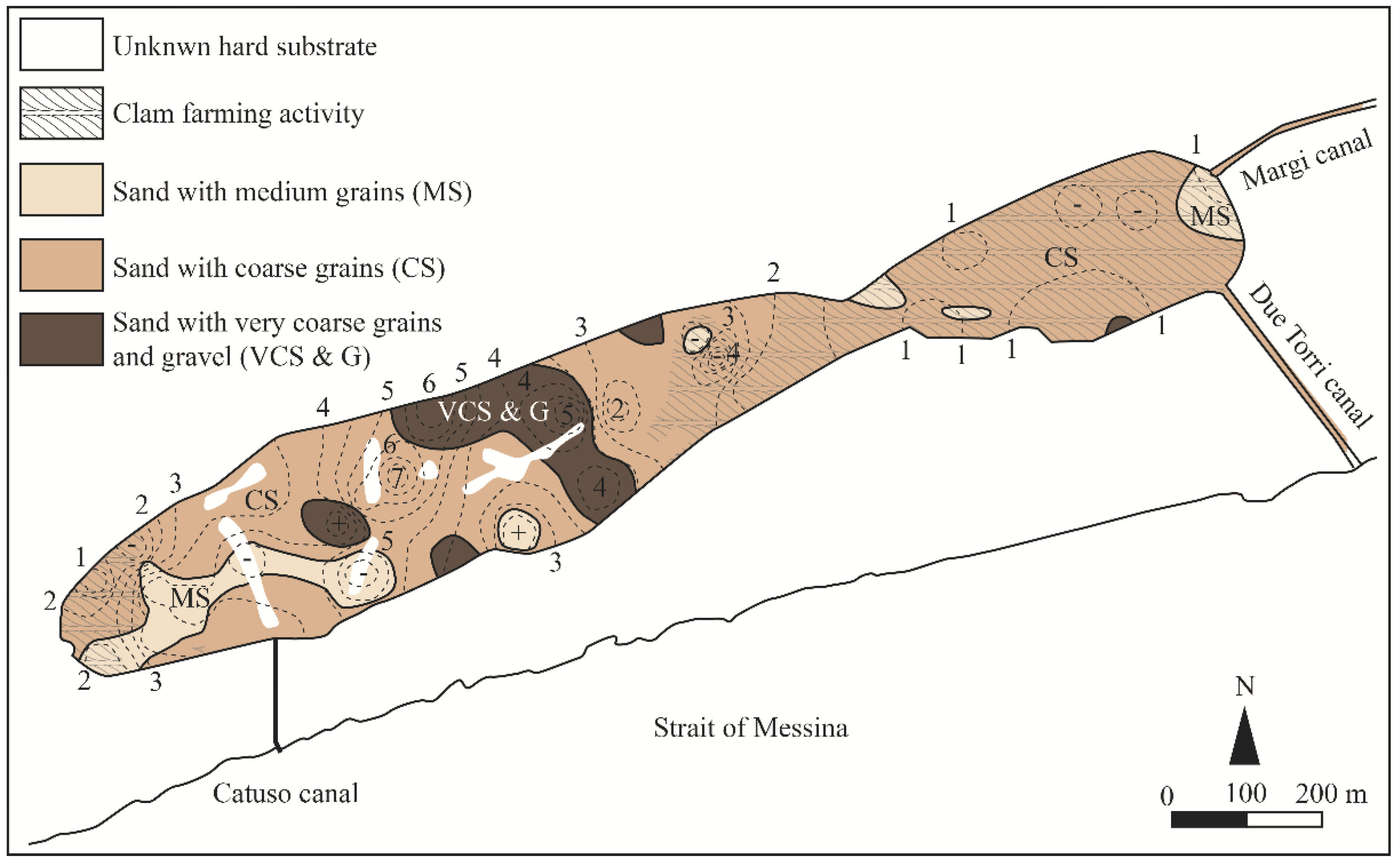
Figure 17.
Synthetic map reconstructing the main heavy metal hotspots (H1–5) in the bottom sediments of the Lake Ganzirri and canals (modified after [15]). The samples (LG) showing the most elevated concentrations were also reported.
Figure 17.
Synthetic map reconstructing the main heavy metal hotspots (H1–5) in the bottom sediments of the Lake Ganzirri and canals (modified after [15]). The samples (LG) showing the most elevated concentrations were also reported.
Disclaimer/Publisher’s Note: The statements, opinions and data contained in all publications are solely those of the individual author(s) and contributor(s) and not of MDPI and/or the editor(s). MDPI and/or the editor(s) disclaim responsibility for any injury to people or property resulting from any ideas, methods, instructions or products referred to in the content. |
© 2026 by the authors. Licensee MDPI, Basel, Switzerland. This article is an open access article distributed under the terms and conditions of the Creative Commons Attribution (CC BY) license.
Copyright: This open access article is published under a Creative Commons CC BY 4.0 license, which permit the free download, distribution, and reuse, provided that the author and preprint are cited in any reuse.


