
Submitted:
15 January 2026
Posted:
16 January 2026
You are already at the latest version
Abstract
Profile conveyor belts are used in operational applications where the transport of bulk materials is required at high inclinations of conveyor belts, typically in the range of 30-40°. The paper deals with the analytical determination of the critical angle of inclination of a homogeneous transverse profile (protrusion), beyond which relative movement of bulk material occurs on the surface of the conveyor belt. The compressive forces induced by the known gravity component of the bulk material acting on a 20 mm high transverse protrusion were experimentally measured on a specially designed laboratory apparatus. The measurements were performed at different inclination angles of the folding plate, which simulated the working surface of the conveyor belt. During the experiments, the investigated bulk material - river gravel with a grain size of 48 mm - was placed in a plastic frame with a width corresponding to the defined loading width of the conveyor belt. On the basis of the measured values of compressive forces, the static coefficient of shear friction in contact of grains of bulk material with two types of surfaces, namely plastic and rubber, was analytically determined. From the experimental data, the mean values of the static shear friction coefficient were determined, which were 0.33 for the plastic surface and 0.48 for the rubber surface, with the orientation of the protrusion perpendicular (90 deg) to the longitudinal axis of the conveyor belt. The experimental investigation also included the determination of the internal friction angle of the river gravel. The results show that when bulk material is conveyed by a profile conveyor belt, it is possible to safely convey material with a cross-sectional height greater than the height of the transverse protrusion, provided that the conveyor inclination angle does not exceed the internal friction angle of the bulk material.
Keywords:
steep conveyor belt transport
; profiled conveyor belt
; rib
; shear friction coefficient
; angle of inclination of the protrusion
1. Introduction
Belt conveyors [1] are continuously operating conveying devices [2] designed for the continuous transport of bulk and piece materials by means of an endless loop of a pulling element, which is a conveyor belt. The advantages of belt conveyors are smooth transport with high conveying capacity [3,4], suitability for transport of virtually all bulk materials, low movement resistance [5,6,7,8,9], noiseless operation, safe and reliable operation [10,11] and simple construction with easy assembly and disassembly. The disadvantages are the large number of rotating parts, the difficulty of transporting abrasive and adhesive materials and the limited angle of inclination of the transport [12,13,14].
Authors Zrnić et al. discuss the history of belt conveyors over the years, up to the development of the modern belt conveyor at the end of the 19th century, in papers [15,16].
Thomas Robns Jr and the Robins Conveying Belt Company published the first known belt engineering handbook in 1917, “Handbook of Conveyor Practice” [17].
The conveyor belt is one of the basic parts of the belt conveyor, it forms an endless element orbiting around the end drums, it performs the function of carrying the conveyed material and at the same time it performs the function of the tensile element, which transfers all the movement resistances [18,19] arising during its circulation [20].
A relatively large number of papers are devoted to the area of damage causes, e.g., [21,22], and joint diagnosis, e.g., [23,24], of conveyor belts. From the research of the articles it can be concluded that it has not been investigated in detail what amount of material the profile conveyor belts are able to convey at transport inclination angles up to 40 deg. In this paper, the authors are concerned with the detection of the applied compressive force on homogeneous profiles, which are named “protrusions”, of profile conveyor belts at different transport inclination angles. The paper also defines the cross-section of the belt filling [m2] (whose height exceeds the height of the protrusion) and the volume [m3] that can be safely transported at a given transport inclination angle [deg] and known mechanical-physical parameters of the transported material (grain size, dynamic angle of repose [25], coefficient of internal friction [26], etc.).
In paper [27], the authors P. Banerjee et al. investigate a machine vision–based technique that is specifically designed for assessing surface wear on cleated conveyor belts across the width and belt thickness.
For belt conveyors of classic construction, conveyor belts [28] with a supporting frame made of textile inserts (P–polyamide, E–polyester, V–viscose, Pvs–polyamide + viscose shear, etc.) or steel ropes [29] (for transferring larger tensions) are used. Conveyor belts with a textile frame [30] consist of a frame consisting of inserts, which is protected on both sides by cover layers and protective edges. In very difficult working conditions, conveyor belts are used whose frame is protected from damage by a bumper [31].
For belt conveyors of special designs [32,33], including steep [34,35] and vertical [36] belt conveyors, structurally modified conveyor belts are used. The design modifications of conveyor belts enable the conveying of bulk materials at inclination angles that exceed the limiting inclination angle of conveying by belt conveyors of conventional design [18]. In practice, profiled conveyor belts and cleated conveyor belts are widespread [32], [37,38,39].
Profile conveyor belts [40,41,42] are used for steep conveying [32,34] of bulk materials with an inclination angle of the conveying route of max. 40 deg. The protrusions on the working surface of a WALTER [43] or CHEVRON [44] profile belt are vulcanised at the same time as the belt, the protrusions (homogeneous profiles) are part of the cover layer.
The lack of a uniform methodology or practical guidance for determining the belt filling cross-section of profile conveyor belts represents a significant complication in practice when theoretically designing the conveying capacity of these steep belt conveyors. This article defines the basic parameters that must be considered when assessing the failure-free transport of bulk materials by profile conveyor belts.
A completely new and so far unpublished solution is the analytical determination of the size of the angle of inclination of the protrusions [deg] of profile conveyor belts, at which the relative movement of the conveyed grains of bulk material occurs in the direction of the width of the conveyor belt.
In the case of profile conveyor belts [43] and [44], the optimal design of the shape and the angle of inclination of the protrusins [deg] can prevent the grains of the bulk material to be conveyed from spilling over the edges of the conveyor belt. If the shape of the protrusions is chosen so that its end parts are parallel to the longitudinal axis of the conveyor belt, then it is ensured that the conveyed material grains will be spread on the conveyor belt over the used loading width b [m]. If the protrusions are inclined to the longitudinal conveyor belt at an angle greater than the [deg] angle, then the material grains will tend to move toward the center of the conveyor belt width.
2. Materials and Methods
When transporting bulk materials by belt conveyors of classic construction [45], the disadvantage is the limited angle of inclination of transport δ [deg] (about 18 deg for inward transport and –12 deg for recession transport). The transport slope is defined mainly by the grain size (granulometric composition) of the transported material [46,47] and the coefficient of friction in the contact surfaces of the material grains with the working surface of the conveyor belt.
The grain size of the bulk material is defined by the shape and size of the individual grains [48]. If the grains of material are close to spherical in shape (so-called rotatable grains), the angle of inclination of the transport must be chosen significantly lower than the angle of inclination of the transport of non-rotatable grains of material.
The coefficient of friction f1 [−] in the contact surfaces of the material grains with the working surface of the conveyor belt is a dimensionless number defined as the ratio between the friction force ( ) and the normal force N [N] (). If the sine component of the conveyed material’s gravity S [N] takes on a value higher, see Figure 1(a); than the frictional force T [N] of the conveyed material against the conveyor belt; relative movement of the material against the working surface of the conveyor belt occurs.
The coefficient of static friction f1 [−], in the contact area of the conveyor belt of the classical construction with the conveyed material, can be expressed according to (1), at the transport inclination .
Assuming they are on the profile conveyor belt [9,10,49] are installed (perpendicular to the longitudinal axis of the conveyor belt) with protrusions of height hR [m], see Figure 1(b), and if the magnitude of the friction force T1 [N] (, where is is the bulk density of the material to be conveyed, the coefficient of the internal friction angle, the angle of internal friction) is greater than the sine component of the gravity of the volume V2 [m3] of the conveyed material (), the force acting on the protrusion is .
If the protrusions with regular spacing are installed in the working branch of the endless loop of the conveyor belt, the total volume V [m3] of the conveyed material can be expressed according to relation (2), if it is taken into account that is the used loading width of the conveyor belt of width B [m] [37] and Θ [deg] is the dynamic spreading angle of the conveyed material.
The volume of the conveyed material V2 [m3], see Figure 1(b), can be expressed according to equation (5), assuming the height (see Figure 2(b)).
When the protrusions are inclined by an angle [deg] to the longitudinal axis of the profile conveyor belt (i.e., an angle α [deg] to the transverse axis of the folding Plexi plate of the laboratory device), see Figure 3(a), a normal force acts on the protrusion and frictional force acts in the contact area between the protrusion and the conveyed material. If the magnitude of the force F2 [N] is less than the magnitude of the friction force T2 [N], there is no relative movement of the conveyed material layer with respect to the working surface of the conveyor belt in the direction of the “u” axis (see Figure 3(a)).
The equation of motion (6) in the direction of the “u” axis can be expressed according to Figure 3(a).
The equation (6) can be modified to the form (7) provided that , , .
Solving the quadratic equation (7), the maximum size of the angle can be found [deg] (8), at which the material to be conveyed does not yet start to slide in the direction of the “u” axis on the working surface of the profile conveyor belt.
Table 1 shows the values of the [deg] protrusion inclination angle (see Figure 3(b) and Figure 3(c)) calculated according to equation (8) at a transport inclination angle and a shear friction coefficient f1 [−].

Table 1.
Angle of protrusion inclination [deg] and coefficient k [–] at the transport inclination angle [deg] and shear friction coefficient f1 = 0.3.
Table 1.
Angle of protrusion inclination [deg] and coefficient k [–] at the transport inclination angle [deg] and shear friction coefficient f1 = 0.3.
| Kinetic friction f1 = 0.3 | ||||||||||
|---|---|---|---|---|---|---|---|---|---|---|
| δ1 [deg] | 18 | 20 | 22 | 24 | 26 | 28 | 30 | 34 | 34 | 36 |
| [deg] 1 | 11.13 | 21.16 | 27.97 | 33.11 | 37.20 | 40.59 | 43.45 | 45.92 | 48.09 | 50.00 |
| α [deg] | 78.87 | 68.84 | 62.03 | 56.89 | 52.80 | 49.41 | 46.55 | 44.08 | 41.91 | 40.00 |
| k [–] 1 | 0.924 | 0.824 | 0.743 | 0.674 | 0.615 | 0.564 | 0.52 | 0.48 | 0.445 | 0.413 |
1 see Figure 4.
Figure 4.
Angle of protrusion inclination [deg] and coefficient k [–] at the transport inclination angle [deg] and a shear friction coefficient f1 [−].
Figure 4.
Angle of protrusion inclination [deg] and coefficient k [–] at the transport inclination angle [deg] and a shear friction coefficient f1 [−].
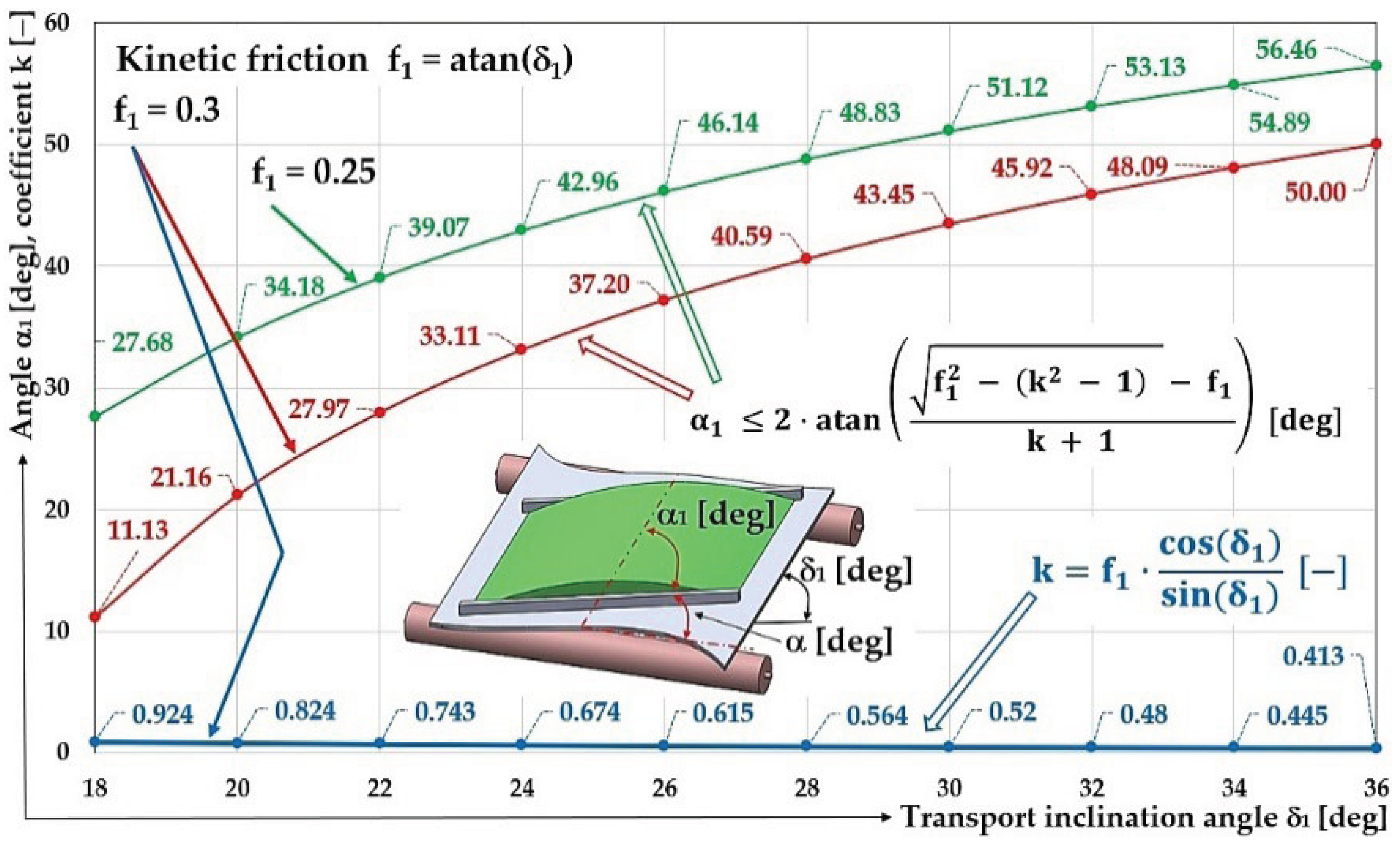
Table 2.
Angle of protrusion inclination [deg] and coefficient k [–] at the transport inclination angle [deg] and shear friction coefficient f1 = 0.25.
Table 2.
Angle of protrusion inclination [deg] and coefficient k [–] at the transport inclination angle [deg] and shear friction coefficient f1 = 0.25.
| Kinetic friction f1 = 0.25 | ||||||||||
|---|---|---|---|---|---|---|---|---|---|---|
| δ1 [deg] | 18 | 20 | 22 | 24 | 26 | 28 | 30 | 34 | 34 | 36 |
| [deg] 1 | 27.68 | 34.18 | 39.07 | 42.96 | 46.14 | 48.83 | 51.12 | 53.13 | 54.89 | 56.46 |
| α [deg] | 62.32 | 55.82 | 50.93 | 47.04 | 43.86 | 41.17 | 38.88 | 36.87 | 35.11 | 33.54 |
| k [–] | 0.769 | 0.687 | 0.619 | 0.562 | 0.513 | 0.47 | 0.433 | 0.4 | 0.371 | 0.344 |
1 see Figure 4.
In order to be able to obtain accurate values of the applied compressive force on the transverse protrusion inclined to the longitudinal axis of the folding plate by an angle [deg], a laboratory device was designed and constructed, see Figure 5, which consists of three basic parts I – the folding plate (inclination angle with respect to the horizontal plane), II – the supporting frame and III – the strain gauge load sensor PW2G C3–12 kg [52], detecting the magnitude of the compressive forces and .
On the inclined surface (at a predetermined angle of inclination to the horizontal ) of the laboratory equipment 1, see Figure 6, a PLEXI frame was placed 2 of gravity = 3.26 N (weight = 0.332 kg), into which the bulk material was placed 3 of known gravity . The applied compressive force on the transverse protrusion from the Plexi frame and also from the gravity component of the bulk material (river gravel, grain size 4 ÷ 8 mm) was detected by a load sensor 4 [52] at a known value of the inclination angle [deg] of the folding plate.
To determine the coefficient of internal friction angle of the bulk material [−], laboratory tests were carried out as follows. A 1st plastic frame was placed on the working surface (Plexi or rubber) of the folding plate, slowly deflected by an angle [deg] to the horizontal plane. The inner space of this plastic frame was completely filled with loose material of known gravity [N].
A 2nd plastic frame was placed on top of the 1st plastic frame and a batch of bulk material of known gravity [N] was slowly poured into it.
The lower plastic frame met the transverse protrusion with its front surface. In the contact area (corresponding to the plane parallel to the surface of the folding plate of the laboratory equipment, spaced by the height of the lower frame [m]), the material grains of the bulk material placed in the lower frame came into contact with the material grains placed in the upper frame.
If the gravity component of the bulk material charge [N] has taken on a magnitude greater than the frictional force [N] (acting in the contact area of the shear plane), relative movement of the upper frame relative to the lower frame has occurred. The angle [deg] is considered to be the angle of internal friction of the bulk material (river gravel, rounded grain edges). By substituting the value [deg] into equation (1), the coefficient of the internal friction angle of the bulk material [−] can be analytically calculated.
A load sensor cable equipped with a D-Sub plug 5 was plugged into the socket of the measuring module BR4-D 6 [53] of the strain gauge apparatus DS NET during the laboratory measurements. A PC 9 (ASUS K72JR–TY131 laptop) was connected to the DS NET strain gauge 7 using a network cable with RJ–45 connectors 8 at both ends.
3. Results
From the values detected by the load sensor [52] in the DEWESoft X software environment [54], with the known value of the material gravity G [N] and the inclination angle of the folding plate [deg], the friction coefficient was calculated according to equation (8), where “i” defines the surface of the folding plate i = P for Plexi, i = R for rubber.
3.1. Contact Surface Plexi, Inclination of Protrusion α = 0 deg
This section may be divided by subheadings. It should provide a concise and precise description of the experimental results, their interpretation, as well as the experimental conclusions that can be drawn.
Table 3 presents the measured values of the pressure forces , a acting on the protrusion at the angle of inclination of the folding plate a .
The quantity expresses the force detected by the load sensor [52] at the moment of the start of the measurement. The non-zero magnitude of the compressive force is due to the fact that the load sensor [52] was calibrated (with a calibrated 2 kg weight load) in the horizontal position, without the fasteners used and without the plastic plate (500 mm long, 20 mm high and 5 mm thick) that simulates the transverse protrusion.
The pressure force defines the force generated by a Plexi frame (weight 0.332 kg, gravity 3.26 N) placed on the surface of the folding plate on the load sensor [52].
Loose material (river gravel of 4÷8 mm grain size) of known gravity is poured into the inner space of the Plexi frame . In the DEWESoft software environment, the magnitude of the force , acting on the load sensor [52], from the gravity component of the bulk material is recorded.
From the measured values of the forces , and and the known value of the gravity of the bulk material, the actual magnitude of the compressive force acting on the protrusion from the gravity component of the bulk material was calculated. From this force , the gravity of the bulk material and the angle of inclination of the folding Plexi plate, the shear friction coefficient was calculated according to equation (8).
Table 3.
Measured values , , at transport inclination angle = 18 deg and 23 deg and protrusion inclination angle α = 0 deg.
Table 3.
Measured values , , at transport inclination angle = 18 deg and 23 deg and protrusion inclination angle α = 0 deg.
| δ1 | [deg] | 18 | 23 | ||||||||||
|---|---|---|---|---|---|---|---|---|---|---|---|---|---|
| k | G | F0M(18),k | FFM(18),k | FF(18),k | FM(18),k | F(18,0),k | f1P(18,0),k | F0M(23),k | FFM(23),k | FF(23),k | FM(23),k | F(23,0),k | f1P(23,0),k |
| [N] | [N] | [N] | [N] | [N] | [N] | [–] | [N] | [N] | [N] | [N] | [N] | [–] | |
| 1 | 70 | −0.411 | 0.281 | 0.691 | 2.981 | 3.111 | 0.28 | −0.382 | 1.272 | 1.652 | 8.142 | 7.252 | 0.31 |
| 2 | 70 | −0.28 | 0.29 | 0.57 | 3.17 | 3.16 | 0.28 | −0.26 | 1.13 | 1.39 | 8.43 | 7.56 | 0.31 |
| 3 | 70 | −0.36 | 0.28 | 0.64 | 3.04 | 3.12 | 0.28 | −0.31 | 1.18 | 1.49 | 7.96 | 7.09 | 0.31 |
| f1P(18,0)AM = | 0.28 | f1P(23,0)AM = | 0.31 | ||||||||||
| κ(5%,3)18 = | ± 0.00 | κ(5%,3)23 = | ± 0.00 | ||||||||||
From three times (n = 3) repeated measurements under the same technical conditions, the arithmetic mean and the marginal error (9) were calculated according to Student’s distribution [55].
where is the Student’s coefficient (for the chosen risk β = 5% and the number of measured values can be determined according to [55] ); is the standard deviation of the arithmetic mean (10).
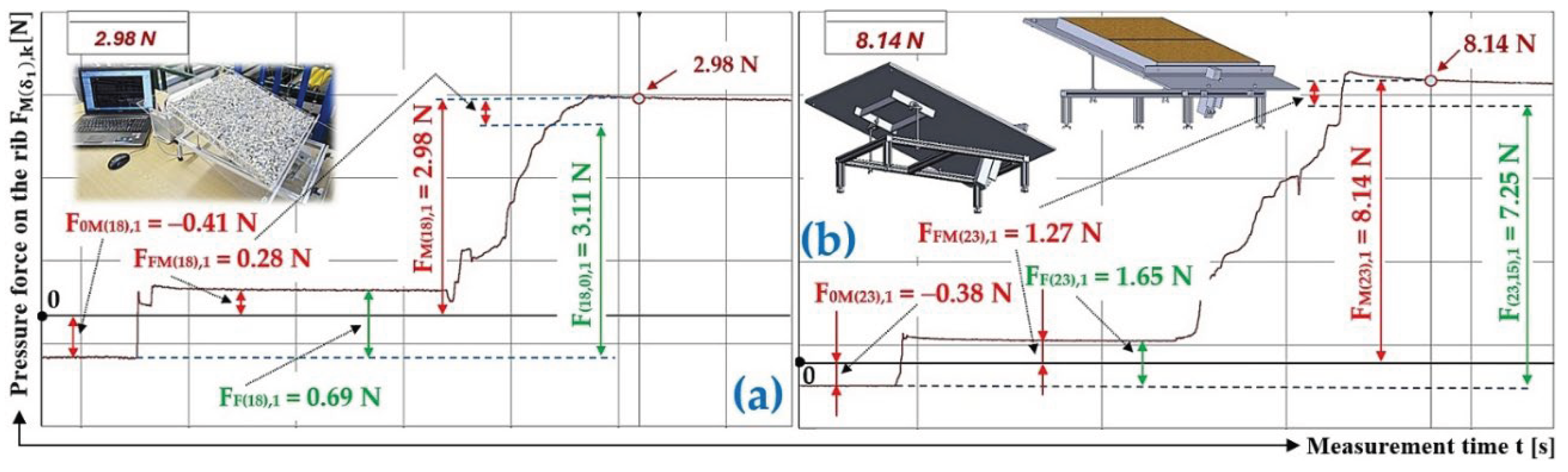
Figure 7(a) presents the time history of the measured compressive force by the load sensor [52], generated by a bulk material of known gravity G = 70 N, distributed on the surface of a folding Plexi plate inclined to the horizontal plane by an angle δ1 = 18 deg. The Plexi plate (simulating the protrusion) is inclined at an angle = 90 deg to the longitudinal axis of the folding Plexi plate, i.e., at an angle α = 0 deg to the transverse axis (width b = 400 mm) of the folding Plexi plate.
Time history of the compressive force (a batch of bulk material with a gravity of G = 70 N) detected by the load sensor [52] at an angle of inclination of the Plexi plate = 23 deg is indicated in Figure 7(b).
Figure 7.
Measured value of pressure force in the DeweSoft software environment for a protrusion angle of α = 0 deg and a conveyor belt inclination angle of (a) = 18 deg, (b) = 23 deg.
Figure 7.
Measured value of pressure force in the DeweSoft software environment for a protrusion angle of α = 0 deg and a conveyor belt inclination angle of (a) = 18 deg, (b) = 23 deg.
The magnitude of three times the measured compressive force of the bulk material of gravity G = 70 N acting on the protrusion (located at an angle = 90 deg to the longitudinal axis, i.e., α = 0 deg to the transverse axis) of the folding plate, deflected by an angle = 28 deg and = 32 deg from the horizontal plane, is given in Table 4.
Time history of the compressive force (a batch of bulk material with a gravity of G = 70 N) detected by the load sensor [52] at a Plexi plate inclination angle (simulating a conveyor belt) = 23 deg and a lug inclination angle = 90 deg with respect to the longitudinal axis (α = 0 deg with respect to the transverse axis) of the folding plate, is indicated in Figure 8.
The measured values , , by the load sensor [52]; acting on the Plexi plate (simulating the transverse protrusion) of the laboratory device (see Figure 5); are (for the inclination angle of the folding plate and the inclination angle of the protrusion ) shown in Table 5.
Figure 9(a) presents the time history of the measured compressive force of a bulk material of gravity G = 70 N, spread on the surface of a folding Plexi plate inclined to the horizontal plane at an angle = 32 deg.
3.2. Contact Surface Plexi, Inclination of Protrusion α = 15 deg
Measurement of the quantity; which is the compressive force of the bulk material of gravity G [N] acting on a transverse Plexi plate of height 20 mm (simulating a transverse protrusion), placed at an angle α = 15 deg to the transverse axis (i.e., = 75 deg to the longitudinal axis) of the folding plate (simulating a conveyor belt); by a precision instrument (strain gauge load sensor PW2G C3–12 kg) and carefully repeated under the same conditions does not yield the same values. However, the measurand has one actual (accurate) value for the given measurement conditions.
Table 6 shows the measured values of the compressive forces ,, (of bulk material of gravity G = 45 N acting on the Plexi plate, mechanically attached to the load sensor [52] at an angle α = 15 deg with respect to the transverse axis of the folding Plexi plate) of three times repeated measurements for the inclination angle of the folding plate = 18 deg and = 23 deg. From these measured forces, the arithmetic mean and the extreme error are calculated according to equation (9).
Figure 10(a) presents the time history of the measured compressive force by the load sensor [52], generated by a bulk material of known gravity G = 45 N, distributed on the surface of a folding Plexi plate inclined to the horizontal plane by an angle = 18 deg. The Plexi plate (simulating the protrusion) is inclined at an angle α = 0 deg to the transverse axis of the folding Plexi plate.
Time history of the compressive force (a batch of bulk material with a gravity of G = 45 N) detected by the load sensor [52] at an angle of inclination of the Plexi plate = 23 deg is indicated in Figure 10(b).
The magnitude of three times the measured compressive force of the bulk material of gravity G = 70 N acting on the protrusion (located at an angle α = 15 deg to the transverse axis) of the folding plate, deflected by an angle = 28 deg and = 32 deg from the horizontal plane, is given in Table 7.
Figure 11(a) presents the time history of the measured compressive force by the load sensor [52], generated by a bulk material of known gravity G = 45 N, distributed on the surface of a folding Plexi plate inclined to the horizontal plane by an angle = 28 deg. The Plexi plate (simulating the protrusion) is inclined at an angle α = 15 deg to the transverse axis of the folding Plexi plate.
Time history of the compressive force (a batch of bulk material with a gravity of G = 45 N) detected by the load sensor [52] at an angle of inclination of the Plexi plate = 32 deg is indicated in Figure 11(b).
The measured values , , by the load sensor [52]; acting on the Plexi plate (simulating the transverse protrusion) of the laboratory device (see Figure 5); are (for the inclination angle of the folding plate and the inclination angle of the protrusion ) shown in Table 8.
Time history of the compressive force (a batch of bulk material with a gravity of G = 45 N) detected by the load sensor [52] at a Plexi plate inclination angle (simulating a conveyor belt) = 38 deg and a lug inclination angle α = 15 deg with respect to the transverse axis of the folding plate, is indicated in Figure 12.
3.3. Contact Surface Rubber, Inclination of Protrusion α = 0 deg
Table 9 shows the measured values of the compressive forces ,, (of bulk material of gravity G = 70 N (G = 41 N) acting on the Plexi plate, mechanically attached to the load sensor [52] at an angle α = 0 deg with respect to the transverse axis of the folding Plexi plate) of three times repeated measurements for the inclination angle of the folding plate = 18 deg ( = 23 deg). From these measured forces, the arithmetic mean and the extreme error are calculated according to equation (9).
Figure 13(a) presents the time history of the measured compressive force by the load sensor [52], generated by a bulk material of known gravity G = 70 N, distributed on the surface of a folding Plexi plate inclined to the horizontal plane by an angle = 18 deg. The Plexi plate (simulating the protrusion) is inclined at an angle α = 0 deg to the transverse axis of the folding Plexi plate.
Time history of the compressive force (a batch of bulk material with a gravity of G = 41 N) detected by the load sensor [52] at an angle of inclination of the Plexi plate = 23 deg is indicated in Figure 13(b).
The magnitude of three times the measured compressive force of the bulk material of gravity G = 41 N acting on the protrusion (located at an angle α = 0 deg to the transverse axis) of the folding plate, deflected by an angle = 28 deg and = 32 deg from the horizontal plane, is given in Table 10.
Figure 14(a) presents the time history of the measured compressive force by the load sensor [52], generated by a bulk material of known gravity G = 41 N, distributed on the surface of a folding Plexi plate inclined to the horizontal plane by an angle = 28 deg. The Plexi plate (simulating the protrusion) is inclined at an angle α = 0 deg to the transverse axis of the folding Plexi plate.
Time history of the compressive force (a batch of bulk material with a gravity of G = 41 N) detected by the load sensor [52] at an angle of inclination of the Plexi plate = 32 deg is indicated in Figure 14(b).
The measured values , , by the load sensor [52]; acting on the Plexi plate (simulating the transverse protrusion) of the laboratory device (see Figure 5); are (for the inclination angle of the folding plate and the inclination angle of the protrusion ) shown in Table 11.
Time history of the compressive force (a batch of bulk material with a gravity of G = 70 N) detected by the load sensor [52] at a Plexi plate inclination angle (simulating a conveyor belt) = 38 deg and a lug inclination angle α = 0 deg with respect to the transverse axis of the folding plate, is indicated in Figure 15.
3.4. Contact Surface Rubber, Inclination of Protrusion α = 15 deg
Table 12 shows the measured values of the compressive forces ,, (of bulk material of gravity G = 41 N) acting on the Plexi plate, mechanically attached to the load sensor [52] at an angle α = 15 deg with respect to the transverse axis of the folding Plexi plate) of three times repeated measurements for the inclination angle of the folding plate = 23 deg ( = 28 deg). From these measured forces, the arithmetic mean and the extreme error are calculated according to equation (9).
Figure 16(a) presents the time history of the measured compressive force by the load sensor [52], generated by a bulk material of known gravity G = 41 N, distributed on the surface of a folding Plexi plate inclined to the horizontal plane by an angle = 23 deg. The Plexi plate (simulating the protrusion) is inclined at an angle α = 15 deg to the transverse axis of the folding Plexi plate.
Time history of the compressive force (a batch of bulk material with a gravity of G = 41 N) detected by the load sensor [52] at an angle of inclination of the Plexi plate = 28 deg is indicated in Figure 16(b).
The magnitude of three times the measured compressive force of the bulk material of gravity G = 41 N acting on the protrusion (located at an angle α = 15 deg to the transverse axis) of the folding plate, deflected by an angle = 32 deg and = 38 deg from the horizontal plane, is given in Table 13.
Figure 17(a) presents the time history of the measured compressive force by the load sensor [52], generated by a bulk material of known gravity G = 41 N, distributed on the surface of a folding Plexi plate inclined to the horizontal plane by an angle = 32 deg. The Plexi plate (simulating the protrusion) is inclined at an angle α = 15 deg to the transverse axis of the folding Plexi plate.
Time history of the compressive force (a batch of bulk material with a gravity of G = 41 N) detected by the load sensor [52] at an angle of inclination of the Plexi plate = 88 deg is indicated in Figure 17(b).
Table 14 shows the mean values , calculated according to the equation (8) of the shear friction coefficients of bulk material (river gravel of grain size 4÷8 mm) in the contact surface of the folding plate, inclined at an angle [deg].
Figure 18 shows the calculated values, according to the equation (8), of the shear friction coefficient of the bulk material (river gravel of 4÷8 mm grain size) in the contact area (j = P − Plexi, j = R −rubber) of the folding plate inclined at an angle [deg].
3.5. Determination of the Coefficient of Internal Friction of Bulk Material
Figure 19(a) shows the method of measurement on the laboratory equipment to determine the angle of inclination [deg] at which the movement of a volume of a batch of bulk material spread inside the upper frame will occur 2, relative to the bulk material inside the lower frame 1.
This section may be divided by subheadings. It should provide a concise and precise description of the experimental results, their interpretation, as well as the experimental conclusions that can be drawn.
Figure 19(b) presents the measured inclination angle = 29.4 deg of the folding plate of the laboratory device, at which the movement of the bulk batch of bulk material spread inside the upper frame relative to the bulk material placed in the lower frame began.
Table 15 shows the measured values of the inclination angle [deg] of the folding plate of the laboratory device at which the relative motion of the upper frame 1, see Figure 19(a), to the lower frame 2 began. From these five times (n = 5) repeated measurements of the inclination angle [deg] under the same technical conditions, the magnitudes of the internal friction angle coefficient [–] were calculated according to the equation (1) (for the number of measurements k = 1 to n). From the calculated magnitudes of the coefficients of the internal friction angle [–], the arithmetic mean [–] and the extreme error were calculated according to the equation (9). For the chosen risk β = 5% and the number of measured values , the Student’s coefficient can be determined according to [55].
4. Discussion
From the values obtained by measuring the pressure forces acting on a transverse protrusion inclined by an angle [deg] with respect to the longitudinal (α [deg] transverse) axis of the folding Plexi plate (simulating a section of the conveyor belt between two adjacent protrusions), it follows that at low angles of inclination [deg] of the folding Plexi plate, the magnitude of the coefficient takes on a lower value than in the case of higher angles of inclination [deg] of the folding Plexi plate. This fact can be expressed by the fact that the friction force in the contact area of the conveyed material grains with the folding Plexi plate takes a value higher than the sine component of the gravity of the conveyed material. The friction force T [N] prevents the relative (backward) movement of the material against the direction of movement of the conveyor belt. At low angles of inclination [deg] of the conveyor belt, there is no backward movement of the conveyed material even if no transverse protrusion are installed on the conveyor belt.
If a bulk material of gravity G [N] is in contact with the Plexi (j = P) surface of the folding plate (simulating the working surface of the conveyor belt) at an angle of inclination of the protrusion α = 0 deg and an angle of the folding plate (), the friction coefficient takes the value (). Both these friction coefficient values are not the actual value of the friction coefficient of the bulk material (river gravel) against the Plexi surface of the folding plate. The actual magnitude of the friction coefficient corresponds to the condition where the friction force in the contact surface of the material grains conveyed with the Plexi surface of the folding plate (inclined to the horizontal plane by an angle ), takes a value lower than the sine component of the gravity of the material conveyed.
If the bulk material is placed on the rubber (j = R) surface of the folding plate, then when the angle of inclination of the protrusion α = 0 deg and the inclination of the folding plate , () the friction coefficient takes the value ( and ). These three values of the coefficient of friction are not the actual value of the coefficient of friction of the loose material (river gravel) against the rubber surface of the folding plate. The actual magnitude of the coefficient of friction is which corresponds to the condition where the friction force in the contact surface of the material grains conveyed with the rubber surface of the folding plate (inclined to the horizontal plane by an angle ), takes a value lower than the sine component of the gravity of the material conveyed.
In the case that a bulk material of gravity G [N] is placed on the Plexi surface of the folding plate; the friction coefficient takes the value ( and ) when the angle of inclination of the protrusion α = 15 deg and the angle of inclination of the folding plate , ( and );. These three friction coefficient values are again not the actual value of the friction coefficient of the bulk material (river gravel) against the plastic surface of the folding plate. The actual magnitude of the friction coefficient is .
If the bulk material is placed on the rubber (j = R) surface of the folding plate, then with the angle of inclination of the protrusion α = 15 deg and the inclination of the folding plate , () the friction coefficient takes the value (). These two values of the coefficient of friction are not the actual value of the coefficient of friction of the bulk material (river gravel) against the rubber surface of the folding plate. The actual magnitude of the coefficient of friction is which corresponds to the condition where the friction force in the contact surface of the material grains conveyed with the rubber surface of the folding plate (inclined to the horizontal plane by an angle ), takes a value lower than the sine component of the gravity of the material conveyed.
The static coefficient of internal friction angle of a bulk material [46] is a basic mechanical characteristic of bulk materials that describes the resistance of a material to shear between its particles at rest [47,48]. For the loose material river gravel (dry, rounded grains) the coefficient of the internal friction angle takes the value = 0.45 ÷ 0.65 [56,57]. The measurements carried out on the laboratory equipment, see chapter 3.5, show that the mean value of the static coefficient of the internal friction angle of the bulk material - dry river gravel - takes the value = 0.54.
The internal friction angle of a bulk material is influenced by a number of factors related to the properties of the particles and their arrangement. The granulometry (shape and grain size) of the bulk material, moisture, compaction and the method of loading have a major influence on the magnitude of the internal friction angle. Given the operating conditions characterised by dynamic loads and vibrations under which profile conveyor belts are commonly used, the limiting angle of inclination of the conveyor, at which the grains of the conveyed material move against the direction of movement of the conveyor belt, can be expected to be lower than the angle 28 deg. The difference between the static and dynamic angle of internal friction, resulting from the state of particle motion and the magnitude of frictional resistance of the bulk material conveyed by the profile belt, must be taken into account when determining the operating conditions for a particular type of material and its mechanical-physical properties.
5. Conclusions
At present, there is no clear way to determine the cross-section of the belt fill or to determine theoretically the quantity of bulk material that can be moved per unit time by profile conveyor belts inclined at a certain angle to the horizontal plane. The aim of the article was to describe and analyse the key parameters that need to be taken into account when transporting bulk materials by belt conveyors fitted with profile conveyor belts.
This paper describes a laboratory device that simulates a section of a conveyor belt between two adjacent transverse protrusions. A strain gauge load sensor PW2G-C3 with a measuring range of 0 ÷ 12 kg is attached to the folding plate of the experimental device, which senses the magnitude of the applied compressive force of the bulk material (river gravel with a grain size of 4 mm ÷ 8 mm) on the transverse protrusion at different inclination angles of the folding plate of the laboratory device.
From the measured pressure force acting on the transverse protrusion, the known value of the inclination angle of the folding plate and the gravity of the bulk material, the shear friction coefficient in the contact area of the material grains with the surface (Plexi or rubber) of the folding plate is analytically calculated.
If the conveyor belt is equipped with a profile conveyor belt uniformly filled with bulk material in the horizontal section, then when the conveyor belt is guided along the inclined section of the conveyor belt, the material grains do not spill over the transverse protrusions of a lower height than the height of the bulk material layer carried on the working surface of the profile conveyor belt. This fact can be expressed by the fact that the coefficient of the internal friction angle [−] (the coefficient of shear friction between individual grains of bulk material in a plane a height [m] away from the conveyor belt surface) is higher than the coefficient of shear friction between the material grains [−] (the coefficient of the external friction angle) and the conveyor belt working surface.
Overfilling of the layer of material grains located above the plane of the height [m] of the transverse protrusion occurs when the angle of inclination of the profile belt becomes .
The protrusions on the working surface of profile conveyor belts are usually realized by the manufacturers in the shape of a V, where one arm of the “V” protrusion is at an angle [deg] with the longitudinal axis of the conveyor belt. In the paper, the calculation of the angle of inclination of the protrusion arm is performed, at which there is no relative movement of the bulk material in the lateral direction of the conveyor belt (material grains do not spill over the lateral edge of the profile conveyor belt) at the angle of inclination of the transport.
Author Contributions
Conceptualization, L.H.; methodology, L.H.; software, L.H.; validation, L.H., J.B. and L.V.; formal analysis, L.H. and L.K.; investigation, L.H. and J.B.; resources, L.H.; data curation, L.K.; writing—original draft preparation, L.H.; writing—review and editing, L.H.; visualization, L.H.; supervision, J.B. and L.K.; project administration, L.H.; funding acquisition, L.H. All authors have read and agreed to the published version of the manuscript.
Funding
This research was funded by “Research and development of smart processes in industrial practice”, grant number SP2026/001 and was funded by MŠMT ČR (Ministry of Education Youth and Sports).
Institutional Review Board Statement
Not applicable.
Informed Consent Statement
Not applicable.
Data Availability Statement
Measured data of effective vibration speed values iRMS(α,β,m,ne) [mm·s−1], listed from Table 3, Table 4, Table 5, Table 6, Table 7, Table 8, Table 9, Table 10, Table 11, Table 12 and Table 13 and processed using DEWESoft X software, can be sent in case of interest, by prior written agreement, in *.XLSX (Microsoft Excel) format.
Conflicts of Interest
The authors declare no conflict of interest. The funders had no role in the design of the study; in the collection, analyses, or interpretation of data; in the writing of the manuscript; or in the decision to publish the results.
References
- Yardley, E.; David; STACE, L. Rod. Belt conveying of minerals, 1st ed.; Publisher: Elsevier, UK, 2008; p. 200. ISBN 19781845694302. [Google Scholar]
- Bajda, M.; Hardygóra, M. Analysis of the Influence of the Type of Belt on the Energy Consumption of Transport Processes in a Belt Conveyor. Energies 2021, 14(19), 6180. [Google Scholar] [CrossRef]
- Semenchenko, A.; Stadnik, M.; Belitsky, P.; Semenchenko, D.; Stepanenko, O. The impact of an uneven loading of a belt conveyor on the loading of drive motors and energy consumptlt conveying of mineron. Вoстoчнo-Еврoпейский журнал передoвых технoлoгий 2016, 4(1), 42–51. [Google Scholar] [CrossRef]
- Tsakalakis, K.G.; Micalakopoulos, Th. Mathematical modelling of the conveyor belt capacity. In Proceedings of the 8th International Conference for Conveying and Handling of Particulate Solids, Tel–Aviv, Israel, May 2015; 2015. [Google Scholar]
- Wheeler, C.A. Predicting the main resistance of belt conveyors. In Proceedings of the International Materials Handling Conference Beltcon 12, Johannesburg, South Africa, 23−24 July 2003; Available online: https://beltcon.org.za/wp-content/uploads/2024/12/B12-08-Wheeler.pdf.
- Bajda, M.; Krol, R. Experimental tests of selected constituents of movement resistance of the belt conveyors used in the underground mining. Procedia Earth and Planetary Science 2015, 15, 702–711. [Google Scholar] [CrossRef]
- Munzenberger, P.; Wheeler, C. Laboratory measurement of the indentation rolling resistance of conveyor belts. Measurement 2016, 94, 909–918. [Google Scholar] [CrossRef]
- Gładysiewicz, L.; Konieczna, M. Theoretical basis for determining rolling resistance of belt conveyors, 1st ed.; Wroclaw University of Science and Technology: Poland, 2016; p. 105−119. ISSN 2300-9586. [Google Scholar]
- Beh, B.; Wheeler, C.A.; Munzenberger, P. Analysis of conveyor belt flexure resistance. Powder Technology 2019, 357, 158–163. [Google Scholar] [CrossRef]
- Li, M.; Yingqian, S.U.N.; Luo, C. Reliability analysis of belt conveyor based on fault data. In Proceedings of the 5th International Conference on Mechanical Engineering and Automation Science (ICMEAS 2019), Wuhan, China, 10–12 October 2019. [Google Scholar] [CrossRef]
- Zhang, S.; Xia, X. Optimal control of operation efficiency of belt conveyor systems. Applied Energy 2010, 87(6), 1929–1937. [Google Scholar] [CrossRef]
- Kiriia, R.; Smirnov, A.; Zhyhula, T.; Zhelyazov, T. Determination of the limiting angle of inclination of tubular belt conveyor. II International Conference Essays of Mining Science and Practice. E3S Web of Conferences 168; 2020; p. 00047 EDP Sciences. [Google Scholar] [CrossRef]
- Ananth, K.N.S.; Rakesh, V.; Visweswarao, P. K. Design and selecting the proper conveyor-belt. International Journal of Advanced Engineering Technology 2013, 4(2), 43–49. [Google Scholar]
- Dos Santos, J.A. Theory and design of Sandwich Belt High Angle Conveyors according to the Expanded Conveyor Technology. Bulk Solids Handling 2000, 20(1), 27–38. [Google Scholar]
- Zrnić, N.; Đorđević, M.; Gašić, V. History of Belt Conveyors Until the End of the 19th Century. In Explorations in the History and Heritage of Machines and Mechanisms. HMM 2022. History of Mechanism and Machine Science; Ceccarelli, M., López-García, R., Eds.; Springer: Cham; vol 40. [CrossRef]
- Zrnić, N.; Đorđević, M.; Gašić, V. Historical Background and Evolution of Belt Conveyors. Found Sci 2024, 29, 225–255. [Google Scholar] [CrossRef]
- Robins, T. Handbook of conveyor practice, 1st ed.; Alspaugh Engineering LCC: Chicago, USA, 1917; Available online: https://www.alspaugh-engineering.com/blog-3/blog-post-title-one-f4bm5.
- ISO 5048 Continuous mechanical handling equipment – Belt conveyors with carrying idlers – Calculation of operating power and tensile forces. ISO/TC 01. 1989; 12. Available online: https://www.iso.org/standard/11069.html.
- Bajda, M.; Hardygóra, M. Analysis of reasons for reduced strength of multiply conveyor belt splices. Energies 2021, 14(5), 1512. [Google Scholar] [CrossRef]
- Bortnowski, P.; Kawalec, W.; Król, R.; Ozdoba, M. Identification of conveyor belt tension with the use of its transverse vibration frequencies. Measurement 2022, 190, 110706. [Google Scholar] [CrossRef]
- Fedorko, G.; Molnár, V.; Živčák, J.; Dovica, M.; Husáková, N. Failure analysis of textile rubber conveyor belt damaged by dynamic wear. Engineering failure analysis 2013, 28, 103–114. [Google Scholar] [CrossRef]
- Zhang, M.; Shi, H.; Zhang, Y.; Yu, Y.; Zhou, M. Deep learning-based damage detection of mining conveyor belt. Measurement 2021, 175, 109130. [Google Scholar] [CrossRef]
- Yang, Y.; Miao, C.; Li, X.; Mei, X. On-line conveyor belts inspection based on machine vision. Optik 2014, 125(19), 5803–5807. [Google Scholar] [CrossRef]
- Kozłowski, T.; Wodecki, J.; Zimroz, R.; Błażej, R.; Hardygóra, M. A diagnostics of conveyor belt splices. Applied Sciences 2020, 10(18), 6259. [Google Scholar] [CrossRef]
- Liu, P.; Sun, M.; Chen, Z.; et al. Influencing factors on fines deposition in porous media by CFD–DEM simulation. Acta Geotech 2023, 18, 4539–4563. [Google Scholar] [CrossRef]
- Rahman, S.M.S.; Raju, M.R.; Haque, M.F.; et al. Assessment of interfacial friction angles of sand-structural materials. Discov Geosci 2024, 2, 39. [Google Scholar] [CrossRef]
- Banerjee, P.; Chakravarty, D.; Samanta, B. Surface wear assessment of cleated conveyor belts with machine vision approach—a case study. Transactions of the Indian National Academy of Engineering 2023, 8(3), 481–492. [Google Scholar] [CrossRef]
- Hou, Y.F.; Meng, Q.R. Dynamic characteristics of conveyor belts. Journal of China University of Mining and Technology 2008, 18(4), 629–633. [Google Scholar] [CrossRef]
- Fedorko, G.; Molnar, V.; Ferkova, Z.; Peterka, P.; Kresak, J.; Tomaskova, M. Possibilities of failure analysis for steel cord conveyor belts using knowledge obtained from non-destructive testing of steel ropes. Engineering Failure Analysis 2016, 67, 33–45. [Google Scholar] [CrossRef]
- Dopravní pásy s textilní kostrou. Základní ustanovení. (In English: Conveyors belts - textile carcase. Basic regulation). Available online: https://www.technicke-normy-csn.cz/csn-26-0378-260378-172752.html.
- Conveyor belts with a textile carcass – Total belt thickness and thickness of constitutive elements – Test methods. Available online: https://www.iso.org/standard/84331.html.
- Perten, J. Krutonaklonnyje convejeri. (In English: High Angle Conveyors); Mashinostrojwnie, 1997. [Google Scholar]
- Frydrýšek, K.; Čepica, D.; Hrabovský, L.; Nikodým, M. Experimental and stochastic application of an elastic foundation in loose material transport via sandwich belt conveyors. Machines 2023, 11(3), 327. [Google Scholar] [CrossRef]
- Hrabovsky, L.; Fedorko, G.; Molnar, V. Measurement of the bulk material distribution length on a conveyor belt surface guided on a three-roller idler housing. Measurement 2025, 117849. [Google Scholar] [CrossRef]
- Hrabovsky, L. Loose Material Filling in the Loading Trough Profile of the Belt Conveyor. In Proceedings of the World Symposium on Mechanical-Materials Engineering & Science (WMMES 2021), Prague, Czech Republic, 9–11 September 2021. [Google Scholar] [CrossRef]
- Hrabovský, L.; Blata, J. The geometric shape of the transported material batches in the vertical branch of a belt conveyor. MATEC Web Conferences 2024, 396, 1–11. [Google Scholar] [CrossRef]
- Błażej, R.; Jurdziak, L.; Kirjanów, A.; Kozłowski, T. Core damage increase assessment in the conveyor belt with steel cords. Diagnostyka 2017, 18(3), 93–98. [Google Scholar]
- Tarpay, I.Z. Steep incline and vertical conveyors-advantages, challenges and applications. In Proceedings of the 13th International Conference on Bulk Materials Storage, Handling and Transportation (ICBMH 2019), 1 January 2019; Barton, ACT: Engineers, Australia. Available online: https://search.informit.org/doi/10.3316/informit.808993417468194.
- Paelke, J.W.; Emerton, R.C.; Williams, J. A. Steep Flexowell conveyors as an element of a coal loading system to trucks in a mine in Wyoming. Pr. Nauk. Inst. Gorn. Politech. Wroclaw (Poland) 1986, 48, 115−123. [Google Scholar]
- Giraud, L.; Massé, S.; Schreiber, L. Belt conveyor safety. Professional Safety 2004, 11, 229–278. [Google Scholar]
- Bhattacharyya, T.B. Rubber Products: Technology and Cost Optimisation; De Gruyter Brill: Berlin, 2024; pp. 229–278. [Google Scholar] [CrossRef]
- Gebler, O.F.; Hicks, B.; Yon, J.; Barker, M. Characterising conveyor belt system usage from drive motor power consumption and rotational speed: a feasibility study. In Proceedings of the European Conference of the Prognostics and Health Management Society 2018, Philadelphia, USA, 24−27 September 2018; 2018. Available online: https://phmsociety.org/wp-content/uploads/2017/12/2018-PHM-Society-Conference-brochure-2018-09-22.pdf.
- Chevron conveyor belt type Walter. Available online: https://www.ksk-belt.cz/products-en/chevron-conveyor-belt-type-walter (accessed on 18 March 2023).
- FENNER Dunlop Chevron. Available online: https://www.fennerdunlopemea.com/conveyor-belt/chevron-profiled-belts/ (accessed on 20 December 2024).
- ČSN 26 0001 Dopravní zařízení. Názvosloví a rozdělení. (In English: The conveying equipment. The nomenclature and classification.). Available online: https://www.technicke-normy-csn.cz/csn-26-0001-260001-172700.html#.
- Pelleg, J. Mechanical properties of materials, 1st ed.; Springer: Dordrecht, Israel, 2013; p. 190. [Google Scholar]
- Lemaitre, J.; Chaboche, J.L. Mechanics of solid materials, 2rt ed.; Cambridge university press: UK, 1994; p. 550. [Google Scholar]
- Craig, R. R., Jr.; Taleff, E. M. Mechanics of materials, 1st ed.; Wiley: USA, 2020; p. 880. [Google Scholar]
- Dopravní pásy profilové (In English: Profiled conveyor belt). Available online: https://www.duba-dp.cz/files/profilove-dopravni-pasy/T-REX_Chevron%20Conveyor%20Belts%202019-1.pdf (accessed on 9 April 2019).
- Hrabovský, L.; Fries, J. Transport performance of a steeply situated belt conveyor. Energies 2021, 14(23), 7984. [Google Scholar] [CrossRef]
- Hajek, V. Pozemní stavitelství I, 1st ed.; Publisher: Praha Sobotáles, Czech Republic, 2001; ISBN 80-85920-81-6. [Google Scholar]
- PW2C Single point load cells. Available online: https://www.hbm.cz/produkty/kategorie/single-point-snimac-pw2c/ (accessed on 29 August 2024).
- Technical Reference Manual DEWESoft DS-NET V20-1. Available online: https://d36j349d8rqm96.cloudfront.net/3/6/Dewesoft-DS-NET-Manual-EN.pdf (accessed on 26 April 2012).
- DEWESoft® measurement innovation. Available online: https://manual.dewesoft.com/x/introduction (accessed on 11 July 2002).
- Madr, V.; Knejzlik, J.; Kopecny, I.; Novotny, I. Fyzikální Měření (In English: Physical Measurement); SNTL: Prague, Czech Republic, 1991; p. 304. ISBN 80-03-00266-4. [Google Scholar]
- Novosad, J. Mechanika sypkých hmot, 1st ed.; Praha−Institut pro výchovu vedoucích pracovníků ministerstva průmyslu ČSR, Czech Republic, 1983; p. p. 93. Available online: https://ipac.svkkl.cz/arl-kl/en/detail/?&idx=kl_us_cat*c000859&iset=1&disprec=2.
- Zegzulka, J. Mechanika sypkých hmot, 1st ed.; VSB−Technical University of Ostrava: Czech Republic, 2004; p. 186. Available online: https://www.knihovny.cz/Record/mzk.MZK01-000759445#dedupedrecordISBN 80-248-0699-1.
Figure 1.
Forces acting on material spread on (a) smooth conveyor belt (b) profile conveyor belt with protrusions of height hR [m].
Figure 1.
Forces acting on material spread on (a) smooth conveyor belt (b) profile conveyor belt with protrusions of height hR [m].
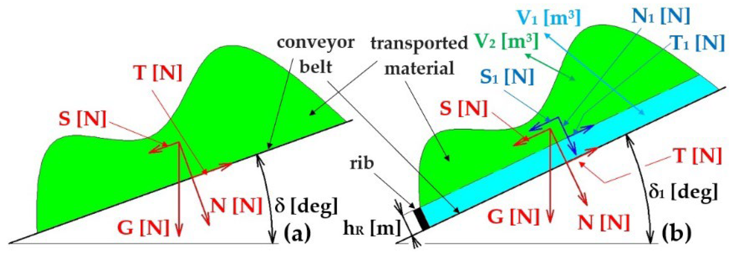
Figure 2.
Cross section of the conveyor belt filling at the used loading width (a) b [m], (b) b1 [m].
Figure 2.
Cross section of the conveyor belt filling at the used loading width (a) b [m], (b) b1 [m].
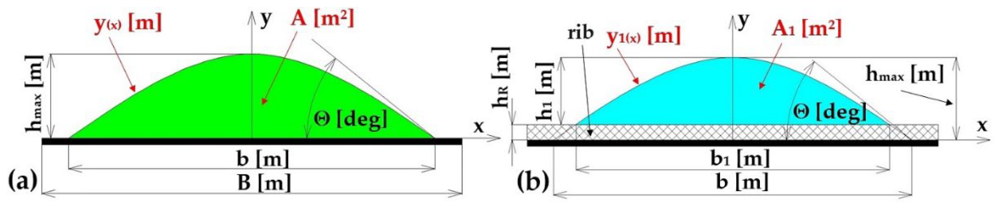
Figure 3.
(a) forces acting on a protrusion inclined at an angle [deg] with respect to the longitudinal axis of the conveyor belt, (b) cross-sectional area A [m2] and volume V [m3] of the conveyed material between the two protrusions, (c) profile conveyor belt [9,10,49].
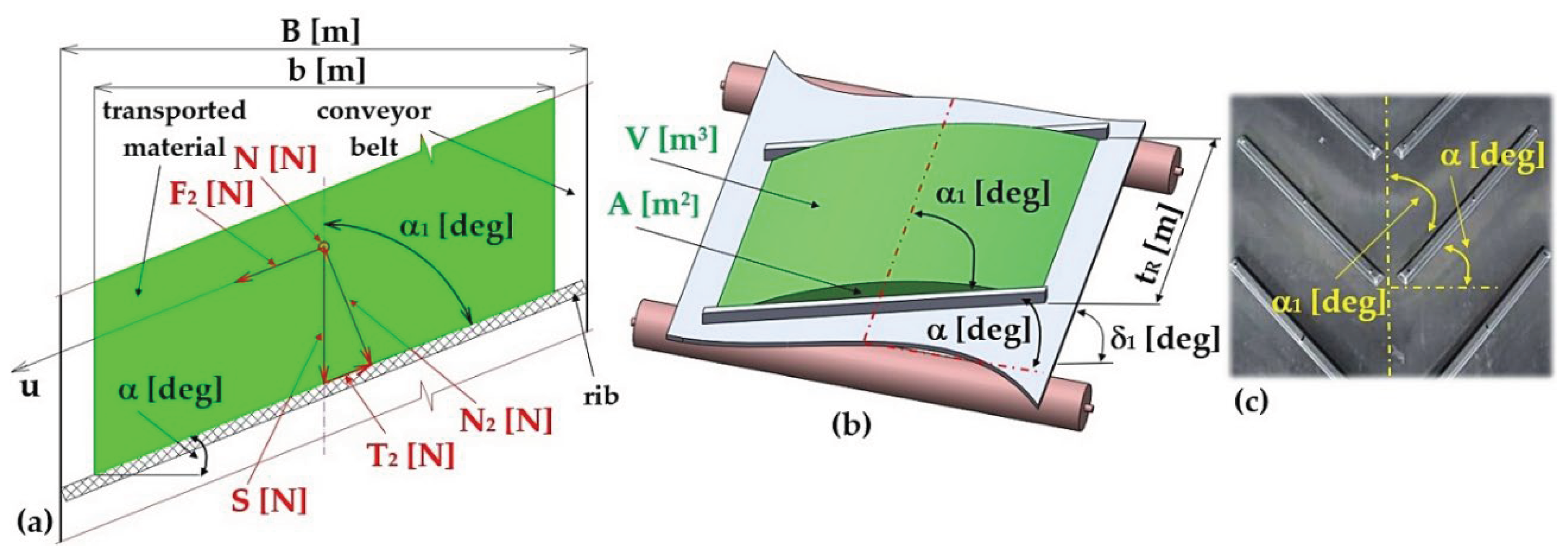
Figure 5.
Structural design of the laboratory device for measuring the compressive force acting on the protrusion (a) 3D model created in SolidWorks 2024, (b) dimensional sketch.
Figure 5.
Structural design of the laboratory device for measuring the compressive force acting on the protrusion (a) 3D model created in SolidWorks 2024, (b) dimensional sketch.
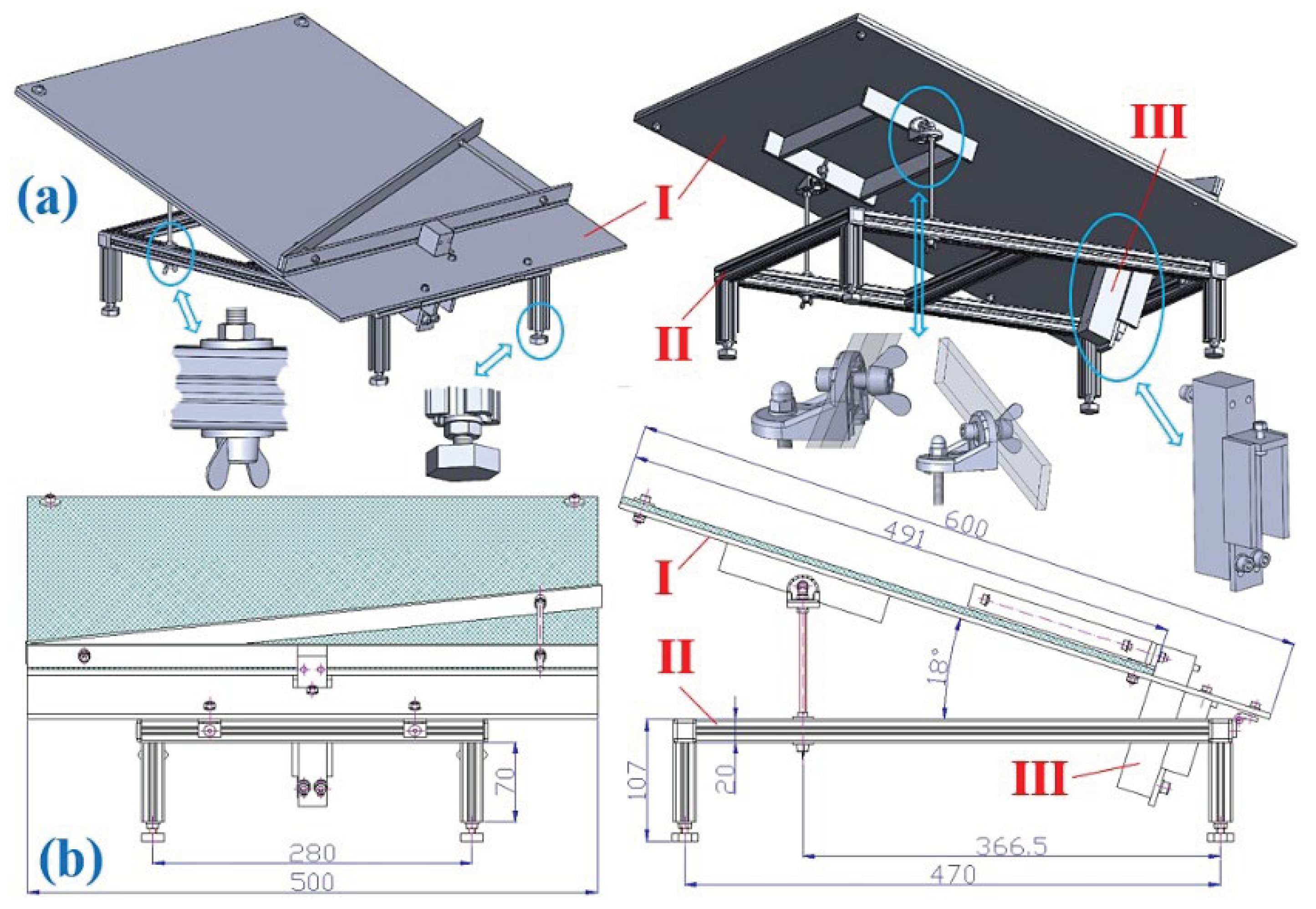
Figure 6.
Measuring chain using DS NET to sense tensile force . 1 – laboratory device, 2 – PLEXI frame, 3 – bulk material, 4 – load sensor [52], 5 – D-Sub plug, 6 – BR4–D measuring module [11], 7 – gateway module DS GATE [53], 8 – network cable, 9 – laptop, 10 – DEWESoft X2 SP5 software [54].
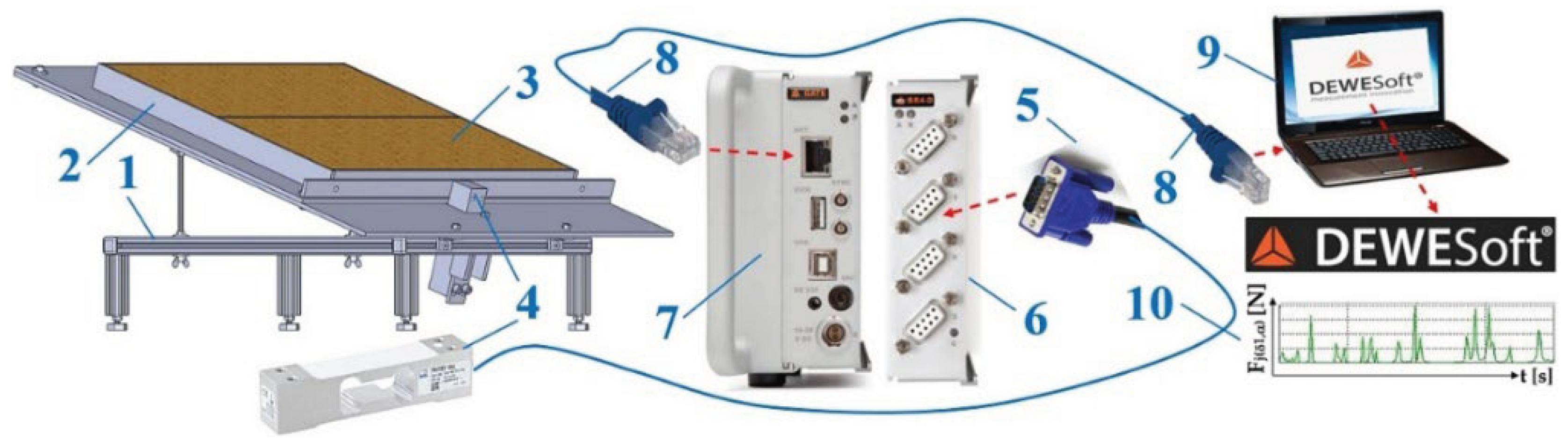
Figure 8.
Measured value of pressure force in the DeweSoft software environment for the angle of protrusion α = 0 deg and the angle of inclination of the conveyor belt = 28 deg.
Figure 8.
Measured value of pressure force in the DeweSoft software environment for the angle of protrusion α = 0 deg and the angle of inclination of the conveyor belt = 28 deg.
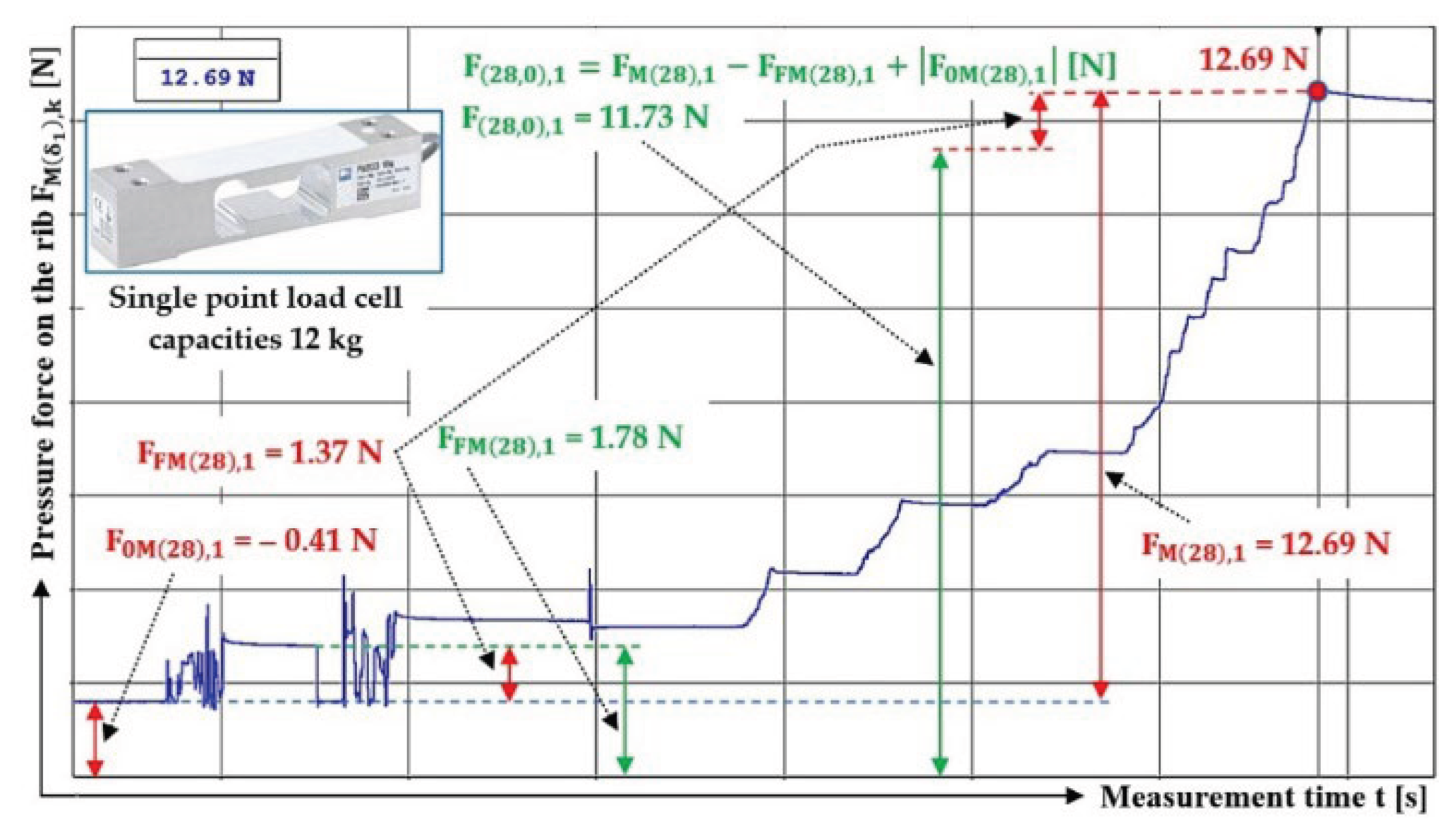
Figure 9.
Measured value of pressure force in the DeweSoft software environment for a protrusion angle of α = 0 deg and a conveyor belt inclination angle of (a) = 32 deg, (b) = 38 deg.
Figure 9.
Measured value of pressure force in the DeweSoft software environment for a protrusion angle of α = 0 deg and a conveyor belt inclination angle of (a) = 32 deg, (b) = 38 deg.
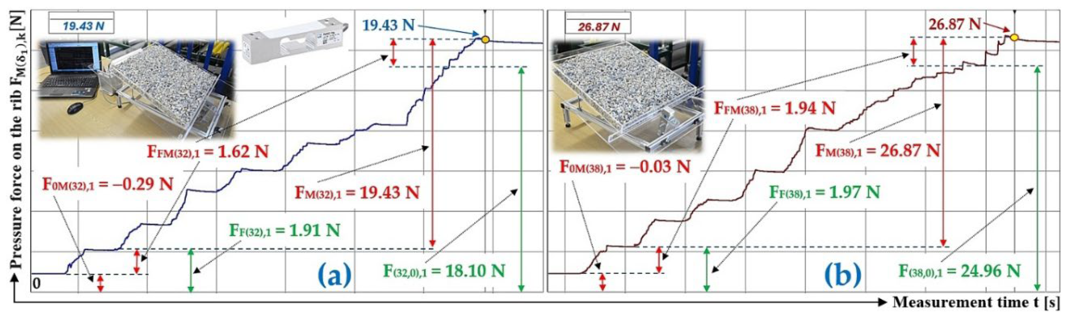
Figure 10.
Measured values in the DeweSoft software environment for α = 15 deg and the angle of inclination of the conveyor belt (a) = 18 deg, (b) = 23 deg.
Figure 10.
Measured values in the DeweSoft software environment for α = 15 deg and the angle of inclination of the conveyor belt (a) = 18 deg, (b) = 23 deg.
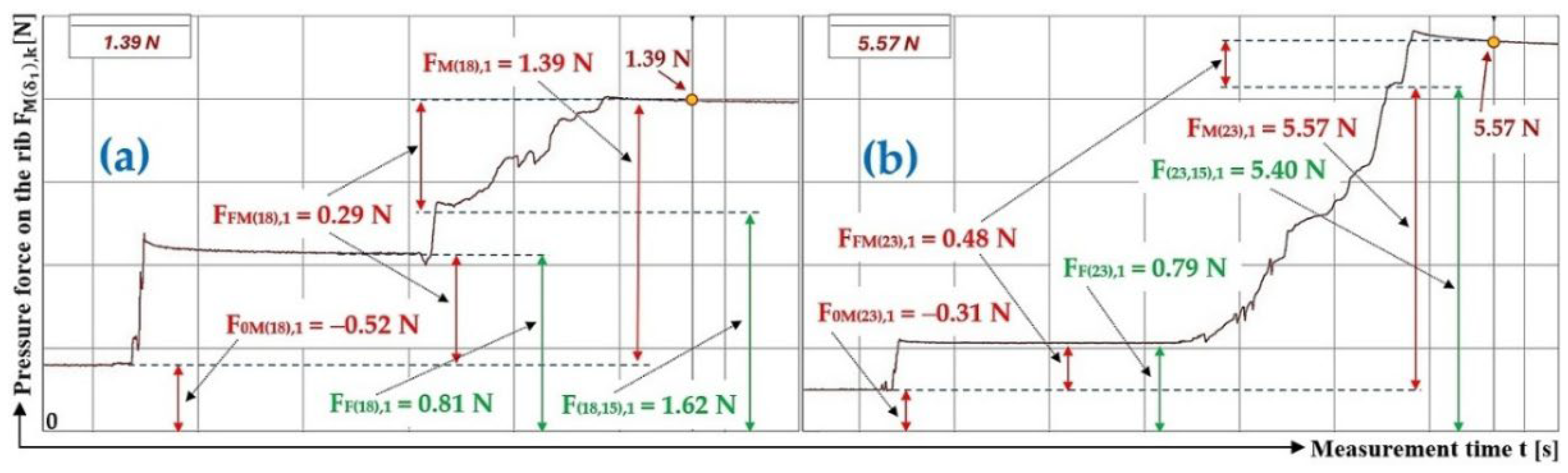
Figure 11.
Measured values in the DeweSoft software environment for α = 15 deg and the angle of inclination of the conveyor belt (a) = 28 deg, (b) = 32 deg.
Figure 11.
Measured values in the DeweSoft software environment for α = 15 deg and the angle of inclination of the conveyor belt (a) = 28 deg, (b) = 32 deg.
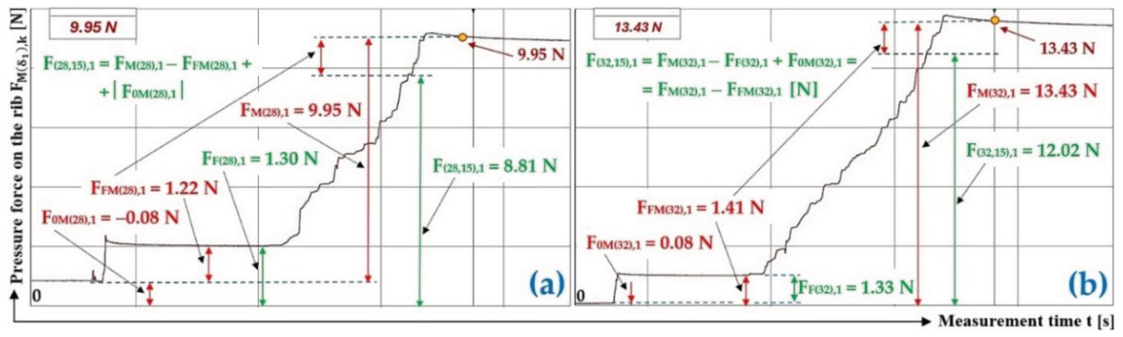
Figure 12.
Measured values in the DeweSoft software environment for α = 15 deg and the angle of inclination of the conveyor belt = 38 deg.
Figure 12.
Measured values in the DeweSoft software environment for α = 15 deg and the angle of inclination of the conveyor belt = 38 deg.
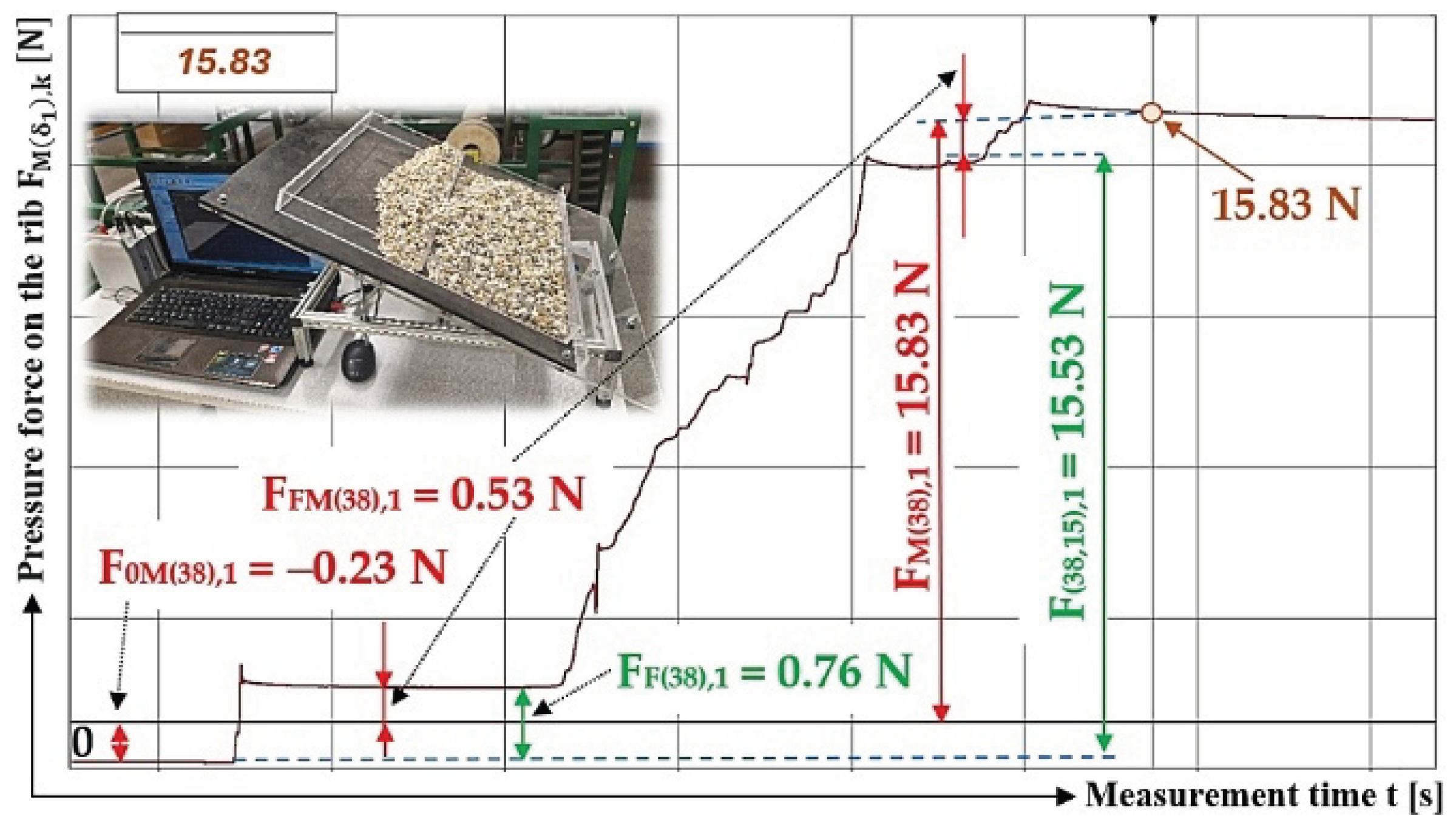
Figure 13.
Measured values in the DeweSoft software environment for α = 0 deg and the angle of inclination of the conveyor belt (a) = 18 deg, (b) = 23 deg.
Figure 13.
Measured values in the DeweSoft software environment for α = 0 deg and the angle of inclination of the conveyor belt (a) = 18 deg, (b) = 23 deg.
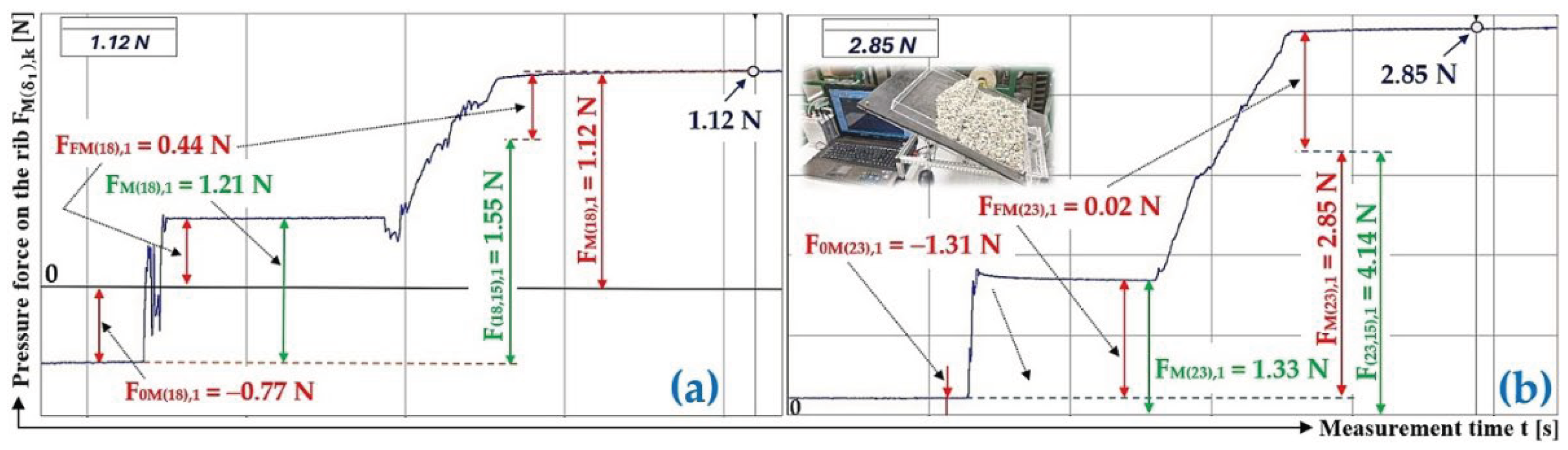
Figure 14.
Measured values in the DeweSoft software environment for α = 0 deg and the angle of inclination of the conveyor belt (a) = 28 deg, (b) = 32deg.
Figure 14.
Measured values in the DeweSoft software environment for α = 0 deg and the angle of inclination of the conveyor belt (a) = 28 deg, (b) = 32deg.
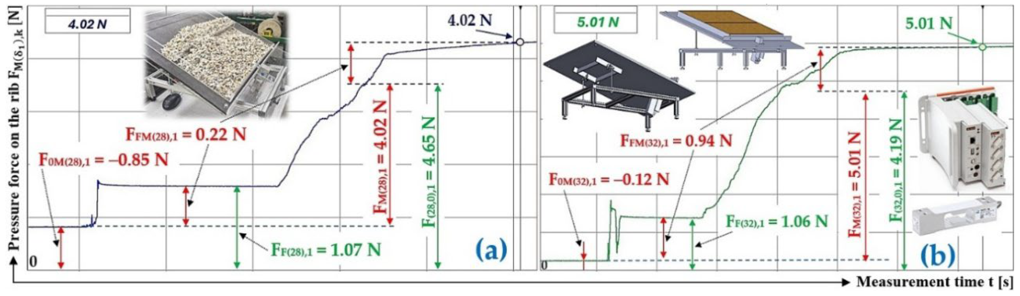
Figure 15.
Measured values in the DeweSoft software environment for α = 0 deg and the angle of inclination of the conveyor belt = 38deg.
Figure 15.
Measured values in the DeweSoft software environment for α = 0 deg and the angle of inclination of the conveyor belt = 38deg.
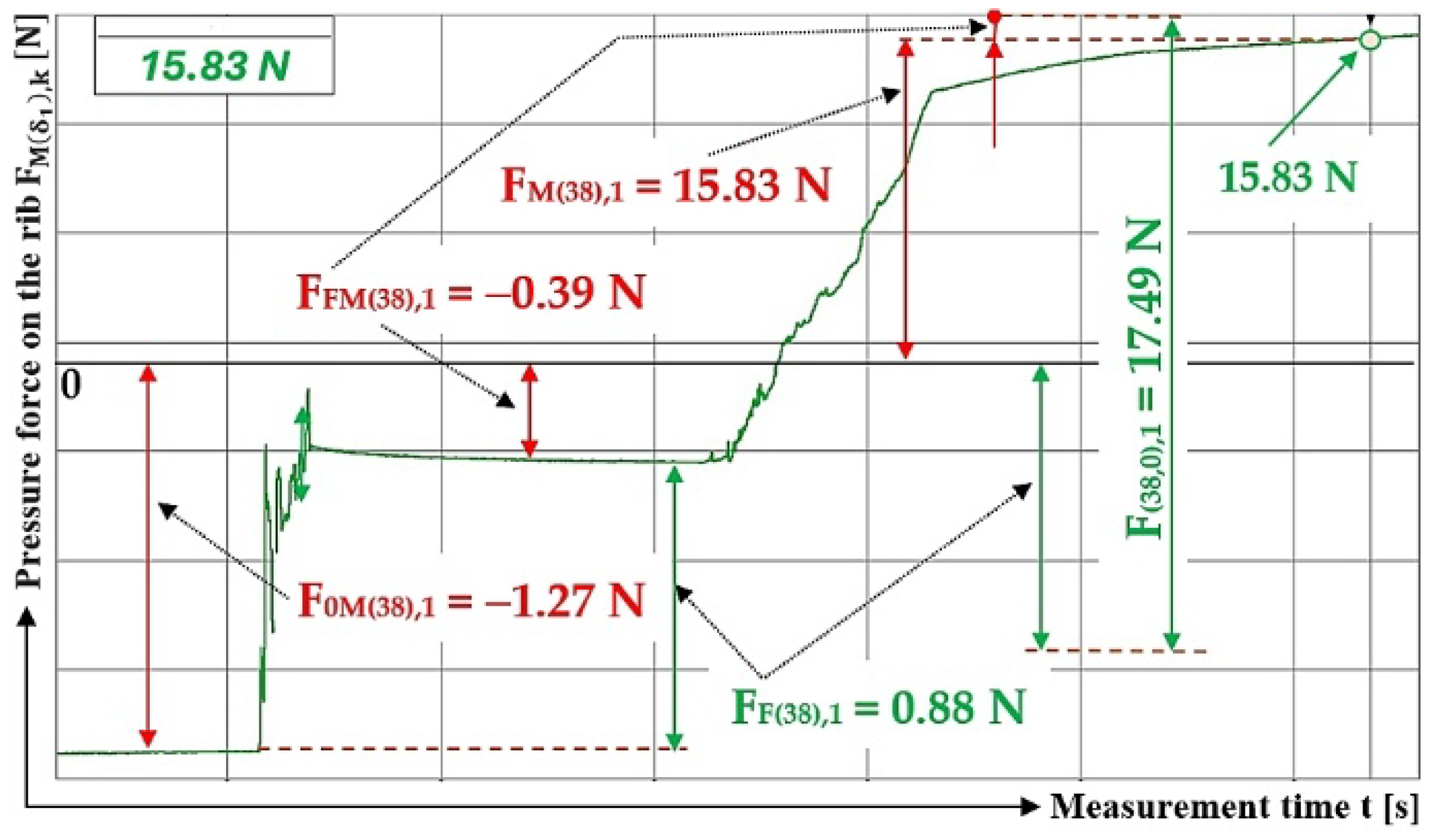
Figure 16.
Measured values in the DeweSoft software environment for α = 15 deg and the angle of inclination of the conveyor belt (a) = 23 deg, (b) = 28 deg.
Figure 16.
Measured values in the DeweSoft software environment for α = 15 deg and the angle of inclination of the conveyor belt (a) = 23 deg, (b) = 28 deg.
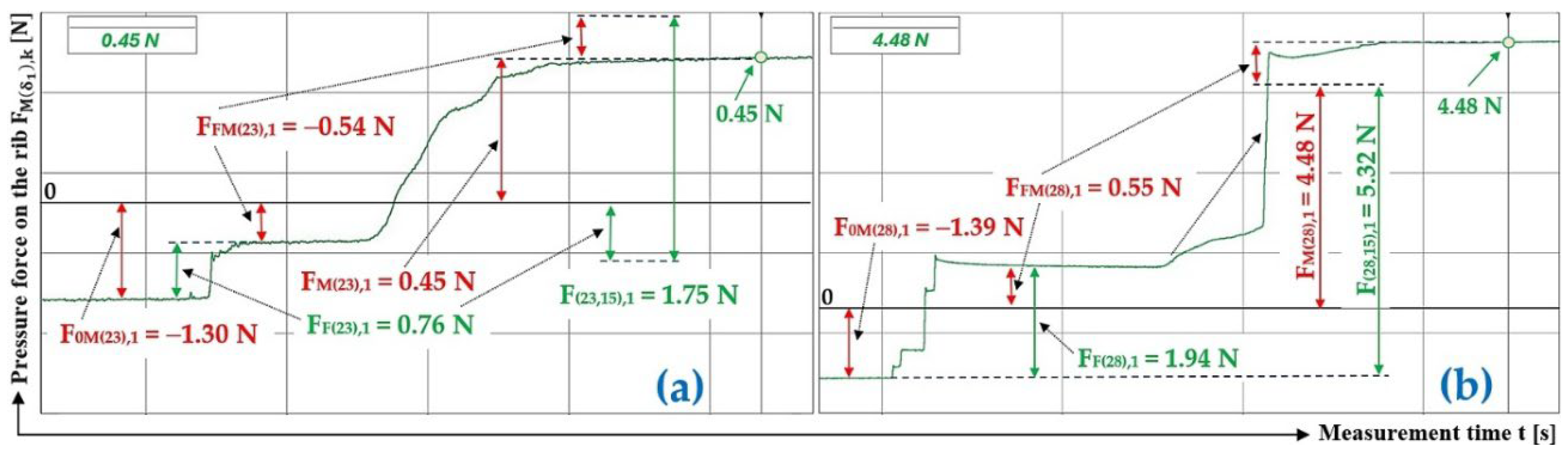
Figure 17.
Measured values in the DeweSoft software environment for α = 15 deg and the angle of inclination of the conveyor belt (a) = 32 deg, (b) = 38 deg.
Figure 17.
Measured values in the DeweSoft software environment for α = 15 deg and the angle of inclination of the conveyor belt (a) = 32 deg, (b) = 38 deg.
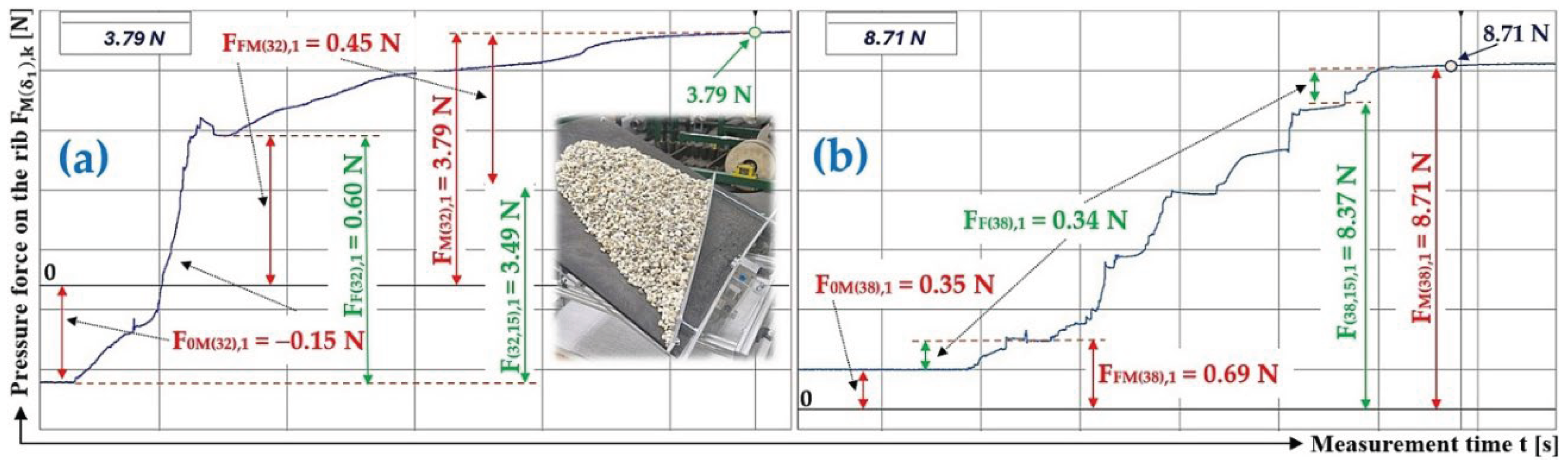
Figure 18.
Values of shear friction coefficient of bulk material (river gravel of 4÷8 mm grain size) in the contact area of the folding plate, inclined at an angle [deg].
Figure 18.
Values of shear friction coefficient of bulk material (river gravel of 4÷8 mm grain size) in the contact area of the folding plate, inclined at an angle [deg].
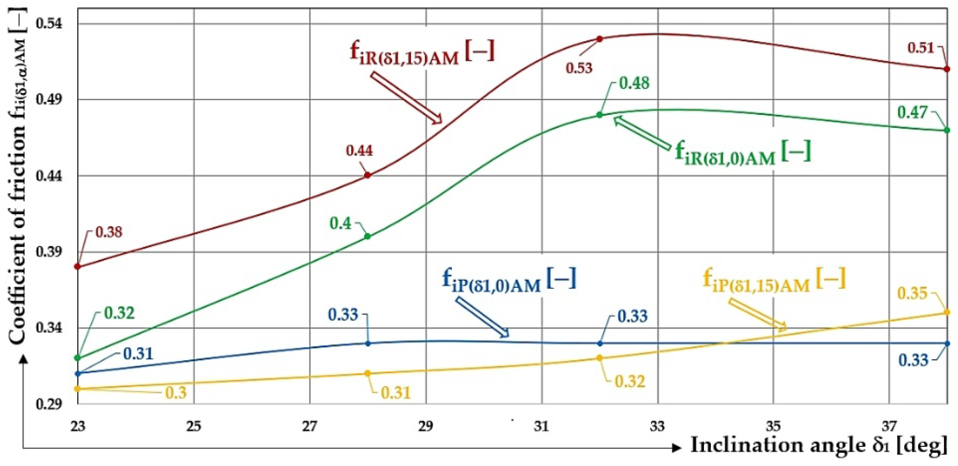
Figure 19.
Measurement of the inclination angle [deg] (a) applied forces during the inclination change of the folding plate, (b) realized measurement. 1 – lower frame, 2 – upper frame.
Figure 19.
Measurement of the inclination angle [deg] (a) applied forces during the inclination change of the folding plate, (b) realized measurement. 1 – lower frame, 2 – upper frame.
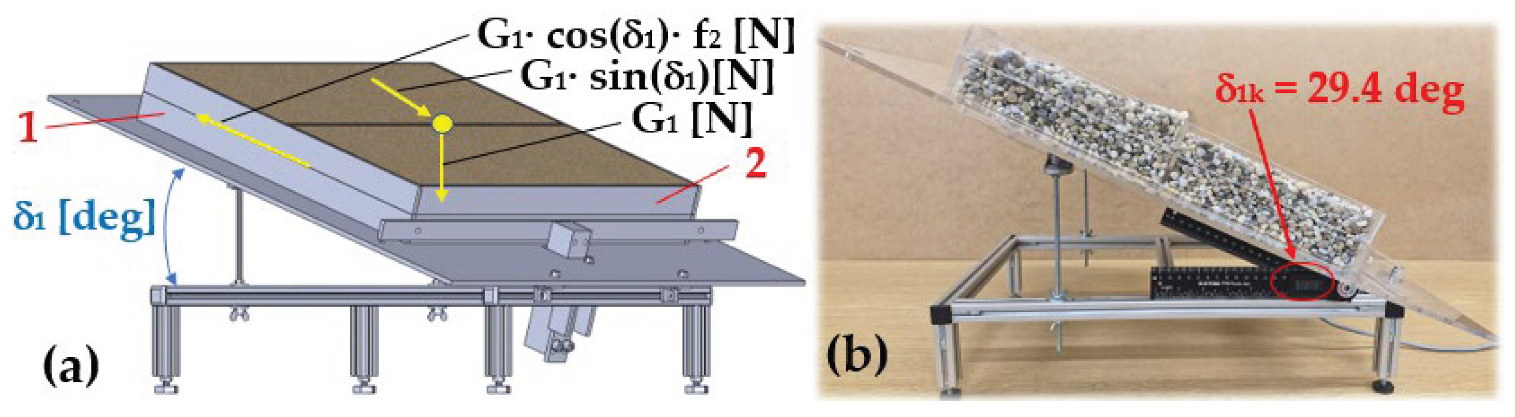
Table 4.
Measured values , , at transport inclination angle = 18 deg and 23 deg and protrusion inclination angle α = 0 deg.
Table 4.
Measured values , , at transport inclination angle = 18 deg and 23 deg and protrusion inclination angle α = 0 deg.
| δ1 | [deg] | 28 | 32 | ||||||||||
|---|---|---|---|---|---|---|---|---|---|---|---|---|---|
| k | G | F0M(28),k | FFM(28),k | FF(28),k | FM(28),k | F(28,0),k | f1P(28,0),k | F0M(32),k | FFM(32),k | FF(32),k | FM(32),k | F(32,0),k | f1P(32,0),k |
| [N] | [N] | [N] | [N] | [N] | [N] | [–] | [N] | [N] | [N] | [N] | [N] | [–] | |
| 1 | 70 | −0.411 | 1.371 | 1.781 | 12.691 | 11.731 | 0.34 | −0.292 | 1.622 | 1.912 | 19.432 | 18.102 | 0.32 |
| 2 | 70 | −0.39 | 1.61 | 2.00 | 13.91 | 12.69 | 0.33 | −0.40 | 1.71 | 2.11 | 18.81 | 17.50 | 0.33 |
| 3 | 70 | −0.37 | 1.28 | 1.65 | 13.78 | 12.87 | 0.32 | −0.32 | 1.69 | 2.01 | 18.76 | 17.39 | 0.33 |
| f1P(28,0)AM = | 0.33 | f1P(32,0)AM = | 0.33 | ||||||||||
| κ(5%,3)28 = | ± 0.02 | κ(5%,3)32 = | ± 0.01 | ||||||||||
Table 5.
Measured values , , at transport inclination angle = 38 deg and protrusion inclination angle α = 0 deg.
Table 5.
Measured values , , at transport inclination angle = 38 deg and protrusion inclination angle α = 0 deg.
| δ1 | [deg] | 38 | |||||
|---|---|---|---|---|---|---|---|
| k | F0M(38),k | FFM(38),k | FF(38),k | FM(38),k | F(38,0),k | f1P(38,0),k | |
| [N] | [N] | [N] | [N] | [N] | [N] | [–] | |
| 1 | 70 | −0.031 | 1.941 | 1.971 | 26.871 | 24.961 | 0.33 |
| 2 | 70 | −0.09 | 1.98 | 2.07 | 26.90 | 25.01 | 0.33 |
| 3 | 70 | −0.06 | 1.96 | 2.02 | 26.84 | 24.94 | 0.33 |
| f1P(38,0)AM = | 0.33 | ||||||
| κ(5%,3)38 = | ± 0.00 | ||||||
1 see Figure 9(b).
Table 6.
Measured values , , at transport inclination angle = 18 deg and 23 deg and protrusion inclination angle α = 15 deg.
Table 6.
Measured values , , at transport inclination angle = 18 deg and 23 deg and protrusion inclination angle α = 15 deg.
| δ1 | [deg] | 18 | 23 | ||||||||||
|---|---|---|---|---|---|---|---|---|---|---|---|---|---|
| k | G | F0M(18),k | FFM(18),k | FF(18),k | FM(18),k | F(18,15),k | f1P(18,15),k | F0M(23),k | FFM(23),k | FF(23),k | FM(23),k | F(23,15),k | f1P(23,15),k |
| [N] | [N] | [N] | [N] | [N] | [N] | [–] | [N] | [N] | [N] | [N] | [N] | [–] | |
| 1 | 45 | −0.521 | 0.291 | 0.811 | 1.391 | 1.621 | 0.29 | −0.312 | 0.482 | 0.792 | 5.572 | 5.402 | 0.29 |
| 2 | 45 | −0.52 | 0.14 | 0.66 | 1.66 | 2.04 | 0.28 | −0.26 | 0.61 | 0.87 | 4.95 | 4.60 | 0.31 |
| 3 | 45 | −0.50 | 0.00 | 0.50 | 1.38 | 1.88 | 0.28 | −0.29 | 0.47 | 0.76 | 4.85 | 4.67 | 0.31 |
| f1P(18,15)AM = | 0.28 | f1P(23, 15)AM = | 0.30 | ||||||||||
| κ(5%,3)18 = | ± 0.01 | κ(5%,3)23 = | ± 0.02 | ||||||||||
Table 7.
Measured values , , at transport inclination angle = 28 deg and 32 deg and protrusion inclination angle α = 15 deg.
Table 7.
Measured values , , at transport inclination angle = 28 deg and 32 deg and protrusion inclination angle α = 15 deg.
| δ1 | [deg] | 28 | 32 | ||||||||||
|---|---|---|---|---|---|---|---|---|---|---|---|---|---|
| k | G | F0M(28),k | FFM(28),k | FF(28),k | FM(28),k | F(28,15),k | f1P(28,15),k | F0M(32),k | FFM(32),k | FF(32),k | FM(32),k | F(32,15),k | f1P(32,15),k |
| [N] | [N] | [N] | [N] | [N] | [N] | [–] | [N] | [N] | [N] | [N] | [N] | [–] | |
| 1 | 45 | −0.081 | 1.221 | 1.301 | 9.951 | 8.811 | 0.31 | 0.082 | 1.412 | 1.332 | 13.432 | 12.022 | 0.31 |
| 2 | 45 | −0.08 | 0.77 | 0.85 | 9.49 | 8.80 | 0.31 | 0.11 | 1.74 | 1.63 | 13.41 | 11.67 | 0.32 |
| 3 | 45 | −0.09 | 1.29 | 1.38 | 9.67 | 8.47 | 0.32 | 0.13 | 1.61 | 1.48 | 13.07 | 11.46 | 0.32 |
| f1P(28,15)AM = | 0.31 | f1P(32, 15)AM = | 0.32 | ||||||||||
| κ(5%,3)28 = | ± 0.01 | κ(5%,3)32 = | ± 0.01 | ||||||||||
Table 8.
Measured values , , at transport inclination angle = 38 deg and protrusion inclination angle α = 15 deg.
Table 8.
Measured values , , at transport inclination angle = 38 deg and protrusion inclination angle α = 15 deg.
| δ1 | [deg] | 38 | |||||
|---|---|---|---|---|---|---|---|
| k | F0M(38),k | FFM(38),k | FF(38),k | FM(38),k | F(38,15),k | f1P(38,15),k | |
| [N] | [N] | [N] | [N] | [N] | [N] | [–] | |
| 1 | 45 | −0.23 | 0.53 | 0.76 | 15.83 | 15.53 | 0.34 |
| 2 | 45 | −0.16 | 0.69 | 0.85 | 15.41 | 14.88 | 0.36 |
| 3 | 45 | −0.19 | 0.62 | 0.81 | 15.27 | 14.84 | 0.36 |
| f1P(38,0)AM = | 0.35 | ||||||
| κ(5%,3)38 = | ± 0.02 | ||||||
1 see Figure 12.
Table 9.
Measured values , , at transport inclination angle = 18 deg and 23deg and protrusion inclination angle α = 0 deg.
Table 9.
Measured values , , at transport inclination angle = 18 deg and 23deg and protrusion inclination angle α = 0 deg.
| δ1 | [deg] | 18 | ||||||
|---|---|---|---|---|---|---|---|---|
| k | G | F0M(18),k | FFM(18),k | FF(18),k | FM(18),k | F(18,0),k | f1R(18,0),k | |
| [N] | [N] | [N] | [N] | [N] | [N] | [–] | ||
| 1 | 70 | −0.771 | 0.441 | 1.211 | 1.121 | 1.551 | 0.30 | |
| 2 | 70 | −1.35 | 0.26 | 1.61 | 1.38 | 2.47 | 0.29 | |
| 3 | 70 | −1.61 | 0.13 | 1.74 | 1.32 | 2.80 | 0.28 | |
| f1R(18,0)AM = | 0.29 | |||||||
| κ(5%,3)18 = | ± 0.02 | |||||||
| δ1 | 23 | |||||||
| k | G | F0M(23),k | FFM(23),k | FF(23),k | FM(23),k | F(23,0),k | f1R(23,0),k | |
| [N] | [N] | [N] | [N] | [N] | [N] | [–] | ||
| 1 | 41 | −1.312 | 0.022 | 1.332 | 2.852 | 4.142 | 0.31 | |
| 2 | 41 | −0.76 | 1.22 | 1.98 | 4.03 | 3.57 | 0.32 | |
| 3 | 41 | −0.60 | 0.48 | 1.08 | 2.97 | 3.09 | 0.34 | |
| f1R(23,0)AM = | 0.32 | |||||||
| κ(5%,3)23 = | ± 0.03 | |||||||
Table 10.
Measured values , , at transport inclination angle = 28 deg and 32 deg and protrusion inclination angle α = 0 deg.
Table 10.
Measured values , , at transport inclination angle = 28 deg and 32 deg and protrusion inclination angle α = 0 deg.
| δ1 | [deg] | 28 | 32 | ||||||||||
|---|---|---|---|---|---|---|---|---|---|---|---|---|---|
| k | G | F0M(28),k | FFM(28),k | FF(28),k | FM(28),k | F(28,0),k | f1R(28,0),k | F0M(32),k | FFM(32),k | FF(32),k | FM(32),k | F(32,0),k | f1R(32,0),k |
| [N] | [N] | [N] | [N] | [N] | [N] | [–] | [N] | [N] | [N] | [N] | [N] | [–] | |
| 1 | 41 | −0.851 | 0.221 | 1.071 | 4.021 | 4.651 | 0.40 | −0.122 | 0.942 | 1.062 | 5.012 | 4.192 | 0.50 |
| 2 | 41 | −1.26 | 0.04 | 1.30 | 4.11 | 5.33 | 0.38 | −0.43 | 1.32 | 1.75 | 5.75 | 4.86 | 0.49 |
| 3 | 41 | −0.58 | 0.76 | 1.34 | 4.75 | 4.57 | 0.41 | −0.15 | 0.53 | 0.68 | 5.96 | 5.58 | 0.46 |
| f1R(18,0)AM = | 0.40 | f1R(23,0)AM = | 0.48 | ||||||||||
| κ(5%,3)28 = | ± 0.03 | κ(5%,3)32 = | ± 0.04 | ||||||||||
Table 11.
Measured values , , at transport inclination angle = 38 deg and protrusion inclination angle α = 0 deg.
Table 11.
Measured values , , at transport inclination angle = 38 deg and protrusion inclination angle α = 0 deg.
| δ1 | [deg] | 38 | |||||
|---|---|---|---|---|---|---|---|
| k | G | F0M(38),k | FFM(38),k | FF(38),k | FM(38),k | F(38,0),k | f1R(38,0),k |
| [N] | [N] | [N] | [N] | [N] | [N] | [–] | |
| 1 | 70 | −1.27 | −0.39 | 0.88 | 15.83 | 17.49 | 0.46 |
| 2 | 70 | −2.83 | −0.56 | 2.27 | 16.64 | 20.03 | 0.47 |
| 3 | 70 | −2.32 | −0.53 | 1.79 | 16.13 | 18.98 | 0.48 |
| f1R(38,0)AM = | 0.47 | ||||||
| κ(5%,3)38 = | ± 0.02 | ||||||
1 see Figure 15.
Table 12.
Measured values , , at transport inclination angle = 23 deg and 28 deg and protrusion inclination angle α = 0 deg.
Table 12.
Measured values , , at transport inclination angle = 23 deg and 28 deg and protrusion inclination angle α = 0 deg.
| δ1 | [deg] | 23 | 28 | ||||||||||
|---|---|---|---|---|---|---|---|---|---|---|---|---|---|
| k | G | F0M(28),k | FFM(23),k | FF(23),k | FM(23),k | F(23,15),k | f1R(23,15),k | F0M(28),k | FFM(28),k | FF(28),k | FM(28),k | F(28,15),k | f1R(28,15),k |
| [N] | [N] | [N] | [N] | [N] | [N] | [–] | [N] | [N] | [N] | [N] | [N] | [–] | |
| 1 | 41 | −1.301 | −0.541 | 0.761 | 0.451 | 1.751 | 0.38 | −1.392 | 0.552 | 1.942 | 4.482 | 5.322 | 0.45 |
| 2 | 41 | −0.43 | −0.14 | 0.29 | 0.77 | 1.20 | 0.39 | −0.16 | 0.28 | 0.44 | 3.15 | 3.03 | 0.45 |
| 3 | 41 | −0.96 | −0.41 | 0.55 | 0.59 | 1.55 | 0.38 | −0.50 | −0.17 | 0.33 | 3.61 | 4.11 | 0.42 |
| f1R(23,15)AM = | 0.38 | f1R(28,15)AM = | 0.44 | ||||||||||
| κ(5%,3)23 = | ± 0.01 | κ(5%,3)28 = | ± 0.03 | ||||||||||
Table 13.
Measured values , , at transport inclination angle = 32 deg and 38 deg and protrusion inclination angle α = 15 deg..
Table 13.
Measured values , , at transport inclination angle = 32 deg and 38 deg and protrusion inclination angle α = 15 deg..
| δ1 | [deg] | 32 | 38 | ||||||||||
|---|---|---|---|---|---|---|---|---|---|---|---|---|---|
| k | G | F0M(32),k | FFM(32),k | FF(32),k | FM(32),k | F(32,0),k | f1R(32,15),k | F0M(38),k | FFM(38),k | FF(38),k | FM(38),k | F(38,0),k | f1R(38,15),k |
| [N] | [N] | [N] | [N] | [N] | [N] | [N] | [N] | [N] | [N] | [N] | [N] | [–] | |
| 1 | 41 | −0.151 | 0.451 | 0.601 | 3.791 | 3.491 | 0.52 | -1.31 | 1.04 | 2.35 | 8.97 | 9.24 | 0.50 |
| 2 | 41 | −0.63 | 1.23 | 1.86 | 3.43 | 2.83 | 0.54 | 0.352 | 0.692 | 0.342 | 8.712 | 8.372 | 0.52 |
| 3 | 41 | −0.71 | 1.16 | 1.87 | 3.38 | 2.93 | 0.54 | -0.21 | 0.13 | 0.34 | 9.04 | 9.12 | 0.50 |
| f1R(32,15)AM = | 0.53 | f1R(38,15)AM = | 0.51 | ||||||||||
| κ(5%,3)32 = | ± 0.02 | κ(5%,3)38 = | ± 0.02 | ||||||||||
Table 14.
Shear friction coefficient of bulk material (river gravel of grain size 4÷8 mm) in the contact surface of the folding plate inclined at an angle [deg].
Table 14.
Shear friction coefficient of bulk material (river gravel of grain size 4÷8 mm) in the contact surface of the folding plate inclined at an angle [deg].
| δ1 [deg] | 18 | 23 | 28 | 32 | 38 | |
|---|---|---|---|---|---|---|
| [−] | 0.28 | 0.311 | 0.331 | 0.331 | 0.331 | |
| 0.28 | 0.302 | 0.312 | 0.322 | 0.352 | ||
| 0.29 | 0.323 | 0.403 | 0.483 | 0.473 | ||
| − | 0.384 | 0.444 | 0.534 | 0.514 | ||
Table 15.
Internal friction angle coefficient (coefficient of shear friction) of bulk material (river gravel of 4÷8 mm grain size) in the contact surface of the folding plate, inclined at an angle [deg].
Table 15.
Internal friction angle coefficient (coefficient of shear friction) of bulk material (river gravel of 4÷8 mm grain size) in the contact surface of the folding plate, inclined at an angle [deg].
| [deg] | 29.41 | 27.6 | 28.1 | 29.2 | 27.9 | |||
| k | 1 | 2 | 3 | 4 | 5 | |||
| [–] | 0.56 | 0.52 | 0.53 | 0.56 | 0.53 | = 0.54 | κ(5%,5) = 0.03 |
1 see Figure 19(b).
Disclaimer/Publisher’s Note: The statements, opinions and data contained in all publications are solely those of the individual author(s) and contributor(s) and not of MDPI and/or the editor(s). MDPI and/or the editor(s) disclaim responsibility for any injury to people or property resulting from any ideas, methods, instructions or products referred to in the content. |
© 2026 by the authors. Licensee MDPI, Basel, Switzerland. This article is an open access article distributed under the terms and conditions of the Creative Commons Attribution (CC BY) license (http://creativecommons.org/licenses/by/4.0/).
Copyright: This open access article is published under a Creative Commons CC BY 4.0 license, which permit the free download, distribution, and reuse, provided that the author and preprint are cited in any reuse.


