
Submitted:
04 January 2026
Posted:
15 January 2026
You are already at the latest version
Abstract
In this paper we derived a novel dynamic dictionary set of algorithms that supports perfectly balanced binary searches for large data sets. The dynamic dictionary is part of our FSP_vgv open source C# package that aims to implement a portable version of Octave/Matlab in order to enable its users to apply the iterative design methodology faster. Our package does not attempt to outdate other software, but fill specialised needs listed in this work. By processing the version control commit history of the FSP_vgv package we validate empirically that with unknown research horizon the time spend developing grows exponentially in the volume of production code. We identify a parameter related to howintuitive a programming language is which also controls the exponential growth of research time hence motivating the need for the highly intuitive Octave/Matlab language and its various software deployments.
Keywords:
dynamic dictionary
; perfectly balanced search
; iterative design
; Octave
; Matlab
; interpreter languages
; open source
1. Introduction
As a method to organize and manage data, dictionaries have been around for thousands of years which makes it one of the oldest known field of research that is still active today [1]. Specifically computer science has been the main driver behind novel dictionary structures due to the sheer number of architectures that require highly customized look up solutions. In essence any function that relies of some data to provide its output needs to perform a search though said data and linear scans that cost are rarely an acceptable option, especially in the age of big data.
The fastest known way to look up data points are hash tables [2] as they offer a constant expected cost of . However hash tables have a number of major disadvantages. First of all there are no universal hash functions [3] meaning that in the worst case a single look up might revert to a linear scan which is worse than a typical binary search that costs . Secondly hash functions typically need to reserve space when initialised and that space will be largely unused for a potentially large number of insert operations. Thirdly, when the hash function is completely full and we want to add more elements we need to initialise a new larger hash table and move everything form the smaller one to the larger one. It is unclear what space we should reserve for the larger hash table and based on the data size and available memory this might be unfeasible.
The classical alternative to hash functions are binary search trees, such as Red-Black Trees [4] and Adelson-Velsky and Landis [5]. Binary searches cost for insert, look up and delete procedures which are slower than hash tables that cost but binary trees do not take extra memory and can typically accept individual dynamic updates that maintain their binary search properties. There are two draw backs of binary trees the first one being that they are more complex to code up and maintain. Secondly and more crucially small tweaks to these algorithms can produce various trade-off between parts of the architecture which can amount to huge gains and loses depending on the problem at hand.
For instance Red-Black trees have a height that is at most meaning that some searches might be twice as fast with a cost of . As a result if we want to look up dictionary elements and then send them over a time sensitive channel the Red-Black tree will incur jitter even before we consider any communication sources of jitter. Alternatively if the binary tree is such that all elements are looked up with a cost of exactly such initial jitter will not be present. In fact, binary searches algorithms where the best and worst case searches are within one step of the best possible are called Perfectly Balanced (PB). As it turns out making sure we can perform perfectly balanced searches often comes at a cost. Therefore there is no one-solution-fits-all dictionary algorithm and we need to find the most suitable dictionary structure to the problem at hand.
Nevertheless, PB trees are highly valued because they are instrumental for latency-sensitive applications, real-time systems and high-performance computing. Therefore, in the highly competitive and hugely oversaturated IT solutions of today even small improvement to PB searches can have huge physical and monetary repercussions [6].
1.1. Related Works
Historically PB searches came at higher maintenance cost. Algorithms such as Day-Stout-Warren [7] can require global rebuilds which is not ideal for highly dynamic scenarios. In addition to that binary trees often ignores cache and memory hierarchy efficiency [8] which further complicates the development of PB searches. As a result we’ve seen the rise of perfectly balanced multi-way trees, such as B-Trees [9] and variants for example, B+ Trees [10,11] which achieve balance but also better the utilization of cache and memory.
One particularly interesting category are Crit-bit Trees [12] [13] that perform a different form of PB searches based on prefixes. The algorithms we proposed in this paper also makes use of prefixes (Sec. 4) but in a very different way due to the fact that we also put the tree within a different framework that utilises tails and additional constructs.
PB searches and dictionaries as concepts also have huge applications in machine learning and robotics. For example the concept of dictionary learning [14,15,16] has become instrumental in the development of large language models. Even if dictionary learning works very differently from a general dictionary in both cases the idea is to learn an empirical basis/set of words from the data which requires structuring the input text for look up.
Importantly dictionaries can be applied not only on text data but also vectorised data for robotics applications as in [17]. Naturally state estimates in robotics are very time-constrained and so balancing the searches is crucial for performance. In the case of [17] the authors maintain performance by automatically re-balancing with partial rebuilds. Similarly in our paper we also set out to perform re-balancing (Sec. 4.3) and we also derive a method that uses two parallel threads for real-time re-building (Sec. 7).
In fact there is so much demand to perform faster look ups such that the dictionary algorithms are put in a larger context of development. For example, in [18] it is suggested that domain experts can benefit from the introduction of higher level, language specific intermediate representation. In the same line of thought some researches for example [19] have also tried to work with functional collections like sets and maps in order to provide better overall performance. These developers also designed their own software package just as we did.
Alternatively some researchers have also attempted to evaluate the actual code of the most commercially valuable applications. For example in [20] the authors look for improvements by comparing and analysing the code of the most well known large language models. However, the models’ code are often not publicly available, leaving many questions about important internal design decisions.
In addition to analysing the code of dictionary algorithms some researchers analyse how to the code developers interact with AI models to build said dictionaries. For example in [21] it was observed that programmers use the AI in two modes: acceleration and exploration. The developers either know what they need and need to get there faster or they are unsure and use the AI to explore options. Knowing about this user pattern the AI can be fine tuned to yield improvements in terms of speed and relevance.
In our paper dictionaries are used in a very unique and relatively uncommon use case. Specifically we developed a novel dictionary that allows an interpreter algorithm to implement a portable instance of Octave/Matlab. The dictionary itself is responsible to insert, delete, look up and copy all variable and results. Our motivation to develop this dictionary and the interpreter stems in essence from the end of Moore’s law [18] and the increased need for [22] Iterative Design (ID) as we discus in more details in Sec 2.1.
Historically one of the most impactful ID’s utility was in rockets science during the Cold War [22] due to the complexity of the problems at hand and the need for quick and viable results. On a higher layer ID is basically equivalent to the scientific method where the difference is that the focus with ID would be on performing more experiments and testing more hypothesis as opposed to spending more efforts on designing better hypothesis.
Even if ID is the de-facto default regime in rocket science such a regime can also arise for simpler cases. Specifically the development of the first commercially viable light bulb by Edison called for the ID approach. In fact some sources unofficially cite Edison as the main inspiration behind Russia’s Cold War rocket program modes of operations and the reason why the Russians managed to be the first to launch various space operations.
Interestingly in this case of the first light bulb the issue was not complexity but the sheer number of possible bulb design and the highly competitive business application. These two domain characteristics cover most of the characteristics of software development as well which suggest that ID is applicable in development of information technologies as shown im [23] and [24]. We further contribute to the utility of ID in IT as discussed in Sec. 2, while we also validate our approach empirically in Sec. 8.
On a broader scale of ID application it is also important to observe that it is also possible to attempt to improve the problem solving of the users though iterative design. For example in [25] the researches apply human centred design in conjunction with ID, while in [26] the researches use ID to produce so called serious games used for education.
Last but not least scientists are aiming to evaluate the human characteristics that drive iterative innovation. For example in [27] by applying cognitive load theory the researchers discovered that when customer heterogeneity rises up to a threshold, the mounting knowledge advantage force promotes the development of iterative innovation.
1.2. Section descriptions
The remainder of this paper is organized as follows. We start with Sec. 2 that gives links to the package repository, commands on how to download and process the difference between commits, explanation for our engineering design choices. Sec. 2.1 gives our ID model that relates the volume of production ready code and the time spend developing it. Sec. 2.2 explains how to install the FSP_vgv package on various devices.
In Sec. 3 we begin defining the FSP_vgv algorithms and structures such as folding, sorting and searches for non dynamic use cases. Then in Sec. 4 we upgrade the algorithms and structures from Sec. 3 to enable dynamic edits in the FSP_vgv and in Sec. 4.4 we prove the computational cost using Cantor’s diagonal principle.
2. Design and Implementation
The proposed set of algorithms that we collectively refer to as the FSP_vgv package [28] is implemented in C# and the latest version can be found in this repository:
The online repository also allows the authors as well as the reader to perform code analysis between version. This is subject matter of Sec. 8 and the git commands to obtain the relevant data is:
git init
git remote add origin https://bitbucket.org/doublevvinged-vladi/fsp_vgv
git remote show origin
git pull origin new_branch
git log --pretty=format:"%H %P" > pair_commits.txt
git diff commit1 commit2 > diff_1_2.txt
The reader might also note that the FSP_vgv package contains an interpreter that can schedule task to the dictionary class FSP_vgv in such a way that the whole package functions as an implementation of the Octave or Matlab software products. This brings us to the objectives of the FSP_vgv product which overlap with the motivation of this paper.
First of all software libraries that run binary searches and are free to use on any operating system are not trivial to find. For example red-black trees are not implemented in the system namespace of C# and therefore any imported library that supports them might also need support across multiple operating systems. The FSP_vgv only import the system namespace of C# and so the package compiles on Windows Linux and on Android though the use of the Termux app.
Secondly online open source libraries often do not contain enough comments, documentation, examples and test procedures that allows a user to maintain them should a mission critical issue arise. Realistically an open source solution should be perceived by its users as a type of hands on manual or tutorial, so that unfamiliar individuals do not have to pay a high effort starter cost even if the solution is provided free of charge. The FSP_vgv is commented and developed in a style similar to Andrew Ng’s Machine Learning course on the coursera.org platform that did its program exercise in Octave. The FSP_vgv has at least one comment for almost any important code line, has build it test function and examples, contains its own documentation and has a function that computes and displays its function definitions.
Next, to simplify the compile command in any command line interface the FSP_vgv is a single text file maintained with the code version features of Bitbucket. As a result even a minimal freely available SDK should be able to compile the package on any OS and on any device simply because there are no external libraries, namespaces and compile settings. This also means that the compiled executable of the package is extremely portable only around 2-3MB compared to Octave and Matlab which are GB in size.
The FSP_vgv is implemented in C# for a number of reason. First of all C# has good memory management features in terms of build in constructor, destructor and garbage collector. Secondly, the syntax is more efficient which allows faster ID. Thirdly C# is large and freely available and many programmes have extensive .NET knowledge. Additionally, C# has various higher level capabilities like multithreading, GPU computing, the ability to take live updates from user inputs as well as ways to perform hardware and network operations.
One important consequence of using C# is that a single class can only be inherited once. Therefore all algorithms related to the dynamic dictionary are within a single class called FSP_vgv and importantly the user is able to do one inheritance on it if needed.
The FSP_vgv interpreter implements the Octave and Matlab language syntax for reason related to ID. Because the modern age has seen rapid developments in big data and machine learning then we’ve seen a degree of standardisation of even more complex solutions like neural networks and dictionary algorithms. As a result the active areas of research and development have entered use cases that are extremely specialised. This implies a paradigm shift.
2.1. Iterative design for niche problems
First of all because the problems at hand are niche and highly specialised then the problem formulations and deliverables will be more vague and the potential results are less likely to be positive. This directly implies that the monetary return is less likely with higher individual milestone risks. In addition to that higher specialization suggests it will be more difficult to find researched able to work on the particular problem due to the amount of domain specific knowledge requirements.
On the other hand, as the IT industry considers more and more edge cases the go-to software like Python, R, MATLAB or Octave in turn will keep running into strange edge cases with respect to either data or implementation specifics. If such a situation arises the researcher will need access and knowledge to the inner-workings of the carrier services, which can only happen if it is open source, relatively small in size to be humanly possible to study within short time frames and extremely comprehensible to avoid mental burn out.
The immediate solution to this paradigm shift is that there will be more need for the ID paradigm to be applied by individual innovators meaning single researches will have to be responsible for the entire tool-chain of their own solution. As we described above the FSP_vgv package aims at allowing individual researcher to apply ID by means of ease of access, lower start up costs, intuitive syntax, comments, etcetera. But we can be more exact in the study of ID for software development.
Assume that there is a volume of code that solves a niche and highly specialised problem for which we have not standard solution, or if it is too elaborate to retro-fit an existing solution to the problem. Let a volume of code x take time T to be coded in a language L giving . Consider then adding lines of code to x resulting in . Consider the meaning of the following derivative in Eq. 1:
From a practical perspective when we use code to search for a solution we make singular attempts to solve the problem at hand (also referred to as iterations) and at the end of the attempt we examine what we’ve learned, redesign, recode and prepare for another attempt. In between attempts it is highly likely that we need to completely delete or edit a large portion of our code since we’ve learned what would not solve the problem and so the derivative in Eq. 1 equals the quantity in Eq. 2
The solution of Eq. 2 is unique and it is the exponential function, meaning
Therefore the single most important parameter to consider in out set up is a code of conduct that reduce the parameter a in Eq. 3. Clearly that parameter is strongly dependent on how intuitive is the programming language. With respect to a R is better than Python because in Python we need to count number of spaces from the beginning of the line to identify clause which slows code edits and increases a. On the other hand Octave is better than R with respect to a because Octave struct arrays don’t need each element to have the same size matrices like in data frames in R. Eq. 3 also explains why we should not use C# directly but utilize the FSP_vgv interpreter as ID speed up.
2.2. Installing on Windows
Dowlonad the free C# SDK. It should be available on all OS, Windows Linux. On Windows locate the csc.exe compliler then open the command line with run this line:
C:\Windows\Microsoft.NET\Framework64\v4.0.30319\csc.exe FSP_vgv_**_t_**.cs
Addapt the command depending on the location of the csc.exe and considering that * represents the current version of the package. The command will produce a FSP_vgv_**_t_**.exe which the user can then run as needed. Simplest possible run command would be:
FSP_vgv_**_t_**.exe user_code.m
which will simply make the interpreter run the user code.
2.3. Installing on Linux or Android
If installing on Android start by installing Termux from the Play Store while it is not needed for Linux. It is important to note that sometimes on Android some files might not be visible and that can be solved by running:
termux-setup-storage
in the command line. This will make a shared folder so that when using the phone in storage mode the user can place his the code in that folder.
Then install Mono by running:
pkg install mono
Next, the FSP_vgv package can be compiled with:
mcs FSP_vgv_**_t_**.cs
which will produce the corresponding executable which can then be run with:
mono FSP_vgv_**_t_**.exe user_code.m
2.4. Differences between the package and its description in this paper
Please note that the package [28] is still under construction so by the time the readers view this paper the package might have changed again. Therefore the main goal of the paper is to convey meaning with clarity and describe the mechanisms and proofs on a higher level and not to overburden with details of secondary importance. As a result the exact way the algorithms of Sec. 3 are implemented in the package [28] are different even if the high level logic is the same. For more information please refer to the build in documentation of [28].
3. Folded Sheet of Paper Elaboration
We start by stating that we are continuing the work done in [29] where binary search was performed on a sorted vector by iteratively relaxing the search interval. The relaxation is performed by comparing the search value with the middle element and then reducing the search interval to the corresponding sub-interval.
Specifically the binary searches in [29] were used for simplicial decomposition and the algorithm appeared first in [30]. Then the binary search was used in [31] for latent variable clustering model and finally to perform search optimization and discrete probability computation in [32]. In essence the binary searches are instrumental in all these cases because we need to perform intersections between sets, meaning we look up n elements of the first set into m elements within the second element and select the common elements to both sets. Without binary searches we perform comparisons while with binary searches we can either run or iterations, which is a huge asymptotic improvement.
To model these binary searches, in the context of object oriented programming and more specifically C# we’ll express the vector as a dynamic list and then we’ll make additional construction on top of the dynamic list to achieve a dynamic dictionary.
We start with notation. We only ever consider a single class and let us call it Folded Sheet of Paper by Vladislav Vasilev (FSP_vgv). We denote each FSP_vgv instance with a capital letter and each attribute of the object with a dot. For example refers to an object with name X and its attribute . Furthermore means that is a pointer of object X currently pointing to Y. When we express then we’ve expressed that there is some pointer of X that points to Y without explicitly stating which one. Therefore a simple dynamic list would look like the example in Figure 1
The intuition behind the algorithms is to consider the dynamic list as a sheet of paper that we recursively fold in half. After n folds we would have split the paper into lines which suggests we can index each line using a binary approach. Because to fold a paper in half all we need is to mark the top, middle and bottom then we’ll express the binary method using pointers from the start to the middle and end of the list. Consider the initial base fold of the list as show in the example in Figure 2.
Let A be the first element of the list. Define two other pointers of the object namely and . Then the initial fold consist of finding that points to the middle of the list in this case D and points to the end of the list in this case G. To compute the middle and end element we can use the initial fold Algorithm 3.
The initial fold Algorithm 3 works by iteratively moving Y from start to end while the middle element X is updated to the next in the list every second increment of the end element Y. Because of this the algorithm costs and it correctly marks the middle and end of the list.
Next for the recursion of the folding consider the example in Figure 4 where we’ve also introduces a pointer to the previous node called .
In Figure 4 the initial fold of Algorithm 3 of the interval halved it into the intervals and . Then we observe that the total in/out degree of each object should be limited sice each class has a fixed number of attributes. This means that when we recur Algorithm 3 on the subintervals we must narrow them so that becomes and becomes . Then we recur Algorithm 3 on the two narrowed subintervals and . We can keep recuring for as long as the two sub intervals has at least 3 elements in them. As a result of Figure 4 we can define the recursive fold Algorithm 5.
Observe that each fold in Algorithm 5 halves the length of the innermost dynamic sublists and that there are at most recursive calls of Algorithm 3 individually costing . Therefore Algorithm 5 costs .
3.1. What is considered a dictionary in the FSP_vgv package
Now that we’ve defined the FSP_vgv folding of a dynamic list we define what it means for a list to be dictionary. To this end let each object X has a field called where is a string of some alphabet. That is to say the names X and Y refer to a particular FSP_vgv object instance while and refers to the string values of each object that we use to compare and order them in the dictionary.
For us to consider a dictionary requires that for two elements X and it also means that that is to say two distinct object must have two distinct names. In short the dictionary only contains unique strings with no duplicates.
Also from a dictionary perspective the strings must be ordered to allow binary look up. To this end we use the alphabet order just as physical dictionary would. Let the alphabet be a string U of length m. If the first character maps to and the first character maps to such that then X should appear in the list before Y. If then we compare the second characters and in the same fashion. If the strings are the same up to a point and then the shorter string should appear first. As a result we can compare two strings to define an order in Algorithm 6.
By Algorithm 6 a dynamic list is considered sorted if for any two consecutive elements X and we also have given the alphabet U. Interestingly if we reorder characters the alphabet U the same set of words would be sorted differently. Now that we’ve defined a dictionary we consider sorting the words in any dynamic list.
3.2. Merge Sorting in the FSP_vgv
Before we can do binary searches in the folded list we need the FSP_vgv to be sorted. This is straight forward to do with merge sort [3] because the FSP_vgv is already partitioned into pairs of lists. Therefore, for the purposes of this subsection assume that the dynamic list was already folded with Algorithm 5 and consider again the example in Figure 4. Furthermore assume that each element now also has a pointer that indicates what is the element that should be in its place in the list after the sorting.
We start by describing the merging of two sorted intervals for the folded FSP_vgv which is given in Algorithm 7. On a high level the smallest element in two sorted lists and is either the first element A of the first list or the first element I of the second list. Hence we can direcly move the smaller element in the output list and move to the next element.
For example if then then incrementing gives the updated interval and as a result the next smallest element after I is either A of or J of .
Alternatively if then then incrementing gives the updated interval and as a result the next smallest element after A is either B of or I of .
As a result merging two sorted lists works by implementing a FIFO type queue between the two lists which requires steps. This logic is described in Algorithm 7.
By utilizing Algorithm 7, we define the entire merge-sort on the folded structure in Algorithm 8. In short the sorting works by selecting the subintervals in each fold then recursively sorting each of them and merging them using Algorithm 7.
Because merging two sorted lists takes and there are at most splits this means the FSP_vgv will be sorted in which is also the same cost of constructing the initial folding. Additionally once we have the sorted values in we must update the , at a cost of and rerun the folding Algorithm 5 with the new dynamic list. Therefore the construction of a sorted and folded FSP_vgv for any input list costs .
3.3. Binary Searches in the FSP_vgv
In this section we assume the FSP_vgv was already sorted and folded then we can perform binary searches with Algorithm 9. The idea behind binary searches in FSP_vgv is straightforward in the sense that we relax the search interval by halving its length on after each set of comparisons. For a given input element we compare it with the current start, middle or end element and either return a missing, recur on the corresponding subinterval or return the exact match.
Because on each recursive call of Algorithm 9 we halve the search interval then there at most calls and that is the cost of the binary search. At this point we also observe that binary searches using Algorithm 9 on structures such as the one in Figure 4 are perfectly balanced because each last node in the binary search takes exactly steps.
4. Dynamic Edits Through Tails and Cantor’s Diagonal Argument
In order to enable dynamic edits in the FSP_vgv we introduce tails for each element in the dynamic list. It is probably interesting to note that this the utilization of tails was inspired by the popular anime characters Naruto and Kurama. When Naruto is threatened he begins morphing gradually into Kurama by iteratively growing more tails of the same length and type until the threat is negated. Similarly each FSP_vgv element now has a pointer that defines its tail and each tail is now separate dynamic list. To distinct the tail list from the original folded and sorted list call non tail elements the main FSP_vgv.
It is very important to note that any tail list is limited to a length of and is not folded or sorted. As a result a binary search to reach a tail takes and then a linear search within that tail also cost to a sum total of to reach a main FSP_vgv element and the search its tail. An example of this is given in Figure 10.
For such a tail construction observe as the data size n becomes large which means that the majority of the data would be in the main FSP_vgv while the tails are relatively short buffer zones. This implies that it is easier for any given tail to get overfilled meaning it would have dynamic elements in it. To avoid this we define a prefix decomposition algorithm.
4.1. Prefix Decomposition
As we defined previously any object X has a single unique string called that we use to place it in the FSP_vgv dictionary and that we use to compare (Algorithm 6) to other elements for sorting and look up. But we can also made the dual argument that the unique entries already in the FSP_vgv dictionary uniquely identify the location of any new object we’d like to place it. This defines a one-to-one relations between any new element and the whole dictionary that is used bellow.
In the context of this section we are not interested in exact match cases in the main FSP_vgv because these elements are edited directly without considering any tail operations. In other words the operations in this section are only meaningful when we look up, insert or delete in the tails.
Start by defining a main prefix for tail operations only. Say we look up in the main FSP_vgv using Algorithm 9 and it returned . The main prefix is a substring of where are all characters from the start of until the last character i are such that . If then the main prefix is . Note if the main prefix is an exact match only when X and Y are exact matches. In short the main prefix is the string that is at the start of both and . The main prefix computation is given Algorithm 11.
Hence observe that the main prefix is precisely the reason why when looking up we find . In order words if we skip the main prefix of and look up the resulting name it will likely not return but a different object for example Z. Computing the main prefix for X and Z will probably give another string that will be different from the original name.
Therefore for any given we can recursively compute its main prefix, then skip the main prefix and recur the main prefix computation. In the process we also compute a set of main FSP_vgv return elements which defines what we’d refer to as a prefix decomposition and this is given in Algorithms 12.
Therefore the main prefix decomposition of Algorithm 12 allows us to use both and the entire dictionary to obtain more than one possible tail where we can fit X. Observe that for names of fixed length q the main prefix decomposition costs and by letting q be constant reverts to . Next we’ll define phantoms elements which are needed in conjunction with the prefix decomposition to enable dynamic edits.
4.2. Phantoms
Recall how in Algorithm 6 we compare and order strings by mapping them to indexes in an alphabet U. In a similar way we can translate any string into a vector using the alphabets, meaning for each i let be and so define . As a result . This defines the one-to-one translation of a string into a vector given an alphabet in Algorithm 13.
Assume we have n elements in the dictionary and that their names have an alphabet U of length m. Define the phantom name length k to be:
, where is the ceiling function. Next for any two elements X and Y in the sorted dictionary such that one follows the other consider their names up to the phantom length meaning and and the vectors and computed using Algorithm 13.
Let and and , then the first phantom node P after X will be such that , that is to say we simply increment to the next character in the alphabet and truncate at the phantom length k. This defines the function . Similarly the phantom Q after P will be such that and we express this as . We stop making phantoms when we reach meaning if . As a result note that adding phantoms to the dictionary costs . Hence we can define how we generate phantoms in Algorithm 14.
To better understand what is the utility of phantom nodes consider the following examples. First of all assume we look up Z in the main FSP_vgv and the binary search returns node X. Furthermore let is the next user node after X that is to say Y is not a phantom. Then we add the appropriate set phantoms between X and Y and return the binary search of Z. Assuming then the binary search will not return X but instead it will return a phantom node in between . Clearly this will reduce the chances of the tail of X to get overfilled, while at the same time the phantom name length k assures that we wont be adding phantoms indefinitely and we’ll take into account the data size n.
Consider a second use case. Consider what happens if we truncate all elements to the phantom length k in a sorted dictionary containing all the phantoms, meaning we run . Because the dictionary is sorted and we’ve filled the space between X and with phantoms then will be all possible words on length k under the dictionary U. Therefore it will not be possible to look up a new and not returning a unique phantom or user element. Therefore we expect the tails to be even less likely to be overfilled given the phantoms.
By these definition phantoms are non-user nodes that are added to the set of main FSP_vgv such that the user can insert in a phantom’s tail while the phantoms will help maintain the dictionary properties. This additional construction will become important when we prove the dictionary edit cost in Sec.4.4.
4.3. Flatten and Rebalance
For the purposes of this section assume we have a sorted and folded FSP_vgv and then by some procedure that is yet to be described but runs a modified prefix decomposition Algorithms 12 we’ve filled all logarithmic tails.
Call the procedure of moving all tail elements of all main dictionary elements back in the set of main FSP_vgv and restoring the dictionary property the flatten and rebalance procedure. This is given in Algorithm 15. Observe that the flatten and rebalancing also adds the phantom nodes.
Observe that the dominating asymptotic cost of the flatten and rebalance Algorithm 15 is determined by the merge sort which yields an overall cost of .
4.4. FSP_vgv Dynamic Dictionary Inspired by Cantor’s Diagonal Principle
Both the prefix decomposition and the phantom nodes were designed to solve the tail overfilling problem however to prove that we can avoid this overfilling entirely we’ll need to re-examine the prefix decomposition.
Observe that for an input Algorithm 12 will partition its name into main prefixes corresponding to the set of dictionary element that are visited by the binary searches. In this set up is the concatenation function of the input string.
Because of the one-to-one mapping then if we permute the name based on the prefixes we’ll create a new name but we’ll visit exactly the same set of elements Q. For example will visit the same but in a permuted order.
As a result if by some chance the user inserts such names that are various main prefix permutations that give the same exact set then these tails will get filled past the logarithmic length while the remaining tails might be completely empty. This will void the dictionary property and to deal with this situation we define permuted names.
Assuming that we’ve inserted phantom nodes in the flatten and rebalance Algorithm Figure 15 which means that for each is a string of length at least . Consider then the string where we concatenate the first character of each main prefix in their respective order. Therefore in general let be a concatenation of the character of each main prefix in the order in which the prefixes appear in the prefix decomposition. Then let us defined the permuted prefix name or more explicitly in Eq. 5:
Next let us run the prefix decomposition on . The first prefixes that appear are guaranteed to be the prefix decomposition of meaning . Following we’ll see a prefix decomposition of the remaining string resulting in . For this prefix decomposition with permuted name we can prove the following theorem:
Theorem 1.
On a FSP_vgv that was flattened and rebalanced using Algorithm 15 performing prefix decomposition with appended permuted names will indicate such tails that any tail will not exceed a length of .
Proof of Theorem 1.
In Table 1 we consider the main prefix decomposition using permuted names according to Eq. 5 of n new elements that we try to insert into a FSP_vgv dictionary that already has n elements in it. Observe how the ordering resembles the proof of Cantor’s diagonal principle.
In Table 1 consider the names and which are different to one another in at least one character. There are two cases. In the first case assume that the main prefixes are unique meaning . In the alternative case we assume for some index mapping between .
- First case, unique prefixes
In the first case implies that the main FSP_vgv elements that we visit are different at least for v meaning and would be inserted in different tails.
- Second case, permuted prefixes
In the second case for some index mapping implies that and might be inserted in the same tails if one of the tails was already full. Therefore consider the sets and . By definition
so substituting gives:
Even is are the same set of string because they are permuted differently and uniquely by the index mapping then and are different. As a result and will be inserted in different tails due to the permuted names.
For a fixed a we’ve proven that any other b will be inserted in a different tail, implies that a will be alone in its tail. Because a is arbitrary then the length of any tail is at most
□
4.5. Non Asymptotic Implications for Theorem 1
It is very important to note that for small data set Theorem 1 will not hold. Specifically for an alphabet of length m and data sets smaller than the main prefix elements will likely have singular characters. This in turn means that the name permute Eq. 5 will not be able to produce a name that is main prefix permutation invariant. Therefore for small data sets it would be easier for the logarithmic tails to get filled and therefore the current version of the FSP_vgv packages checks for tail overfilling and manages is using the flatten and rebalance procedure.
This means that the FSP_vgv algorithms of this work prefer alphabets that are relatively shorter which enable Eq. 5 for smaller data sets and therefore satisfies the conditions of Theorem 1
The current version of the FSP_vgv package actively compares the size of the alphabet and the data sizes to identify if the conditions of Theorem 1 are met and decides based on that if it needs to add phantoms. That is to say phatoms and Theorem 1 are automatically enabled only when the flattern and rebalance procedure encounters a data set that as at least the size of the alphabet squared.
4.6. Algorithms That Work Under the Conditions of Theorem 1
As a result of Theorem 1 we define a new binary search that includes the tails in Algorithm 16.
Next we define a general insert procedure in Algorithm 17. To this end we define a node called which stores at the very least number of edits since the last flatten and rebalance procedure and is such that inserts and deletes do not effect it.
Similarly Algorithm 18 defines the delete procedure under conditions of Theorem 1.
5. Augmenting the FSP_vgv
5.1. Speeding Up FSP_vgv with Nested Dynamic Dictionaries for Latency Sensitive Applications
As we can see in Algorithm 17 and Algorithm 18 if n edits that individually cost to a total of were already performed then we run the flatten and rebalance procedure which costs . Due to Theorem 1 we know for a fact we can insert n elements before we need to rebalance, which means that the average cost per edit that includes the rebalancing is still . Unfortunately this also means that on the edit we’ll have to wait a lot longer for the rebalancing to occur, which is a problem for latency sensitive applications.
Luckily the solution to this problem at least to a degree is made possible by the need of the interpreter to run Matlab’s syntax. More specifically in Matlab when a variable has a dot in its name this means it is a structure containing other structures or variables. To understand why this offers aa solution it’s best to look at an example.
Assume there is a structure variable s containing a variable g representing graph data which would be expressed in Matlab notation as . Next let g be a large graph with vertexes and the vertex data is expressed as a Matlab structure array v for example . Also let s contain a pre-trained neural network model such that is needed for some latency sensitive estimation. Consider in the first case that we allow no nested structures. Then all and will be placed in the same main FSP_vgv as showed in Figure 19.
This means that the edits to will eventually trigger a flatten and rebalancing of the whole main FSP_vgv which also contains and so the latensy sensitive application will have to take into account .
On the other hand if we allow the dot symbol to represent nested dictionaries then edits to can be done while will be accessible though s even if is being rebalanced. An example of this is given in Figure 20.
Therefore by allowing the dynamic dictionary to be nested we decouple the data by its naming convention and allow more flexibility in terms of access latency. Naturally this does not mean that we’ve avoided the rebalancing cost. However with the nested dictionaries we’ve shown that the rebalancing cost is more strongly related to processing of large dictionaries instead of a cost incurred by the structures themselves. This is true because with the appropriate branching of the nested dictionaries we can make certain that rebalancing procedure is almost non existent. The current version of the FSP_vgv package works with nested structures initiated with the dot symbol.
Alternatively the application would have to maintain a permanent access to so that it does not need to look it up every time it is needed which is a more restricting solution.
One other solution would be to always check the notes if an edit would trigger the flatten procedure and incorporate it into the decision making for the latency sensitive application.
5.2. Structure Cloning
An important consequence of allowing nested structure as in Sec. 5.1 is that we can clone structures without running searches. For example is we want to clone in Figure 20 we can clone directly while in Figure 19 we’ll need to look up all element that contain which means we’ll need to do a linear scan of the entire dictionary.
5.3. Reversible Relations for Validation
Importantly, because each element in the FSP_vgv has a limited in/out degree this allows us to make the relations go both ways which is useful if we want to perform a reverse binary search from an any object to the start of the list. This is indispensable for validation and is used in the implementation. For more information please refer to [28].
5.4. True Delete Versus Marked as Deleted or a Phantom
The reader might observe that there is no practical difference between marking a main FSP_vgv node for example as deleted and a phantom node with the same name. In other works there is no way of telling if was added as a phantom node or if the user added a node in the main FSP_vgv and then deleted it. A simple solution would be to just define a variable per node that indicates if the element is a phantom, cleared or occupied. However this is not currently implemented in the package as it adds a layer of complexity that was currently not needed.
On the other side one feature that would be of interest is performing true deletes of a structure because whenever we deal with structures we expect that they could contain large data sets. Therefore it is important to make sure that a delete of a structure is a true delete while we want to be able to go back and validate that we’ve deleted a structure. At the same time we don’t want to add more fields to the class that indicate if the variables was cleared just to maintain lower complexity.
The current version of the FSP_vgv package solves this problem by allowing a nested structure to be represented with two consecutive nodes. For example would have a node and a second node before we reach the variables of . Meaning that if contains v then it would be pointed to by and not directly. Let’s call the intermediate node @.
In this way if we delete we just release and keep . Because of it if we go back and check on we’ll see it has just and no so it means it was a structure and it was cleared. Alternatively if has both and then then we’d expect to be a structure with more data it in. To express an example of this intermediate node solution we draw an additional construction in Figure 20 to produce Figure 21.
It is expected that such scenarios like in Figure 21 might be needed and yield significant improvement for cases with low memory fidelity for example devices that operate in outer space, in high radiation environments or if the device itself has bad memory sectors.
6. When Are Searches Perfectly Balanced?
For an alphabet of size m and a data size phantoms cannot be used because Eq. 5 cannot generate unique names. In this case searches, inserts and deletes in the main FSP_vgv are perfectly balanced and cost . Inserts searches, inserts and deletes in the tails cost at most where is the character length of the name of the data point we are considering. However we might end up overfilling a single logarithmic tail just after inserts which would trigger a flatten and rebalancing that costs . Therefore the total cost of inserts would be . Hence in the case of the worst case cost per single edit is which is not PB.
Once we have enough data meaning phantoms are added that enable Eq. 5 to work and subsequently the conditions of Theorem 1, then the average cost of search, insert and delete becomes . However in this case phantoms exist in between the user data points in the main FSP_vgv. Based on how we defined phantoms between two separate user elements we might have as much as m phantoms meaning that the data that includes the phantoms now has a size of which yields a cost of . To that degree the main FSP_vgv is still perfectly balanced even if it has a constant additional cost. On the other hand edits to the tail cost and we know for a fact from Theorem 1 we can insert n new elements before we need to flatten and rebalance. Therefore the total cost of n edits is and the cost per single edit is which is again perfectly balanced because it is true for all elements.
7. An Additional Construction That Enables Time Sensitive Applications
Due to Theorem 1 we also know that for larger data sets meaning sets where we can generate the permute names we know that the log tails will contain at most one element. This pattern also enable time sensitive applications to be unaffected by the relatively expensive flatten and rebalance procedure by utilising two separate objects that point to the same data. An example of this is given in Figure 22.
In Figure 22 the main FSP_vgv objects are already folded and ready for binary look up. Each object also has a single tail element in correspondence with the result of Theorem 1. Each main or tail FSP_vgv object X points to a which corresponds to a user variable . Observe that the mapping is maintained throughout any pointer operations and we don’t duplicate the data at any point.
Next in Figure 22 we describe the additional construction indicated with an Asterisk (*). The additional main FSP_vgv and the corresponding singular tail elements mirror the original FSP_vgv structure one-to-one.
The starred elements mirror the original structure elements X all the way until we need to flatten and rebalance the X elements. Therefore observe that while we run a flatten and rebalance procedure on X we can freely use the mirrored FSP_vgv for lookup in parallel. As soon as the rebalancing is done then we need to update the mirrored elements in accordance to the flattened FSP_vgv which can also be done in parallel to the main FSP_vgv operations.
As a result even if the insert that triggers the flattening takes much longer to complete the structure would be available for look ups and deletes in the meantime.
8. Results
Because we’ve used a repository to manage the iterative design we can actually validate Eq. 2 and Eq. 3 for the code of the FSP_vgv package, while the data was obtained as explained in Sec. 2. As a result between all two consecutive versions of the package we know exactly how many lines of code were removed and how many were added as well as the total number of lines.
In reality the volume of edits is much larger. First of all the data does not count lines that were moved. Secondly the data does no count lines edits within a versions. For example we might add 100 lines and remove the same 100 lines within a version to run an experiment and then commit the new changes but the final edit count will not have these 100 lines because we completely undid the change just before the commit. Therefore in reality the code edits are fractal in nature, meaning the number of edits vary depending on the measurement units. For example if we saved commits twice as often the number of edits will probably be more than twice as many.
Next, the data is split in two sets. Roughly the first 200 versions were entirely development of the dictionary algorithms. Versions 200 till 600 correspond to the interpreter as well as improvements to the dictionary. For the exponential fit of Eq. 3 to make sense the version count starts at zero.
In the first set in Figure 23 we produced 20,000 lines of code for 200 versions and since the growth is seemingly linear then we’ve been adding 100 lines per version. In the second set in Figure 24 we produced 30,000 lines of code for 400 versions and since the growth is seemingly linear then we’ve been adding 75 lines per version.
This is a very important change as it points out that as the volume of the package increases it becomes more difficult to design changes that make the code better while keeping in mind there are limited number of hours within a workday. In essence we are forced to make a commit sooner because we have a more complex object to keep in check. This phenomenon also changes the a parameter of Eq. 3 such that the parameter of Figure 23 is twice as high as that of Figure 24. This change is not because the software language is suddenly more efficient at expressing the algorithms but rather because of human limitation. On the plus side in both cases the exponential pattern emerges. Meaning that even if the parameter value is context specific the exponential characteristics is not.
As seen in Figure 23 for 20,000 lines of production code we edited 100,000 lines meaning for each 1 line of product code we’ve written and deleted around 4 lines of version code. Similarly in Figure 24 to produce 30,000 lines of product code we edited 250,000 lines of version edits and so for each 1 line of production code we’ve written and edited around 6 lines.
These statistics would be worse with less intuitive language, for example C++. It would be difficult to know exactly how much worse it would be because the current version control was performed with unknown horizon. If we were to recode the algorithms in another language then we’ll be following the specifications of the current FSP_vgv package and the exponential pattern will likely not occur. That is why training developers to code up well established algorithms from scratch is vital as it trains them to make crucial ID decisions for unknown algorithms.
9. Discussion
Before we conclude we can list the strong and weak aspects of the algorithm as well as suggested best use cases. For starters the package is not intended to be used to solve well researched problem for which there is an abundance of online solutions. For example if the user wants to obtain a random sample with a particular distribution it would be best to use the build in functions of R, Mablab, Octave or Python or similar. Just because these functions have been used by a huge number of people, many of whom also consider best practices that generate pseudo random numbers, then the random sample would be reliable and scalable. On the other hand the FSP_vgv does not even implement such functionalities as it is not in its mission objectives.
However if the user is considering a problem that requires ID, meaning large search space, complex object dependencies, distant not well defined research horizon then consider using the FSP_vgv. For example assume we have a large telco data file that is 100GB big and contains 100 KPI columns each of which was enabled at different time during the data collection period. This is not a file that can be loaded in a typical RAM machine while the physical nature of the KPIs means that the way we partition the file must consider radio access arguments. For instance a given KPI could be missing because we have not started collecting it yet or maybe the particular base station was turned off for inspection. Furthermore each telco turns on and off certain KPI depending on needs and availability so the sheer number of KPI combinations would be which is astronomical and the same solution for one telco would likely not work for another telco. That is to say each telco must customise its solutions based on the KPI they decide to enable due the unique engineering challenges they face at different times. In addition to that it is not known in advance what meaningful analysis could be done on the data so the research horizon is not defined.
Next consider a case with structured data or matrices with highly variable sizes. This is common for telco data where each station has its own radio access setup and own set of KPIs. Therefore it would be very common to have a base station be represented with a matrix that has a unique data size that does not repeat across the network. For example a matrix of size 100x20 may never repeat for any other base station out of 9000 in the network. On top of that we may need to sub-select the matrices individually base on behaviours. For example we might want to sub-select rows bases on specific time dependent artefact. Therefore using data frames in R and Python would be very costly as they require all matrices to be of the same size so consider using Octave/Matlab structure arrays or the FSP_vgv package.
In general telco data gives rise to a type of problems with a lot of specifications containing tens of documents each made of hundred of pages just due to the physical nature of the channels. In addition to that some KPIs are very similar and can be collected in different ways. For example a KPI counting hours where the base station was off does not indicate the reason why it was off and it also requires further specification that indicate if outage or power saving is counted as being off. The sheer volume of specification indicate the need for language flexibility and so consider Matlab/Octave and the FSP_vgv package.
Telco data is also typically processed on different operating systems. For example data collection might be done in Linux, but higher level data analytics is visualised on Mac or Windows. In this case the uses might also need to transfer the same exact code solution between operating system ans so consider the FSP_vgv package.
Consider a problem that implies highly limited hard drive space, for example satellite communication or high radiation environments. Even modern day space devices that have to travel outside Earth’s magnetosphere have very limited hard drive [33] simply because radiation causes bit flips. The FSP_vgv package might be a reasonable choice in this case because it is only megabytes in size, has a lot of internal sanity checks and relies on the build in C# memory manager.
The FSP_vgv should also work well in the context of big data where the size of individual matrices or individual strings we consider is much bigger the the memory needed by individual empty FSP_vgv objects. Alternatively if we index individual smaller data objects then the individual FSP_vgv object will take up more memory than the data it represents and that would be less efficient. In the same line of thought if the problem at hand allows at least 8 pointers per object and m empty instances where m is the length of the alphabet then the FSP_vgv package provides applicable data structure.
In some cases the sheer number of dll libraries that are being used in a software solution becomes a problem because libraries begin to require too much support or the number of interfaces that parse data between the packages lead to efficiencies. Because the FSP_vgv package only uses the system namespaces and imports no libraries then it is a viable candidate for this case.
In a more general context some problems require low level access to the carrier software that implements the high level mathematical representations. For example in [34] the authors indicate the use of highly optimized matrix multiplication code. In such scenarios the FSP_vgv can be consider because it give flexible access to how low level operation are performed.
Interestingly there are not many data sources that allow the analysis of the creative process behind software development which to be expected as such analysis can be harmful to the researcher. However, due to the mission critical open source objective of the FSP_vgv package the repository can be used as a realistic instance of how a creative processes unfold as we did in Sec. 8.
Last but not least some problems require a single researches to develop and maintain the entire solution end-to-end and the FSP_vgv package is perfect for this case. For instance in telecommunications in recent years the number of customers has basically stopped growing since everyone already has a mobile device. At the same time the prices of mobile services are expected to drop which means that overall income funds is flattening or decreasing. Therefore new data analytics of telco data will likely have to be done by single innovators. In fact as we are nowadays witnessing the end of Moor’s the entire IT industry will likely encounter the same situation on a daily basis.
10. Conclusions
In this paper we propose a novel dynamic dictionary set of algorithms we implemented in the FSP_vgv package where the user can inset, delete and look up on average with a cost . We’ve proven the asymptotic performance of the algorithms in Theorem 1. As we saw the algorithms rely on a structure that has two parts the the main FSP_vgv and its tails. Due to this characteristic deletes are no true deletes and to mitigate this for structure variables the algorithms also allow sub-dictionaries through the dot sign.
We derived an addition construction that can also enable the package to work with large real-time data and we also explained how sub-dictionaries can also help with time sensitive applications.
We defined the domain of utility for the FSP_vgv package to address problems that require ID, code edit flexibility both on low and high level of coding and abstraction. We’ve analysed the ID approach using the repository’s difference features and concluded that the number of code edits grow exponentially as the production code grows linearly even if the growth parameter is not always constant. This validates the need for solutions such as the FSP_vgv empirically, where we develop with unknown horizons and limited specifications.
Funding
This research was initially only funded by Vladislav Vasilev in the beginning of 2023 and since the start of October 2025 it is also funded by EU project: BG-RRP-2.004-005.
Acknowledgments
The authors acknowledge the significant support of EU project: BG-RRP-2.004-005 including financial, administrative and creative uplift. Spacial thanks go to Cyril Murphy without whom the development of this dynamic dictionary would not have been possible. During the preparation of this study, the authors used OpenAI, Gemini, Copilot and DeepSeek to propose C# code, syntax, namespaces and libraries after being prompted with algorithm specifications by the authors. The same set of AI were also used for literature review. The authors have reviewed and edited the output and take full responsibility for the content of this publication. The FSP_vgv dictionary was entirely created and inveterately re-designed by the Vladislav Vasilev.
Abbreviations
The following abbreviations are used in this manuscript:
| PB | Perfectly Balanced |
| ID | Iterative Design |
| FSP | Folded Sheet of Paper |
| MP | Main Prefix |
References
- Klosa-Kückelhaus, A.; Michaelis, F.; Jackson, H. The design of internet dictionaries. The Bloomsbury Handbook of Lexicography 2022, 1, 405. [Google Scholar]
- Malan, D.J. Hash Tables. Lecture notes for CS50, 2023. Accessed: 2024-01-15.
- Cormen, T.; C. Leiserson, R.R. Introduction To Algorithms; The MIT Press, 2000. [Google Scholar]
- Guibas, L.J.; Sedgewick, R. A dichromatic framework for balanced trees. In Proceedings of the 19th Annual Symposium on Foundations of Computer Science (FOCS)s, 1978; pp. 8–21. [Google Scholar]
- Adelson-Velsky, G.M.; Landis, E.M. An algorithm for the organization of information. Harvard University, 1962, Vol. 146, Proceedings of the USSR Academy of Sciences, pp. 263–266.
- Fischer, M.; Herbst, L.; Kersting, S.; Kühn, L.; Wicke, K. Tree balance indices: a comprehensive survey. arXiv 2021, arXiv:2109.12281. [Google Scholar]
- Stout, Q.F.; Warren, B.L. Tree rebalancing in optimal time and space. 1986, Vol. 29, Communications of the ACM, pp. 902–908.
- Demaine, E.D. Cache-oblivious algorithms and data structures. Lecture Notes from the EEF Summer School on Massive Data Sets, 2002. [Google Scholar]
- Bayer, R.; McCreight, E.M. "Organization and maintenance of large ordered indices,. 1972, Vol. 1, Acta Informatica, p. 173–189.
- Comer, D. The ubiquitous B-tree. 1979, Vol. 11, ACM Computing Surveys (CSUR).
- M. A. Bender, E.D.D.; Farach-Colton, M. Cache-oblivious B-trees. SIAM Journal on Computing 2005, 35, 341–358. [Google Scholar] [CrossRef]
- Bernstein, D.J. Crit-bit trees. http://cr.yp.to/critbit.html, 2004.
- Morrison, D.R. PATRICIA—Practical Algorithm To Retrieve Information Coded in Alphanumeric. Journal of the ACM 1968, 15, 514–534. [Google Scholar] [CrossRef]
- Tariyal, S.; Majumdar, A.; Singh, R.; Vatsa, M. Deep dictionary learning. IEEE Access 2016, 4, 10096–10109. [Google Scholar] [CrossRef]
- Tolooshams, B.; Song, A.; Temereanca, S.; Ba, D. Convolutional dictionary learning based auto-encoders for natural exponential-family distributions. In Proceedings of the International Conference on Machine Learning. PMLR, 2020; pp. 9493–9503. [Google Scholar]
- Zheng, H.; Yong, H.; Zhang, L. Deep convolutional dictionary learning for image denoising. In Proceedings of the Proceedings of the IEEE/CVF conference on computer vision and pattern recognition, 2021; pp. 630–641. [Google Scholar]
- Cai, Y.; Xu, W.; Zhang, F. ikd-tree: An incremental kd tree for robotic applications. arXiv 2021, arXiv:2102.10808. [Google Scholar]
- Lattner, C.; Amini, M.; Bondhugula, U.; Cohen, A.; Davis, A.; Pienaar, J.; Riddle, R.; Shpeisman, T.; Vasilache, N.; Zinenko, O. MLIR: A compiler infrastructure for the end of Moore’s law. arXiv 2020, arXiv:2002.11054. [Google Scholar]
- Dhulipala, L.; Blelloch, G.E.; Gu, Y.; Sun, Y. Pac-trees: Supporting parallel and compressed purely-functional collections. In Proceedings of the Proceedings of the 43rd ACM SIGPLAN International Conference on Programming Language Design and Implementation, 2022; pp. 108–121. [Google Scholar]
- Xu, F.F.; Alon, U.; Neubig, G.; Hellendoorn, V.J. A systematic evaluation of large language models of code. In Proceedings of the Proceedings of the 6th ACM SIGPLAN international symposium on machine programming, 2022; pp. 1–10. [Google Scholar]
- Barke, S.; James, M.B.; Polikarpova, N. Grounded copilot: How programmers interact with code-generating models. Proceedings of the ACM on Programming Languages 2023, 7, 85–111. [Google Scholar] [CrossRef]
- Larman, C.; Basili, V.R. Iterative and incremental developments. a brief history. Computer 2003, 36, 47–56. [Google Scholar] [CrossRef]
- Tsai, B.Y.; Stobart, S.; Parrington, N.; Thompson, B. Iterative design and testing within the software development life cycle. Software Quality Journal 1997, 6, 295–310. [Google Scholar] [CrossRef]
- Gossain, S.; Anderson, B. An iterative-design model for reusable object-oriented software. ACM Sigplan Notices 1990, 25, 12–27. [Google Scholar] [CrossRef]
- Siena, F.L.; Malcolm, R.; Kennea, P.; et al. DEVELOPING IDEATION & ITERATIVE DESIGN SKILLS THROUGH HUMAN-CENTRED PRODUCT DESIGN PROJECTS. In Proceedings of the DS 137: Proceedings of the International Conference on Engineering and Product Design Education (E&PDE 2025), 2025; pp. 595–600. [Google Scholar]
- Viudes-Carbonell, S.J.; Gallego-Durán, F.J.; Llorens-Largo, F.; Molina-Carmona, R. Towards an iterative design for serious games. Sustainability 2021, 13, 3290. [Google Scholar] [CrossRef]
- Jiang, X.; Jin, R.; Gong, M.; Li, M. Are heterogeneous customers always good for iterative innovation? Journal of Business Research 2022, 138, 324–334. [Google Scholar] [CrossRef]
- Vasilev, V. Folded sheet of paper. Bitbucket, 2024. Self-published.
- Vasilev, V. Algorithms and Heuristics for Data Mining in Sensor Networks; LAP LAMBERT Academic Publishing, 2016. [Google Scholar]
- Vasilev, V. Chromatic Polynomial Heuristics for Connectivity Prediction in Wireless Sensor Networks. In Proceedings of the ICEST 2016, Ohrid, Macedonia, 28-30 June 2016. [Google Scholar]
- Vasilev, V.; Iliev, G.; Poulkov, V.; Mihovska, A. A Latent Variable Clustering Method for Wireless Sensor Networks. submitted to the Asilomar Conference on Signals, Systems, and Computers, November 2016. [Google Scholar]
- Vasilev, V.; Leguay, J.; Paris, S.; Maggi, L.; Debbah, M. Predicting QoE factors with machine learning. In Proceedings of the 2018 IEEE International Conference on Communications (ICC). IEEE, 2018; pp. 1–6. [Google Scholar]
- ESA. LEON2 / LEON2-FT. https://www.esa.int. Accessed: 2025-11-24.
- Vaswani, A.; Shazeer, N.; Parmar, N.; Uszkoreit, J.; Jones, L.; Gomez, A.N.; Kaiser, Ł.; Polosukhin, I. Attention is all you need. Advances in neural information processing systems 2017, 30. [Google Scholar]
Figure 1.
Example dynamic list.

Figure 2.
Initial fold of the list.
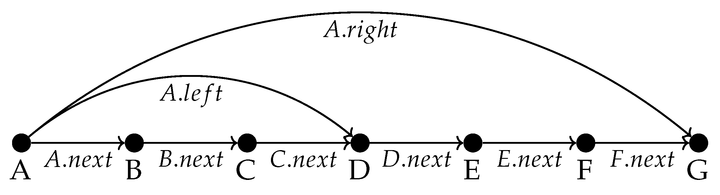
Figure 3.
Initial fold of the dynamic list in Figure 2.
Figure 3.
Initial fold of the dynamic list in Figure 2.
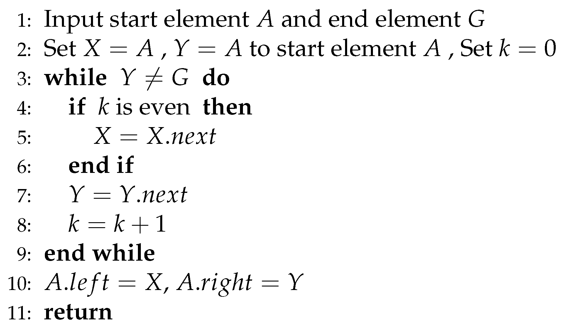
Figure 4.
Recursive fold.
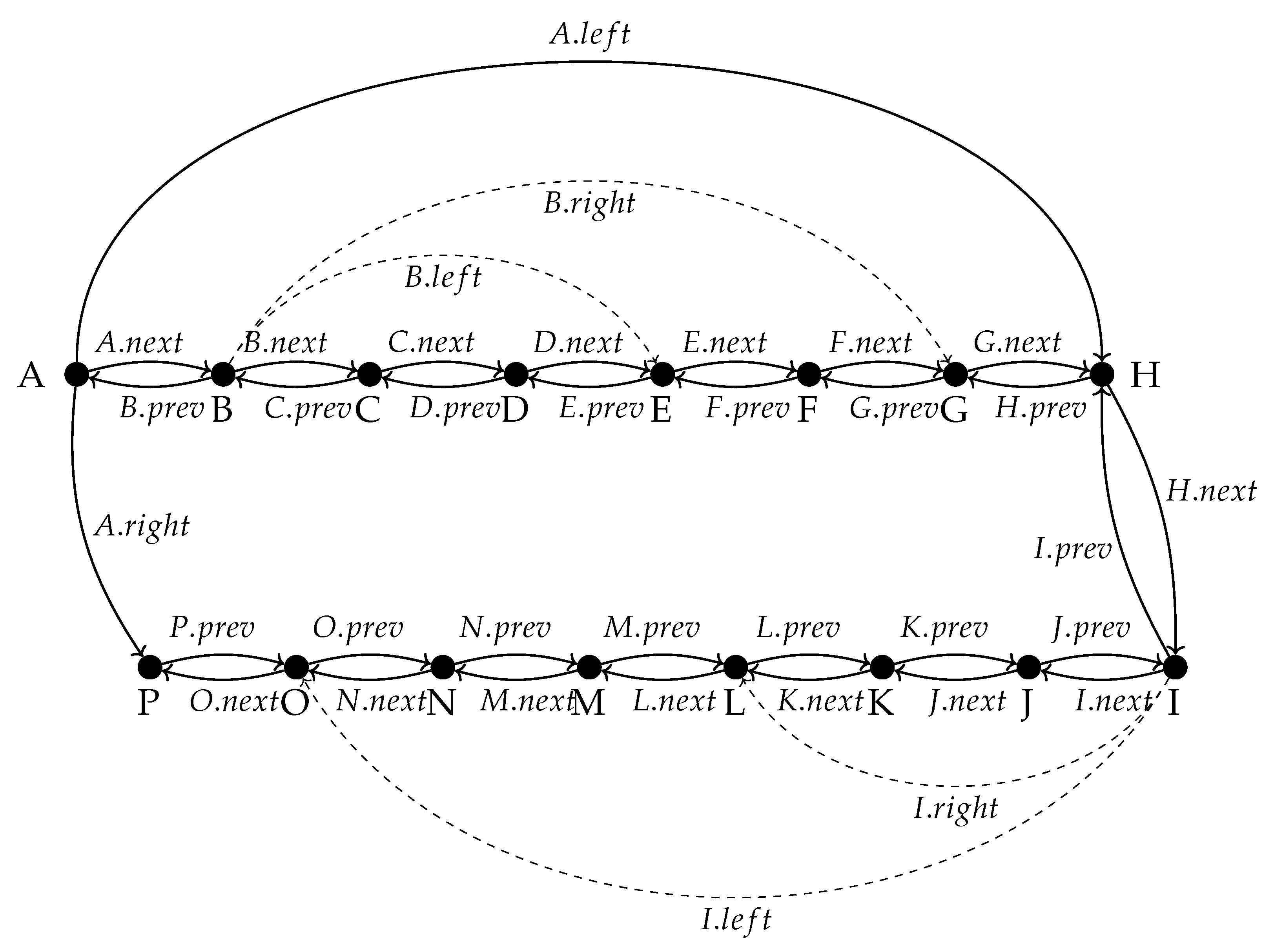
Figure 5.
Recursive fold of the dynamic list in Figure 4.
Figure 5.
Recursive fold of the dynamic list in Figure 4.
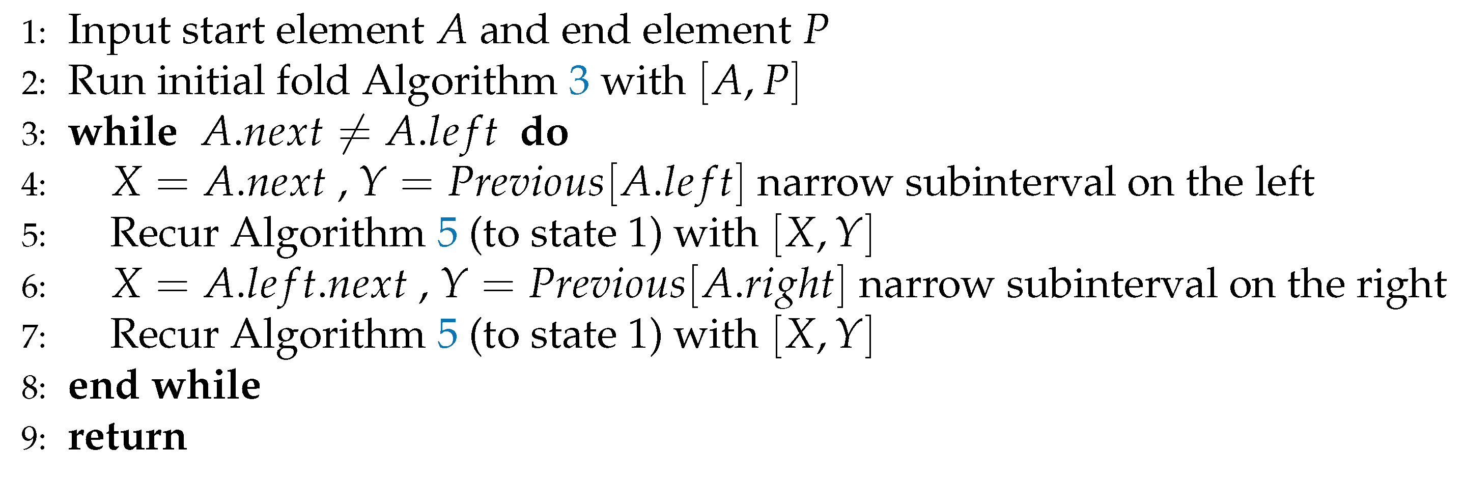
Figure 6.
Compare two strings.
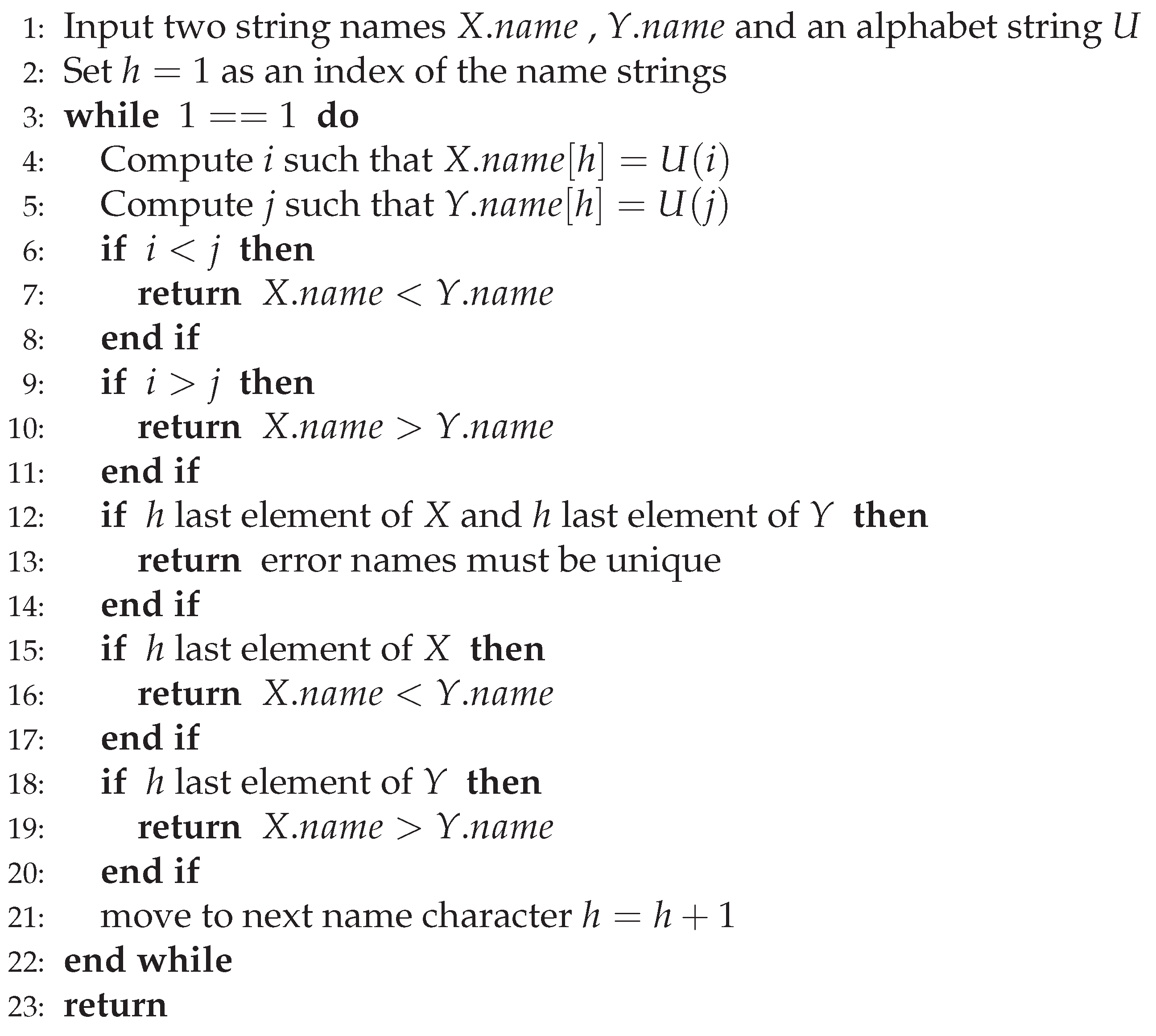
Figure 7.
Merging two sorted intervals in Figure 4.
Figure 7.
Merging two sorted intervals in Figure 4.
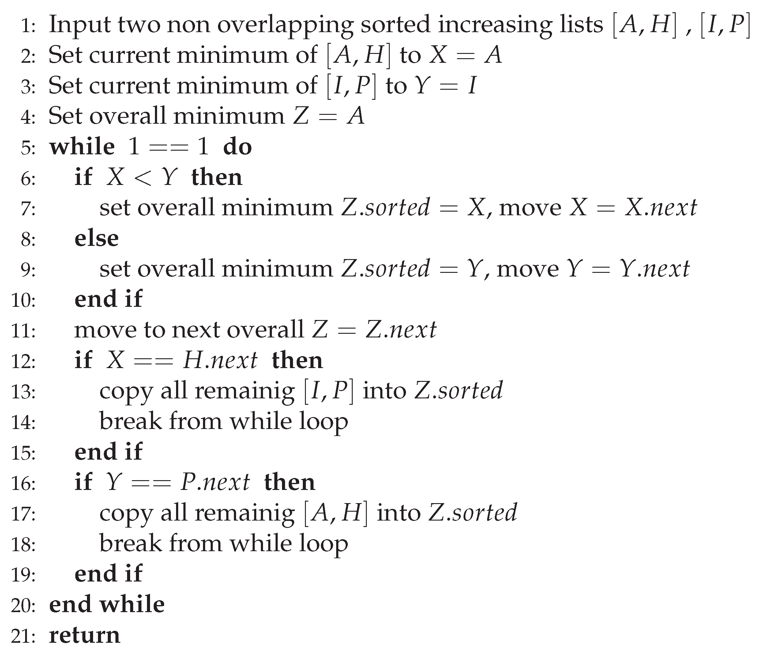
Figure 8.
Merge sort in Figure 4.
Figure 8.
Merge sort in Figure 4.
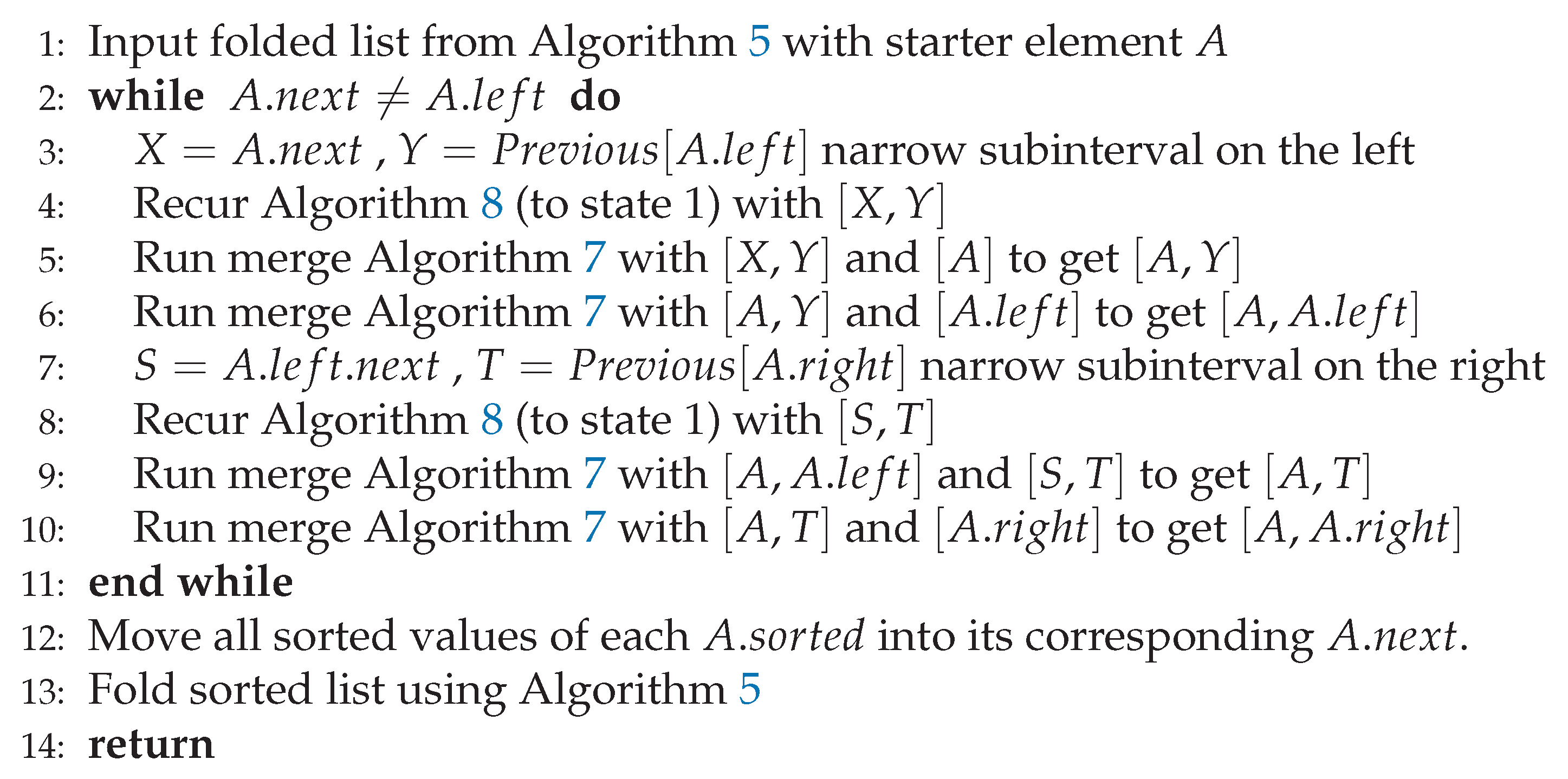
Figure 9.
Binary searching is sorted and folded FSP_vgv list.
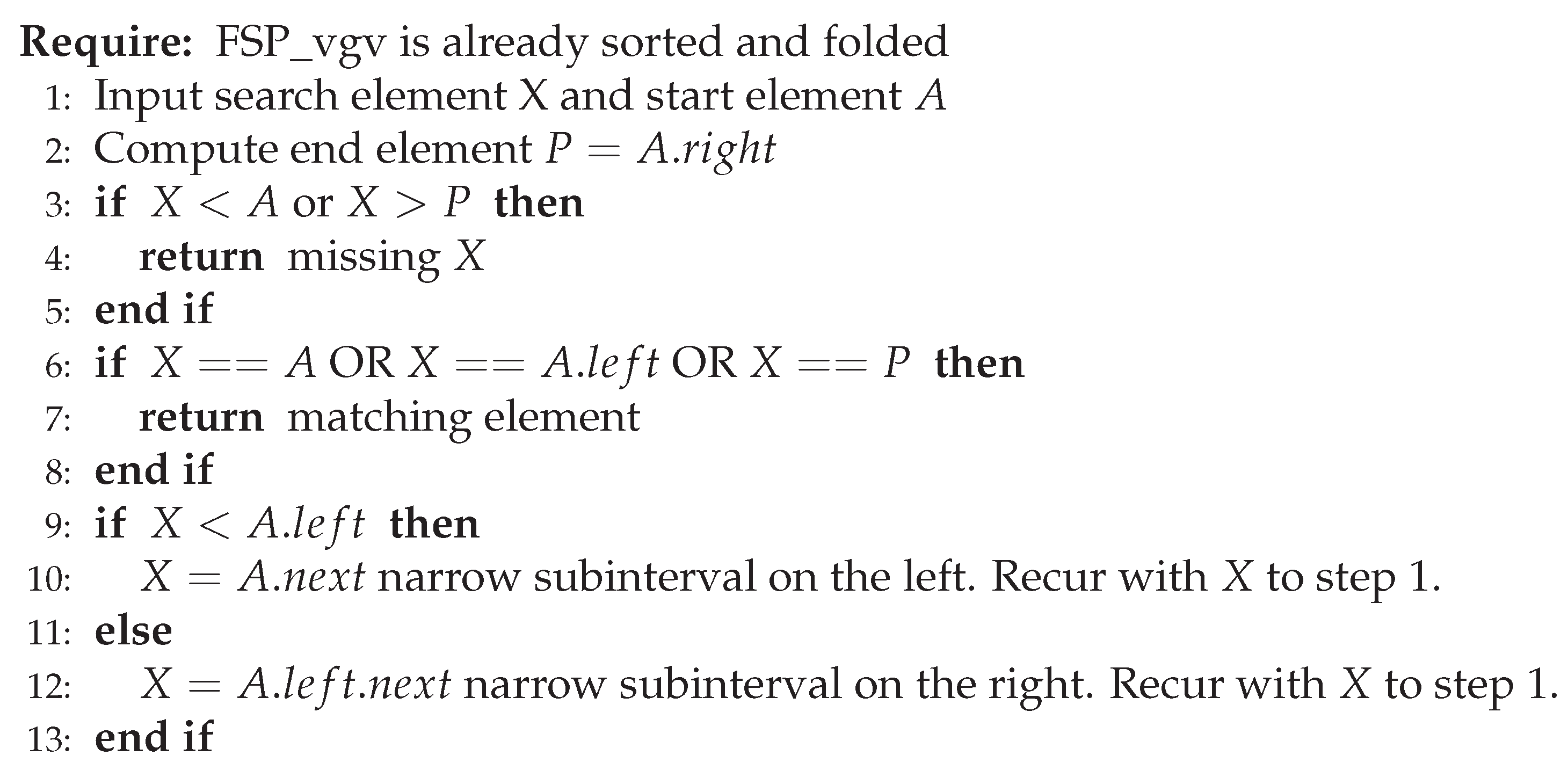
Figure 10.
Logarithmic Tails.
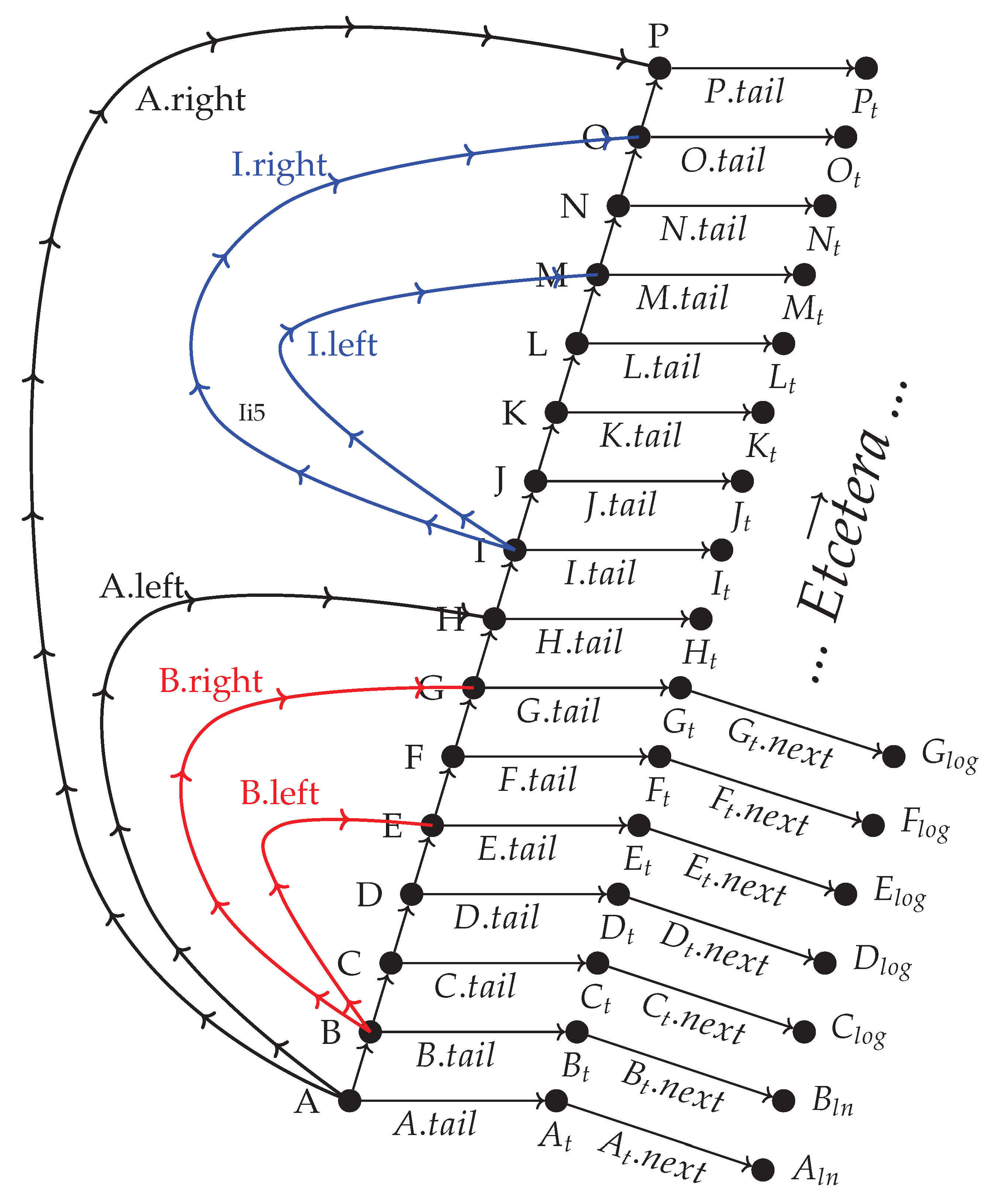
Figure 11.
Main prefix.
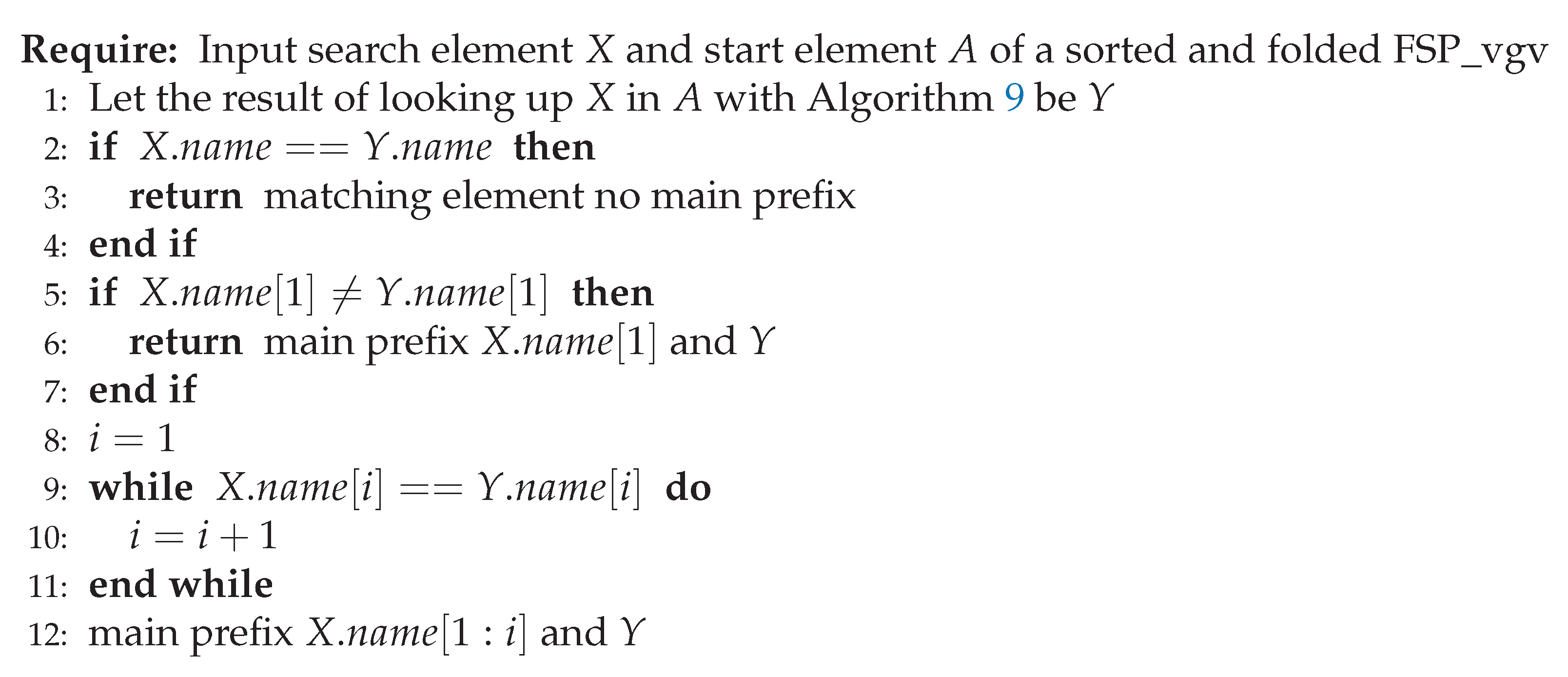
Figure 12.
Prefix recomposition.
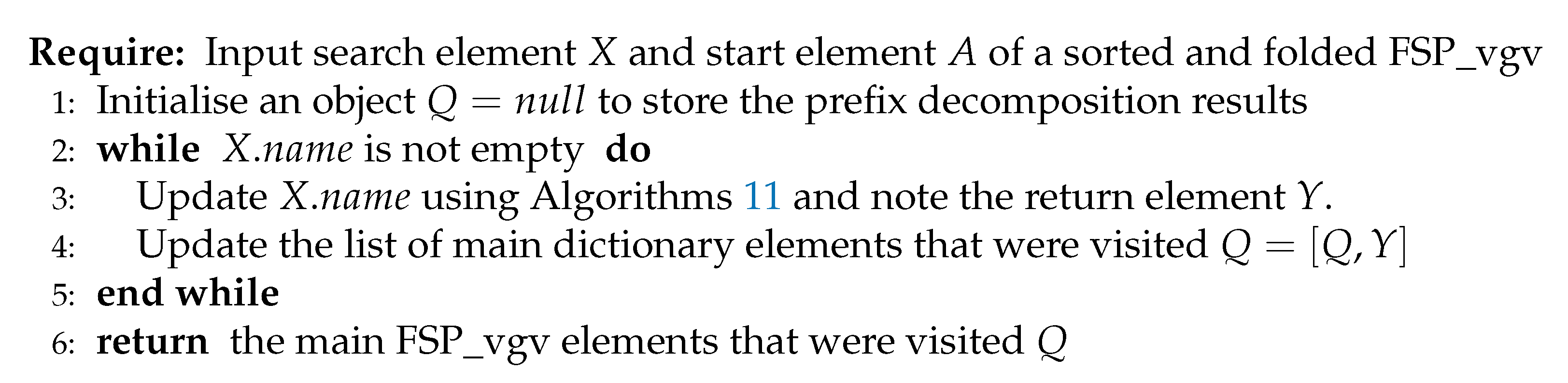
Figure 13.
One-to-one translation of a string into a vector given an alphabet.
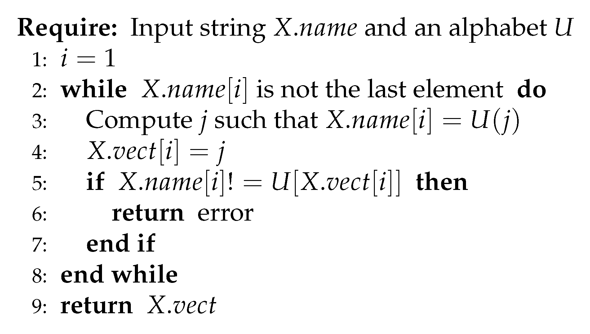
Figure 14.
Generating the phantoms between X and .
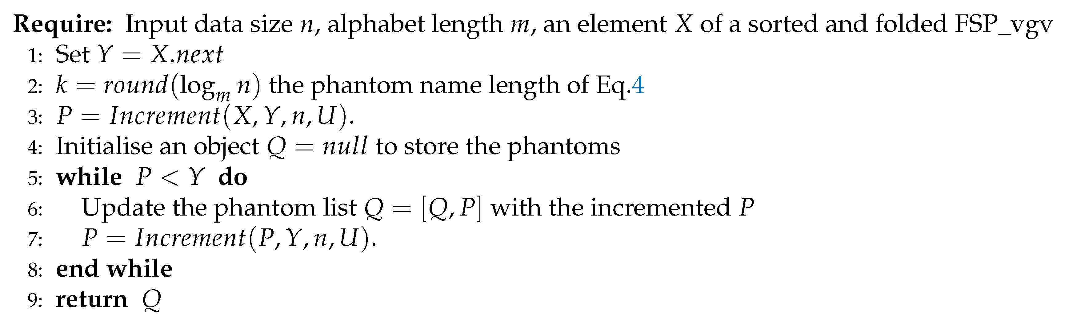
Figure 15.
Flatten and rebalance.
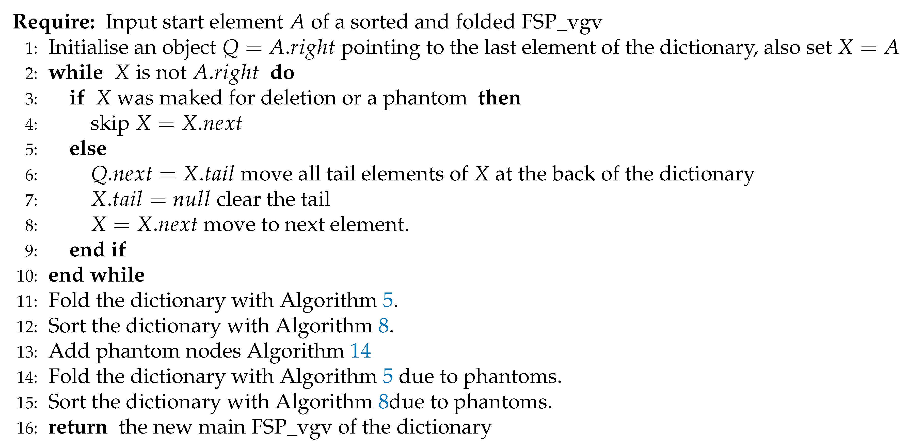
Figure 16.
Revised binary search
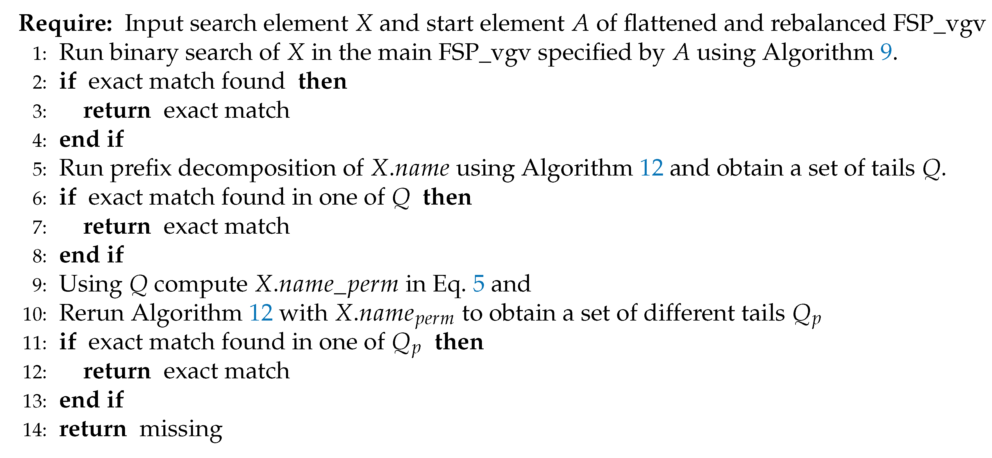
Figure 17.
Revised insert
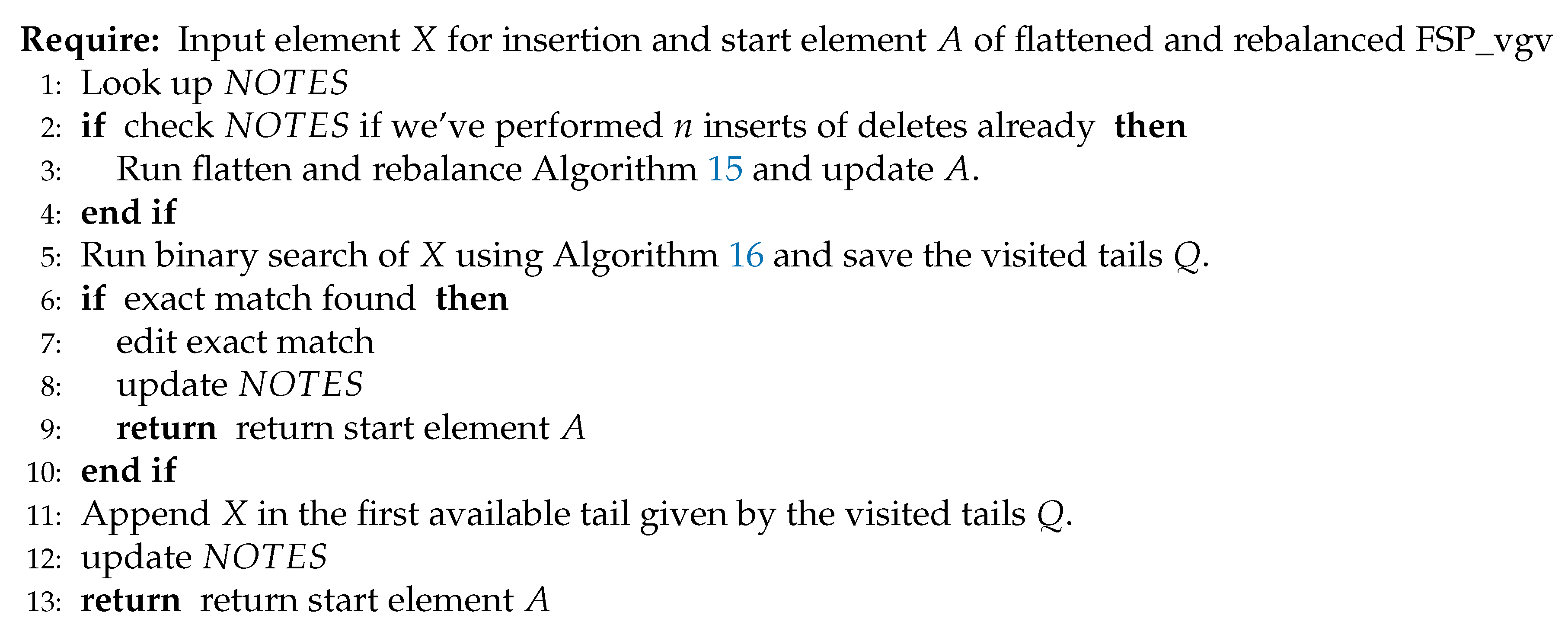
Figure 18.
Revised deletion
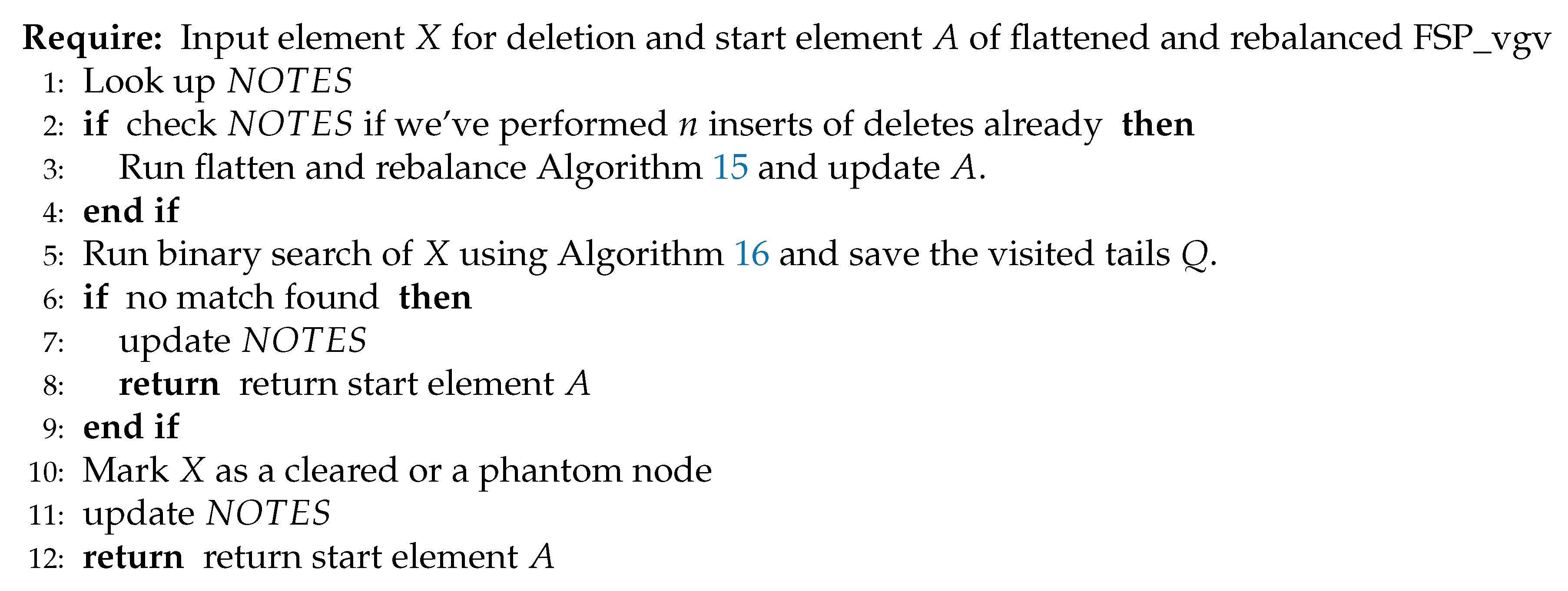
Figure 19.
Example of placing all variables in the same dynamic dictionary.
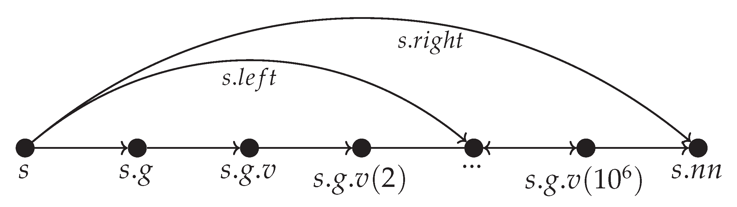
Figure 20.
Example of placing all variables in the same dynamic dictionary.
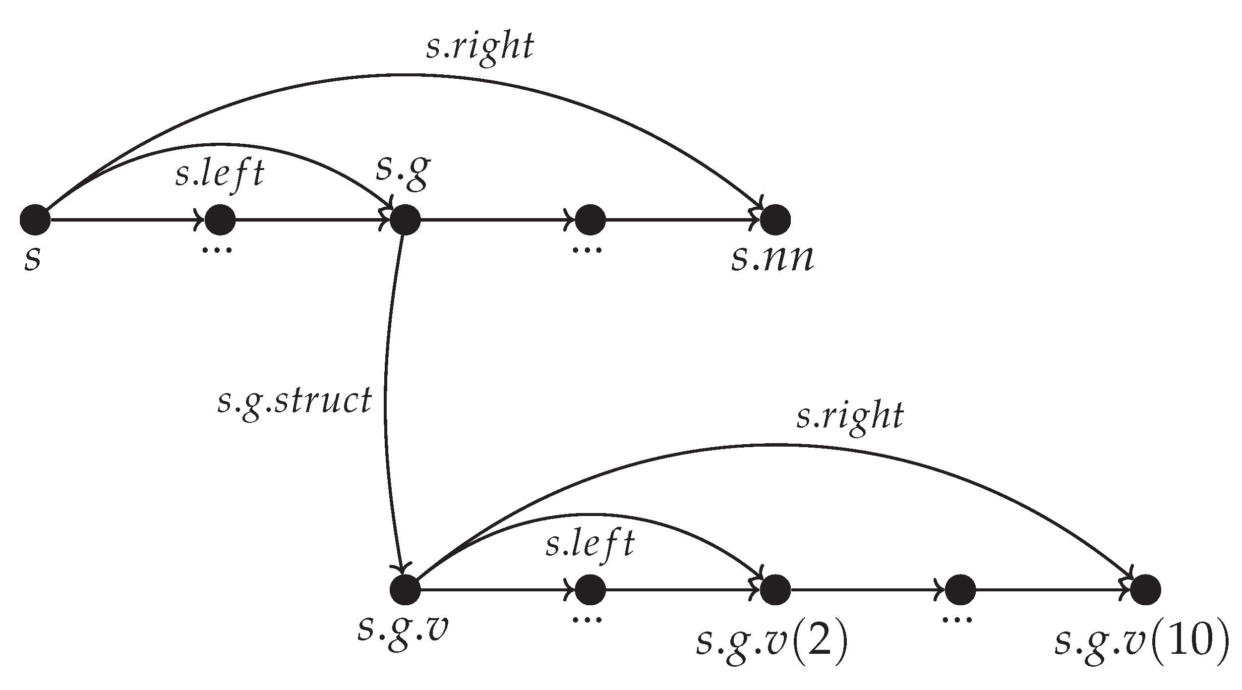
Figure 21.
Obseve that in this way we make use of the field without adding more fields to the class which improves memory management for large data sets.
Figure 21.
Obseve that in this way we make use of the field without adding more fields to the class which improves memory management for large data sets.
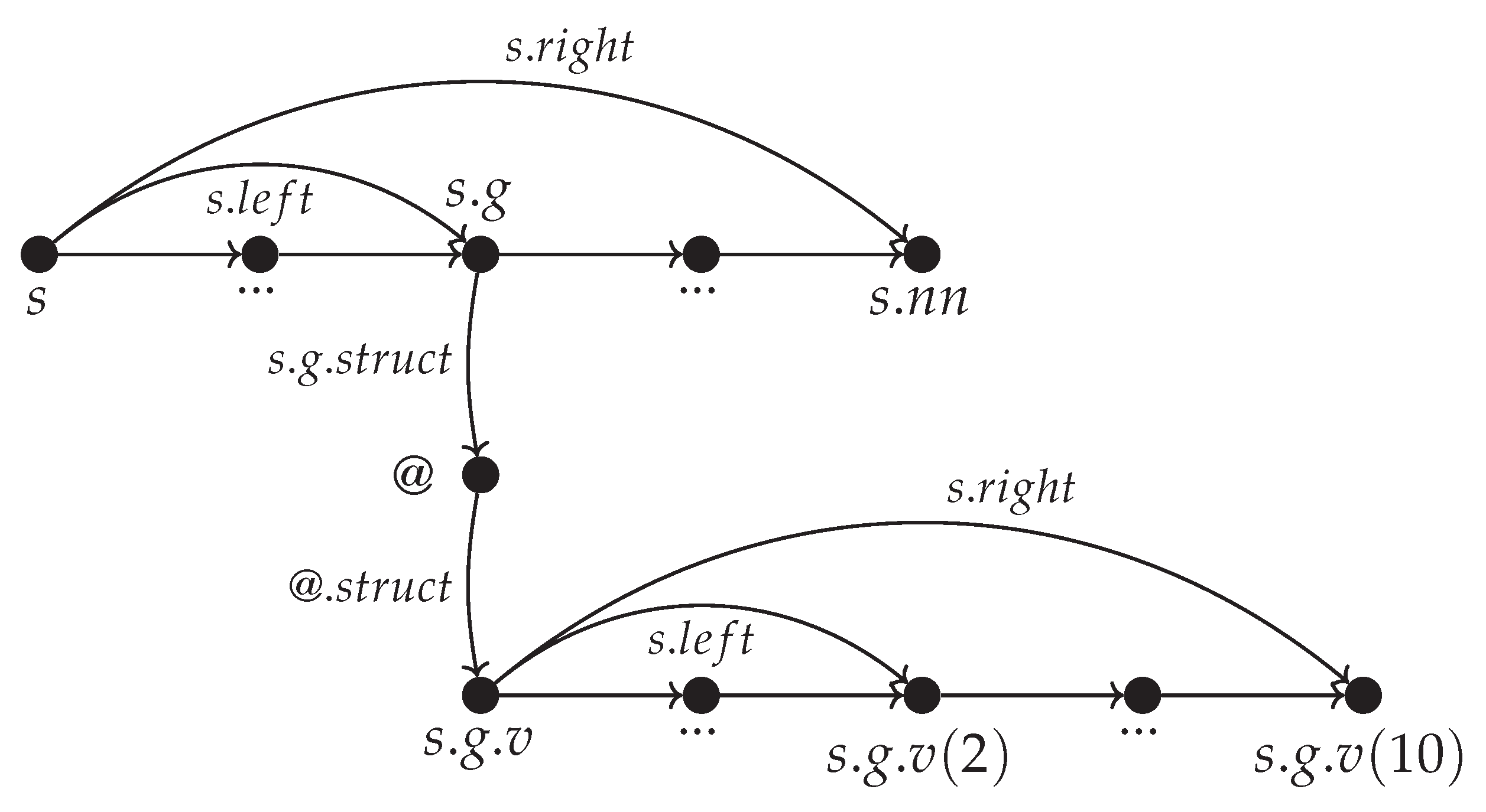
Figure 22.
Using a second FSP_vgv to enable time sensitive applications.
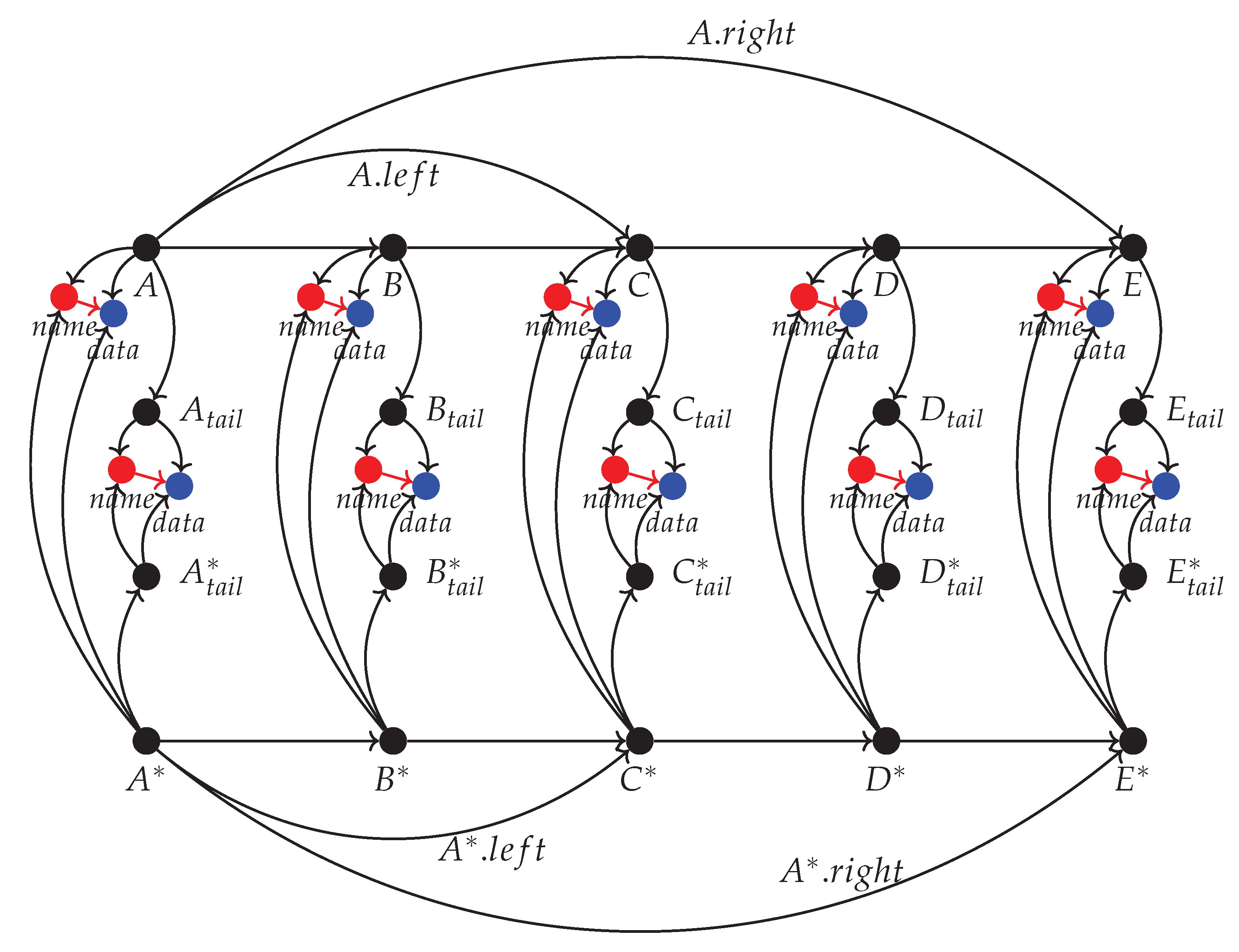
Figure 23.
First 200 versions.
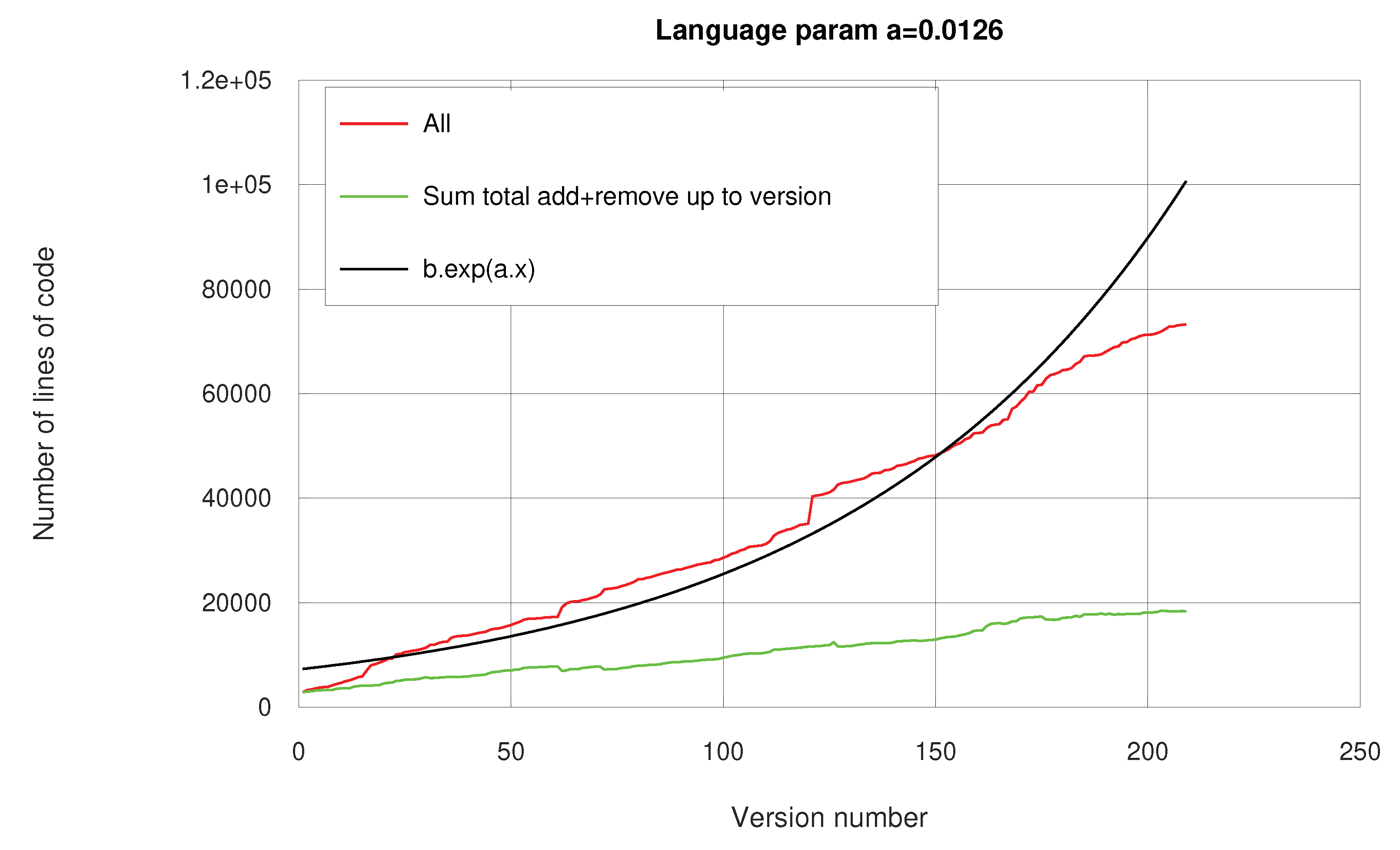
Figure 24.
Versions 200 till 600.
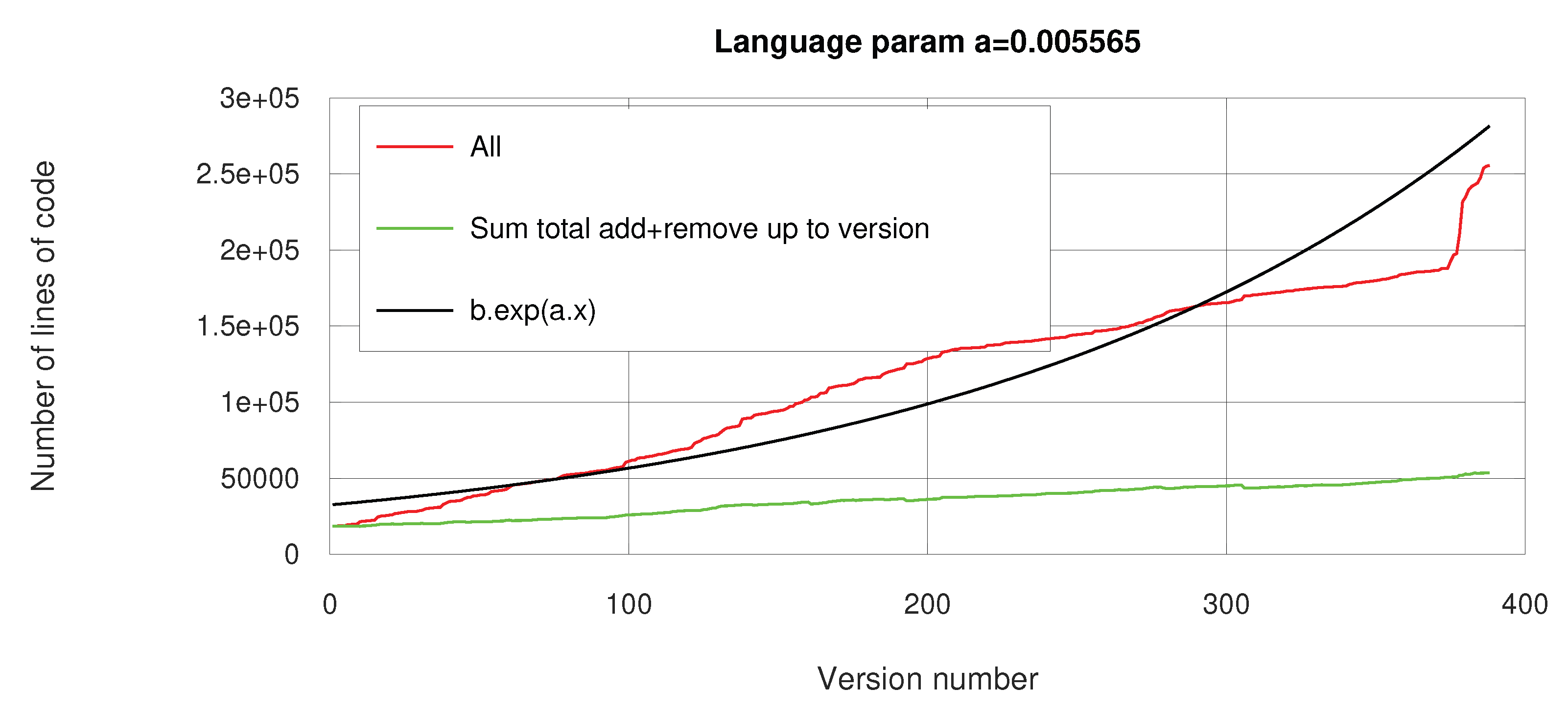

Table 1.
Prefix decomposition of n additional and unique elements
| Object | Permuted main prefix decomposition | |||||||
|---|---|---|---|---|---|---|---|---|
| Name | main prefix decomposition | permutation name | ||||||
| ... | ... | |||||||
| ... | ... | |||||||
| ... | ||||||||
| ... | ... | |||||||
| ... | ||||||||
| ... | ... | |||||||
| ... | ||||||||
| ... | ... | |||||||
Disclaimer/Publisher’s Note: The statements, opinions and data contained in all publications are solely those of the individual author(s) and contributor(s) and not of MDPI and/or the editor(s). MDPI and/or the editor(s) disclaim responsibility for any injury to people or property resulting from any ideas, methods, instructions or products referred to in the content. |
© 2026 by the authors. Licensee MDPI, Basel, Switzerland. This article is an open access article distributed under the terms and conditions of the Creative Commons Attribution (CC BY) license (http://creativecommons.org/licenses/by/4.0/).
Copyright: This open access article is published under a Creative Commons CC BY 4.0 license, which permit the free download, distribution, and reuse, provided that the author and preprint are cited in any reuse.


