
Submitted:
13 January 2026
Posted:
14 January 2026
You are already at the latest version
Abstract
As a core component of mechanical equipment, the operational status of bearings directly determines equipment safety, making early fault diagnosis critically important. However, bearing vibration signals are susceptible to substantial noise interference and exhibit both nonlinear and non-stationary characteristics, rendering traditional single-mode diagnostic methods ineffective at extracting fault features. Therefore, this paper proposes a three-channel multimodal fault diagnosis network (M-CNNBiAM) integrated with a convolutional autoencoder (CAE). Based on a convolutional neural network (CNN) architecture, this network employs CAE for signal denoising, utilizes continuous wavelet transform (CWT) to construct time-frequency features, and incorporates dual enhancement modules: convolutional attention (CBAM) and window attention (S-W-MSA).On one hand, it extracts complementary features from the raw vibration signal and the wavelet transform frequency domain signal, fusing them at the channel dimension. On the other hand, it embeds Shifted Window Attention (SW-MSA) and Window Self-Attention (W-MSA) between convolutional layers to capture global-local features. Combined with CBAM to enhance fault location attention, it mitigates the vanishing gradient problem through residual connections, enabling the extraction of frequency domain features. To address the characteristics of one-dimensional time-series signals, a bidirectional gated recurrent unit (BiGRU) is introduced to collaborate with CNN for extracting temporal features. Experiments demonstrate that on the West China University public dataset and self-test dataset, M-CNNBiAM achieves an average diagnostic accuracy of 95.84% under -10dB high-noise conditions, outperforming comparative methods and validating its superior performance in complex noise environments.
Keywords:
multimodal
; BiGRU
; CNN
; CBAM
; SW-MSA
; W-MSA
; CAE
1. Introduction
Bearings [1] are critical components in mechanical systems, including high-speed trains [2], aircraft [3], and CNC machine tools [4]. During operation, bearings frequently endure alternating loads and operate in complex environments, making them prone to failure. These failures often exhibit subtle early warning signs. Failure to detect them promptly may lead to equipment shutdown, structural damage, and, in severe cases, major safety incidents. Consequently, early fault detection is paramount. Conducting condition monitoring and intelligent diagnostics for rolling bearings has become a critical direction in ensuring stable equipment operation [5,6].
Traditional bearing fault diagnosis is based on an experience-driven method, which performs statistical calculations by analyzing the relationship between time and vibration quantities or by Fast Fourier Transformation (FFT) [7] into the frequency domain, and then completes the fault diagnosis by manual empirical judgement. These methods rely on manual experience and have insufficient ability to capture weak faults, and cannot cope with complex scenarios. Traditional fault-diagnosis methods no longer meet modern needs.
With the development of artificial intelligence, data-driven deep learning methods have become a research hotspot, and time-sequence and frequency-domain signal processing techniques are widely used [8]. These include CNN, BiGRU, Swin-transformer, CBAM, and Continuous Wavelet Transform (CWT). These methods are important in areas such as image recognition [9]. CNN [10] is a powerful network model well-suited for processing complex nonlinear signals and performs better on image data, thereby attracting significant attention in the field of fault diagnosis. Yin et al. proposed an improved Integrated Noise Reconstruction Empirical Modal Decomposition (IENEMD) combined with a parallel multiscale CNN fault diagnosis method for extracting fault features under noisy conditions [11]. Jang et al. proposed a CNN-based fault diagnosis method with high interpretability, converting the CNN output to a binary grey-scale image via singular value decomposition, and proposed an Average Score Drop (ASD) metric to quantify the interpretability of the analytical visualization method. The method can improve the interpretability of the CNN decision-making process while maintaining a high diagnostic accuracy [12]. BiGRU is a recurrent neural network with a gating mechanism, a variant of the Long Short-Term Memory Network (LSTM) that contains only reset and update gates, a design that is more lightweight while maintaining long-term memory capability [13]. Wang et al. proposed a GRU combined with a Residual Network (Res-Net) for fault diagnosis under time-varying operating conditions, achieving high fault diagnosis accuracy [14]. Jie Man et al. proposed a new form of axial temperature data organization, in which axial temperature measurement points are arranged as a graph according to specific positions. Then, using Graph Convolutional Networks (GCN) and the GRU model, it extracts features and predicts the axial temperature. Finally, the experimental results show that the prediction accuracy and tracking sensitivity are better than those of other state-of-the-art methods [15]. Swin-Transformer is a powerful tool proposed in recent years. It is improved based on Transformer by adopting the hierarchical structure of CNN and introducing SW-MSA and W-MSA, which breaks through the window limitation of Transformer and restricts the attentional mechanism to be computed only in the current window, which reduces the computation amount dramatically under the condition of guaranteeing that the model can obtain the global information [16]. An improved Transformer model was investigated by Lou et al. The model used a Swin-Transformer feature-extraction method by introducing new correction terms and constraints to reconstruct the loss function, thereby achieving more accurate uncertainty quantification in diagnostic prediction [17]. Zhou et al. proposed a novel multi-source information fusion network, the Feature Enhanced Variant Swin-Transformer (FEV-Swin), based on the Swin-Transformer framework, which incorporates a feature pyramid fusion module and a domain-adaptive module to achieve multi-source information fusion for fault diagnosis [18]. CBAM is a representative lightweight attention mechanism whose core architecture consists of a channel attention module and a spatial attention module connected in series. This dual-attention coordination mechanism guides the model to adaptively focus on critical feature regions related to bearing faults. By assigning higher weight coefficients to fault-sensitive information, it suppresses interference from irrelevant background noise and redundant features, thereby significantly enhancing the model's ability to detect subtle fault characteristics and improving the precision and effectiveness of feature extraction [19]. Qin et al. proposed a rolling bearing fault diagnosis method that integrates the CBAM attention mechanism with ResNet. By embedding the CBAM module into the residual block structure of ResNet, the attention mechanism enables adaptive focusing on critical fault features, effectively enhancing the model's feature extraction capability and fault identification specificity[20]. Xu et al. proposed a bearing-fault diagnosis method that integrates the CBAM attention mechanism with Inception Net. First, they decomposed the bearing vibration signal using Variational Modal Decomposition (VMD). Then, the processed signal was fed into a CBAM-enhanced Inception Net model, ultimately enabling effective bearing fault identification [21]. CWT is a classic time-frequency analysis method. Its core advantage lies in mapping one-dimensional time-domain signals into two-dimensional time-frequency matrices via convolution with adjustable-scale wavelet basis functions. This transform preserves the temporal dimension of the signal while precisely characterizing frequency distribution features at different time points. Consequently, it comprehensively captures the signal's joint time-frequency information, providing rich frequency-domain and time-correlation information to support subsequent fault-feature extraction [22]. Chen et al. designed a bearing fault diagnosis method integrating Resonant Sparse Signal Decomposition (RSSD) with Wavelet Transform (WT): First, RSSD decomposes the raw vibration signal, filtering out effective components containing fault information based on an energy criterion. Subsequently, WT reconstructs the filtered components, ultimately enabling deep extraction and diagnosis of bearing-fault features [23]. Cui et al. proposed a new method for shared frequency based on sparse analysis and wavelet transform theory. Fault diagnosis is achieved by assigning the shock signal frequency to multiple separation functions and finding shared frequency peaks in these separation functions to diagnose bearing faults [24].
Acquiring bearing vibration signals is prone to noise interference, and extracting fault features under strong noise conditions has gradually become a research hotspot. Wang et al. proposed a novel sparse representation (SR) model that employs generalized Gaussian distributions as basis functions. They designed the MoGG-SR algorithm based on expectation-maximization (EM) and alternating direction of multiplicity (ADMM), and experimental results showed that it outperforms several traditional denoising algorithms [25]. Li et al. employed an adaptive selection optimization method to optimize Feature Mode Decomposition (FMD) parameters, enabling the effective extraction of fault features in noisy environments [26]. Shen et al. designed a bearing fault diagnosis scheme for noisy conditions, integrating the Agile Grey Wolf Optimizer (AGWO), Particle Swarm Optimization (PSO), Variational Modal Decomposition (VMD), and the TEFCG-AlexNet convolutional neural network. The AGWO and PSO optimize the VMD decomposition parameters, and the resulting decomposed signals are then fed into the TEFCG-AlexNet for feature extraction and fault identification. Comparative validation against similar VMD-based algorithms demonstrates that the proposed method achieves optimal fault-diagnosis performance [27]. Zhao et al. proposed a Bidirectional Sparse Filtering (BiSF) method. The BiSF approach designed a novel bidirectional normalization strategy and incorporated a Squeeze-Enhance (SE) attention mechanism to adaptively weight input data and autonomously learn optimal weights. Experimental results demonstrate that, compared to traditional SF methods, the proposed BiSF method exhibits superior noise-suppression capabilities, effectively separating and eliminating noise components in vibration signals, thereby enhancing signal purity [28].
Although the aforementioned deep learning methods have demonstrated excellent performance in bearing fault diagnosis, significantly improving diagnostic efficiency and accuracy, they also exhibit certain limitations. For instance, CNNs suffer from local receptive fields, while K-SVD and Swin-Transformer algorithms consume substantial computational resources. Most denoising networks employ pre-processing denoising layers such as [25,26,27], signals must undergo pre-processing to reduce noise before undergoing image conversion or being converted into other data structures for input into neural networks for fault diagnosis. This approach is impractical for real-world deployment. The method proposed herein employs a neural network to simultaneously process both vibration signals and wavelet signals, facilitating the extraction of comprehensive fault information without requiring additional signal denoising, thereby enhancing practical deployability. First, the signal undergoes CWT to obtain its frequency-domain information, which is combined with the time-domain signal to construct a multimodal dataset. Frequency-domain features are extracted using a CNN incorporating SW-SAM and W-SAM, while time-domain features are extracted from the vibration signal using a CNN and BiGRU. Finally, the multimodal features are fused and fed into a classification layer for fault diagnosis. The main contributions of this paper are as follows:
- CNN Receptive Field Constraints: Incorporating SW-SAM and W-SAM into CNN layers restricts attention calculations within the current window while enabling cross-window connections to integrate global information.
- Feature Enhancement: Introducing CBAM after the window mechanism module forces the model to pay more attention to the fault site and enhances the model's ability to extract fault features.
- Multimodal fusion: fault features extracted from 2D frequency domain images and 1D time-series signals are fused to take full advantage of the complementary nature of these two types of data. The dual-channel data fusion enables the model to utilize time-frequency information simultaneously, thereby substantially improving fault classification accuracy.
- A CAE model was constructed to reduce noise signals. Experimental results demonstrated that in high-noise environments, CAE not only exhibits strong noise reduction capabilities but also achieves high efficiency.
2. Theoretical Foundations
This section details the principles of each component module within the proposed model and selects parameters for selected modules.
2.1. Convolutional Neural Network
Convolutional neural networks are deep feedforward neural networks that process data through local feature perception and hierarchical feature abstraction. They exhibit characteristics of regional connectivity, parameter sharing, and translation invariance. Local connectivity means hidden-layer neurons focus solely on specific local receptive fields; parameter sharing entails a single set of convolutional parameters shared throughout the entire feature extraction process; translation invariance ensures target features remain effectively recognizable even when their positions shift within the input. The unique structural design of CNNs significantly reduces the number of parameters through parameter sharing, effectively alleviating computational complexity during model training. The reduction in parameter redundancy inherently suppresses overfitting and enhances the model's generalization capability [29]. The basic components of a CNN include the input layer, convolutional layers, pooling layers, fully connected layers, and the output layer.
Convolution layers (also known as filters) serve as the core unit in the feature extraction stage of deep learning models. Essentially, they function as sliding feature-sensing windows that extract local key features from input data. By performing local connections and convolution operations between the convolution kernel and input data (such as images), convolution layers generate feature maps containing multidimensional feature information, laying the foundation for subsequent feature fusion and task decision-making. Figure 1 shows the structure of a CNN, and the convolutional operation can be expressed as follows:
where representing layer-level feature outputs. represents the i-th convolutional region of the l-1th layer feature map. and describe the parameters to be optimized during model training, including the weight and bias matrices for feature extraction. represents the activation function, which introduces nonlinearity to enhance the model's ability to fit complex features.
Pooling layers (also known as downsampling layers) are a critical component of feature processing in deep learning models. Their core function is to perform spatial dimension reduction on the high-dimensional feature maps output by convolutional layers. By employing dimension reduction strategies, they reduce the scale of feature data while effectively improving computational efficiency, reducing noise interference, and mitigating overfitting. Mainstream pooling operations include max pooling and average pooling: the former outputs the maximum value within a local sliding window, while the latter calculates the mean of all elements within the window. Both operations preserve and enhance key features, ultimately generating hierarchical features that represent the essential attributes of the data. The average pooling calculation formula is as follows:
(2)
represents the elements of the output feature map, denoting the average features of the window region; denotes the edge length of the pooling window, serving as a core adjustable parameter; m and n are indices; represents the original elements of the input feature map, constituting the processing targets of the pooling operation.
The maximum pooling calculation formula is as follows:
The fully connected layer (FC) achieves global feature fusion and deep mapping by combining extracted hierarchical feature vectors via a nonlinear function. After processing through the fully connected layer, feature information is transformed into a representation format tailored to the task requirements, with the final output produced by the output layer. The FC can be represented as:
Among them, b is the bias vector.
2.2. Gated Recurrent Unit (GRU)
The Gated Recurrent Unit (GRU) is a core variant of recurrent neural networks (RNNs), designed to address the gradient vanishing or exploding gradient issues that often arise when traditional RNNs process long sequence data. Compared to Long Short-Term Memory (LSTM) networks, GRUs employ a more streamlined gating structure, dynamically modeling temporal information solely through the update gate, reset gate, and current memory cell. Specifically, the update gate adapts the information transmission ratio, determining the proportion of new input information versus retained previous-step state in the current unit's state.
The reset gate controls the weight of the previous-step state, adjusting the influence of historical information on the current unit's state. The current memory cell generates new state candidate values based on the filtered historical data, as determined by the reset gate and the current input, ultimately completing the iterative update of temporal features. Figure 2 shows the gating mechanism, and the steps of the GRU gating principle are as follows [30]:
(1) Calculate the update gate represents the sigmoid function, with an output range of [0,1], used for gated "switch" control; and represent the parameter matrix, where corresponds to the weights of the input and corresponds to the weights of the hidden state; represents the bias vector, used for adjusting the offset in linear transformations.
(2) Calculate the reset gate(3) Calculate the candidate hiding statetanh represents the hyperbolic tangent activation function, with an output range of [−1,1], used for feature mapping of candidate states;⊙denotes element-wise multiplication, enabling per-element weight adjustment. represents the newly generated candidate state value based on the current input and resets historical information.
(4) Update the hidden status represents the integration of historical information and the current candidate state, outputting the temporal feature representation for the current time step.
2.3. Swin-Transformer Block
The core innovation of Swin-Transformer lies in introducing a sliding window attention mechanism. This breaks away from the Transformer's limitation of calculating attention only within the current window, enabling cross-window connections. This significantly enhances the model's ability to learn global semantic relationships while balancing the locality of feature extraction with global contextual dependencies. The sliding window attention mechanism first divides the input feature map into non-overlapping local windows. Within each window, W-MSA captures local features, while window shifting enables information exchange between adjacent windows to establish global dependencies, effectively reducing the computational complexity of traditional Transformers. As the fundamental building block of the model, the Swin Block comprises W-MSA, SW-MSA, and a Multi-Layer Perceptron (MLP). Figure 3 shows the Block layer structure. Block computation can be represented as [31]:
Where represent the S(W)-MSA output features and MLP output features of the -th Block, respectively.
The structure of the Multi-Head Self-Attention mechanism (MHSA) in Swin-Transformer is shown in Figure 4, and the computation can be expressed as:
Where and represent the query matrix, key matrix, and value matrix, respectively.
2.4. Convolutional Block Attention Module (CBAM)
CBAM [32] is a simple, lightweight attention mechanism that is often combined with convolutional networks or visual Transformers to enhance feature representation. At its core, CBAM achieves precise focusing and adaptive refinement of key features by serially coordinating channel and spatial attention, addressing both "which features are important" and "where features are important." This effectively enhances the model's ability to perceive global semantic information and local detail features jointly. Figure 5 shows the CBAM structure.
(1) Channel Attention Branch: Primarily addresses the question of "which features are more critical," focusing on feature selection at the channel dimension. This branch first performs global average pooling and global max pooling on the input feature map, comprehensively capturing channel-wise feature distribution information through dual pooling. Subsequently, the pooled results are fed into an MLP to learn dependencies among channels, ultimately producing a channel-weight map. This highlights the feature contributions of key semantic channels while suppressing redundant channel information. Figure 6 shows the channel attention module. The channel attention mechanism can be expressed as:
represents the attention weight for each channel; denotes the input feature map; is the Sigmoid function, mapping the MLP output to weight values; represent average pooling and max pooling, capturing global average information and salient feature information across channels, respectively; denotes the enhanced channel feature map, preserving key channel information while suppressing redundant channel interference; indicates element-wise multiplication.
(2) Spatial Attention Branch: Focusing on the question of "where features are more critical," this branch takes the feature map output from the channel attention as input and performs average pooling and max pooling operations along the channel dimension. By learning spatial positional dependencies through convolutional layers, it generates a two-dimensional spatial attention map that guides the model to focus on the target's key regions precisely. Figure 7 shows the spatial attention module. The spatial attention module is represented as:
2.5. Wavelet Transform
CWT [33] calculates the similarity between the original signal and wavelet basis functions at different scales and time-domain positions by adjusting the scale factor and shift amount, thereby constructing a two-dimensional time-frequency feature matrix. The core advantage of this transform lies in overcoming the technical limitations of the Fourier Transform (FT) — FT can only capture the global frequency-domain distribution of a signal and cannot reflect the temporal evolution characteristics of frequency components, resulting in the loss of critical local temporal information. In contrast, CWT achieves a joint representation of the signal's local temporal features and frequency-domain distribution patterns through the synergistic interaction of scale factors and translation amounts, enabling adaptive analysis of non-stationary signals. The principal steps of the wavelet transform are as follows:
- (1) Wavelet basis function construction
- (2) Calculate the wavelet coefficients
- (3) Construction of time-frequency images
The wavelet coefficients calculated are arranged into a two-dimensional matrix according to scale factors and translation factors to construct the time-frequency image.
Figure 8.
Wavelet Time-Frequency Images for Bearing Fault Diagnosis.
2.6. Autoencoder
AE compresses input signals through an encoder to map them into a low-dimensional space. The decoder reconstructs the signals from this low-dimensional space back to their original dimensions, striving to maintain maximum consistency between the reconstructed signals and the original signals [34]. Since noise exhibits random distribution across all frequencies, while fault signals typically follow periodic impact patterns, AE is particularly well-suited for bearing vibration signal denoising tasks. The AE structure is shown in Figure 9, and signal decoding and encoding can be expressed by the following equations.
Encoding Operations:
Decoding operation:
Among these, represents the feature map of layer l; denotes the activation function; denote the input signal and output signal, respectively; and denote the stride, padding, and bias, respectively.
3. M-CNNBiAM Model
This section provides an introduction to M-CNNBiAM and gives model-specific parameters, structural diagrams, data dimension change tables, and model diagnostic procedures.
The M-CNNBiAM architecture is shown in Figure 9, with the process divided into four steps: 1. Noise addition, 2. Construction of time-frequency data 3. Feature extraction 4. Fault classification Table 1 and Table 2: Module parameter tables; Table 3: Image feature extraction; Table 4: Vibration signal feature extraction.
- (1) Noise addition
This paper added Gaussian noise with SNR values of [-10, -8, -6, -4, -2, 0, 2, None] dB to the original vibration signal and verified the accuracy of the noise addition.
- (2) Constructing time-frequency data
The noise signal first enters the CAE for denoising, with the specific structure of the designed CAE shown in Figure 11. The denoised signal is converted into a frequency domain image via CWT, using the complex Morlet wavelet with a bandwidth parameter of 100 and a center frequency parameter of 1. The CWT signal and vibration signal together form a multimodal dataset.
- (3) Feature extraction
The image data first undergoes channel expansion via a convolutional kernel of sizewith stride 2, followed by image size reduction to decrease computational complexity. The preprocessed signal enters a dual-parallel image branch. Data entering Image Branch 1 sequentially passes through three layers of a convolutional neural network (ResNetBlock) with kernel size and stride 1. This is followed by a window attention module and CBAM, with the output features re-entering ResNetBlock to generate final features. Branch 2 shares the same architecture as Branch 1, except its first three CNN layers use a kernel size of , while all other parameters remain identical. Finally, features are concatenated to produce frequency-domain modal features. Vibration signals first undergo dimension reduction and channel expansion via a convolutional layer with kernel size and stride 2. It then sequentially passes through a convolutional layer with kernel size , a ResNetBlock, and the output features enter a BiGRU with [32,64] neurons to generate time-domain modal features. All CNN layers are followed by batch normalization (BN), a ReLU activation function, and a dropout layer. Finally, the time-domain feature (F3) and frequency-domain features (F1, F2) are concatenated along the channel dimension to obtain multimodal features.
- (4) Fault Classification
Multimodal features are concatenated along the channel dimension before entering the classification layer for classification, enabling fault diagnosis.
In Figure 11, the noisy signal first enters a three-layer convolutional layer with kernel sizes [7,5,3]. It then undergoes deconvolution to complete the encoder output. Subsequently, the signal undergoes deconvolution to enter the decoder. The decoder performs three layers of transposed convolutions with kernel sizes [3,5,7], followed by deconvolution to output the denoised signal. The main hyperparameter settings for CAE are as follows: Iteration count: 320 Loss function: MSE loss Learning rate: 0.0001.
Figure 10 shows that the wavelet signals enter the preprocessing CNN in parallel to adjust the input dimensions for the subsequent CNN. They then pass through three ResNetBlocks. The first branch employs large kernels with a larger receptive field, enabling coverage of broader image regions. This configuration is suitable for capturing global structural features while offering stronger suppression of large-scale noise. Residual connections are employed to prevent gradient vanishing. Features then enter the Swin-Transformer Block. W-MAS restricts computations to the current window, reducing computational load, while SW-MAS permits cross-window connections to capture global information. Features subsequently undergo CBAM to further focus on fault locations before entering the final ResNetBlock for dimension adjustment and feature output. The small kernel branch features a narrower receptive field, excelling at capturing local detail features while preserving finer information. Its heightened sensitivity to small-scale noise facilitates precise filtering. This dual approach covers multi-scale features from local to global, avoiding the one-dimensional feature capture inherent in single-scale convolutional kernels. The temporal domain employs five ResNetBlocKs with stride control. The first three layers suppress noise while capturing long-term dependencies, while the latter two extract global features, covering the full spectrum from macro trends to micro-transients. Each convolutional layer utilizes residual connections. The temporal features finally enter a BiGRU to prevent long-term sequence forgetting. The gating design of BiGRU inherently possesses noise resistance, further mitigating residual noise effects. The three-channel features are concatenated along the channel dimension before entering the classification layer. To mitigate overfitting in complex models, Dropout2d=0.1 is applied after each convolutional layer in the image branch. Dropout1d=0.1 follows the five convolutional layers in the time-domain branch, with Dropout1d=0.2 after the BiGRU. The final fusion layer employs Dropout1d=0.5, effectively preventing overfitting.
4. Experiments and Results
This section validates the proposed model's generalization capability and diagnostic accuracy through two sets of comparative experiments. Testing was conducted using both the Case Western Reserve University (CWRU) standard bearing-fault dataset and a simulated operating-condition dataset, ensuring coverage of both real-world and controlled simulated fault scenarios to enhance the reliability of the conclusions. To comprehensively evaluate model performance across multiple dimensions while quantifying the impact of hyperparameters on diagnostic effectiveness, the following core evaluation metrics were selected:
First, accuracy, precision, recall, and F1-score are employed. Accuracy reflects the model's overall classification correctness; precision measures the reliability of predictions; recall indicates the ability to identify target faults and reduce missed diagnoses; and the F1-score, as the harmonic mean of the two, balances comprehensive classification performance in imbalanced sample scenarios. Additionally, runtime and parameter count are included. Runtime is the total time for one training cycle and reflects training efficiency. Parameter count represents the total number of learnable parameters in the model, measuring model complexity and storage overhead. Finally, a confusion matrix visually presents the classification results. Rows correspond to the actual fault categories of samples, columns represent the model's predicted categories, and element values indicate the number of classifications for each category. This clearly identifies the correct classification status and misclassification types for various faults, providing a clear direction for model optimization. The hyperparameters of this model are set as follows: the learning rate is 0.0005; the optimizer is AdamW; Weight decay is 1e-4, and the number of training rounds is 50.
The experimental platform is configured with an Intel Core i5-13450HX CPU, 16 GB of RAM, an RTX 4060 graphics card, and the PyTorch (V3.11.7) deep learning framework for model training and experimental validation.
4.1. Noise Addition and Noise Reduction Effect Verification
To better simulate the high noise levels present in real-world working environments, Gaussian noise is added to the original signal. The signal-to-noise ratio (SNR) can be expressed as:
(15)
Among these, represents the original signal; represents the added noise power.
The noise added in the experiment is Gaussian noise. To verify the effectiveness of noise addition, the spectrum diagram, time-domain vibration diagram, and continuous wavelet transform diagram are provided. Taking a Gaussian noise signal with SNR = -6 dB as an example.
Figure 11 shows a frequency domain comparison of the signals. The frequency domain provides a more intuitive view: the original signal exhibits distinct peaks. In contrast, the signal with added mixed noise exhibits an irregular spectrum spanning the entire frequency band. The noise completely obscures the fault information, rendering the signal complex.
Figure 12.
Signal Frequency Domain Comparison Diagram.
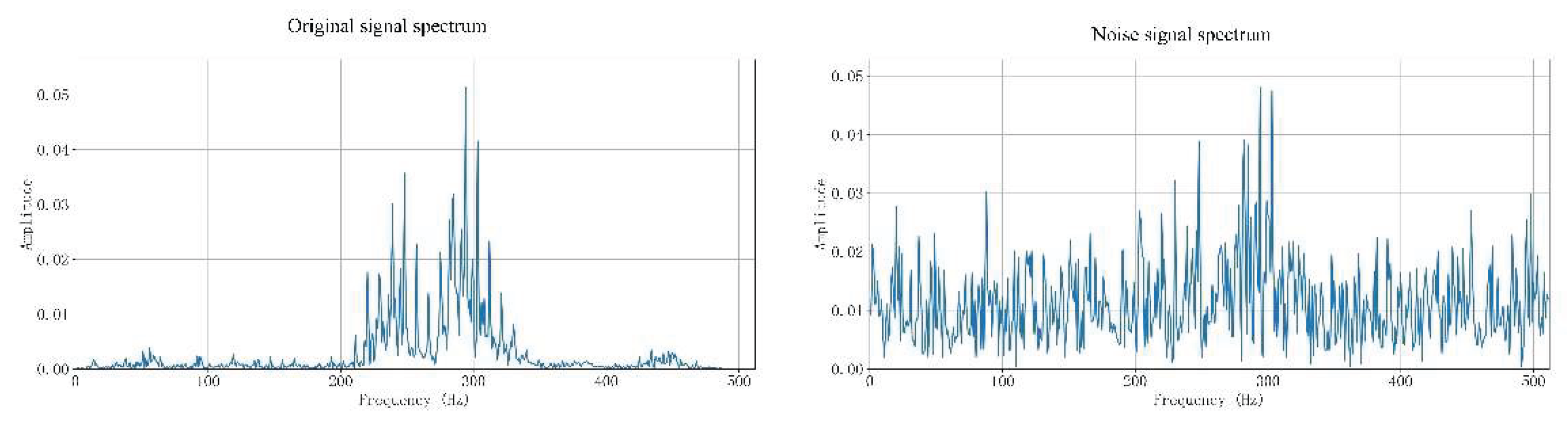
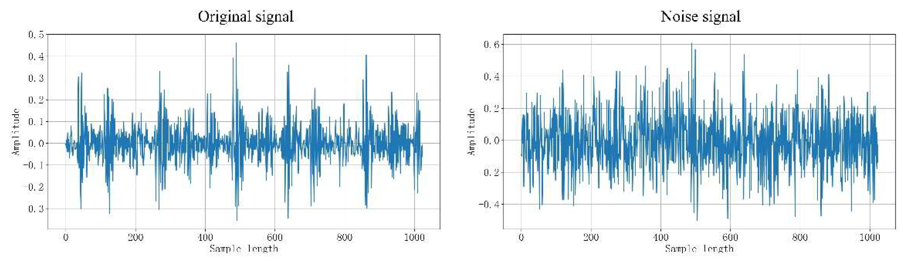
Figure 13.
Vibration Signal Comparison Chart.
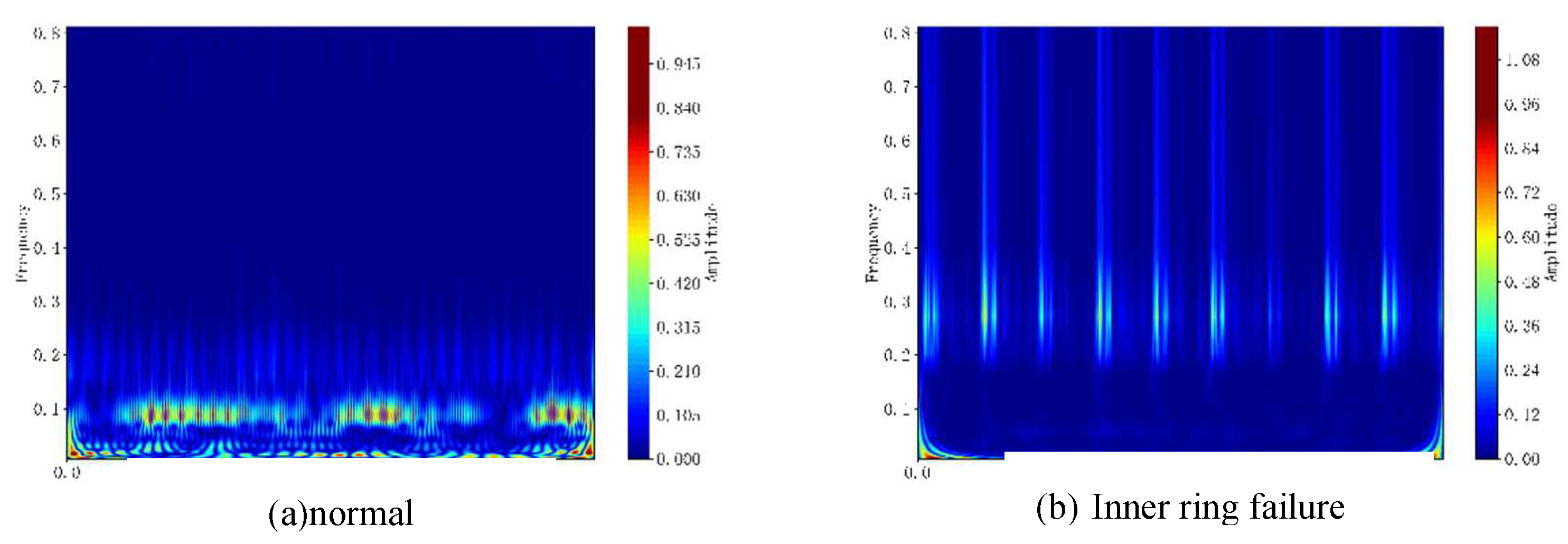
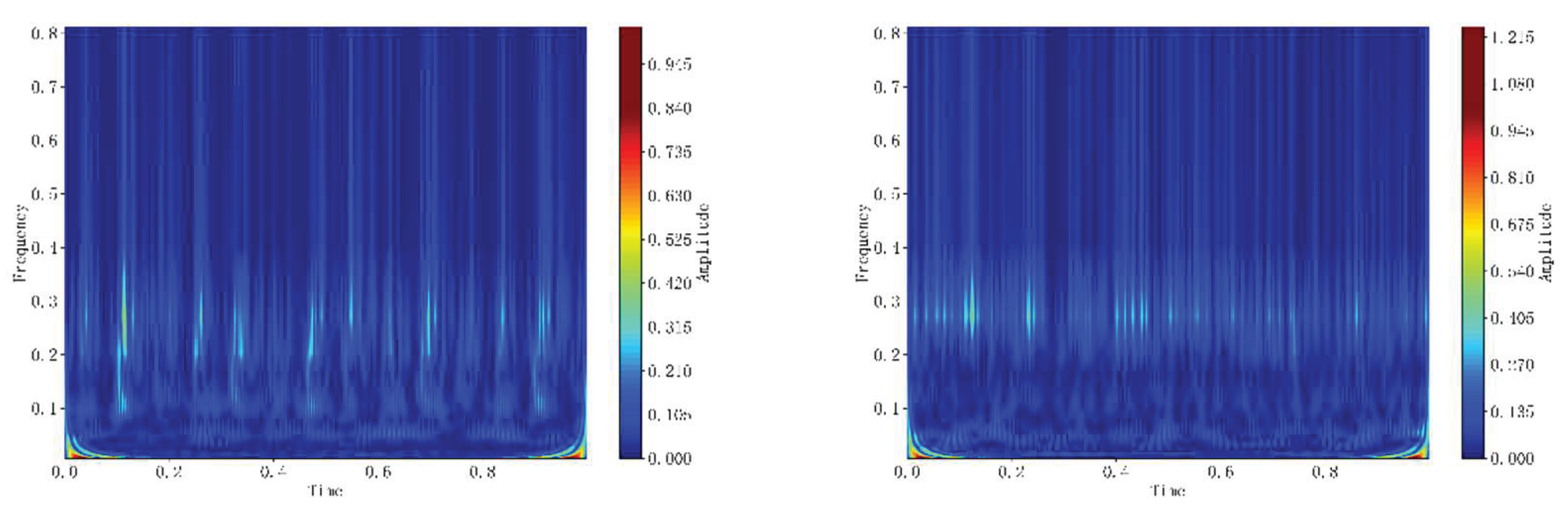
As shown in Figure 14, the periodic pattern of the original vibration signal in the time domain is preserved after CWT transformation, appearing as banded stripes. Peak values in the frequency domain manifest as red dots at specific locations, indicating where larger wavelet coefficients were assigned by the CWT. Through time-frequency complementarity, this approach enables the model to capture comprehensive fault characteristics, enhancing its generalization capability and diagnostic effectiveness.
To validate the noise reduction effectiveness of the autoencoder, we visualized the signal's envelope spectrum. As shown in Figure 15, the red-boxed section represents noise, which has completely obscured the signal's fault frequency. After noise reduction using the autoencoder designed in this paper, we observe that the fault features are perfectly restored. Compared to the envelope spectrum of the original signal, only very faint noise remains. To verify the gap between the denoised signal and the original signal, we use the MSE metric as shown in Figure 16. The MSE of the original signal is 0.08, while the MSE of the denoised signal is 0.11, fully validating the noise reduction capability of the proposed AE.
4.2. Case Western Reserve University Experimental Data
The CWRU dataset includes inner-race, outer-race, and rolling-element faults. Each fault type comprises three fault sizes (7, 14, and 21) plus a normal state, collectively forming ten distinct files. Bearing vibration signals were collected at 12 kHz. For the experimental samples, the single-sample length was set to 1024, with a data overlap rate of 0.5 to utilize the data and avoid feature redundancy fully. The dataset was randomly partitioned into training, validation, and test sets at a ratio of 7:3:1. The training set was used for model parameter learning, the validation set for hyperparameter tuning and overfitting monitoring, and the test set for evaluating model generalization performance. Detailed information regarding the experimental data is presented in Table 5.
To validate the fault diagnosis performance of the proposed model, experiments were conducted using the CWRU bearing dataset. Table 6 lists the core evaluation metrics of the model. As shown in Table 6, even under extremely high noise levels of -10dB, the model maintains an accuracy rate of 98.57%. We visualized the confusion matrix to better analyze the model's classification capability for fault categories. As shown in Figure 17, the misclassified data points in the confusion matrix are broadly dispersed rather than clustered within specific categories. This indicates the model possesses strong diagnostic capability and demonstrates reasonable robustness, exhibiting low sensitivity to specific fault types. Figure 18 shows the T-SNE visualization for reference. To further examine the model's decision-making process during training, we visualized the training curve in Figure 19. The model's training exhibited minimal fluctuation overall, achieving high accuracy by the 10th iteration. By the 20th iteration, the training and validation curves converged, indicating optimal diagnostic performance. The subsequent 30 iterations proceeded smoothly without overfitting. This performance stems from residual connections ensuring stable gradient propagation, coupled with a cosine annealing strategy for learning rate scheduling. This approach guarantees more stable and rapid optimization toward the optimal parameter combination.
4.2.1. Comparative Experiment
To validate the superiority and stability of the proposed model, it will be compared with other advanced models. Table 7 presents the evaluation metrics for the comparison models. Qiao et al. proposed a dual-input neural network model combining CNN and LSTM. This model incorporates time-frequency signals as input using mini-batch and batch normalization techniques. On the Case Western Reserve University Experimental Data dataset, it achieved high fault recognition rates under noisy conditions while demonstrating robust noise immunity and load adaptability [35]. Zhang et al. proposed a fault diagnosis model integrating wavelet denoising with the KANTransformer. The front-end employs a wavelet denoising module to filter redundant noise from the raw signal, providing a high-quality data foundation for feature extraction. The core innovation lies in the KANTransformer's introduction of learnable activation functions within its linear layer, overcoming the expressive limitations of traditional fixed activation functions and significantly enhancing the model's ability to capture nonlinear and non-stationary characteristics of fault signals. Experimental validation demonstrates the model's outstanding resistance to interference under complex noise conditions, enabling effective differentiation between noise and fault features while achieving excellent fault diagnosis accuracy and robustness [36]. Shi et al. proposed an EWSNet network algorithm that introduces a wavelet-weight initialization method and a balanced dynamic adaptive thresholding algorithm, demonstrating the network's effectiveness and reliability across four datasets [37]. Zhang et al. proposed a small-sample fault diagnosis method combining dual-path convolution with attention (DCA) and bidirectional gated recurrent units (BiGRU) for noisy conditions and variable operating scenarios. This model achieves fault diagnosis by integrating spatio-temporal features using a regularization-based training strategy coupled with BiGRU. Results demonstrate that the model exhibits strong generalization capabilities and robustness[38]. All models were compared under a -4 dB noise condition. Figure 20 shows the bar chart of accuracy rates for the comparative experiments.
Figure 20 demonstrates that models (a) and (b) exhibit high diagnostic accuracy under strong noise conditions (SNR = -4 dB), both achieving over 99%. This is attributed to the inclusion of pre-denoising modules in both models, which process signals before network input and complete denoising—such as the wavelet denoising employed in method (b)—thereby maintaining high diagnostic precision. Although models (c) and (d) exhibit slightly lower accuracy under noisy conditions, they were tested on small sample sizes. The results presented in the paper were obtained using 150 samples, which represents the maximum sample size in the study. Generally, accuracy improves to some extent as the sample size increases. Therefore, under the same sample size conditions, the models (c) and (d) may demonstrate superior diagnostic performance.
The aforementioned models each possess distinct advantages; however, most denoising network models rely excessively on data preprocessing while neglecting the inherent denoising capabilities of the model itself. Furthermore, when relying on neural network models for denoising under extremely high noise conditions, training becomes unstable and requires significantly longer training times. Therefore, if the model itself can exhibit a certain degree of noise resistance under low-noise conditions, it would be more advantageous for practical deployment. Consequently, this paper tested the model solely through its core architecture under noise conditions of [[-4, -2, 0, 2], with results shown in Table 8. The model achieved 94.42% accuracy even at -4dB, which is acceptable for engineering applications, while exhibiting relatively stable training fluctuations overall. Thus, the proposed model demonstrates significant advantages. Figure 21 displays the training curve at -4dB,Figure 22 shows the confusion matrix.
4.2.2. Melting Experiment
To more clearly demonstrate the contribution of each model module, ablation experiments were conducted on the Xicheng University dataset at SNR=-4dB. The specific ablation models are detailed in Table 9. Model-1 includes only the first image branch, Model-2 includes only the second image branch, Model-3 includes only the time-domain branch, and Model-4 incorporates the entire image branch. Compared to Model-5, Model-4 lacks the Windows-Attention module, while Model-6 omits the CBAM module relative to Model-2. Table 10 lists the evaluation metrics, and Figure 23 displays the confusion matrix.
4.3. Simulated Bearing Data
The acquisition parameters and operating conditions for the simulated dataset used in this section are as follows: The sampling frequency of the dataset is set to 20 kHz to ensure accurate capture of high-frequency fault feature signals during bearing operation. The 6007 deep groove ball bearing was selected as the research subject, with its rotational speed stably maintained at 1500 rpm to simulate typical medium-to-low speed operating conditions in industrial scenarios. The dataset encompasses four critical bearing operating states: normal operation, inner ring failure, outer ring failure, and rolling element failure, constituting a four-class fault diagnosis task. Detailed information on the simulated dataset is presented in Table 11, while Figure 24 shows the physical layout of the simulation test bench used for data acquisition.
4.4. Number of Parameters and Timeliness of the Model
In industrial deployment scenarios, the parameter efficiency and real-time response capability of fault diagnosis models are core indicators determining their engineering applicability, directly impacting the timeliness of fault diagnosis and the feasibility of hardware deployment. To validate the engineering potential of the proposed model, the West China University Bearing Dataset was employed as the test subject. Each vibration signal in this dataset spans 1024 points, comprising 2330 valid samples. The model's timeliness was assessed by measuring its single-run processing time. The statistical results of the model's parameter count are shown in Table 13 and Table 14. It can be seen that the overall parameter count of the proposed model is at an intermediate level within the industry, without excessive redundancy, providing the fundamental conditions for lightweight deployment. However, as shown in Table 15, the average single-round runtime of the model is 6.8 seconds. This is due to the high computational complexity of the Block's window attention mechanism. Nevertheless, the 6.8-second runtime offers significant advantages in practical applications. On one hand, the fault evolution process of rolling bearings typically involves specific time scales, and a 6.8-second diagnostic delay enables rapid response to fault warnings, facilitating subsequent maintenance decisions. On the other hand, in industrial settings, runtime can be further reduced through hardware computing power upgrades or algorithm optimization. Therefore, this model retains high application value for practical industrial deployment.
4.5. Interpretability of the Model
Model interpretability is crucial as it helps us understand how models make decisions, enhances their credibility, and facilitates targeted improvements. To explain how CNNs extract fault features, we visualized the weight maps of the five convolutional layers in the vibration signal feature extraction pipeline. These five layers comprise the preprocessing convolutional layer and the final convolutional layers within the four residual blocks. As shown in Figure 26, darker colors indicate larger weights. The figure reveals that the first three convolutional layers assign greater weights to the fault location, demonstrating that the model has learned fault patterns and effectively identifies fault features. The subsequent two convolutional layers incorporate global features, fully validating the model's feature extraction capabilities and global temporal modeling abilities.
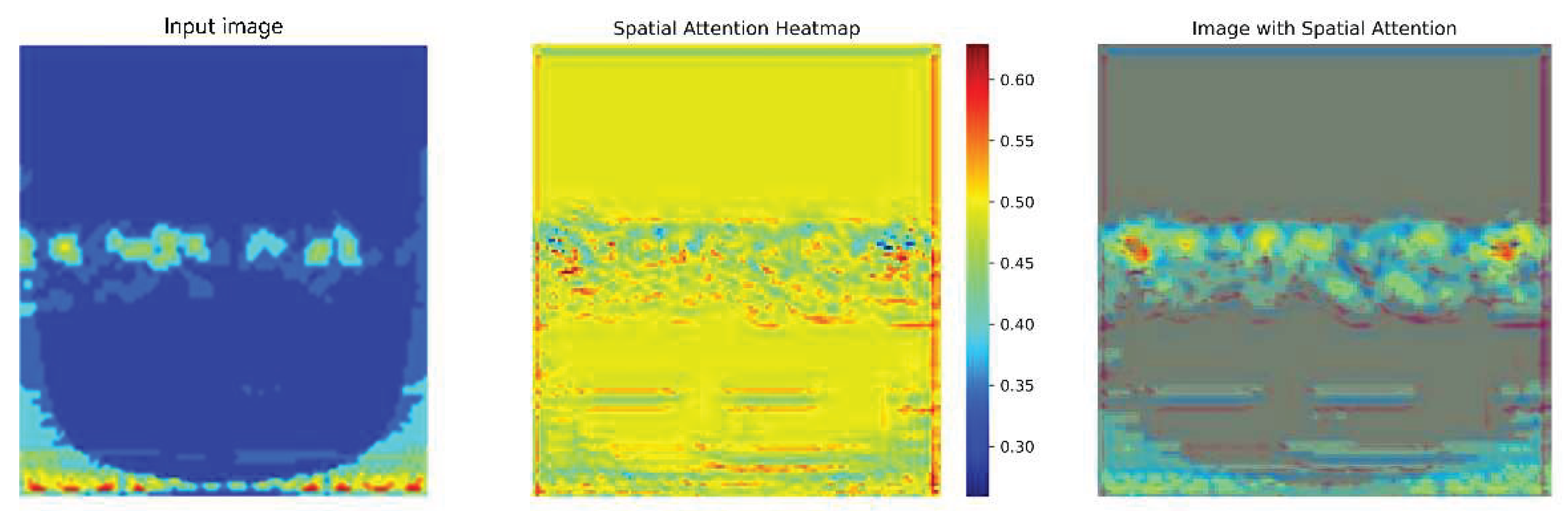
Understanding how attention mechanisms enable models to capture fault features accurately is a core issue in bearing fault diagnosis. To visually validate the operational principles and model interpretability of both channel and spatial attention mechanisms, this paper employs heatmaps visualizing feature responses. These heatmaps demonstrate that brightness (color intensity) positively correlates with attention weights—i.e., higher brightness indicates a greater contribution to fault diagnosis. The bar chart in Figure 21 reveals significant variations in attention weights across feature channels. The differing importance distributions of channels across model module positions demonstrate that the model dynamically adjusts its focus on channels in response to task requirements during feature processing. This confirms the core capability of channel attention: the model automatically learns and highlights channels more useful for the task. This mechanism enhances fault-feature extraction accuracy and diagnostic reliability by adaptive feature-channel filtering. The spatial attention heatmap in Figure 22 indicates that the model automatically assigns high weights to regions in the wavelet transform (CWT) feature map directly related to faults. This demonstrates that spatial attention precisely localizes and amplifies fault-specific features in the spatial domain, thereby improving the distinguishability between fault and non-fault features, highlighting its value within the model.
Figure 27.
Channel attention weights.
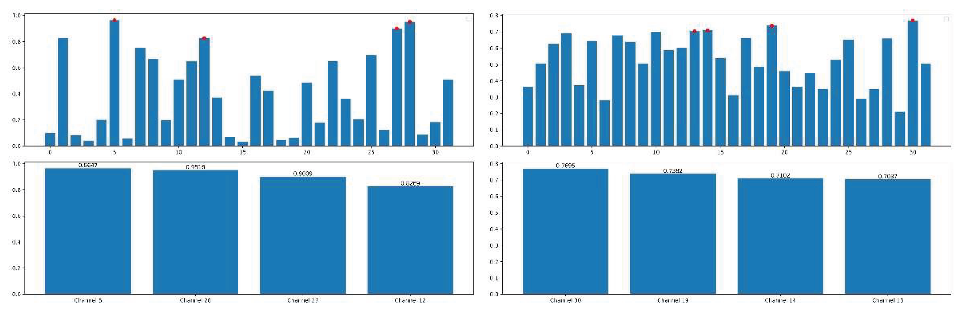
Figure 28.
Spatial attention weights.
5. Conclusions
This paper proposes a three-channel M-CNNBiAM multimodal hybrid model integrating image and vibration signals to achieve multimodal feature fusion for bearing fault diagnosis in complex scenarios. To address the challenge of extracting fault features from strong noise, an autoencoder is designed for signal denoising, maximizing the restoration of fault signals. The model combines CNN with window attention mechanisms to overcome the limitations of deep CNNs in handling restricted receptive fields and global information association. It further incorporates CBAM attention to effectively capture spatial features in image data. A 1D CNN and bidirectional GRU network are employed to specifically extract long-term dynamic features from vibration signals. Finally, multimodal feature fusion leverages complementary information from images and vibration signals to achieve fault diagnosis. Experimental results demonstrate the proposed model's outstanding classification performance on both the Xicheng University dataset and simulated experimental datasets. It effectively extracts fault features even under high-noise conditions, outperforming both single-modal models and traditional fusion methods. Visual analysis of channel attention weights and spatial attention weights verifies the model's adaptive focus on critical features, demonstrating the effectiveness of the attention mechanism. Visualization of convolutional layer weights enhances the model's interpretability. Future work may further optimize the cross-modal attention mechanism design, explore more powerful feature interaction methods, and extend the model's application to more practical scenarios such as industrial monitoring and fault diagnosis.
Author Contributions
Conceptualization, YY.Z. and CF.L.; methodology, YY.Z., CF.L. and Y.Z.; software, CF.L.; validation, CF.L., Y.Z and ZQ.S.; formal analysis, CF.L.; investigation, CF.L. ;resources, CF.L.; data curation, L.L. and ZQ.S.; writing—original draft preparation, CF.L.; writing—review and editing, CF.L.,ZQ.S.,Y.Z. and L.L.; visualization, ZQ.S. ; supervision ,YY.Z.; project administration, YY.Z.; funding acquisition, YY.Z. All authors have read and agreed to the published version of the manuscript. Conceptualization, YY.Z. and CF.L.; methodology, YY.Z., CF.L. and Y.Z.; software, CF.L.; validation, CF.L., Y.Z and ZQ.S.; formal analysis, CF.L.; investigation, CF.L. ;resources, CF.L.; data curation, L.L. and ZQ.S.; writing—original draft preparation, CF.L.; writing—review and editing, CF.L.,ZQ.S.,Y.Z. and L.L.; visualization, ZQ.S. ; supervision ,YY.Z.; project administration, YY.Z.; funding acquisition, YY.Z. All authors have read and agreed to the published version of the manuscript.
Funding
This research was funded by the Jilin Provincial Department of Science and Technology, grant number 20230101208JC.
Data Availability Statement
The original contributions presented in the study are included in the article, further inquiries can be directed to the corresponding author.
Acknowledgments
This work was supported by the Jilin Provincial Department of Science and Technology.
Conflicts of Interest: The authors declare no conflicts of interest.
References
- Jin, L.; Wang, S.; Zhou, J.; Ding, B.; Chen, X. Fast sparse morphological decomposition with controllable sparsity for high-speed bearing fault diagnosis. Mech. Syst. Signal Process. 2025, 226. [Google Scholar] [CrossRef]
- Wang, C.; Qi, H.; Hou, D.; Han, D.; Yang, J. Ensefgram: An optimal demodulation band selection method for the early fault diagnosis of high-speed train bearings. Mech. Syst. Signal Process. 2024, 213. [Google Scholar] [CrossRef]
- Luan, X.; Xia, A.; Gao, X.; Zhang, Z.; Yang, J.; Sha, Y. Aviation gas turbine engine bearings faults diagnosis method based on multi-parameter fusion criterion judgment and AO-PNN. Struct. Heal. Monit. 2025. [Google Scholar] [CrossRef]
- Li, X.; Chen, J.; Wang, J.; Wang, J.; Li, X.; Kan, Y. Research on Fault Diagnosis Method of Bearings in the Spindle System for CNC Machine Tools Based on DRSN-Transformer. IEEE Access 2024, 12, 74586–74595. [Google Scholar] [CrossRef]
- Mao, W.; Ding, L.; Tian, S.; Liang, X. Online detection for bearing incipient fault based on deep transfer learning. Measurement 2020, 152. [Google Scholar] [CrossRef]
- Xu, Y.; Zhen, D.; Gu, J.X.; Rabeyee, K.; Chu, F.; Gu, F.; Ball, A.D. Autocorrelated Envelopes for early fault detection of rolling bearings. Mech. Syst. Signal Process. 2021, 146. [Google Scholar] [CrossRef]
- Luo, X.; Wang, H.; Han, T.; Zhang, Y. FFT-Trans: Enhancing Robustness in Mechanical Fault Diagnosis With Fourier Transform-Based Transformer Under Noisy Conditions. IEEE Trans. Instrum. Meas. 2024, 73, 1–12. [Google Scholar] [CrossRef]
- Ding, P.; Xu, Y.; Qin, P.; Sun, X.-M. A novel deep learning approach for intelligent bearing fault diagnosis under extremely small samples. Appl. Intell. 2024, 54, 5306–5316. [Google Scholar] [CrossRef]
- Chen, L.; Yao, H.; Fu, J.; Ng, C.T. The classification and localization of crack using lightweight convolutional neural network with CBAM. Eng. Struct. 2022, 275. [Google Scholar] [CrossRef]
- Chen, X.; Zhang, B.; Gao, D. Bearing fault diagnosis base on multi-scale CNN and LSTM model. J. Intell. Manuf. 2020, 32, 971–987. [Google Scholar] [CrossRef]
- Yin, C.; Lee, H.P.; Ko, J.H.; Wang, Y. Intelligent Fault Diagnosis of Rolling Bearings in Strong Noise Environment: An Attention-Driven Hybrid Model Based on IENEMD and Parallel Multiscale CNN. Int. J. Precis. Eng. Manuf. Technol. 2025, 12, 1091–1116. [Google Scholar] [CrossRef]
- Jiang, K.; Yang, Z.; Jin, T.; Chen, C.; Liu, Z.; Zhang, B. CNN-Based Rolling Bearing Fault Diagnosis Method With Quantifiable Interpretability. IEEE Trans. Instrum. Meas. 2025, 74, 1–12. [Google Scholar] [CrossRef]
- Yin, S.; Chen, Z. Research on Compound Fault Diagnosis of Bearings Using an Improved DRSN-GRU Dual-Channel Model. IEEE Sensors J. 2024, 24, 35304–35311. [Google Scholar] [CrossRef]
- Wang, Z.; Xu, X.; Zhang, Y.; Wang, Z.; Li, Y.; Liu, Z.; Zhang, Y. A Bearing Fault Diagnosis Method Based on a Residual Network and a Gated Recurrent Unit under Time-Varying Working Conditions. Sensors 2023, 23, 6730–6730. [Google Scholar] [CrossRef]
- Man, J.; Dong, H.; Yang, X.; Meng, Z.; Jia, L.; Qin, Y.; Xin, G. GCG: Graph Convolutional network and gated recurrent unit method for high-speed train axle temperature forecasting. Mech. Syst. Signal Process. 2022, 163. [Google Scholar] [CrossRef]
- Dai, X.; Yi, K.; Wang, F.; Cai, C.; Tang, W. Bearing fault diagnosis based on POA-VMD with GADF-Swin Transformer transfer learning network. Measurement 2024, 238. [Google Scholar] [CrossRef]
- Luo, J.; Li, F.; Xu, X.; Zhao, W.; Zhang, D. Eviformer: An uncertainty fault diagnosis framework guided by evidential deep learning. Eng. Appl. Artif. Intell. 2025, 161. [Google Scholar] [CrossRef]
- Zhou, K.; Lu, N.; Jiang, B.; Ye, Z. FEV-Swin: Multi-source heterogeneous information fusion under a variant swin transformer framework for intelligent cross-domain fault diagnosis. Knowledge-Based Syst. 2025, 310. [Google Scholar] [CrossRef]
- Cui, W.; Meng, G.; Gou, T.; Wang, A.; Xiao, R.; Zhang, X. Intelligent Rolling Bearing Fault Diagnosis Method Using Symmetrized Dot Pattern Images and CBAM-DRN. Sensors 2022, 22, 9954. [Google Scholar] [CrossRef]
- Qin, H.; Pan, J.; Li, J.; Huang, F. Fault Diagnosis Method of Rolling Bearing Based on CBAM_ResNet and ACON Activation Function. Appl. Sci. 2023, 13, 7593. [Google Scholar] [CrossRef]
- Xu, S.; Yuan, R.; Lv, Y.; Hu, H.; Shen, T.; Zhu, W. A novel fault diagnosis approach of rolling bearing using intrinsic feature extraction and CBAM-enhanced InceptionNet. Meas. Sci. Technol. 2023, 34, 105111. [Google Scholar] [CrossRef]
- Cao, H.; Fan, F.; Zhou, K.; He, Z. Wheel-bearing fault diagnosis of trains using empirical wavelet transform. Measurement 2016, 82, 439–449. [Google Scholar] [CrossRef]
- Chen, B.; Shen, B.; Chen, F.; Tian, H.; Xiao, W.; Zhang, F.; Zhao, C. Fault diagnosis method based on integration of RSSD and wavelet transform to rolling bearing. Measurement 2019, 131, 400–411. [Google Scholar] [CrossRef]
- Cui, H.; Qiao, Y.; Yin, Y.; Hong, M. An investigation on early bearing fault diagnosis based on wavelet transform and sparse component analysis. Struct. Heal. Monit. 2016, 16, 39–49. [Google Scholar] [CrossRef]
- An, B.; Wang, S.; Yan, R.; Li, W.; Chen, X. Adaptive Robust Noise Modeling of Sparse Representation for Bearing Fault Diagnosis. IEEE Trans. Instrum. Meas. 2020, 70, 1–12. [Google Scholar] [CrossRef]
- Li, C.; Zhou, J.; Wu, X.; Liu, T. Adaptive feature mode decomposition method for bearing fault diagnosis under strong noise. Proc. Inst. Mech. Eng. Part C: J. Mech. Eng. Sci. 2024, 239, 508–519. [Google Scholar] [CrossRef]
- Shen, J.; Wang, Z.; Wang, Y.; Zhu, H.; Zhang, L.; Tang, Y. AGWO-PSO-VMD-TEFCG-AlexNet bearing fault diagnosis method under strong noise. Measurement 2024, 242. [Google Scholar] [CrossRef]
- Zhao, L.; Liu, Y.; Wang, J. A Novel Bidirectional Sparse Filtering Method for Bearing Fault Diagnosis Under Noise Interference. IEEE Trans. Instrum. Meas. 2024, 73, 1–9. [Google Scholar] [CrossRef]
- Liu, H.; Zhou, J.; Zheng, Y.; Jiang, W.; Zhang, Y. Fault diagnosis of rolling bearings with recurrent neural network-based autoencoders. ISA Trans. 2018, 77, 167–178. [Google Scholar] [CrossRef]
- Wen, L.; Su, S.; Li, X.; Ding, W.; Feng, K. GRU-AE-wiener: A generative adversarial network assisted hybrid gated recurrent unit with Wiener model for bearing remaining useful life estimation. Mech. Syst. Signal Process. 2024, 220. [Google Scholar] [CrossRef]
- Tao, L.; Liu, H.; Ning, G.; Cao, W.; Huang, B.; Lu, C. LLM-based framework for bearing fault diagnosis. Mech. Syst. Signal Process. 2024, 224. [Google Scholar] [CrossRef]
- Jiang, K.; Zhang, C.; Wei, B.; Li, Z.; Kochan, O. Fault diagnosis of RV reducer based on denoising time–frequency attention neural network. Expert Syst. Appl. 2023, 238. [Google Scholar] [CrossRef]
- Zhao, W.; Gao, J.; Cheng, Q.; Yuan, Y.; Zhou, J. Semi-supervised fault diagnosis of bearings under noisy environments with limited labeled samples. Neurocomputing 2025, 649. [Google Scholar] [CrossRef]
- Luo, S.; Huang, X.; Wang, Y.; Luo, R.; Zhou, Q. Transfer learning based on improved stacked autoencoder for bearing fault diagnosis. Knowledge-Based Syst. 2022, 256. [Google Scholar] [CrossRef]
- Qiao, M.; Yan, S.; Tang, X.; Xu, C. Deep Convolutional and LSTM Recurrent Neural Networks for Rolling Bearing Fault Diagnosis Under Strong Noises and Variable Loads. IEEE Access 2020, 8, 66257–66269. [Google Scholar] [CrossRef]
- Zhang, Y.; Zhao, X.; Peng, Z.; Xu, R.; Chen, P. WD-KANTF: An interpretable intelligent fault diagnosis framework for rotating machinery under noise environments and small sample conditions. Adv. Eng. Informatics 2025, 66. [Google Scholar] [CrossRef]
- He, C.; Shi, H.; Si, J.; Li, J. Physics-informed interpretable wavelet weight initialization and balanced dynamic adaptive threshold for intelligent fault diagnosis of rolling bearings. J. Manuf. Syst. 2023, 70, 579–592. [Google Scholar] [CrossRef]
- Zhang, X.; He, C.; Lu, Y.; Chen, B.; Zhu, L.; Zhang, L. Fault diagnosis for small samples based on attention mechanism. Measurement 2022, 187. [Google Scholar] [CrossRef]
Figure 1.
CNN structure.
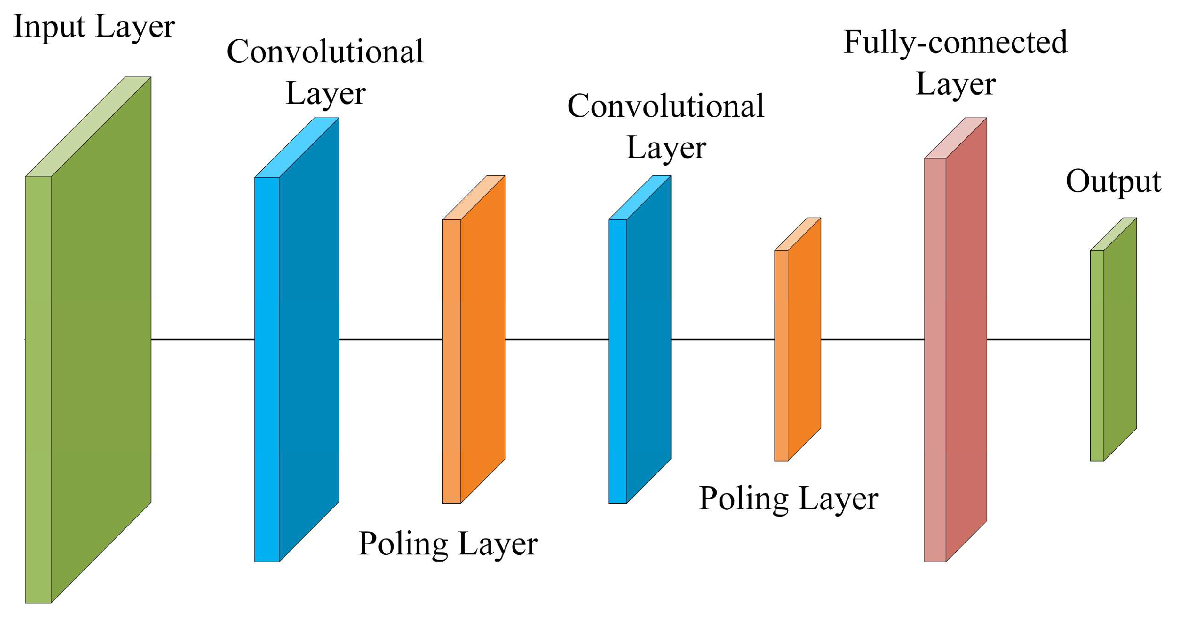
Figure 2.
GRU gating mechanism.
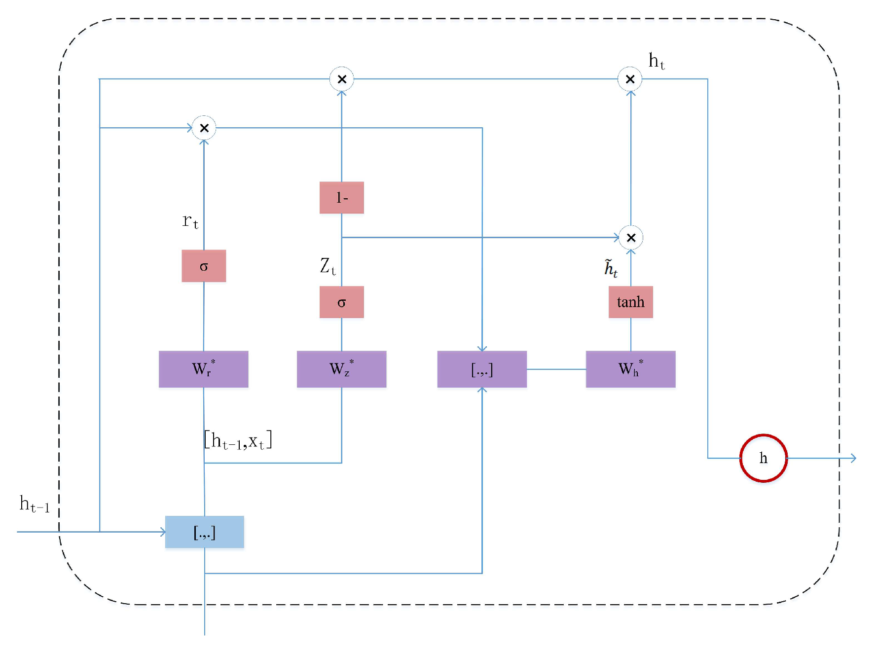
Figure 3.
Block structure diagram.
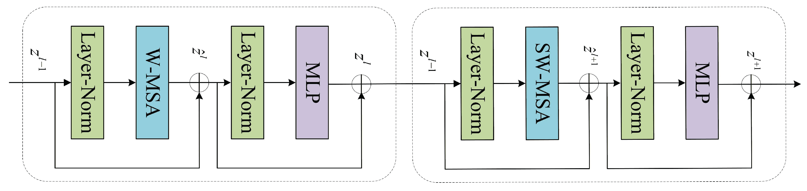
Figure 4.
Multi-Head Self-Attention diagram.
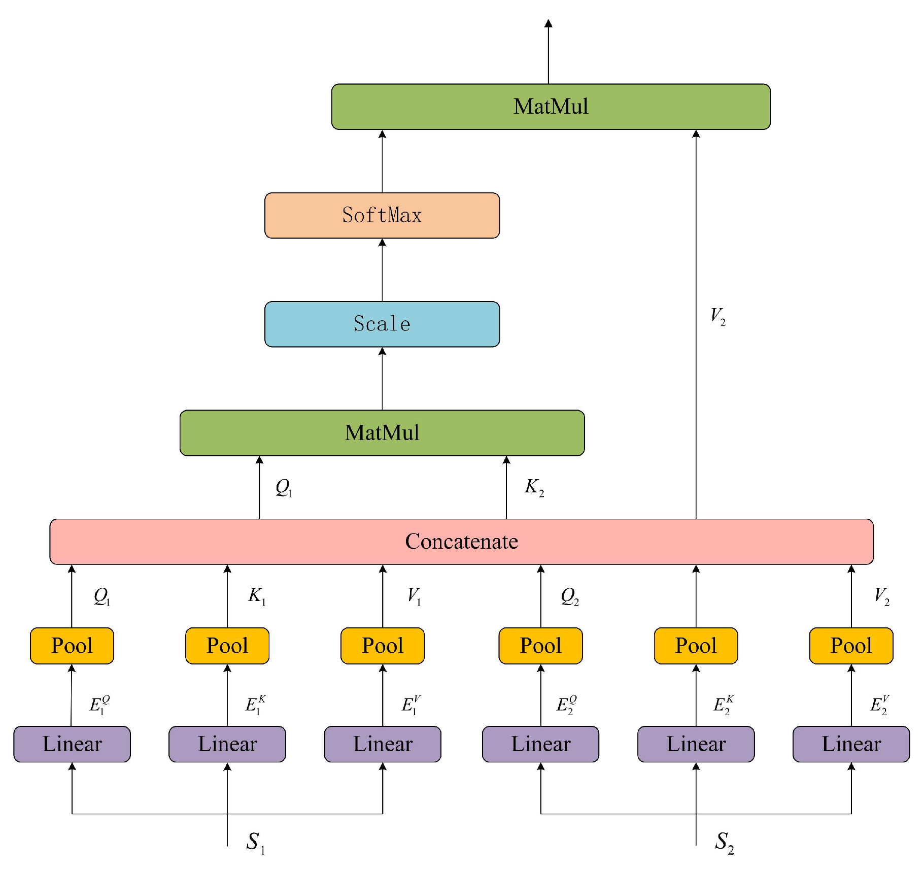
Figure 5.
CBAM.
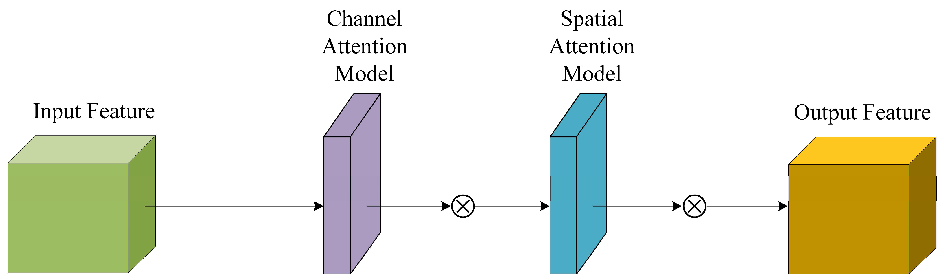
Figure 6.
Channel Attention Model.
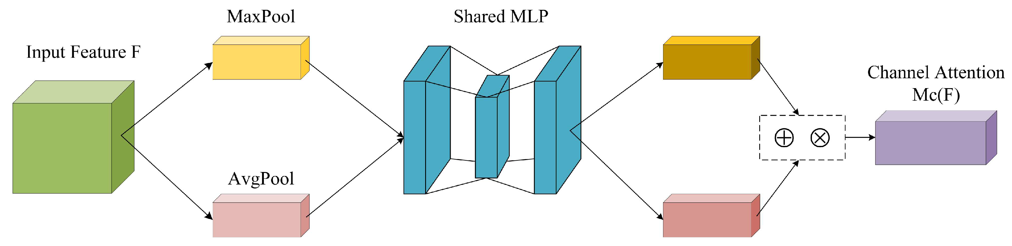
Figure 7.
Space Attention Model.
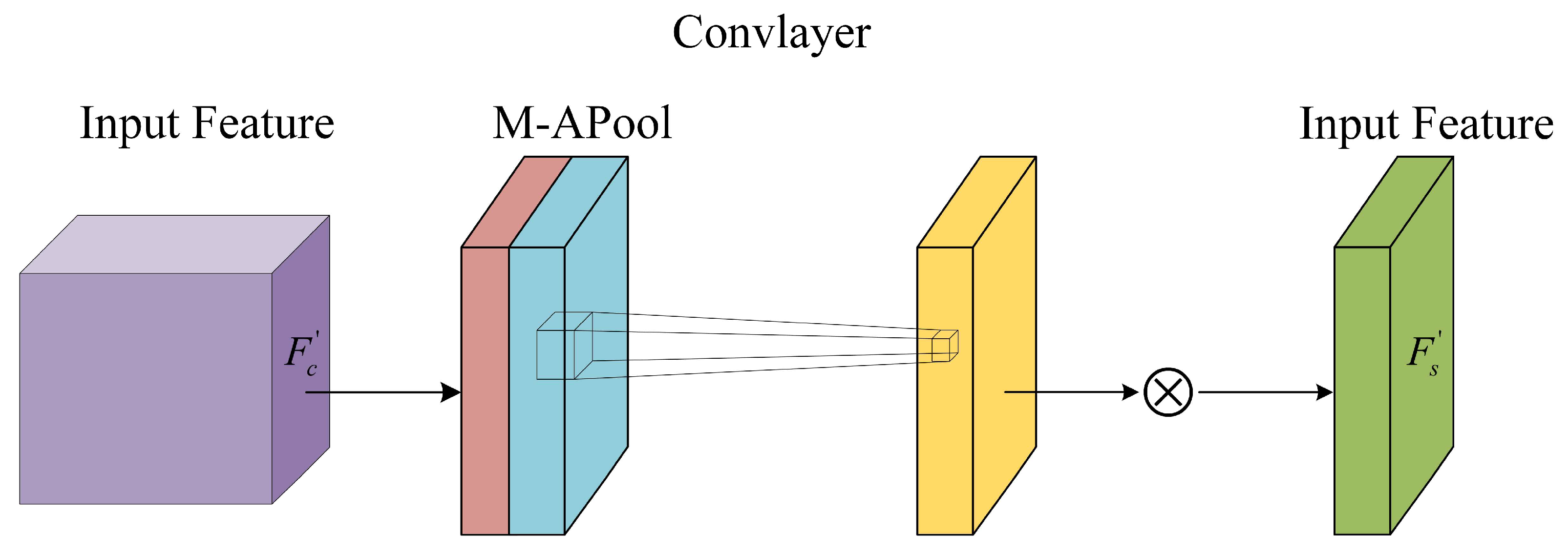
Figure 9.
AE Structural Diagram.
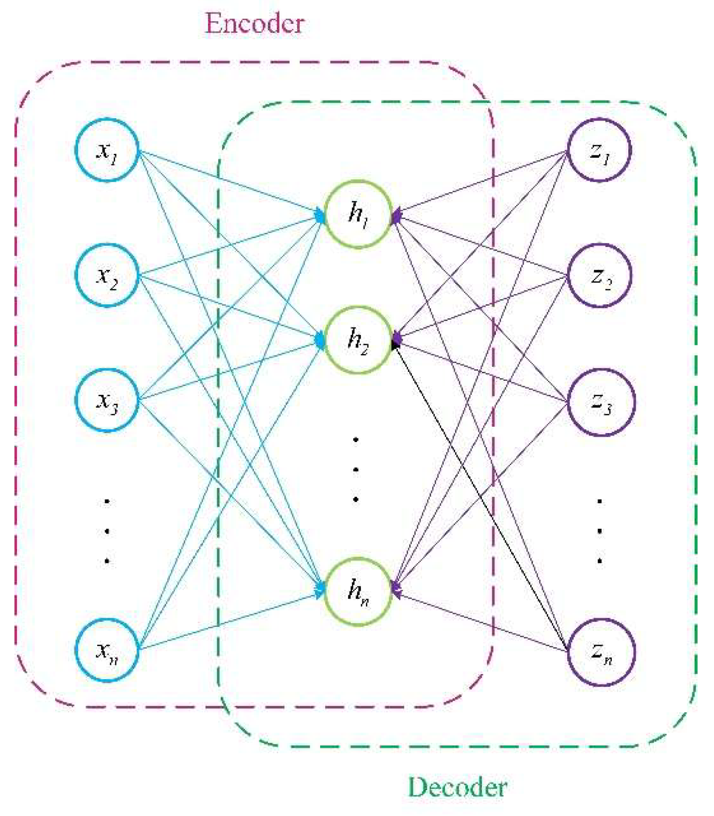
Figure 10.
Model.

Figure 11.
CAE Structural Diagram.
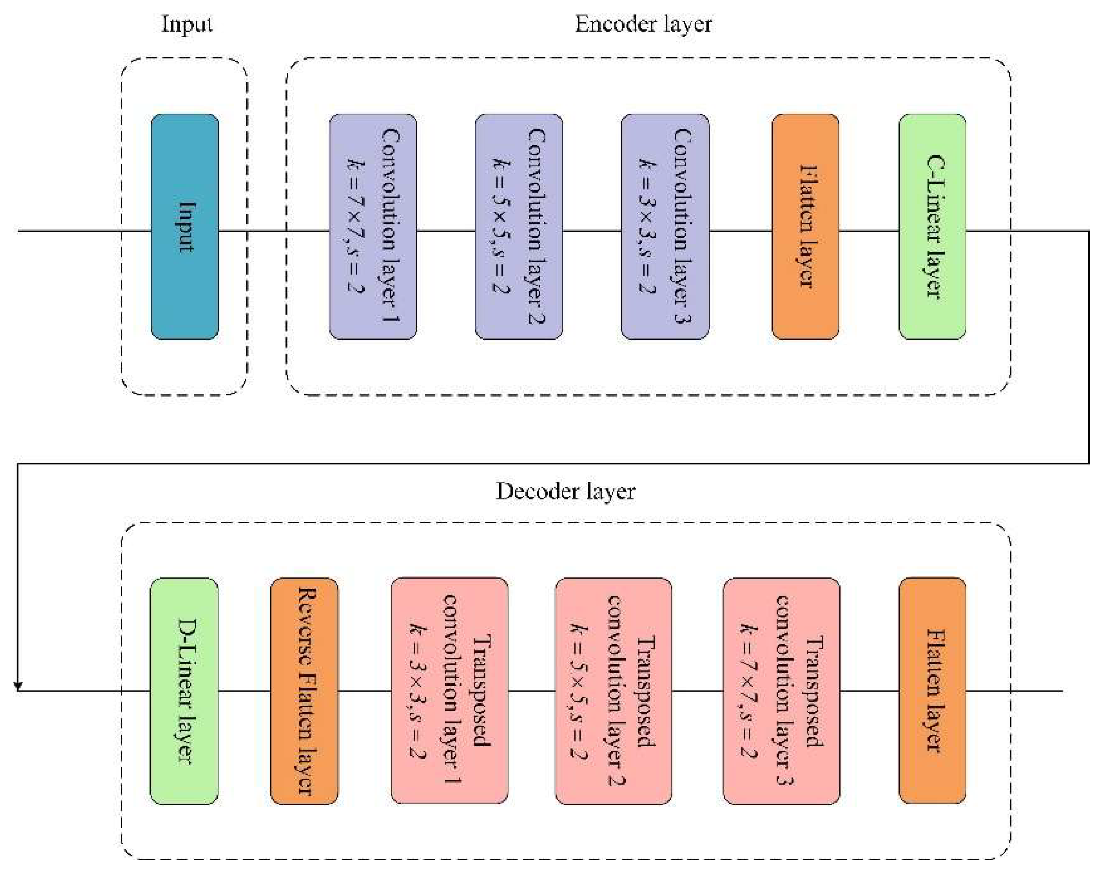
Figure 14.
Wavelet Transform Comparison Diagram.
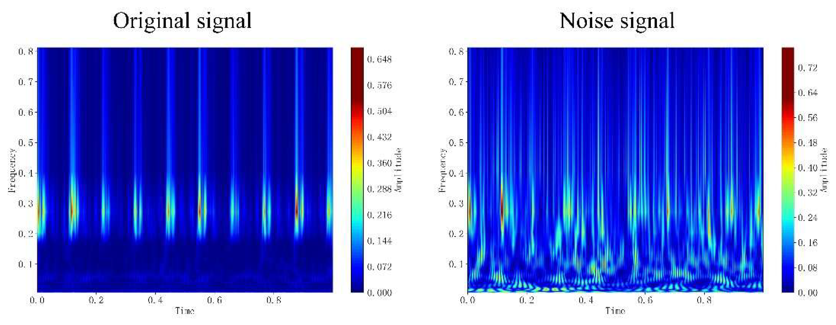
Figure 15.
Signal Envelope Comparison.
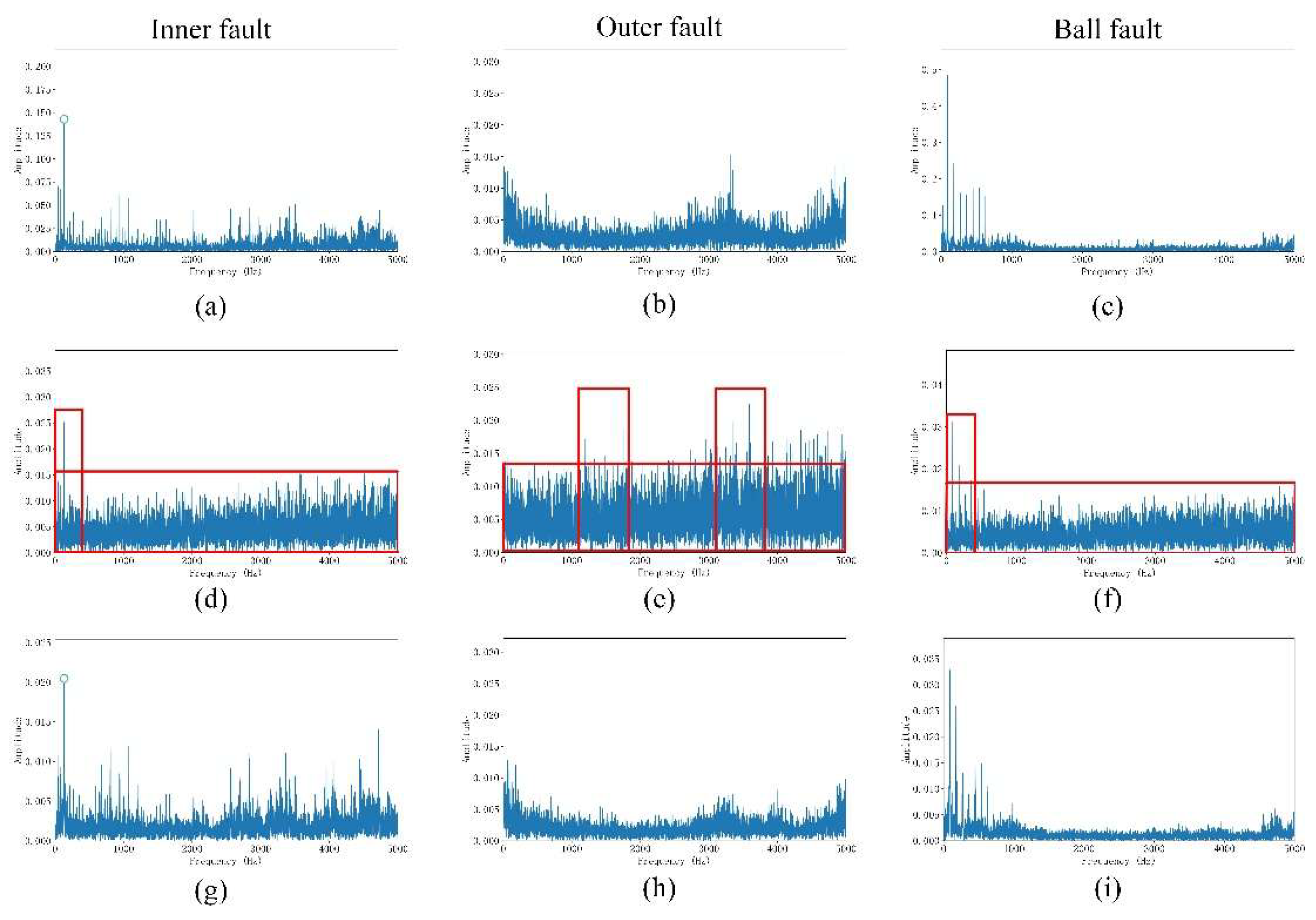
Figure 16.
MSE metric.
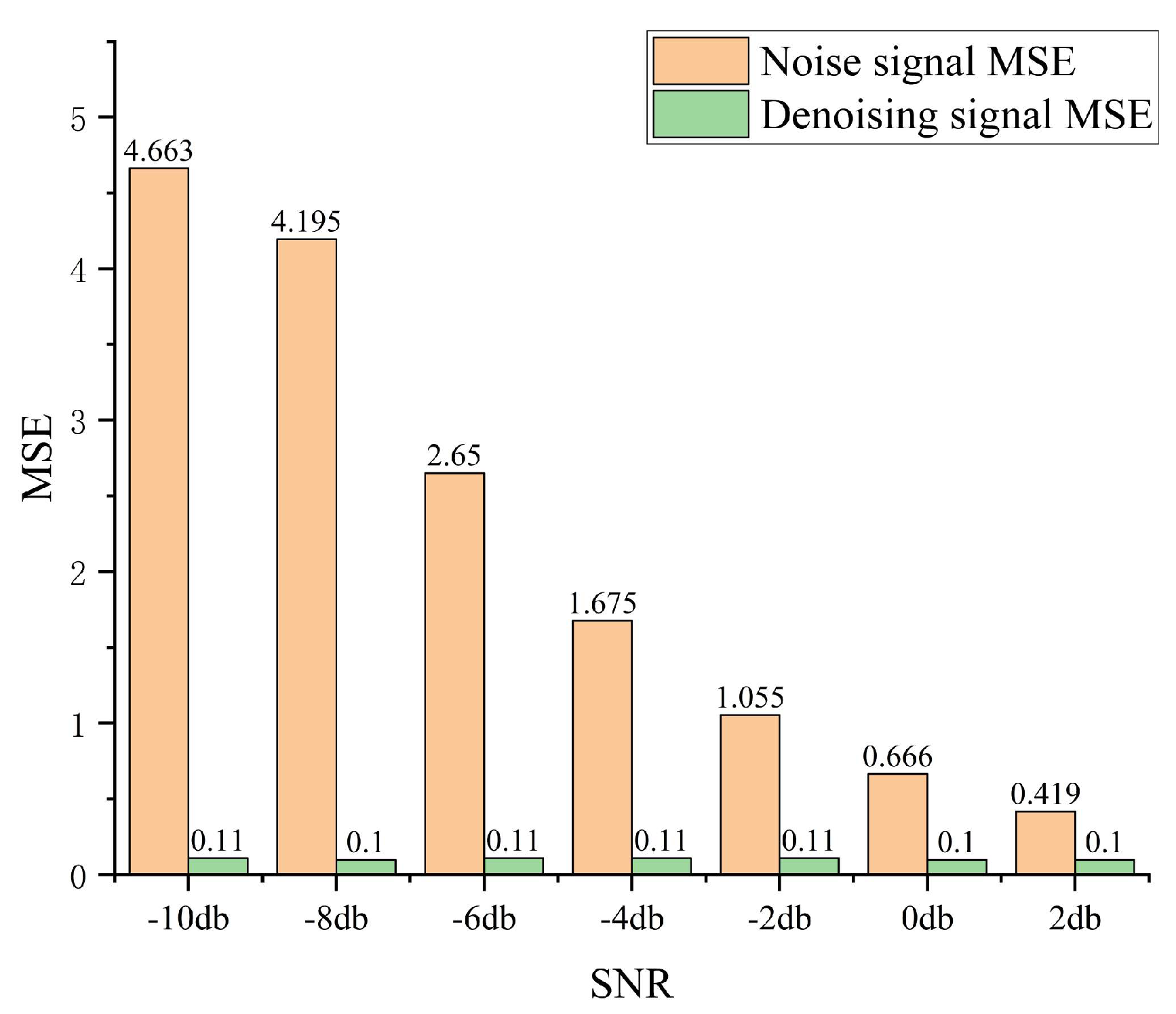
Figure 17.
CWRU Confusion Matrix.
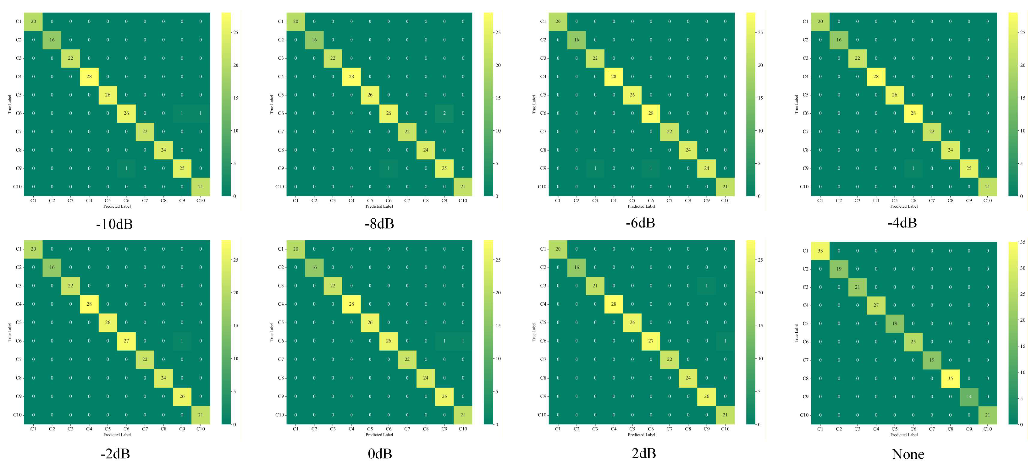
Figure 18.
CWRU T-SNE.
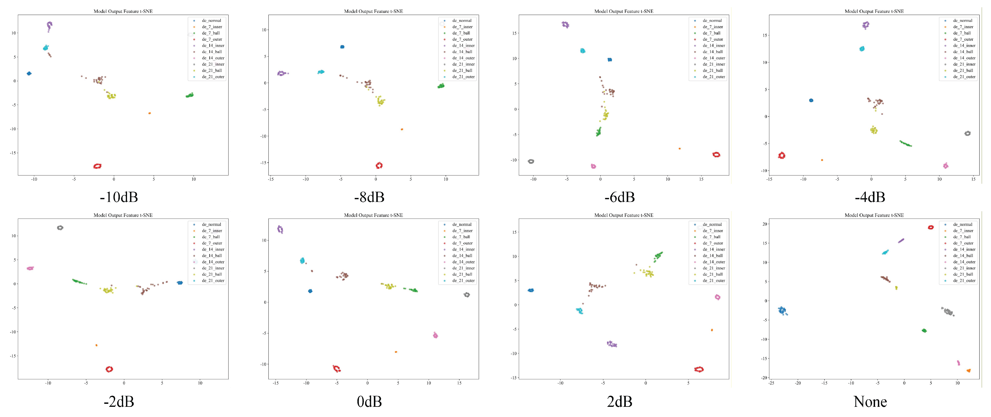
Figure 19.
Confusion Matrix.
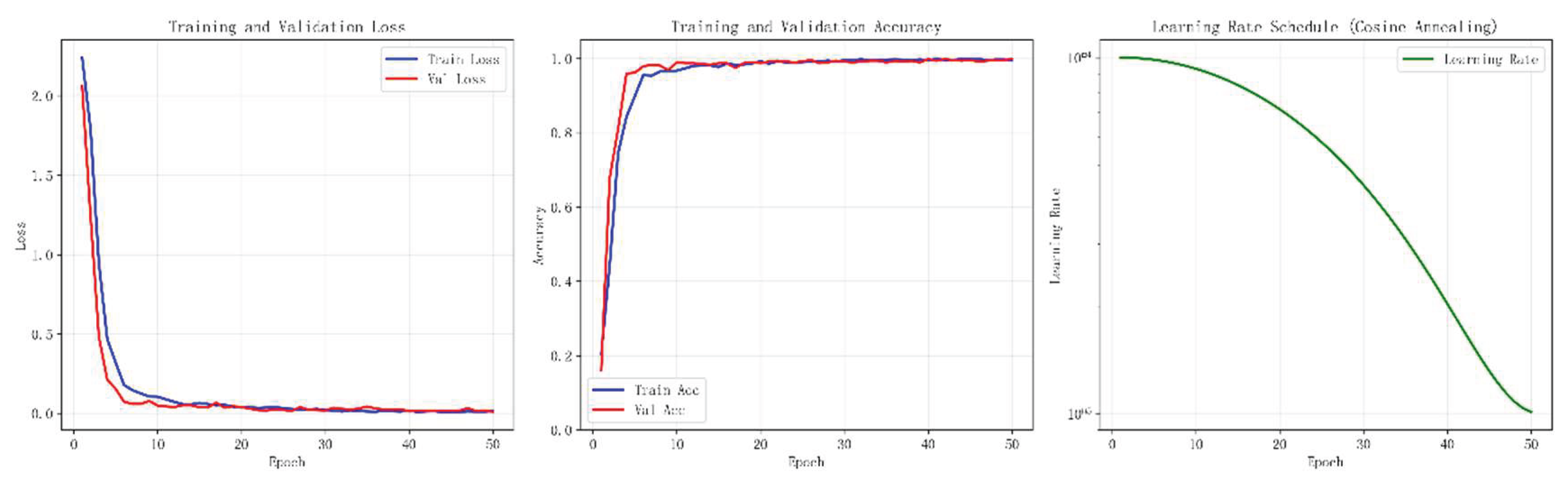
Figure 20.
Accuracy of Comparative Tests.

Figure 21.
-4dB Training Curve.

Figure 22.
Confusion matrix.
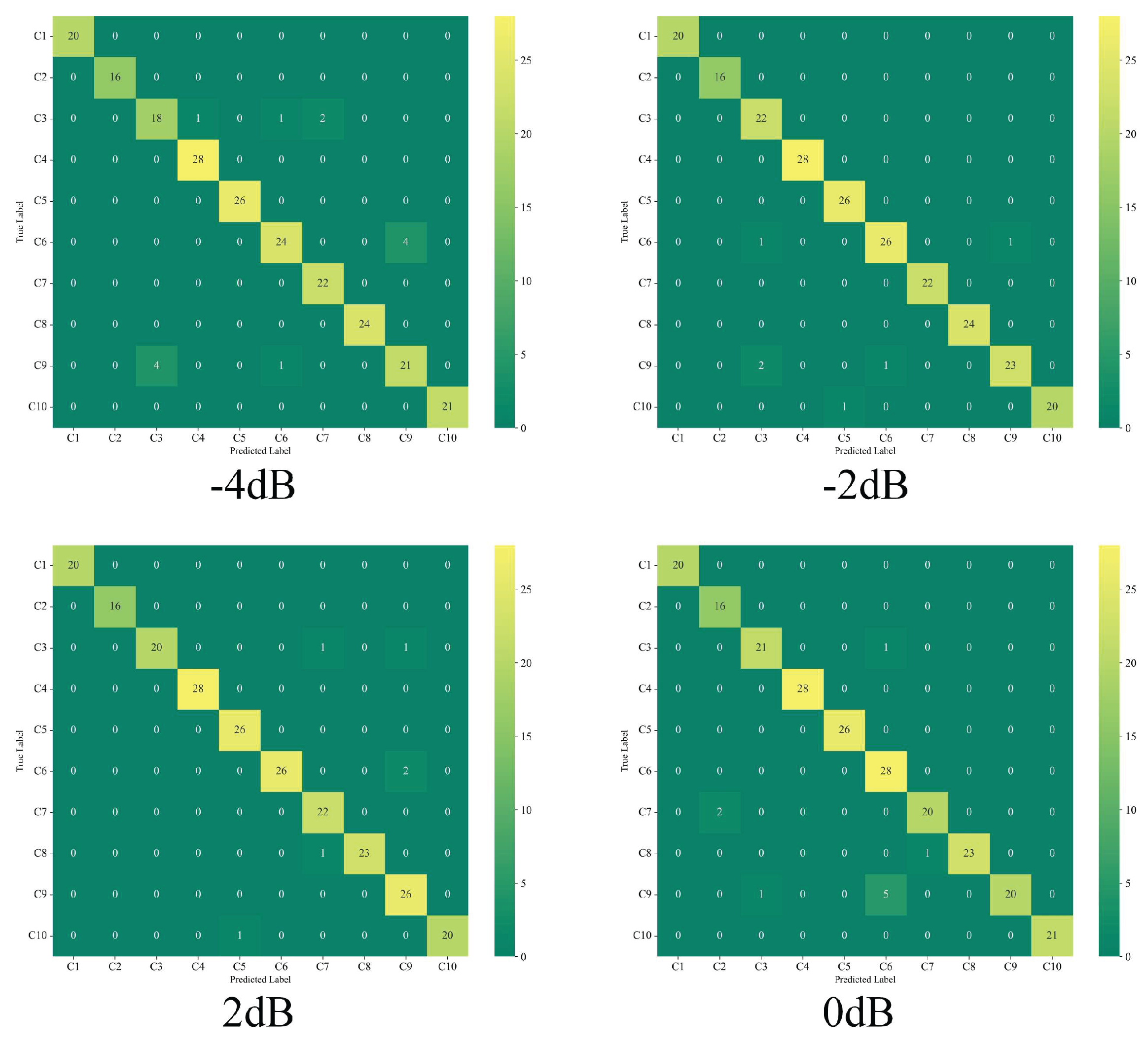
Figure 23.
Confusion matrix.
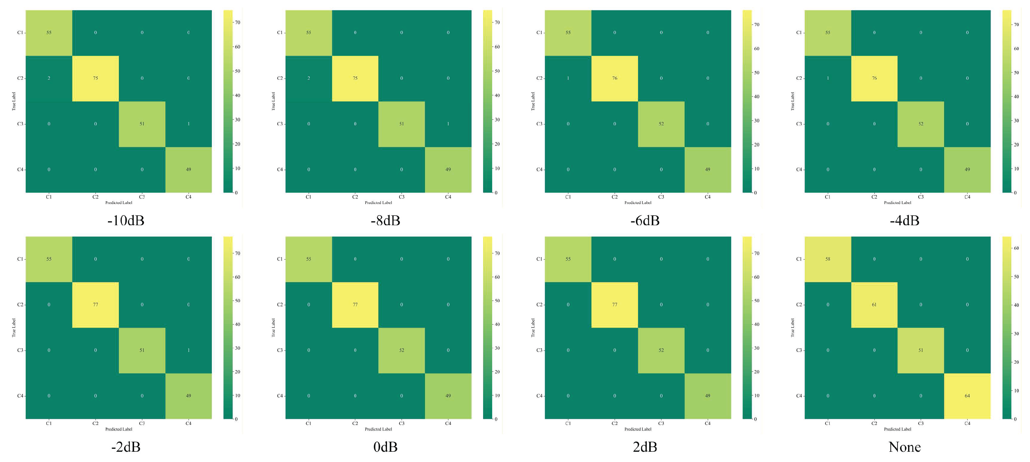
Figure 24.
Bearing test bench.
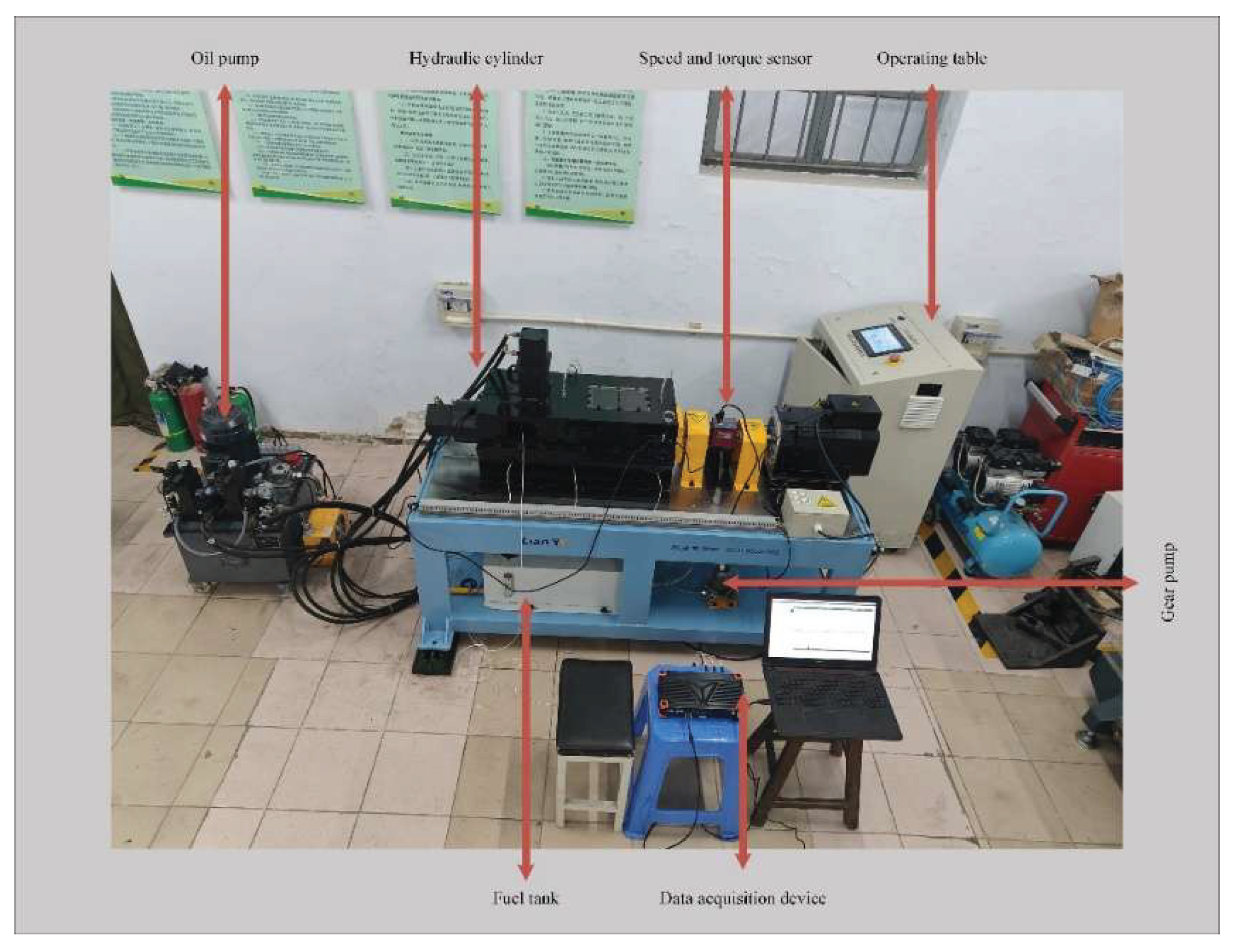
Figure 25.
Confusion matrix.
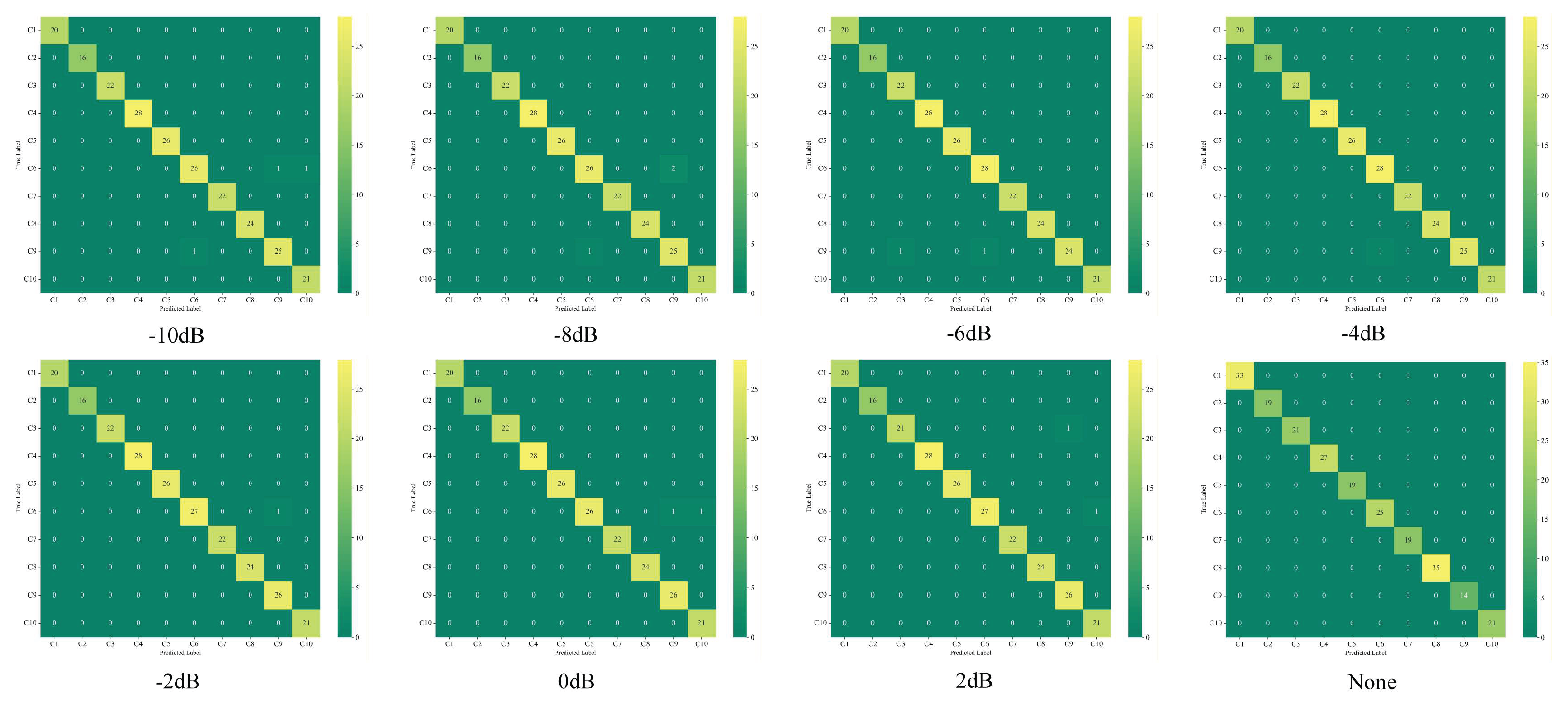
Figure 26.
Convolution Layer Weight Visualization.
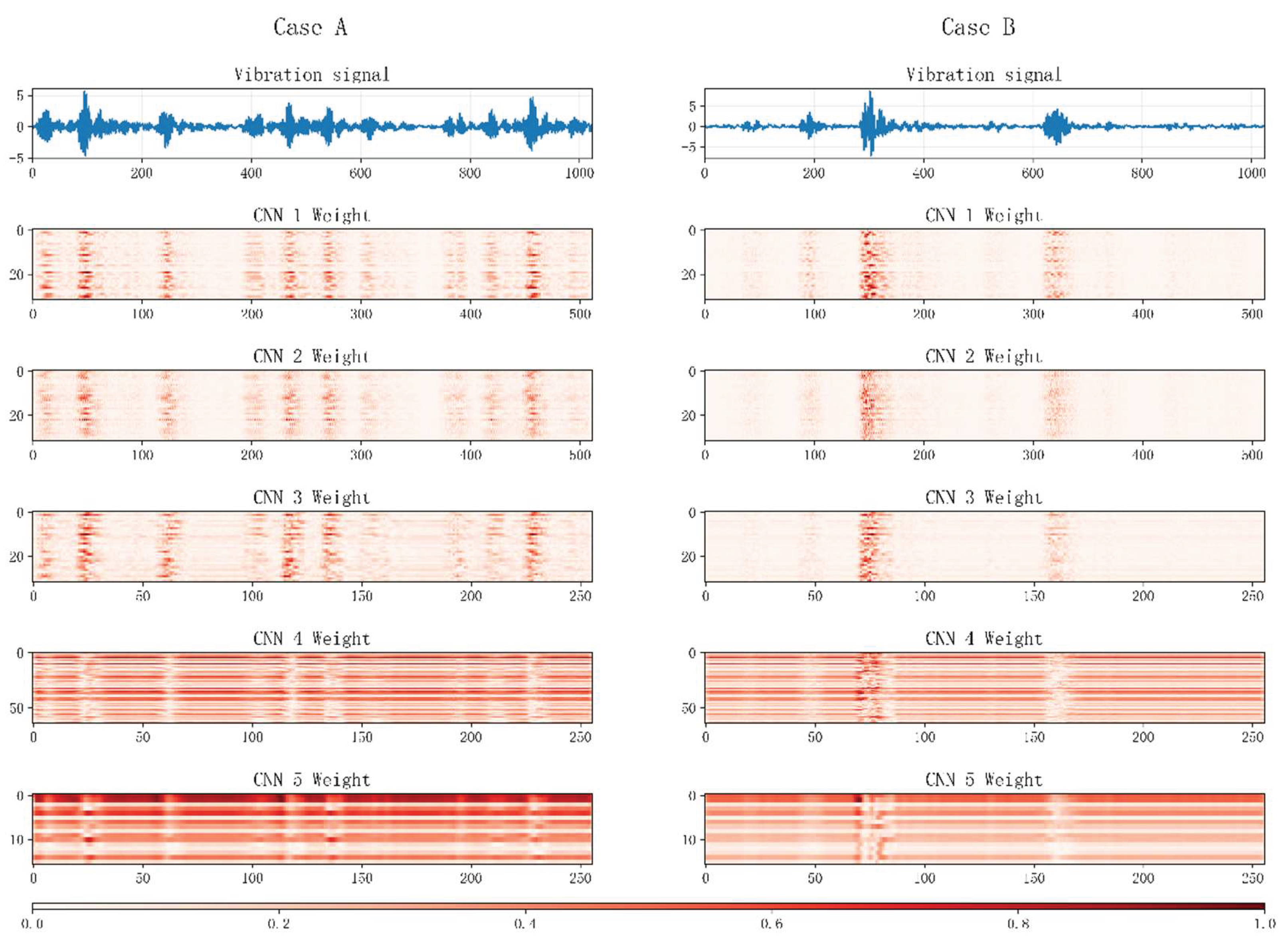

Table 1.
Module Parameter List.
| Module | Kernel size | Stride | Input | Output |
| Frequency domain | — | — | — | — |
| CNN0 | 7-7 | 2 | 3 | 32 |
| Res-Block1 | 7-7 | 1 | 64 | 64 |
| Res-Block2 | 7-7 | 1 | 64 | 64 |
| Res-Block3 | 7-7 | 1 | 64 | 64 |
| Conv1-1 | 1-1 | 1 | 64 | 128 |
| (S)W-Attention | 4-4 | 1 | 64 | 64 |
| Res-Block4 | 7-7 | 1 | 64 | 64 |
| Res-Block5 | 5-5 | 1 | 64 | 64 |
| Res-Block6 | 5-5 | 1 | 64 | 64 |
| Res-Block7 | 5-5 | 1 | 64 | 64 |
| Res-Block8 | 5-5 | 1 | 64 | 64 |
| Conv1-1 | 1-1 | 1 | 64 | 128 |
Table 2.
Module Parameter List.
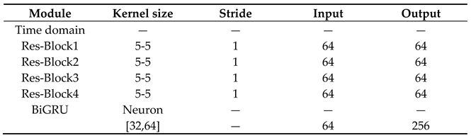
Table 3.
Image feature extraction.
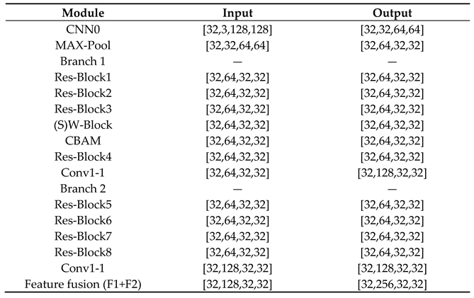
Table 4.
Vibration signal feature extraction.
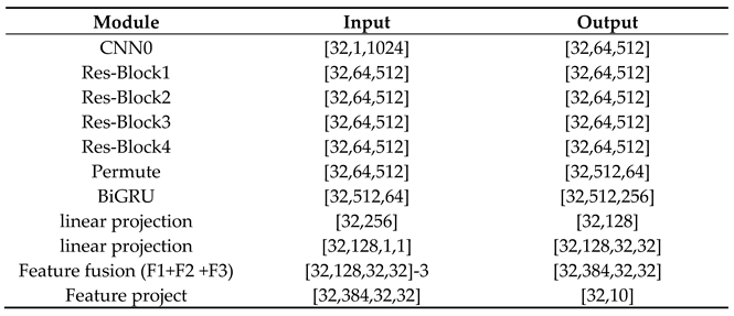
Table 5.
Introduction to the CWRU dataset.
| RPM | State of health | Fault diameter | Sample count | Tag |
| Normal | None | 233 | 0 | |
| 1797rpm | Inner | 0.007 | 233 | 1 |
| 0.014 | 233 | 2 | ||
| 0.021 | 233 | 3 | ||
| Ball | 0.007 | 233 | 4 | |
| 0.014 | 233 | 5 | ||
| 0.021 | 233 | 6 | ||
| Outer | 0.007 | 233 | 7 | |
| 0.014 | 233 | 8 | ||
| 0.021 | 233 | 9 |
Table 6.
Assessment indicators.
| SNR | Accuracy (Avg) |
Recall (Avg) |
F1-score (Avg) |
Precision (Avg) |
| -10dB | 93.99% | 94.20% | 94.24% | 94.52% |
| -8dB | 95.71% | 95.93% | 95.89% | 95.98% |
| -6dB | 96.57% | 96.76% | 96.68% | 96.69% |
| -4dB | 98.28% | 98.33% | 98.33% | 98.38% |
| -2dB | 98.71% | 98.78% | 98.73% | 98.74% |
| 0dB | ||||
| 2dB | ||||
| None | 100% | 100% | 100% | 100% |
Table 7.
CWRU model comparison table.
| Model | Accuracy (Avg) | |
| CNN-LSTM | a | 99.48% |
| KANTransformer | b | 99.07% |
| EWSNet | c | 83.88% |
| DCA-BiGRU | d | 84.40% |
Table 8.
Diagnostic results without using the AE model noise.
| SNR | Accuracy | Recall | F1-score | Precision |
|---|---|---|---|---|
| -4dB | 94.42% | 94.83% | 94.70% | 94.63% |
| -2dB | 95.71% | 95.91% | 95.77% | 96.19% |
| 0dB | 97.42% | 97.66% | 97.58% | 97.64% |
| 2dB | 97.42% | 97.48% | 97.53% | 97.76% |
Table 9.
Ablation Experiment Model.
| Model | Description | ||
|---|---|---|---|
| Model-1 | a | CNN+Windows-Attention+CBAM-7 | |
| Model-2 | b | CNN+Windows-Attention+CBAM-5 | |
| Model-3 | c | CNN+BiGRU | |
| Model-4 | CNN+Windows-Attention+CBAM-ALL | ||
| Model-5 | d | CNN-CBAM | |
| Model-6 | e | CNN-Windows-Attention | |
| Proposed Model | f | CNN+BiGRU-Windows-Attention+CBAM | |
Table 10.
Melting Model Evaluation Metrics.
| Model | Accuracy (Avg) |
Recall (Avg) |
F1-score (Avg) |
Precision (Avg) |
|
|---|---|---|---|---|---|
| Model-1 | a | 91.85% | 92.18% | 92.18% | 92.94% |
| Model-2 | b | 82.83% | 83.33% | 83.43% | 84.37% |
| Model-3 | c | 79.40% | 79.99% | 80.22% | 83.35% |
| Model-4 | d | 93.56% | 93.80% | 93.78% | 94.34% |
| Model-5 | e | 91.85% | 92.29% | 92.12% | 92.40% |
| Proposed Model | f | 93.99% | 94.20% | 94.24% | 94.52% |
Table 11.
Presentation of the simulation experiment data set.
| R. | State of health | Sample count | Tag |
|---|---|---|---|
| 1500rpm | Normal | 234 | 0 |
| Inner | 234 | 1 | |
| Ball | 234 | 2 | |
| Outer | 234 | 3 |
Table 12.
Evaluation Indicators.
| SNR | Accuracy (Avg) |
Recall (Avg) |
F1-score (Avg) |
Precision (Avg) |
|---|---|---|---|---|
| -10dB | 89.70% | 90.18% | 90.03% | 90.20% |
| -8dB | 94.42% | 94.49% | 94.57% | 94.69% |
| -6dB | 95.71% | 95.90% | 95.84% | 95.80% |
| -4dB | 97.85% | 98.03% | 97.88% | 97.79% |
| -2dB | ||||
| 0dB | ||||
| 2dB | 99.14% | 99.18% | 99.17% | 99.16 |
| None | 100% | 100% | 100% | 100% |
Table 13.
Image Signal Branch Parameters.
| Module | Dimension/kernel | Parameter |
|---|---|---|
| Image branch | — | — |
| CNN0 | in=3, out=32, kernel=7 | 9408 |
| Res-Block1 | in=32, out=64, kernel=7 | 73984 |
| Res-Block2 | in=64, out=64, kernel=7 | 73984 |
| Res-Block3 | in=66, out=64, kernel=7 | 73984 |
| Res-Block4 | in=64, out=32, kernel=7 | 73984 |
| (S)W-Attention | in=64, out=64, window=4 | 50033 |
| CBAM | in=64, out=64 | 678 |
| Res-Block5 | in=64, out=64, kernel=5 | 205056 |
| Res-Block6 | in=64, out=64, kernel=5 | 205056 |
| Res-Block7 | in=64, out=64, kernel=5 | 205056 |
| Res-Block8 | in=64, out=64, kernel=5 | 205056 |
Table 14.
Parameters of Vibration Signal Branch.
| Module | Dimension/kernel | Parameter |
|---|---|---|
| CNN0 | in=1, out=32, kernel=5 | 9408 |
| Res-Block1 | in=64, out=64, kernel=5 | 24832 |
| Res-Block2 | in=64, out=64, kernel=5 | 24832 |
| Res-Block3 | in=64, out=64, kernel=5 | 24832 |
| Res-Block4 | in=64, out=64, kernel=5 | 24832 |
| BiGRU | in=64, out=256, N= [32,64] | 445440 |
| Total number of parameters | — | 1730455 |
Table 15.
Model run times.
| Model/epochs | Time/s |
|---|---|
| 1 | 6.8 |
| 50 | 340.42 |
Disclaimer/Publisher’s Note: The statements, opinions and data contained in all publications are solely those of the individual author(s) and contributor(s) and not of MDPI and/or the editor(s). MDPI and/or the editor(s) disclaim responsibility for any injury to people or property resulting from any ideas, methods, instructions or products referred to in the content. |
© 2026 by the authors. Licensee MDPI, Basel, Switzerland. This article is an open access article distributed under the terms and conditions of the Creative Commons Attribution (CC BY) license.
Copyright: This open access article is published under a Creative Commons CC BY 4.0 license, which permit the free download, distribution, and reuse, provided that the author and preprint are cited in any reuse.


