
Submitted:
13 January 2026
Posted:
14 January 2026
You are already at the latest version
Abstract
This paper explores the link between economic performance and multidimensional well-being in the Italian context using a combination of the ISTAT BES approach (Benessere Equo e Sostenibile) and machine learning and clustering analysis. On the basis of a dataset of 19 Italian regions and the Autonomous Provinces of Trento and Bolzano from 2012 to 2023, it will be examined how the three BES components—Benessere (B), Equità (E), and Sostenibilità (S)—are intertwined with the Gross Domestic Product of the regions. Regarding the Benessere (B) component of well-being, the Gross Domestic Product will be analyzed using a regression approach of the K-Nearest Neighbors type to reveal the complex linkages between health outcomes, education outcomes, working conditions, social participation, and economic performance. The clustering of the B indicators and the Gross Domestic Product will be done using Hierarchical Clustering analysis to identify homogeneous territories characterized by different levels of quality of life and economic prosperity. Regarding the Equità (E) component of well-being, the regression analysis will be done using the Boosting algorithm to model the linkages between the Gross Domestic Product and the indicators of income distribution, poverty, material deprivation, and inclusion in the labor market. Boosting regression analysis will be particularly useful for this purpose since it models the complex interactions and thresholds of social and economic inequalities. Hierarchical Clustering analysis will be applied to identify the territories characterized by different levels of equity and economic growth. Regarding the Sostenibilità (S) component of well-being, the Gross Domestic Product will be modeled using Boosting regression analysis to reveal the very complex linkages between the economic performance of the territories and the indicators of environmental quality, risk of climate change, innovation outcomes, and the quality of public services. For this purpose, the analysis will use the Random Forest algorithm to identify the territories characterized by different levels of sustainability and economic performance. The analysis will show that the BES approach provides a very useful framework to identify the very different levels of linkages between the economic performance of the territories and the outcomes of the BES approach. The analysis will provide evidence that the BES approach is a very useful framework for the analysis of the linkages between the economic performance of the territories and the outcomes of the BES approach.
Keywords:
GDP
; BES
; sustainability
; regional inequality
; machine learning
1. Introduction
For decades, Gross Domestic Product (GDP) has been the dominant indicator used to measure economic performance and social progress. Yet, the limitations of GDP as a proxy for development are now widely acknowledged. GDP captures the monetary value of production but remains blind to fundamental aspects of social well-being, environmental quality, institutional strength, and equity. Regions can grow while becoming more unequal, environmentally degraded, socially fragmented, or unsafe. This disconnect has become increasingly evident in advanced economies, where economic growth no longer guarantees improvements in quality of life, social cohesion, or sustainability.
In light of these constraints, new development frameworks have been developed. Among these, ISTAT’s Italian Benessere Equo e Sostenibile (BES) framework is one of the most innovative methods developed to measure well-being in its multidimensional form. BES takes into account factors like health, education, security, work, income, social relations, institutions, environment, innovation, and public services to offer an inclusive vision of true living conditions. However, despite its high conceptual complexity, its empirical implementation within economic analysis is relatively limited. One of the core questions that are yet to be fully answered is whether or not the different aspects of well-being as measured through BES are mere reflections of social realities or whether they are capable of shaping economic performance. This thesis tackles this question by focusing on the relationship between BES factors and GDP in Italy. Contrary to traditional analysis that focuses on GDP and well-being as two distinct or rival aspects, this thesis takes a structural approach to understand well-being as an input within production. Thus, its core question is as follows:
To what extent are the multidimensional aspects of well-being, as measured through its different aspects of Benessere, Equità, and Sostenibilità, able to influence economic performance in Italy, and to what extent can these relationships differ across territories?
This is an extremely pertinent question within an Italian setting that is marked by high levels of disparities in different aspects like income, health, security, public services, infrastructure, education, and environmental quality. Northern territories and self-governing regions are generally known to have high levels of GDP, as well as high levels of quality in terms of infrastructure and institutions, whereas southern territories are known to experience problems in terms of infrastructure, high crime rates, social capital, and environmental vulnerability. It is therefore necessary to establish whether or not these are mere co-variables to GDP or whether they are structurally responsible for it in order to make informed decisions about development.
The literature on regional growth and development can be broadly classified into three strands. The first strand deals with traditional factors such as capital accumulation, human capital, innovation, and agglomeration. The second strand deals with social and institutional factors such as crime, trust, governance, and inequality. The third strand deals with environment and climate change risks. While each of these strands provides important and useful results, they examine these aspects in a disconnected manner. What has been largely missing in the literature is an integrated framework combining these aspects of economic performance, social welfare, equity, and sustainability in a unified empirical model. Furthermore, few studies in the literature use BES per se, despite its richness and relevance in the Italian context. Most empirical studies based on BES use it in a descriptive manner, in terms of rankings and composite indices rather than their relationship with economic performance in a causative and structural manner. In addition, the traditional literature in econometrics has largely followed a linear or log-linear model, implying strong functional form restrictions and a lack of suitability in capturing nonlinear and threshold-based relationships and regional heterogeneities in regional systems. For example, the relationship between the economy and crime, public transportation, health, and environment awareness can be nonlinear in the sense that it depends on whether a region lies on the left or right side of certain development thresholds, and these aspects remain obscured in traditional regression analysis. This paper fills these research gaps in three basic ways. Firstly, the indicators of BES are conceived not as outcomes but as drivers of GDP, with well-being treated as an input into the production of regional income. The security, health, education, environmental, and social inclusion aspects of well-being are conceived here as productive assets that influence investment, labor, innovation, and competitiveness. Secondly, a new methodological approach is developed that brings together panel econometrics, regression analysis using machine learning, and clustering in a unified framework that allows the analysis to explore causal linkages in time and complex geographical patterns in a unified way. Finally, this research will carefully distinguish between the three-pillar structure of BES, Benessere (B), Equità (E), and Sostenibilità (S), in contrast to using a single indicator that summarizes all three, so that we can determine which aspects of well-being count the most for GDP. These regional economies are complex adaptive systems that involve feedback, complementarities, geographical spillovers, and non-linear dynamics. For instance, raising public transport by a marginal amount would have little effect in an unconnected rural region but would have a dramatic effect in an urban region plagued by congestion; and awareness of climate change would trigger innovation only in regions that have some research capacity already. Linear models cannot handle such dynamics. This research, therefore, uses machine learning models suited to each BES dimension. In Benessere, GDP is modeled using K-Nearest Neighbors (KNN) to reflect similarities and differences in how health, safety, and services matter to different regions' income. In Equità, GDP is modeled using Boosting, which is good at detecting inequality thresholds and non-linear effects of inequality. In Sostenibilità, again in GDP, Boosting is used to model non-linear dynamics of environmental risk, awareness of climate change, and innovation. This is an original contribution since instead of trying to find “best” models, it recognizes that different socio-economic systems have different data-generating processes. But in addition to this, the analysis applies clustering to identify regional development paths. For Benessere and Equità, Hierarchical Clustering is used, and regions with similar values of GDP, health, safety, inclusion, and social capital are clustered. For Sostenibilità, regions are clustered using the Random Forest algorithm, and the complex relationship between environmental quality, innovation, and infrastructure is captured. The analysis identifies regions on virtuous paths, where economic, innovation, and sustainability outcomes feed each other, and others on paths of cumulative disadvantage, where low GDP, poor public services, and social vulnerability trap each other. The originality of this work consists in its comprehensive concept of development. Instead of focusing on whether there is a relationship between GDP and well-being, or on whether there is a connection between them, this work asks whether well-being generates GDP. Moreover, while other studies rely on a single statistical tool, this work relies on a variety of machine learning and clustering techniques, each one chosen according to the specific characteristics of the dimension of the BES being analyzed. In this manner, three main results are obtained. Firstly, there is empirical evidence that well-being, equity, and sustainability are not a luxury that only rich areas enjoy but are actually structural factors influencing economic performance. Secondly, there is evidence that there are multiple development regimes within the Italian regional system, contrary to a simple North-South dichotomy. Thirdly, there is evidence that machine learning techniques are not only predictive tools but a strong analytical instrument for economics, able to discover hidden patterns within socio-economic systems. By including GDP within the BES paradigm, this work presents a new vision on growth: growth not only as an autonomous economic process but as a process that naturally derives from a set of social, institutional, and environmental systems working well—or failing to work well together.
2. Literature Review
The current literature agrees on a key assertion: economic growth must be studied in relation to social welfare, institutions, and sustainability. This view is in line with the BES (BES) model and the sustainability-driven economic growth model presented in this study. Ahammed et al. (2025) have found that blue economy factors such as ocean resources, protection of the environment, and coastal innovations contribute substantially to economic growth in China, thus verifying the productive role of natural capital in relation to proper engagement with institutions and innovations. The same results are found in the studies of Berberoglu et al. (2024) and Chengliang et al. (2025), which found that environmental policies and sustainable use of resources are facilitators rather than inhibitors of economic performance. Additionally, Du et al. (2024) have found energy security to have an effect on economic growth, thus emphasizing the importance of infrastructure reliability in achieving sustainable economic growth. The importance of human welfare, as an input in economic production, is also adequately argued. Anauati et al. (2025) measure economic costs related to poor sleep habits, while Barbier and Mensah (2025) prove that environmental risks to health have harmful impacts on economic development and human welfare. The complex linkages between health, environment, and economic development are also clarified in Dar et al. (2025), which uses machine learning to model non-linear dynamics in these linkages. Akinlo and Okunlola (2025) also highlight the importance of institutions in these linkages, arguing that economic freedom improves human welfare but in environments that are high in political risk, and that it is necessary to have state capacity to measure human welfare properly. Grashof (2025), and also Crozet et al. (2024), also argue that to measure human welfare and regional economic performance, one must move beyond income to structural-compositional analysis. Moreover, the views from the historical school and the degrowth school offered by Buscemi (2025) and Chakori et al. (2026), respectively, refute the assumption that economic growth is a necessary condition for prosperity and suggest that economic stability can be attained through redistribution, resilience, and social cohesion. Gylfason and Nganou (2025) illustrate that the development of Mongolia can be fueled by the use of mineral resources in the development of human and social capital. However, the findings in Haroon and Hayyat (2025) suggest that the economic development in regions caused by mining is subject to environmental strain. The role of the environmental channel is evident in the fact that the primary role of critical minerals in the achievement of green growth is in the sustainable energy transition according to the findings in Hwang et al. (2024). Also, the findings in Insaidoo et al. (2025) show a significant decrease in the level of production in Africa caused by extreme weather conditions.
Lastly, the views in Infante-Amate et al. (2024) support the fact that the decoupling of well-being from emissions in the context of economic growth is a long-term reality. Le et al. (2024) suggest that the energy intensity of well-being increases in the absence of technological and institutional changes.
Well-being and life satisfaction positively affect economic performance, supported by the research of Hussien et al. (2025) and Iuga et al. (2025) in terms of health spending, which is a result of environmental quality and income, as found in the study of Islam and Baida (2025). These researches emphasize the need for social investment, which is not a cost but a driver for economic growth. Institutions and finances play a similarly crucial role in achieving sustainable growth, with Kunawotor et al. (2025) relating the role of the state’s size and quality of institutions in the performance of welfare in Africa and Martynenko et al. (2025) proving that fiscal decentralization increases sustainability in a region. The importance of digitalization in European economic growth is highlighted in the research of Lobonț et al. (2025) and Mashaqbeh (2025) in terms of the stabilizing effects of remittances in Jordan. In a collective manner, these researches reaffirm the need for alternative and post-growth theories that relate development, equity, and sustainability, supported by Lauer et al. (2025) and Levy (2025) in their research. The causal relationship between culture and economic and social performance in Europe is examined in the research of Mažeikaitė (2025) and indicates that values, norms, and trust influence economic performance in a productive manner, in accordance with the BES view that social capital and civic engagement play a decisive role in economic performance in a region. Territorial and geographical determinants also influence economic performance. According to Mikheeva (2025), geo-strategic location affects regional development in Russia, while Tan et al. (2025) indicate that tourism is a factor in human development and economic income in the ASEAN countries. Public engagement affects the economic performance of the region (Tleuberdinova et al., 2025), indicating that development is contingent upon public engagement in economic activities. Well-being and demographic determinants are also of great significance; hence, Mohamed et al. (2025) indicate a positive feedback loop between life expectancy and per capita GDP in Somalia, while Munawaroh et al. (2025) indicate that aging populations have significant macroeconomic impacts in Indonesia. These findings are supported by the views of Warner et al. (2025) who propose that an aging population requires a paradigm shift in the theory of growth economics, labor economics, and regional policy; this marks the beginning of the BES transition from quantity to quality of life. Distributional and multidimensional methods extend this paradigm. Natanael (2025) finds that commodity diversification improves equality and human development, and Okogun & Hiwatari (2024) define poverty as a multidimensional concept, especially in terms of women and children. Rijpma et al. (2025) find historical support for the superiority of composite development metrics in long-run development analysis compared with GDP. Sustainability and technology development are integral to these dynamics. Tian et al. (2024) find that social trade-offs accompany private mining sector investments in rural communities, and Tiwari et al. (2024) find mutual benefits of fintech and green finance. Utouh & Kitole (2025) emphasize the large social opportunity costs of massive infrastructure development. Wu et al. (2025) find that energy corporations' entry into countries with low environmental performance faces challenges in terms of legitimacy, hindering long-run development, and illustrate how institutional and environmental vulnerabilities impede economic performance. This confirms the BES hypothesis about the importance of environmental and institutional structure in economic performance, rather than considering them as externalities. Labor dynamics in the labor market and social stability are also important in energy transitions. Xolmurotov et al. (2025) demonstrate that an increase in the use of renewable energy sources decreases unemployment in Uzbekistan, implying that a green transition ensures inclusive growth. Zéman et al. (2025) further widen this focus to be global in coverage and demonstrate that material consumption behavior and energy structure are important in determining various dimensions of social and economic welfare outcomes. The human factor also plays an important role in transitions in any economy. Zhou et al. (2025) demonstrate that human capital and happiness are important in determining migration and economic growth in China and that labor mobility and productivity are subject to social and educational factors. Life expectancy and environmental sustainability are also important in BRICS countries in achieving inclusive growth in transitions, as asserted by Yeboah et al. in 2024, who further argue that the quality of growth is more important than the quantity of growth in transitions. See Table 1.
3. Methodology
The link between economic growth and well-being is, in itself, complex, multifaceted, and regionally specific. Social inclusion, environmental sustainability, innovation, public service, and trust in institutions do not affect GDP in a straightforward or cumulative fashion, but rather through complex interlinkages, feedback effects, thresholds, and cumulative processes. For this reason, this research employs a comprehensive research methodology that brings together panel econometrics, regression analysis using machine learning, and clustering analysis, which can support both causal analysis and the detection of underlying structural patterns. Specifically, panel econometric analysis will be used in this research for initial analysis, aiming to detect the typical dynamic link between GDP and the set of BES indicators. The need for this initial analysis stems from the fact that region-specific features, such as geographical, developmental, and institutional characteristics, tend to be constant and not easily observable, but still tend to significantly influence economic performance. The fixed effects model and the random effects model will be estimated in this research in order to account for these region-specific features and filter out the influence of changes in well-being for each region. The underlying question this research seeks to address is: "Can a better health, security, environmental, and social situation in a region be translated into increased economic growth, measured through higher GDP values, in the long run?" However, linear panel regression models imply very strong form constraints on the function and assume linearity in the effects of, for example, crime reduction, the promotion of renewable energy sources, and education on the dependent variable for all regions and levels of development. In reality, this linearity and homogeneity of effect do not exist in nonlinear and threshold phenomena in the regions’ systems. Hence, panel regression models are extended with machine learning algorithms. Machine learning algorithms are particularly well-suited to the detection of complex nonlinear interdependencies and relations common to socio-economic systems like the regions’ systems. In contrast to linear panel regression models that imply a strict form on the function to estimate and assume linearity in the effects of the variables on the dependent variable for all regions and levels of development, machine learning algorithms do not imply any structure on the function and instead allow the structure to emerge from the data itself on the interdependencies between the various dimensions of well-being and the GDP variable. The choice of the machine learning algorithms for the various dimensions of well-being depends on the algorithms’ forecast accuracy for the GDP variable for the regions’ systems. In the Benessere (B) dimension of well-being, the K-Nearest Neighbors machine learning algorithm will be applied due to its sensitivity to local similarities among the regions and the assumption that regions with similar social and health characteristics follow the same growth path for the GDP variable. In the Equità (E) and the Sostenibilità (S) well-being dimension of the regions’ systems, the This is an essential step, as well-being does not have a smooth and proportional impact on GDP, as, for instance, small increases in social inclusion might have a limited effect in developed areas but a strong effect in other areas. Machine learning makes it easier to detect these relationships. Regression analysis explains how well-being influences GDP, and the other part of the analysis, clustering, explains how regions are grouped in specific regimes of development. This is an essential part of the analysis since Italy has not one but many models of growth. Hierarchical clustering is employed on the Benessere and Equità dimensions since these variables are associated with deeply embedded social and institutional settings that develop in a very gradual and nested territorial way. However, for the Sostenibilità dimension, Random Forest Clustering is employed since the nonlinear relationships between environmental and innovation variables are very complex and result in specific sustainability and growth patterns, not easily detectable through other methods, like distance metrics. By combining panel econometrics, machine learning, and clustering, the analysis can go from simple correlations to a deeper interpretation of the results. Panel models detect causality in a temporal framework, while machine learning and clustering detect nonlinear and heterogeneous relationships and the presence of territorial regimes, respectively. This comprehensive approach is therefore crucial for comprehending how the BES dimensions not only measure social outcomes but are, in essence, prime drivers of Italian regional GDP performance.
Figure 1.
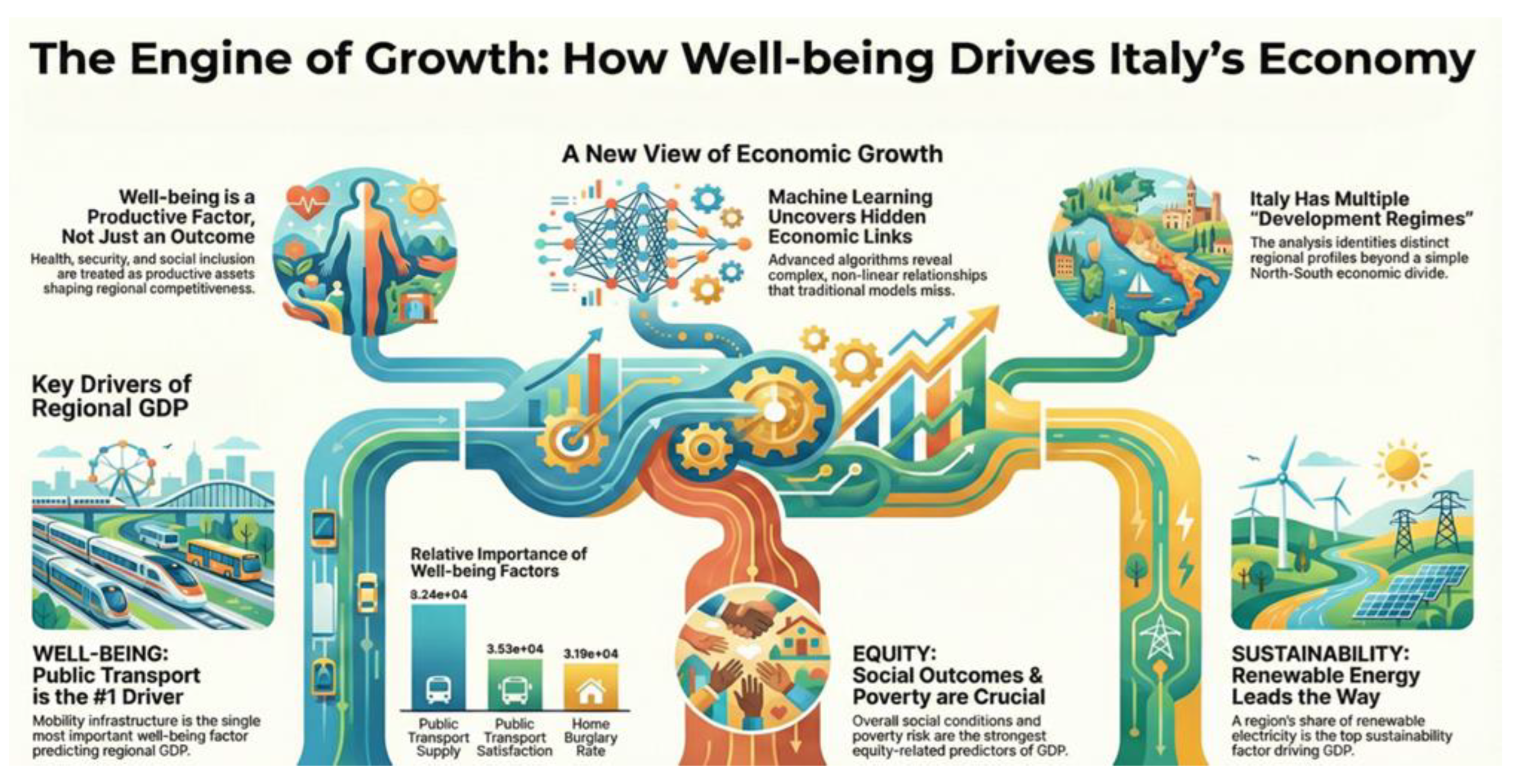
The Engine of Growth: How Well-Being, Equity, and Sustainability Drive Italy’s Regional Economy. This figure summarizes the BES-based analytical framework, showing how well-being, equity, and sustainability jointly shape regional GDP in Italy. Machine-learning and clustering results highlight nonlinear interactions and distinct territorial development regimes driven by mobility, social inclusion, innovation, and environmental quality.
Figure 1.
The Engine of Growth: How Well-Being, Equity, and Sustainability Drive Italy’s Regional Economy. This figure summarizes the BES-based analytical framework, showing how well-being, equity, and sustainability jointly shape regional GDP in Italy. Machine-learning and clustering results highlight nonlinear interactions and distinct territorial development regimes driven by mobility, social inclusion, innovation, and environmental quality.
4. From Quality of Life to Economic Output: The Benessere–GDP Nexus
This research focuses on the role of the B-Benessere (Well-being) component in the ISTAT-BES approach in influencing the GDP in Italy from 2012 to 2023. While recognizing the fact that economic development is inextricably linked with the determinants of well-being, the research considers personal security, the availability of basic services and health care as fundamental drivers of the quality of life that in turn affect aggregate economic performance. For a territory with a high degree of heterogeneity in Italy, the differences in the regions' well-being drivers are the source of disparities in economic performance. The research uses a panel data approach in 21 regions in Italy and defines GDP as a function of the crime rate, the availability of public transport services, and the density of the number of medical doctors. The primary research question is whether improvements in the regions' well-being are correlated with increases in the regions' economic output. With the inclusion of the GDP-Benessere variables in the research model, the research defines the drivers of the well-being in terms of the social outcomes of economic development. The research proposes an integrated approach to economic development in line with the BES approach. According to the research approach, economic performance and the quality of life are intertwined in a way that is not contradictory but mutually reinforcing. See Table 2.
Specifically we have estimated the following equation:
where i=21 and t=2012-2023.
The panel dataset estimates how regional GDP correlates with the first four main factors of well-being identified in the ISTAT-BES method: security, measured by rates of home burglary and robbery; access to collective services, measured by access to public transport; and healthcare, measured by the density of medical doctors. In a BES perspective, GDP is conceptualized not only as an end but also as an economic outcome that corresponds to the quality of social, institutional, and environmental factors. In this respect, this study tries to assess whether there is a structurally significant link between well-being and economic performance for Italian regions from 2012 to 2023. The Hausman test confirms that there is no correlation between unobserved regional variables and explanatory variables, suggesting that a fixed effect estimation is appropriate. This is not surprising, given that crime rates, healthcare systems, and transport networks are all affected by regional factors such as governance quality, path dependence, and social capital in Italy. As a consequence, fixed effect estimation is appropriate since it allows identification of how variations in well-being affect regional economic performance. The test on group intercepts additionally confirms that there is significant inter-regional variation. This has important methodological implications, especially from a BES perspective. In fact, well-being is a territorial concept since there are significant inter-regional variations not only with respect to income but also with respect to institutions, security, healthcare systems, and access to services. Omitting this structural characteristic would produce biased estimates on how GDP relates to BES indicators. The results show a significant, large, and negative impact of both crime variables, the burglary rate and robbery rate, on the regional GDP. This result indicates that there is a systematic association between high levels of crime and poor economic performance. In the BES framework, security is shown to be both a social asset and a productive input, since it increases transaction costs, deters investments, reduces tourist inflows, erodes trust, and leads to expenditures on defensive activities. The result also indicates that violent or visible crimes have more significant effects, considering the effects of robbery, which directly influence the perception of safety required in economic activities. The coefficient of public transport supply is positively significant, indicating that areas that have more developed and efficient public transport networks are likely to have higher GDP. This is consistent with the BES model, as it recognizes the significance of mobility in guaranteeing equal accessibility to opportunities and improving productivity in urban areas. Efficient public transport systems address issues of inequality and link workers to jobs, as well as address congestion and environmental issues. This makes transport infrastructure expenditure a crucial factor in economic development rather than just public expenditure. The density of medical doctors is found to have a significant positive influence on GDP. In fact, it is one of the most significant variables in the model. The importance of health in the production function is evident in the fact that regions with access to good health care have healthier workers, a reduced number of absent working days, a stable population, and attractiveness for households and enterprises. According to the BES approach, health is both a product and a determinant of development. The fixed effect model also proves to have high levels of explanation. The within R-squared value indicates that about half of the variance in GDP over time in each region can be explained by crime, healthcare, and transport. This indicates that economic growth in Italian regions is affected not only by macro-level factors but also by the dynamics of well-being. Tests for heteroskedasticity, serial correlation, and cross-section dependency are confirmed in both models, which is to be expected in panel data that is subject to common shocks (such as financial crises or pandemics like COVID-19), as well as high interregional economic interdependencies. However, instead of being an issue, these are also characteristics that are representative of the Italian regional system. Notably, in both models, the coefficients are also strongly significant despite these characteristics, which again strengthens the robustness of the finding. In conclusion, it is clear that in Italy, GDP is systematically and strongly connected to well-being. Economic performance is improved when crime is reduced, healthcare is improved, and transport is expanded. Conversely, reduction in these areas is also associated with improved economic performance. This finding strongly supports the ISTAT-BES paradigm, which argues that economic development and social development are interrelated. Improving economic performance through collective actions seems to also improve well-being, which in turn improves regional GDP. Table 3.
4.1. Modeling the Benessere–GDP Nexus with Machine Learning: Evidence from KNN
The comparative analysis of the seven models, based on the use of normalized performance metrics, shows that K-Nearest Neighbors (KNN) represents the best model in terms of explanation and prediction of regional GDP based on BES indicators. First, KNN has the highest value of R² (1.000), implying that it explains the largest possible variation in GDP among the competing models. In regional economic models, GDP depends on complex, nonlinear, and regionally varying processes; a model capable of explaining a larger variation in GDP has a higher chance of representing the underlying economic reality. Although Random Forest has a high value of R², KNN moderately outperforms it with smaller prediction errors. Second, KNN has a stable performance on all error metrics. With a normalized value of MSE (0.994), RMSE (0.679), and MAE (0.773), KNN’s prediction values are both small and stable. Stability in performance is important since models with high values of R² and low values of error metrics might describe the data structure well but with large prediction errors. KNN avoids this weakness since it provides high values of explanation power and low values of prediction error. In addition, its MAPE (0.786) value shows low percentage errors, implying a high level of accuracy in GDP prediction in both absolute and percentage terms. Third, in relation to other parametric models such as Linear and Regularized Linear Regression models, KNN has a higher capacity to describe the nonlinear relationship between BES dimensions and GDP in regions. In regional economies, performance depends on threshold effects, clustering, and local interactions (coexistence of high GDP, high services, and high urban density). KNN has a higher capacity to describe these effects since it depends on local information rather than a global functional relationship. Finally, in relation to other tree-based models such as Decision Trees and Random Forest models, KNN has a higher balance in performance. While Decision Trees provide high performance in MAPE but low performance in R² values, the latter provides high performance in R² values but with high prediction errors. See Table 4.
The feature-importance results obtained from the KNN model provide a clear and robust picture of how the B–Benessere (well-being) component of the BES framework is structurally linked to regional GDP in the Italian regions and in the autonomous provinces of Trento and Bolzano. In KNN, feature importance is measured through mean dropout loss, which captures how much the predictive accuracy of the model deteriorates when a given variable is removed. Because KNN is a non-parametric and locally adaptive algorithm, these importance scores reflect how strongly each BES dimension contributes to explaining the observed spatial and socioeconomic patterns in GDP. The dominant role of Public Transport Supply (PTS), with a mean dropout loss of about 8.2406E+04, indicates that mobility infrastructure is the single most important well-being driver of regional GDP in the KNN model. This result is particularly meaningful in a KNN framework because it implies that regions with similar levels of public transport provision also cluster together in terms of economic performance. Public Transport Satisfaction (PTS2) ranks second, showing that the quality of mobility services is almost as important as their quantity for shaping local economic outcomes. Security and health emerge as the next fundamental pillars. Home Burglary Rate (HBR) has a very large dropout loss, indicating that safety is a key dimension of economic proximity in the data: regions with similar crime levels tend to display similar GDP patterns. Medical Doctors Density (MDD), Disability-Free Life Expectancy (DFLE) and Healthy Life Expectancy at Birth (HLEB) also rank highly, confirming that human capital in its health dimension is central to regional economic productivity. In a KNN setting, this means that regions with comparable health conditions are grouped together in terms of economic performance. Finally, digitalization and social participation complete the picture. Regular Internet Users (RIU) and Household Digital Access (HDA) show that digital inclusion is a crucial economic driver, while Out-of-Home Cultural Participation (OHCP) and Civic and Political Participation (CPP) highlight the importance of social capital. Overall, the KNN-based analysis shows that GDP in Italy is closely tied to the multidimensional structure of well-being captured by the BES, with mobility, health, security and social connectivity acting as the main channels through which regional prosperity is shaped. See Table 5.
These outcomes provide a nuanced and policy-informed explanation of the impact of the B-Benessere component of the BES approach on the simulated GDP for the Italian regions and the autonomous provinces of Trento and Bolzano using a KNN algorithm. Under this approach, the “Base” of some 86,441 represents the baseline GDP simulated without BES data in the model, while the final “Predicted” GDP for each case is calculated by modifying the baseline using the contribution of the individual well-being indicators. That all five cases show predicted values well below the baseline indicates the systematically depressing impact of structural well-being deficits on economic performance. Across all five cases, the most strongly negative impacts are found for Public Transport Supply (PTS) and Home Burglary Rate (HBR). By itself, PTS depresses predicted GDP values by between -17,000 and -33,000 units, indicating that a lack of mobility infrastructure is a strong drag on economic potential. This finding acquires particular significance in the context of a KNN model, since it indicates that a lack of adequate mobility infrastructure groups together in a systematic way and is associated with systematically lower GDP outcomes. Similarly, a high level of home burglaries has a large and negative impact, reflecting the economic costs of insecurity in the form of lower investment, tourism, and trust. Health and human capital factors are also of central concern. Healthy Life Expectancy at Birth (HLEB) and Disability-Free Life Expectancy (DFLE) have large and sometimes offsetting impacts; in some cases, the latter has a positive impact, suggesting that a healthy population can offset other weaknesses in economic performance, while in others a lack of good health has a strongly depressing impact on GDP. Digital inclusion as measured by the number of Regular Internet Users (RIU) and Household Digital Access (HDA) has mixed but often large impacts, supporting the idea that connectivity is a critical determinant of economic inclusion and productivity. Civic and cultural participation as measured by Overall Health Care Performance (OHCP) and Civic Participation Performance (CPP) have important impacts that are sometimes positive and sometimes negative, reflecting the complex ways in which social capital interacts with economic structure in local contexts. Finally, Medical Doctors Density (MDD) and Public Transport Satisfaction (PTS2) qualify the impact of the other factors. According to the analysis carried out using the KNN-based BES, the Italian GDP is not influenced by a single dimension of well-being but is instead influenced by a combination of the dimensions of mobility, security, health, digital access, and social participation, and this is increased through geographical closeness. See Table 6.
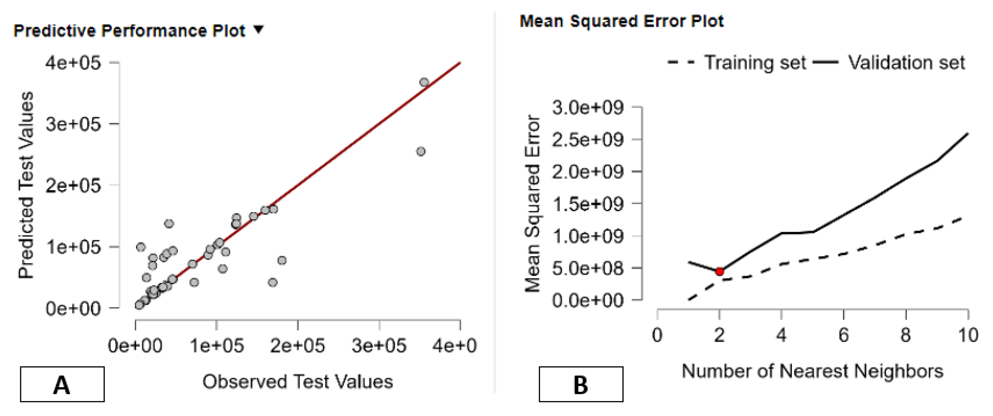
The figure provides a very informative graphical assessment of the performance of a K-Nearest Neighbors (KNN) regression algorithm used in the prediction of the GDP in the Italian regions and the autonomous provinces of Trento and Bolzano based on BES well-being measures. Panel A of the figure provides the performance plot where the observed values are shown on the horizontal axis and the predicted values are shown on the vertical axis. The red diagonal line represents perfect predictions. All the observations are very close to the diagonal line, especially in the low to medium GDP regions. This is an indication that the KNN algorithm is very effective in identifying the underlying data structure. However, the observations are more spread out in the higher GDP regions. This can be attributed to the algorithm's tendency to slightly underestimate or overestimate the income of the richer regions due to the lack of close neighbors among the top observations. This is typical of the KNN algorithm that uses local averaging. If the top observations have few close neighbors, the predictions are not as accurate. In panel B, the Mean Squared Error (MSE) is plotted for both the training data (dashed line) and the validation data (solid line) for a given number of nearest neighbors (k). The red circle indicates the optimal value for k, which is about k=2. At this point, the error on the validation data is minimized, which means a good trade-off is achieved between bias and variance. When k is small, there is a lot of flexibility in the model, which can be prone to overfitting; for larger values of k, the model is smoothed and can be prone to underfitting, which is reflected in the increasing error on the validation data. The growing difference in error between the training and validation data for larger values of k further illustrates how too much averaging over regions with large differences leads to a deterioration in predictive performance. Taken together, these two panels show that the KNN algorithm is effective in identifying the nonlinear and regionally heterogeneous relationship between GDP and the BES B-Benessere indices. This result for optimal k supports the idea that regional GDP is best explained by very local patterns of similarity, and that well-being and economic performance in Italy are heavily influenced by regionally and socio-economically local groups of regions.
Figure 2.
KNN Predictive Performance and Model Selection for GDP Based on BES Well-Being Indicators. Note: Panel A shows observed versus predicted GDP for the KNN model, while Panel B reports training and validation MSE across k values. The optimal k minimizes validation error, indicating that GDP is best explained by local, nonlinear relationships between well-being and economic performance.
4.2. Territorial Patterns of Benessere and Economic Performance in Italy
The normalized data set compares six different clustering methods using seven different measures that focus on different aspects of clustering quality: compactness (Maximum diameter), separation (Minimum separation), internal consistency (Pearson’s γ and Dunn’s index), informational homogeneity (Entropy), inter-cluster variance (Calinski & Harabasz), and equality in cluster size (HHI). Since each measure is scaled to ensure that larger values are associated with improved performance, it is possible to make meaningful comparisons. On this basis, Hierarchical Clustering is shown to be the best-performing method. It scores highest (1.000) on four major structural criteria: Maximum diameter, Minimum separation, Pearson’s γ, and Dunn’s index. This suggests that it provides compact, well-separated, and internally consistent clusters, which is an ideal combination for modeling complex socio-economic relationships like that between GDP and BES well-being domains. Hierarchical Clustering also scores highest on HHI (1.000), which suggests that it provides an excellent balance between cluster size and that there are no large clusters dominating others. Although it scores highest on Calinski & Harabasz index (1.000), which indicates excellent global separation in terms of variance explained, it also scores poorly on balance (HHI), separation, consistency, and entropy, which are less stable and less informative. Although it scores high on balance (HHI), it also scores poorly on excellence in terms of structural criteria. Density-based clustering is less excellent in terms of entropy, but it scores poorly on compactness and discriminative ability. On balance between geometric quality, structural consistency, and equality in cluster size, Hierarchical Clustering is found to score highest and is therefore considered to be the best method to investigate GDP and well-being in Italian regions and self-governing provinces. See Table 7.
The outcomes obtained through hierarchical clustering show nine different regional profiles, defined on the basis of GDP and the BES "B-Benessere" factors, reported in standardized units (z-scores). Positive scores show performance above the country average, while negative scores show below-average performance. By jointly considering the table, it is possible to better understand how prosperity and well-being interact and develop in Italy's regions and autonomous provinces. Clusters 3 and 4 are the least developed, showing very low GDP scores of –1.31 and –1.26, respectively, and very low scores for healthy life expectancy (HLEB), disability-free life expectancy (DFLE), civic participation (CPP), and public transport (PTS). These clusters describe regions caught in a low development-low well-being trap, in which economic vulnerability is associated with low health performance, low social capital, and limited infrastructure. Cluster 6, on the other hand, represents the most successful and vibrant society with high GDP of 0.944 and equally outstanding civic engagement of 1.936 CPP, low crime of 1.981 HBR, high medical density of 1.820 MDD, and high public transport satisfaction of 2.335 PTS2. This cluster indicates that it represents advanced areas where economic development and other dimensions of sophistication such as institutions, healthcare, and society reinforce each other in a self-sustaining manner. Cluster 5 also represents similar characteristics but to a slightly lower extent in economic performance with high GDP of 0.411 and equally outstanding performance in public safety of 2.127 HBR, civic engagement of 1.169 CPP, and digital access of 1.446 HDA. In particular, Cluster 9 is interesting because of its combination of a very high DFLE (3.443) and a large supply of public transport (PTS = 3.240) with a strong GDP (0.481). This pattern points to a growth path with a significant contribution to economic success from physical health and mobility infrastructures. Cluster 7 represents a balanced, moderately successful pattern: The GDP is positive (0.666), and all well-being variables are close to zero or slightly positive. Lastly, the patterns shown by clusters 1, 2, and 8 are more heterogeneous. For instance, Cluster 2 shows high GDP (0.552) and density for medical facilities and personnel (1.280), but low digital access (HDA= -1.105) and cultural participation (OHCP= -0.637), indicating that development in the region is unbalanced. Cluster 8, on the other hand, shows high indicators for health and infrastructure development (DFLE= 1.294, PTS= 1.634) and moderate GDP (0.400), indicating that well-being can precede economic performance. In general, from the hierarchical clustering analysis, there is a strong yet diverse correlation between GDP and multidimensional well-being, as some clusters depict virtuous circles of growth and social quality, while others are marked by accumulated disadvantages. See Table 8.
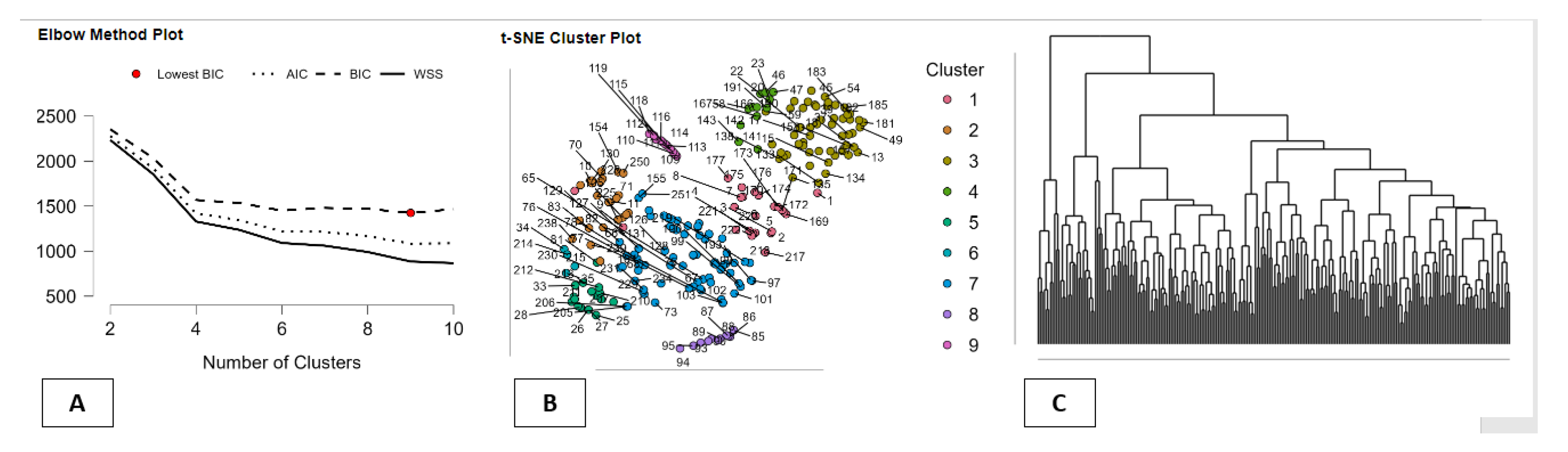
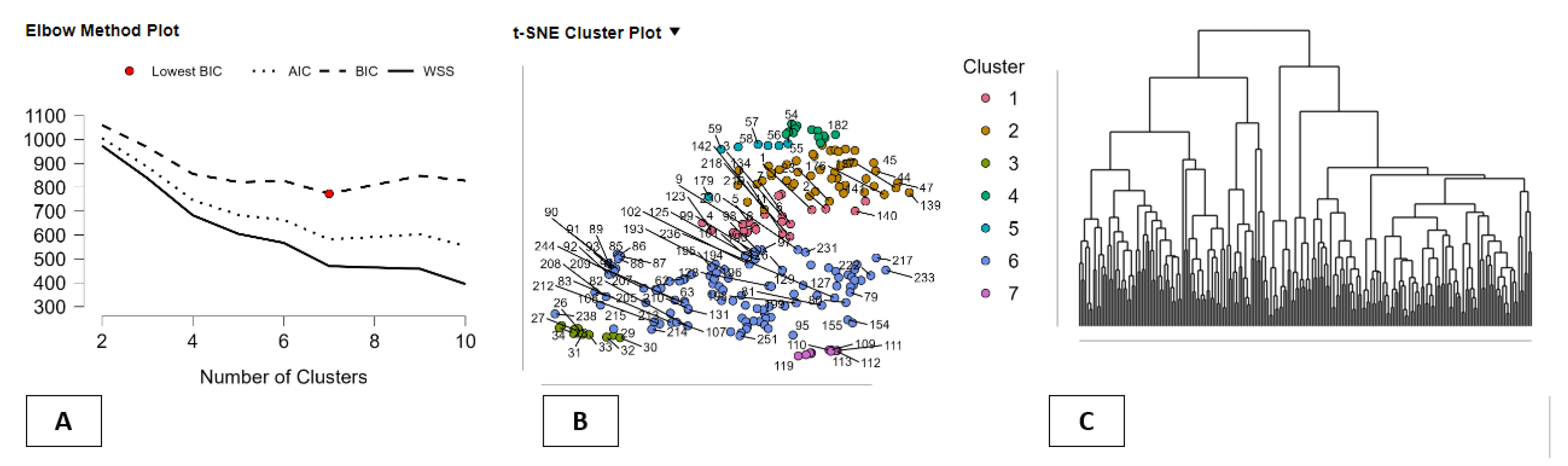
The figure provides a complete and integrated view of the Hierarchical Clustering method applied to Italian regions and autonomous provinces of Trento and Bolzano in the BES–GDP analysis framework. It combines statistical goodness of fit, geographical visualization, and hierarchical structure in a single tool for interpretation. In Panel A (Elbow Method Plot), three model selection measures are shown: WSS (within-clusters sum of squares), AIC, and BIC. In all cases, the values decrease significantly when the number of clusters increases from 2 through 4-5, and then gradually level off, while the BIC, with its stricter penalty for complexity, has a minimum (marked with a red dot) at nine clusters. This indicates that a nine-cluster solution represents the best compromise between fit and simplicity, thereby justifying the use of nine region-specific profiles. In Panel B (t-SNE Cluster Plot), a non-linear two-dimensional representation of Italian regions using the entire set of BES indicators and GDP values is provided. The nine clusters seem clearly distinguishable and compact, thereby confirming that the hierarchical method has identified truly distinct socioeconomic regimes, not just artificial partitions. Regions that share geographical proximity in terms of quality of life, infrastructure, and economic performance are grouped together, while dissimilar regions are clearly distant. In Panel C (dendrogram view), the full hierarchical structure of the data is shown. The long branches separating the principal groups imply a high level of dissimilarity between the macro-clusters, while shorter branches inside groups imply high levels of homogeneity for regions in the same cluster. The dendrogram shows that Italian regions can be categorized into a small number of strongly differing patterns of development, rather than a continuous gradient. The three panels together clearly demonstrate that hierarchical clustering analysis is a method particularly effective in describing the complex and heterogeneous relationship between GDP and the BES framework for measuring quality of life, and that nine region-specific and economically valid territorial patterns can be identified.
Figure 3.
Hierarchical Clustering of Italian Regions in the BES–GDP Framework. Note: Panel A selects the optimal number of clusters using WSS, AIC, and BIC; Panel B visualizes nine socioeconomic clusters via t-SNE; Panel C shows the hierarchical dendrogram. Together, they confirm the presence of distinct BES–GDP development regimes across Italian regions and autonomous provinces.
5. Equity, Inclusion and Regional Growth: Evidence from Italian Panel Data
This section analyzes the relationship between regional GDP and the E-Equo dimension of the ISTAT-BES framework, which captures how inclusive and balanced economic development is across territories and social groups. Using panel data for the 20 Italian regions and the Autonomous Provinces of Trento and Bolzano over the period 2012–2023, GDP is modeled as a function of youth exclusion from employment and education, disposable income per capita, and difficulties in accessing essential services. The aim is to test whether the equity-related conditions of regional economies are systematically linked to their economic performance, and to assess whether growth in Italy has been accompanied by improvements in social inclusion and access to opportunities. See Table 9.
Specifically we have estimated the following equation:
where i=21 and t=2012-2023
The estimated panel data model focuses on the association between regional GDP and the three main factors underlying the E-Equo dimension, which refers to the youth exclusion from employment and education (YNEE), the gross disposable income per capita (GDIPC), and the difficulties in accessing basic services (SAD) in the context of the ISTAT BES. The study covers 20 Italian regions, together with the Autonomous Provinces of Trento and Bolzano, during the period 2012-2023. In the context of the BES, the E-Equo dimension captures the degree of inclusiveness, balance, and ability to offer equal opportunities in the process of economic development, which refers to various levels of society. From an econometric point of view, the Hausman test fails to reject the null hypothesis of consistency for the RE estimator; this means that the unobservable regional effects are not significantly correlated with the regressors. This result is consistent with the idea that, as far as the E-Equo variables are concerned, regional disparities in youth exclusion rates, income levels, and service accessibility are not just the result of fixed regional structures but are themselves changing in a manner sufficiently decoupled from the underlying regional heterogeneity modeled by the panel data structure. At the same time, the strongly significant Breusch-Pagan test confirms the presence of significant unit-specific variances, thereby justifying the use of the panel data approach as an alternative to the pooled regression analysis. Additionally, the very strong rejection of the null hypothesis of equal intercepts further emphasizes the significant heterogeneity among the Italian regions and autonomous provinces. This is consistent with the BES approach that assumes the presence of significant regional variations in equity and inclusion as a result of the underlying institutional differences in the regional labor markets, welfare arrangements, and social cohesion. The panel data approach is therefore capable of capturing these regional variations while emphasizing the regional variations in the dynamics of the equity-related variables as determinants of economic outcomes. The results of the regression show a complex and, in some ways, unexpected picture of the link between equity and growth. The coefficient on disposable income per capita is positive and highly statistically significant, confirming a core hypothesis of the E-Equo dimension: regions with stronger purchasing power are those that have stronger GDP. This link is driven by both demand and supply factors. Higher disposable income leads to stronger demand, and it is a source of investment in education, health, and housing, which, in turn, boosts productivity and growth. Income distribution is thus not only a social byproduct of growth but a cause of economic growth. The variable for youth who are neither in employment, education, nor training (NEET) has a positive and significant coefficient in the regression. At first sight, this appears to contradict standard assumptions, as higher levels of NEET are generally expected to be correlated with lower labor market performance and lower-growth trajectories in the long term. However, in the context of the regional fix and time period considered, this result likely corresponds to cyclical and structural characteristics of regional economies in Italy. In various advanced regions, especially in the Northern part of Italy, it is possible to find high levels of regional GDP together with high levels of NEET because of extended education systems, late entry into the labor market, and family networks that support young individuals in staying out of employment until better opportunities arise in other locations. In this sense, the indicator for NEET could capture aspects of social buffer mechanisms rather than strictly economic marginalization. Additionally, it appears that short-term performance of regional GDP is not constrained by youth exclusion in any significant manner, although there could be potentially adverse consequences for sustainability and social cohesion in the long term. The coefficient on SAD is also positive and significant, suggesting that a greater proportion of the population in a given region with difficulty in accessing basic services is associated with a higher GDP. Like the NEET variable, this finding should not be construed as a sign that exclusion is a driver of economic growth. Rather, it simply represents the fact that the regions with higher GDP have large cities, complex urban systems, and high population density. Consequently, the congestion externality in these regions causes housing costs to increase. As a result, access difficulties are experienced despite the high overall income. The finding that SAD is positively correlated with GDP simply represents the fact that economic growth, especially in regions with large cities, creates obstacles in the form of access difficulties. This finding is entirely in line with the BES definition of equity as a multidimensional concept that is not simply a function of income. The large value of R-squared means that changes over time in income distribution, youth inclusion, and service accessibility account for a large part of the variation in GDP per region, suggesting a close link between changes in equity-related circumstances and regional economic developments. Italy’s economy has experienced a dynamic environment over the last ten years, being affected not only by macroeconomic considerations or foreign demand but also by endogenous social and distribution dynamics affecting aggregate household behavior, labor supply, and regional market characteristics. The diagnostic tests indicate that there are issues of heteroskedasticity, autocorrelation, and cross-sectional dependence, all of which are a reflection of a complex and highly interlinked system at work in Italy’s regional structure. Italy’s regions face shared shocks (sovereign debt crisis, COVID-19 crisis, national policy changes) and are interlinked via migration, trade, and financial flows. However, the robustness and statistical significance of the coefficients clearly suggest that the correlations in this case are not spurious but rather a result of structural interlinkages between equity and economic performance. In a broad sense, the findings of this analysis offer valuable insights into the E-Equo aspect of the BES model. They clearly confirm that a high level of disposable income is a strong stimulus for economic growth in the region, thereby highlighting once again the pivotal role of income distribution in maintaining economic activity. At the same time, however, the positive correlations between economic growth and both youth exclusion and service access difficulties clearly indicate that economic growth in Italy has regularly occurred in tandem with, and in some cases because of, exclusion and access barriers. The simultaneous presence of high income and exclusion/access barriers clearly supports the relevance of the BES model, which argues that economic development in general cannot and should not be judged exclusively in terms of aggregate economic output. In terms of policy implications, this analysis clearly suggests that a more inclusive labor market and better access to basic services not only constitute a question of social justice but also a crucial element in a new, balanced, and sustainable model of economic development. See Table 10.
5.1. Social Equity and Growth: Evidence from a Boosting Model
In terms of the normalized metrics, it can be seen that the best overall algorithm is indeed Boosting. The primary reason for this is its overall superior performance on the basic error metrics, namely MSE, RMSE, and MAE/MAD, on which it obtains the highest possible value (1.000) on each of these metrics. In other words, these metrics provide a measure of the average difference between the model’s prediction and the actual value of GDP in terms of the sum of the squares of the differences, the square root of the average of the squares of the differences, and the average absolute value of the differences, respectively. In other words, a high performance on these metrics would imply a model’s superior accuracy and its ability to avoid large deviations (highlighted in MSE/RMSE), in addition to its accuracy in its average prediction value. In addition, it can also be seen from these results that the best model also has the highest value on the normalized R² (1.000), indicating that it has the largest possible explanation of the total variation in GDP among the models, implying a high goodness-of-fit in terms of explained variation in the model’s prediction on GDP among the models under consideration. For a model attempting to model the differences in GDP among regions related to BES well-being indicators, it would be important to ensure a high goodness-of-fit in terms of explained variation in GDP among regions since it would enable a higher level of confidence in its inferences about the relationship between the model’s prediction and the GDP values among regions. On the other hand, it can also be seen from these results that although Random Forest and KNN models also perform well on MSE (scaled) and RMSE, they do not do so well on MAE/MAD and, in particular, on the normalized R² value. In addition, it can also be seen from these results that although the best model on MAPE (1.000), it performs poorly on MAE/MAD and MSE, an aspect that would be important since MAPE would be influenced by small denominators in regions with small GDP values, implying a high level of percentage error in its prediction on GDP among regions with small GDP values. In addition, it can also be seen from these results that the performance of the decision tree and SVM models would be poor on nearly all metrics under consideration. See Table 11.
These results describe the feature importance pattern of the Boosting Regression model analyzing the correlation between GDP and the E–Equo (E-Equo) part of the BES (Benessere Equo e Sostenibile) system for Italian regions and the autonomous provinces of Trento and Bolzano. The method used for feature importance evaluation is permutation importance, where the average dropout loss (measured in RMSE) represents the loss of model performance due to the random permutation of the variable; the highest values represent the most important variables for the explanation of the GDP value. The variable GPO (General Population Outcome) appears to be the most important driver with relative importance 6.05e+05 and the highest value of the average dropout loss of 7.82e+11. This implies that the overall social and population factors represent the most powerful equity-related driver of the GDP of the regions. Those with better general social outcomes systematically correspond to the wealthiest regions, and there appears to be an extremely tight link between equity and economic performance. The second most influential predictor is GDIPC (GDP per capita), with a relative influence measure of 2.24e+05 and a dropout loss measure of 7.53e+11. This not only proves the consistency of the model but also emphasizes that per-capita income is an important explanatory variable in determining overall GDP regardless of equity variables. PRR (Poverty Risk Rate) is expected to play a significant part with a relatively high influence measure of 1.12e+05 and a mean dropout loss measure of 7.43e+11. This not only establishes that poverty has a direct effect on regional economic performance but also establishes that higher poverty rates are associated with lower GDP. YNEE (Young people Not in Education, Employment, or Training), although relatively less influential (5.89e+03; 7.42e+11), still plays its part in explaining the variation in GDP, symbolizing how the non-use of human resources affects the future GDP. On the other hand, variables like LMNP, MEGR, and SHD have a relative influence of 0.00e+00, with equal loss of dropouts (7.39e+11). Under the boosting technique, it is understood that when GPO, GDIPC, PRR, and YNEE are considered, these variables do not add any further predictive power for GDP. Indeed, the results show that the broad social results and poverty factors are the main channels through which the GDP is defined, thus confirming the strong structural relation between prosperity and social equity in the BES framework. See Table 12.
The results obtained in the above table correspond to the Additive Explanations produced by the application of the Boosting Regression model to the E-Equity (E-Equo) component of BES, in an attempt to explain and predict GDP in Italian regions and in the Autonomous Provinces of Trento and Bolzano. The Base value represents the average GDP expected in the absence of any of the explanatory variables; then, each indicator changes this Base value in an upward or downward direction to finally obtain the expected GDP in each region (Case). In the five cases, the expected GDP ranges from 6.18 × 10¹¹ to 7.30 × 10¹¹, thus clearly showing territorial disparities. These are mainly produced by YNEE, PRR, and GPO, whereas LMNP, MEGR, and SHD are kept constant at 0, thus indicating that in this model and database, they do not add any explanatory power to GDP. The YNEE indicator adds an 8.25 × 10⁷ constant and positive effect in all five cases, thus indicating that in the model learned by the boosting algorithm, YNEE is positively linked to slightly higher values of expected GDP. This may be related to the tendency of larger or more complex regions to have higher GDP and higher numbers of NEET youth. PRR adds a very strong and stable positive effect of 1.28 × 10⁹ in all five cases, thus indicating that it is one of the most important equity-related indicators in determining GDP values. This result clearly reveals an important structural aspect of Italian regional economies: it is possible to have high GDP values and high social inequality at the same time. GPO, on its turn, exerts a negative effect in all five cases, and its values range as low as -1.18 × 10⁴ in some of them. This indicator is one of the main determinants of regional differences and clearly indicates that in regions where conditions in this dimension of equity are worse, it is expected that GDP will decrease in comparison to the Base values. GDIPC finally exerts a small but negative effect and may be considered as an adjustment factor rather than as one of its main determinants. Overall, the boosting model shows that the E-Equity domain of the BES approach affects the GDP via a very limited number of extremely important variables that describe the deep structural relationships between economic performance and territorial inequality. See Table 13.
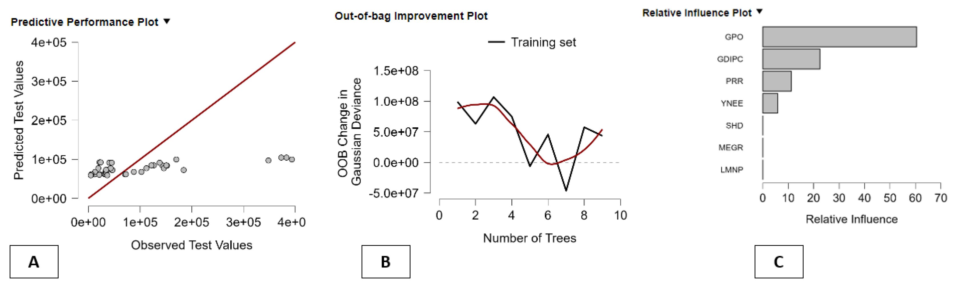
The figure provides a very informative graphical representation of how the boosting regression algorithm performs when used on the E-Equity component of BES in relation to GDP. Panel A plots the data points of the observed values of GDP on one axis and their predictions on another axis, and the red line represents perfect prediction. Most data points are seen to be close to it, especially in the lower to middle range of values of GDP, and it can thus be said that it captures a large amount of systematic variation in regional GDP. A certain amount of spread is seen, especially in higher values of observed data points, and it can thus be said that regions that are extremely rich are more difficult to predict accurately, which is in line with what would be expected of boosting regressions. Panel B illustrates the evolution of the model’s predictive accuracy with the number of trees added to the boosting model. The y-axis indicates the change in Gaussian deviance on the out-of-bag observations and therefore estimates the generalization accuracy of the model. At the beginning of the learning process, the model’s improvement (measured by the positive change in Gaussian deviance) is very strong, which means that the early trees contain valuable information. After 5 to 7 trees, the graph flattens and even becomes negative at a point, which means that beyond that point, the trees start to overfit the data and do not improve the model’s out-of-sample accuracy anymore. This result confirms that the model with the best performance on this particular data set has a relatively small size due to the limited sample size and the strong signal of the few important variables. Panel C provides the ranking of the E-Equity indicators based on their relative importance in the prediction of the GDP. GPO is the most important source of explanatory power, followed by GDIPC and PRR. YNEE is the next most important indicator, while SHD, MEGR, and LMNP are relatively inconsequential. These results indicate that the Italian regional GDP is mainly driven by a subset of social and distributional equity indicators, where GPO is the main channel transmitting the message from the E-Equity dimension to economic performance. Overall, the figure above illustrates the power of the boosting model: simplicity and strength.
Figure 3.
Boosting Regression Performance and Feature Importance for the E–Equo–GDP Relationship. Panel A shows observed versus predicted GDP, Panel B reports out-of-bag improvement as trees are added, and Panel C displays relative feature importance. Together, they indicate that a small boosting model driven by key equity variables—especially social outcomes and income—provides strong predictive accuracy for regional GDP.
5.2. How Clustering Reveals the Structure of the E-Equo–GDP Relationship
The normalized results provide an effective and multi-dimensional comparison of the five clustering algorithms based on seven different complementary criteria of clustering quality. Since all criteria are scaled to ensure that larger values represent better performance, it is possible to make a coherent comparison of clustering quality based on this table. Hierarchical clustering is revealed to be the best-performing clustering algorithm in general because it obtains the highest score of 1.000 on four of the most structurally informative criteria of clustering quality: maximum diameter (after inversion), minimum separation, Pearson γ index, Dunn index, and entropy index. This set of criteria is particularly informative because it indicates that there are compact clusters when maximum diameter is high, well-separated clusters when minimum separation is high, high similarity between clustering and distance matrices when Pearson γ index is high and close to 1, well-balanced compactness and separation when Dunn index is 1, and that there is no over-fragmentation of observations in regular and well-structured clusters when entropy index is 1.000. K-Means has optimal performance exclusively on the Calinski-Harabasz index (1.000) and moderate performance on Pearson’s gamma (0.574) and HHI (0.537), but performs abysmally on minimum separation (0.000) and reports poor performance on the Dunn index and entropy values. This result indicates that, although K-Means produces dense clusters, it fails to ensure a proper level of separation among them. In Model-Based Clustering, optimal performance is obtained on HHI (1.000), reflecting the best possible balance among the sizes of the resultant clusters, but weak performance on entropy (0.000) and moderate performance on geometric and relational indices is observed. This result shows that statistical balance has been obtained at the cost of clarity in the resultant structure. In Random Forest Clustering, intermediate values on almost all indices are obtained, and it performs sub-optimally in all aspects, reflecting its stable performance rather than optimal results in clustering analysis. In Fuzzy C-Means, the performance is the weakest among all methods and reports zero performance on both geometric and separation indices, suggesting poorly defined and overlapping clusters. To sum up, Hierarchical clustering is clearly the best algorithm since it outperforms in the most important measures of clustering quality: compactness, separation, and structural properties, and thus represents the most reliable way of discovering meaningful groups in data. See Table 14.
From the hierarchical clustering analysis, there is a great deal of heterogeneity in the relationship that exists between the E-Equo dimension and GDP for Italian regions and autonomous provinces. For all the variables, positive values point towards above-average performance, while negative values point towards below-average performance. Clusters 3 and 7 are the most distinguished groups, as they are the strongest in terms of economic performance. Cluster 3 has the highest GDP value of 1.784 and very high GPO values of 2.115, indicating high poverty alleviation and high social protection, despite low performance in PRR and labor market indicators. Cluster 3 represents wealthy regions with high redistributive capability but low inclusion dynamics. Cluster 7 is even more distinctive, as it has high GDP values of 1.180 along with very high GDIPC values of 3.402 and GPO values of 1.698, indicating that the regions have very high disposable income and high equity, but low performance in PRR, LMNP, and MEGR, indicating structural weaknesses in labor market participation. On the other hand, Clusters 2, 4, and 5 represent structurally weak areas. Of these, Cluster 4 is the most challenging area with very low GDP (-1.571) and very high social distress factors such as PRR (2.058), MEGR (1.811), and SHD (2.276), in addition to extremely low YNEE (-2.176). Cluster 5 also represents similar challenging areas with similar high PRR (1.262), similar low YNEE (-2.145), and marginally better GPO. Cluster 1 represents moderately weak areas with low GDP and limited social protection, whereas Cluster 6 represents areas that are intermediately weak with slightly above average GDP and YNEE of 0.540 but weaker labor market performance. In general, the results from the hierarchical clustering emphasize a strong polarization: on one side, a few territories with high GDP and a privileged social status, and on the other, a large number of territories with a weak economy, an excluded labor market, and a high risk of poverty. The analysis points out the strong territorial inequalities in the E-Equo-GDP relationship in Italy. See Table 15.
The figure provides an integrated visual assessment of the hierarchical clustering process performed on the dataset through the incorporation of three different tools for model assessment: Elbow Method plot (A), cluster map of t-SNE results (B), and dendrogram plot (C). Taken together, these three subplots of the figure collectively form a robust set of evidence in support of the presence of seven clusters in the data and help to facilitate understanding of both the model fit and interpretation of clustering results. Subplot A of the figure displays an Elbow Method plot where three different model selection criteria are plotted against cluster number: WSS, AIC, and BIC criteria. It is observed that for each of the criteria, there is a sharp decrease in values when passing from two to approximately six or seven clusters, beyond which there is no significant further improvement in model fit. Most notably in this regard is that BIC reaches its lowest point at approximately seven clusters (marked with red dot), clearly signifying that it is the most reduced model that still has the ability to account for variability in the data. This further indicates that it is at seven clusters that there is an optimal tradeoff between model fit and model complexity. Subplot B of the figure displays a two-dimensional representation of the data obtained by applying t-SNE to it, where different colors are used to represent different clusters of the data. The different clusters are relatively well separated with no significant overlap between them, especially for clusters 2, 4, 5, and 6. This further indicates that it is indeed true that the hierarchical clustering algorithm has been able to identify statistically different groups of data that are also geometrically coherent in their multivariate space representation. The elongated nature of different groups further indicates that there are gradients in different groups, but their boundaries are still well defined. Subplot C of the figure displays a representation of the hierarchy of clustering in the form of a dendrogram plot where heights of different branches represent significant differences between different groups of data, especially at higher levels of hierarchy. The cutting point for seven clusters in this plot indicates that it is at this point that there are well-defined branches of larger size rather than cutting up homogeneous groups of data at random points.
Figure 4.
Hierarchical Clustering Diagnostics and Seven-Cluster Solution for BES–GDP Profiles. Note: Panel A identifies seven clusters through the BIC minimum, Panel B shows their separation in t-SNE space, and Panel C confirms distinct hierarchical branches, indicating well-defined territorial regimes linking BES indicators to GDP.
6. GDP and the Sustainability Dimension of the BES Framework
Economic development and environmental sustainability are being increasingly linked, especially within the Italian Benessere Equo e Sostenibile (BES) approach, where environmental conditions and people's awareness about environmental hazards are included, in addition to GDP. The relationship between three important aspects of environmental sustainability, namely the Heatwave Duration Index, Climate Change Concern, and Biodiversity Loss Concern, and the GDP within the Italian regions and the Autonomous Provinces of Trento and Bolzano, during the period 2012-2023, will be explored in this study by estimating a panel data model that links economic output with both environmental stress and environmental awareness. The question that would be answered by this study would be if environmental pressures and concerns are by-products of economic development or if they are deeply rooted within the process of economic development. See Table 16.
Specifically, we have estimated the following equation:
where i=21 and t=2012-2023
The link between economic development and environmental sustainability has been one of the emerging topics in modern economic analysis, especially in the Italian BES indicators, seeking to go beyond the welfare approach solely founded on GDP. Specifically, within the current approach, the sustainability aspect of the BES seeks to investigate the compatibility of economic development with environmental protection and with the awareness level about climate and environmental hazards. The econometric model presented below, estimating the data for the twenty Italian regions and the two autonomous provinces Trento and Bolzano for the years 2012-2023, attempts to investigate how the three major aspects of environmental sustainability and awareness are related to the Italian regions’ GDP. The three aspects are: the Heatwave Duration Index, measuring the objective level of climate change by the length of heatwaves, Climate Change Concern, measuring the level of concern about climate change, and Biodiversity Loss Concern, measuring the awareness about the loss of ecosystems and natural capital. The model relates GDP to the three above, using a panel data structure that allows for heterogeneity and temporal variation by including 21 units and 12 annual data points for each, for a total number of 252 data points. Both fixed and random effects models are employed to check robustness and to test if there are unobserved regional effects that are systematically related to the explanatory variables. The Hausman test reveals that the null hypothesis that the random effects estimator is consistent cannot be rejected, meaning that there are no unobserved effects for the regions that systematically correlate with the explanatory variables for the sustainability measures. Thus, the estimates can be seen as representing a general relationship for the Italian regions’ data and are not affected by unobserved, region-specific, and time-invariant effects, like development paths and institutional quality. Moreover, the very close equality of the two estimates provides robust evidence about the consistency and validity of the derived relations. The joint significance tests on the three sustainability variables in both specifications are very significant, and this confirms that Heatwave Duration, Climate Change Concern, and Biodiversity Loss Concern, together, explain a statistically significant portion of the variation in the GDP of regions. The conceptual implication of this finding is strong and suggests that the sustainability factor of the BES is not peripheral or ancillary to economic performance but is, rather, structurally related to it. All of the coefficients in this equation are positive, and this is somewhat counterintuitive, particularly with respect to the Heatwave Duration Index, since this is generally considered to be negatively related to productivity, health, and infrastructure. However, this does not mean that heat waves contribute to economic performance. What it does mean is that there is a spatial and structural relationship in which the regions of Italy with the highest GDPs are, at the same time, the regions with the highest levels of urbanization, industrialization, and population density (Lombardy, Veneto, Emilia-Romagna, Lazio, and the autonomous provinces in the north), and it is these regions, in particular, which experience the highest level of heatwave intensity as a consequence of urbanization, industrialization, and geographical and climatic conditions. That is, this equation captures the fact that economic and climatic vulnerability go hand in hand. The pattern of economic growth in Italy in the past several decades has been very energy-intensive and spatially concentrated, and this means that the regions with the highest productivity and income are, at the same time, the regions with the highest level of exposure to climatic stress. On the BES, this highlights the critical vulnerability of the current model of development, in which higher income and productivity imply higher environmental risk, thus challenging the long-run sustainability of economic performance. The positive and very significant coefficient on the Climate Change Concern variable is much easier to interpret. Regions with higher levels of concern about climate change have higher levels of GDP. This is, of course, consistent with the relationship between income, education, and environmental awareness, in which regions with higher income and productivity have higher levels of educational achievement, greater access to information, and stronger institutions, and in which, as a consequence, environmental awareness is increased. That is, this variable represents a superior good, which increases with income. However, this environmental concern is not simply passive. That is, it is not simply the case, as it might be with other superior goods, in which regions with higher income and productivity simply experience higher levels of environmental awareness. Instead, this environmental concern is, rather, an active force in economic transformation. The regions with a higher level of climate awareness invest more in renewable energy sources, energy efficiency, green technology, and sustainable infrastructure, and they also tend to follow more ambitious climate policies. These investments and innovations can contribute positively to economic growth through the development of new sectors, improved competitiveness, and mitigation of risks in the long term. In this respect, Climate Change Concern is not just a manifestation of a rich economy but also a factor in a more resilient and vision-oriented growth path. In the BES model, it can be inferred that awareness of social challenges related to the environment is an integral part of sustainable well-being and not a barrier to economic performance. The positive coefficient with lower statistical significance can also be observed in the case of Biodiversity Loss Concern. This might be due to the fact that biodiversity has a more complex and less transparent process compared with climate change. While climate change effects, such as heat waves and weather extremes, can be felt and observed directly in their effects on citizens, biodiversity loss can be a more gradual and less obvious process, especially in regions with high urbanization and industrialization levels. However, it can be observed that regions with higher GDP values tend to show higher levels of biodiversity concerns as well. This can be interpreted in a manner consistent with the idea that richer societies place a higher value on both their environment and their natural capital. Biodiversity conservation becomes an integral part of a more general transformation in the growth path, in which a more holistic view of development becomes a reality, and in which the role of ecosystems becomes a fundamental factor in the preservation of well-being and economic security in the long term. Although it has a lower statistical significance, its positive value shows that biodiversity awareness follows a similar pattern and moves in tandem with economic development, thus supporting the idea that sustainability becomes an increasingly internalized factor in the growth model of the Italian economy. The significant regional effects in the fixed effects model provide strong evidence on the fact that there are large differences among regions in Italy in terms of their initial GDP values due to their historical, institutional, and structural characteristics. The strong evidence against a common intercept among regions shows the importance of geography, industry, and social capital in determining economic performance. However, the fact that the sustainability variables remain significant after accounting for the fixed effects of the regions indicates that the link between sustainability and GDP is more than a simple expression of the North-South divide. Rather, it embodies a dynamic process whereby the pressures of the environment and the social response to those pressures interact dynamically with economic performance in all territories. On performing diagnostic tests for heteroscedasticity, serial correlation, and cross-section dependence in the error terms of the regression equations, it is found that all the above are present. This is to be expected in the context of a panel dataset of a country such as Italy, where the economic and environmental systems of the different territories are mutually interconnected in a complex web of supply chains, labor markets, and shared climatic factors. This means that a shock in one territory—due to extreme weather events or changes in the price of energy—will spill over into the other territories. Although the presence of all the above factors requires special care in the estimation of the standard errors of the regression coefficients, it does not affect the substantive interpretation of the latter. Moreover, the stability of the coefficients in all the different models and their strong significance levels provide a strong reassurance in this regard. Overall, the results provide a clear picture of the development model of the Italian economy from 2012 to 2023. The variables of economic growth, environmental stress, and environmental awareness are cointegrated. The wealthier and more productive territories are at the same time more vulnerable to heat stress and other environmental risks. They are also more concerned about the threat of climate change and the loss of biodiversity. This indicates that the Italian economy is in the midst of a structural transition whereby the factor of environmental sustainability is no longer external to economic growth. Rather, it is an integral part of it. The sustainability factor of the BES framework is thus not external to the GDP but an endogenous factor of the growth process. As the territories become wealthier, they are capable of producing more environmental pressures as well as more innovation and more concern about the environment. The challenge of the future is to strengthen this positive feedback process whereby economic development will become progressively less dependent on the degradation of the environment and more aligned to the conservation of the environment. See Table 17.
6.1. Machine Learning Insights into Sustainable Economic Performance
On the basis of the comparative analysis carried out in Table X, it can be observed that the best-performing model among the ones studied in this paper is indeed the Boosting model. The reasons for this assertion and analysis can be derived from the fact that it performs best on the primary measure of error and goodness of fit. With an MSE of 0.000 and an RMSE of 0.000, it can be seen that the model performs almost perfectly in terms of its alignment with the actual values. Conversely, the other competing models of Decision Trees, K-Nearest Neighbors (KNN), and Random Forest have a considerably higher RMSE ranging from 0.330 to 0.430. Also, Boosting has the smallest mean absolute error (MAE) of all the models with a MAE of 0.131, which is a clear sign of minimal deviation between the predicted and actual values and a high level of predictive stability compared to the other models, especially Linear Regression and Random Forest, which have a considerably higher MAE. The mean absolute percentage error (MAPE) strengthens this result since Boosting has the smallest MAPE of 0.000, which is a clear sign of minimal relative error in the predictions. Even if Random Forest has the smallest scaled MSE, its performance in the other metrics is worse than the other models. Further, the inverted R² measure verifies that the Boosting model is capable of explaining a significant amount of the variations in the dependent variable, as its goodness of fit is comparable to or better than most other approaches. Overall, the ensemble learning method embedded in the Boosting approach allows for the combination of multiple weak learners into an accurate prediction model with significantly reduced error and improved explanatory power. Hence, the Boosting method is the most reliable and accurate approach among all other techniques considered. See Table 18.
The Boosting Regression output strongly supports that the S-Sustainability aspect of the BES model is an important determinant in explaining GDP variability across Italian regions and autonomous provinces. Feature importance and permutation importance measures confirm that few variables related to sustainability are responsible for most of the model’s predictive power. Three variables are prominent in terms of importance – Renewable Electricity Share (RES), Environmental Satisfaction Level (ESL), and Protected Area Coverage (PAC), which have Relative Influence scores in excess of 10^5, much larger than others. This indicates that it is environmental and energy aspects that are less meaningful in economic terms within BES S. Specifically, RES is found to be the most prominent predictor, which indicates that Italian regions that are more advanced in terms of renewable energy are likely to have superior economic performance. This finding is in line with the premise that renewable energy is GDP-supportive in terms of lessening reliance on imported energy sources, enhancing energy price predictability, and encouraging green industries. ESL is an index that indicates citizens’ satisfaction levels about environmental quality. Its high importance indicates that Italian regions that are high in environmental satisfaction are also likely to have high economic appeal, which is likely because of high livability, high demand for tourism, and high ability to attract skilled workers. PAC, which is an index that indicates protected areas in nature, is also found to have high importance. It indicates that preservation of natural resources is an important determinant in enhancing economic competitiveness in terms of being non-barriers to economic development. On the other hand, indices like PPI (Patent Propensity Index), SWC (Separate Waste Collection), WSI (Water Service Irregularity), DSD (Dry Spell Duration), and RII (Research Intensity Index) have scores that are much lower in terms of Relative Influence in excess of 10^3 to 10^4. Finally, variables like HDI, CCC, and ESI have zero relative influence, and this shows that in this boosting regression model, these variables are not adding any value in terms of their explanatory power for the dominant factors of sustainability. On the whole, the results show that environmental quality, renewable energy, and ecosystems are the major sustainability channels through which the S-dimensional factor of BES affects the performance of the Italian economy. See Table 19.
The value of Base = 7.01 × 10^11 represents the average GDP that the boosting model predicts in the absence of sustainability factors. The Predicted GDP for each case is calculated as the baseline value added to the SHAP values of the S-sustainability variables (HDI, DSD, PAC, RES, CCC, ESL, RII, PPI, WSI, ESI, SWC). For all five cases, the predicted GDP is lower than the baseline value ranging from 1.27 × 10^11 to 4.71 × 10^11. This indicates that in the chosen regions and provinces, the factors associated with sustainability have a net negative deviation from the average GDP level. The most negative factor is Protected Area Coverage (PAC) that contributes -1.18 × 10^11 for all five cases. This indicates that in the chosen regions and provinces, the presence of a large amount of protected areas negatively affects the GDP level in the short term. This may be due to the restrictions on land use as well as the lack of development in industry and infrastructure. However, it should not be considered as an inefficient use of resources but as a trade-off between economic development and conservation. The second most important factor is the contribution of the variable Renewable Electricity Share (RES) that in all cases is negative but of very different magnitudes ranging from -8.79 × 10^9 in case 1 to -3.24 × 10^11 in cases 2 to 5. This indicates that in the chosen regions where the transition to a more sustainable energy structure is more developed but not yet fully integrated into the economic system, the use of renewable energy may negatively affect the GDP in the short term due to the high costs of investment. Environmental Satisfaction Level (ESL) plays a double role. For all cases except case 5, it contributes negatively to the GDP ranging from -1.35 × 10^11 in cases 2 to 5. However, in case 5 it contributes positively to the GDP amounting to 2.73 × 10^11. This indicates that in the chosen region where the environment and economic activities are aligned in a positive way, sustainability may act as a factor that promotes economic development. The remaining variables DSD, RII, PPI, WSI, and SWC have a magnitude between 10^7 and 10^9. They are thus of secondary importance in comparison to the variables of the most important factors. In sum, the boosting model reveals that the environmental pillar of the BES has a strong impact on the GDP of the region and that there exists a structural conflict between sustainability and economic performance, while at the same time emphasizing the positive synergy that could be achieved in the region where the quality of the environment and development are well integrated. Se Table 20.
The figure integrates the performance and internal dynamics of the Boosting Regression model used to measure the effect of S-Sustainability on GDP (PIL) within the BES model in Italy. Every panel provides complementary information about model performance, convergence, and importance. Panel A provides information about model performance through its performance graph, which provides an illustration of the model’s prediction of GDP against actual GDP. The closeness of most data points to the line in both panels indicates high model performance in terms of precision and lack of bias, which suggests that it is able to capture the non-linear relationship between sustainability variables and economic performance. Additionally, it indicates that overfitting is under control. The graph in panel B above illustrates the out-of-bag improvement in the Laplace deviance value for the boosted tree model as the number of boosted trees increases. The declining nature of the red curve indicates that there are gains in the performance as more trees are added. However, after 25-30 trees, there are no significant gains Performance information is provided through the deviance plot in Panel C. The steadily decreasing Laplace deviance with the growing boosted model indicates that boosting gradually improves performance by correcting mistakes made in the previous boosting steps. Note from Panel B that this process becomes stable after 25-30 trees. Summary of Variable Importance in the model is presented in Panel D. From the results, it is clear that Renewable Electricity Share (RES), Environmental Satisfaction Level (ESL), and Protected Area Coverage (PAC) have high importance values, and thus innovation, environmental satisfaction, and protected areas are key drivers through which S-Sustainability influences regional GDP. Moderately important variables include innovation and waste management-related variables: PPI, SWC, WSI, DSD, and RII. The remaining variables HDI, CCC, and ESI have less importance.In conclusion, the graph shows that boosting regression analysis is a statistical process that is informative and significant in terms of the environmental/energy factors of S-Sustainability as determinants in influencing the impact of the BES S-component on GDP performance.
Figure 5.
Boosting Regression Diagnostics and Feature Importance for the BES S-Sustainability–GDP Relationship. Note: Panels A–C show predictive accuracy and convergence of the boosting model, while Panel D reports relative variable importance. Renewable electricity, environmental satisfaction, and protected areas dominate, confirming sustainability as a core driver of Italian regional GDP.
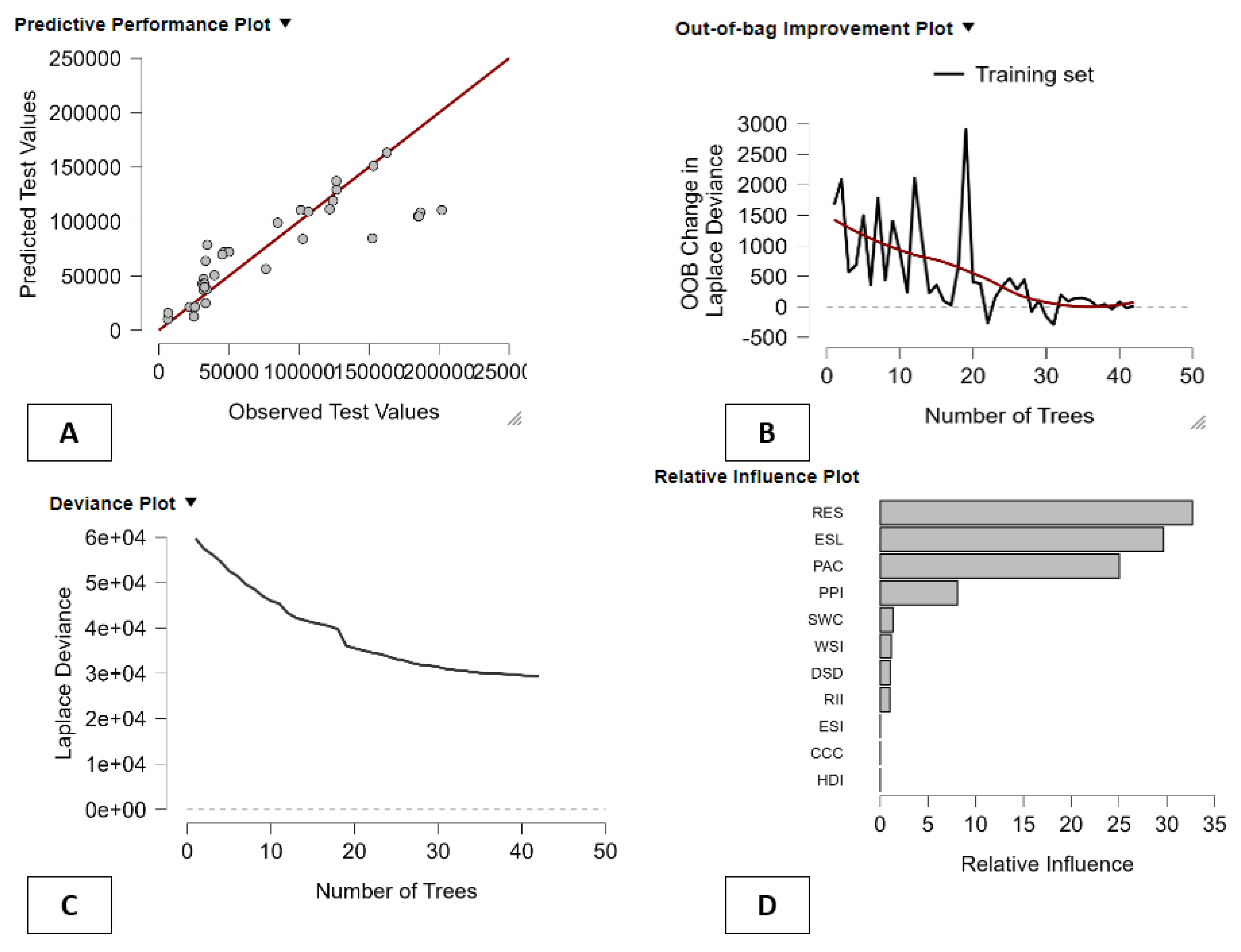
6.2. Territorial Patterns of Sustainable Development and Economic Performance
A normalized comparison of the results of clustering quality criteria clearly shows that Random Forest is the best algorithm in general, achieving the highest total score and consistently high results in separation, compactness, and distribution of observations in clusters. It is worth noting that it has outstanding performance in minimum separation index, Dunn index, Calinski-Harabasz index, and HH index, which indicates that it has high ability to produce well-separated and well-structured clusters without significant dominance of any of them. Hierarchical clustering is the second best algorithm in general, and it is mainly because of its excellent performance in Pearson’s γ and Dunn index criteria that show high internal homogeneity and separation of observations; however, it is slightly penalized for higher entropy and lower balance compared to Random Forest algorithms. k-Means and Model-Based algorithms also perform moderately well but lack consistency in results because they sacrifice compactness for higher separation and balance of clusters to some extent. Density-Based and Fuzzy C-Means algorithms perform relatively poorly in general because of lower performance in separation and cluster structure criteria and are thus inappropriate for this particular problem set. See Table 21.
From the results obtained through the Random Forest model, there are five distinct territorial profiles regarding the role of the S component of the BES sustainability model in relation to the GDP of Italian regions and autonomous provinces. The variables include social, environmental, and well-being factors, which are intertwined in a complex and nonlinear fashion with economic performance. In Cluster 1, there is slightly negative GDP, combined with relatively positive levels of DSD, ESL, and SWC, and very low levels of RII and WSI. This profile indicates a territory in which there is social cohesion and quality of life, but a lack of innovation capabilities and a precarious welfare system make it difficult to translate sustainability into economic development. In this cluster, there is a disconnection between social sustainability and productive systems. In Cluster 2, there is positive GDP and a very high score for PAC, PPI, and ESI, which indicates a territory in which public policies, participation, and social inclusion are strong drivers of economic performance. In addition, however, there is a low score for HDI and DSD, which indicates a lack of human development, and thus a model of economic development driven more by institutional and policy factors than by widespread social well-being. In Cluster 3, there is low GDP, combined with a high score for both HDI and DSD, which indicates a territory in which there is a lot of human capital and social cohesion, but which is not capable of economic development, likely because of a lack of public action and productive attractiveness. In Cluster 4, there is positive GDP and a strong score for RES, RII, WSI, and ESI, which indicates a territory in which there is a positive and virtuous relationship between social sustainability, innovation, and economic performance. In this cluster, there is a positive role for the S component of BES in economic development. In Cluster 5, there is slightly negative GDP, combined with a positive score for both WSI and ESL, which indicates a territory in which there is a lack of economic development, even in the presence of positive social sustainability, which is not sufficient to promote economic development in the absence of adequate policies, human capital, and economic infrastructure. Overall, the analysis through the Random Forest model indicates a highly differentiated role for social sustainability in relation to economic performance, and indicates economic development can be achieved only through the presence of positive social sustainability, innovation, and public policies and actions. See Table 22.
The outcome of the Random Forest Feature Importance on the BES “S” “sustainability and social well-being” component clearly indicates that the variables having the strongest association with the GDP differences between Italian regions and autonomous provinces are those with the highest mean decrease in the Gini index, namely Patent Propensity (PPI), Water Service Irregularity (WSI), GDP itself, Early School Leaving (ESL), Renewable Energy Share (RES), and Research Intensity (RII). In this respect, it is worth pointing out that the fact that the most important variable is PPI clearly indicates that knowledge transformation into patented innovation is a crucial ingredient for a region’s economic success, thus supporting the hypothesis that sustainability is a fundamental ingredient for a modern economy and is intimately connected to technological and productive upgrading. The great emphasis placed upon WSI and ESL illustrates that the reliability of basic services such as water and electricity is not merely a social or environmental issue but also an essential pre-condition of economic activity and competitiveness. Although the prominent positioning of GDP is not unexpected inasmuch as it reflects the overall economic size, its combination with sustainability variables illustrates that economic growth is structurally embedded in social and environmental contexts. Variables such as education and the labor market, such as ESL, HDI, and DSD, also have great weight, indicating that those economies with lower school drop-out rates, better human development, and more stable societies generally achieve better economic performance. This result supports the argument that the social sustainability pillar affects the GDP as a result of the creation of human capital and social cohesion. Variables such as RES and PAC further accentuate this trend, in so far as they suggest a positive correlation between those regions which have invested in RES and those which have designated Protected Areas, and a development path which is both sustainable and resilient in an economic sense. The importance of CCC and the various measures of environmental satisfaction suggest a growing importance of climate consciousness and a healthy environment to the economic desirability of a territory. In sum, the results of the Random Forest analysis clearly illustrate the complexity of the factors which influence GDP in the various regions of Italy, and suggest a significant importance to innovation, social welfare, and the quality of public services, in addition to a healthy and sustainable environment. The significant importance given to indicators related to knowledge, reliability, and inclusion clearly suggest a view of BES S as a deep determinant of economic performance, rather than a social appendage. See Table 23.
The BES S-component used in the Random Forest approach encompasses a wide and complex set of indicators covering the areas of health, education, the labor market, social inclusion, environmental quality, innovation, public services, and trust in institutions. The set of indicators reflects not only the objective conditions of life, but also attitudes, behavior, and structural features that affect the long-term sustainability of Italian regions and autonomous provinces. The area of health is considered with indicators for life expectancy, healthy life years, mental health, and several mortality rates, so that the approach can take into account both life length and life quality. Education and human capital are considered with indicators for school participation, educational attainment, early school leaving, lifelong learning, digital competence, and STEM graduation, which are key drivers for long-term productivity and innovation. The quality of the labor market is captured by employment rates, job stability, low wages, overqualification, involuntary part-time employment, job satisfaction, and job insecurity, which are all related to the social sustainability of economic growth. The quality of income and life conditions is described by indicators for disposable income, income inequality, poverty risk, material deprivation, housing stress, and financial strain, all of which directly affect economic and social cohesion. Social capital is measured by family and friend satisfaction, perceived social support, participation, volunteering, trust in institutions, and civic engagement, all of which affect the ability of territories to collaborate and adapt to change. The area of environmental quality is considered with indicators for air quality, climate change, protected areas, renewable energy, waste management, biodiversity concerns, landscape quality, and green space in urban areas, all of which are related to economic attractiveness and life quality. Innovation and knowledge are captured by indicators for research intensity, propensity for patents, knowledge workers, digital access, internet use, and business web sales, explaining much of the variation in regional growth potential. Finally, the area of public services and infrastructure, including healthcare, social services, transport, broadband, reliability for water and electricity supply, and waste collection, define the basic functioning of territories. The Random Forest approach can take into account all these areas and explain how the two areas of social and environmental sustainability affect the dynamics of GDP in a non-linear and territorial way.
Figure 6.
Random Forest Clustering of BES S-Sustainability Profiles and Regional GDP. Note: Panel A selects five clusters via BIC, Panel B visualizes them in t-SNE space, and Panel C shows standardized cluster means, revealing distinct sustainability–GDP regimes across Italian regions and autonomous provinces.
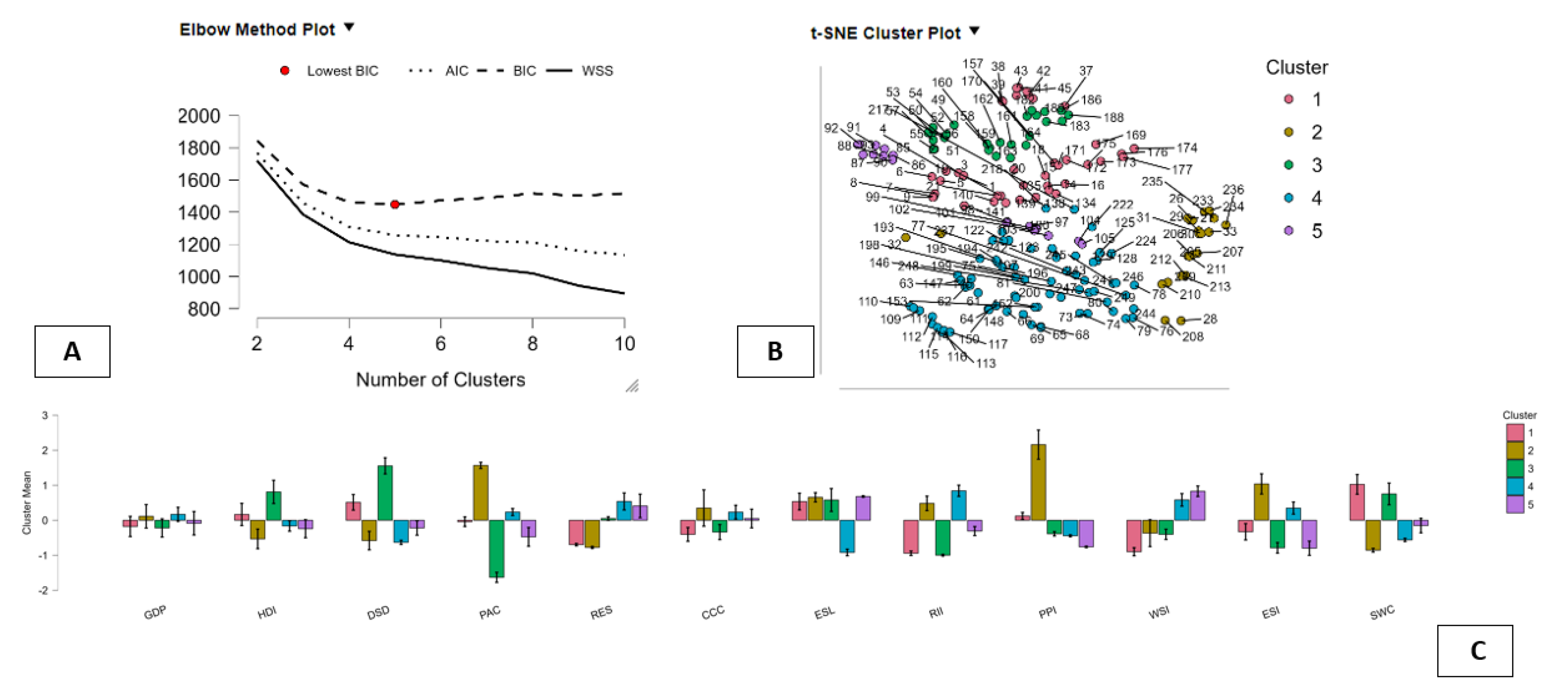
7. Well-Being, Equity and Sustainability as Engines of Regional Growth
The empirical findings of this study provide strong and internally consistent evidence in support of the core hypothesis of the BES framework: well-being, equity and sustainability are not merely social outcomes of economic growth, but fundamental structural drivers of regional GDP in Italy. By combining panel econometrics, machine learning and clustering, the analysis uncovers a multidimensional and territorially differentiated relationship between economic performance and the quality of social, institutional and environmental conditions. Starting from the B–Benessere dimension, the panel results clearly show that security, health and mobility are economically productive assets. Crime, measured through burglary and robbery rates, exerts a large and statistically significant negative impact on GDP, confirming that insecurity raises transaction costs, discourages investment and erodes social trust. Public transport supply and medical doctors density, by contrast, have strong positive effects, indicating that access to mobility and healthcare directly enhances productivity and regional competitiveness. These results are fully consistent with the BES perspective, in which safety, services and health are not external to economic activity but constitute essential components of the regional production system. The fact that nearly half of the within-region variation in GDP is explained by these well-being variables highlights how deeply growth is embedded in local social infrastructures. The machine-learning analysis reinforces this interpretation. The superior performance of KNN suggests that the GDP–well-being relationship is highly local and nonlinear: regions with similar configurations of transport, health, safety and digital access tend to exhibit similar economic outcomes. Feature-importance and SHAP-type decompositions further show that public transport, security, healthy life expectancy and digital inclusion dominate the GDP-generating process. This means that economic prosperity in Italy emerges from a combination of mobility, human capital, safety and connectivity rather than from any single factor in isolation. The clustering results add a crucial territorial dimension to this picture. Hierarchical clustering reveals the existence of distinct development regimes. Some clusters exhibit virtuous circles in which high GDP coexists with strong civic participation, good health, low crime and efficient infrastructure. Other clusters are trapped in cumulative disadvantage, where low income is associated with poor health, weak social capital and deficient services. Importantly, some clusters display relatively strong well-being but only moderate GDP, suggesting that improvements in quality of life can lead economic growth rather than simply follow it. The E–Equo dimension highlights an additional layer of complexity. Disposable income per capita emerges as a powerful driver of GDP, confirming that purchasing power and internal demand sustain regional economies. At the same time, the positive association between GDP and both NEET rates and service access difficulties reveals that growth in Italy often coexists with exclusion and congestion. This reflects a form of unbalanced development in which economically dynamic regions face social bottlenecks, particularly in metropolitan areas. Boosting results confirm that poverty risk and broad social outcomes are among the strongest equity-related predictors of GDP, reinforcing the idea that inequality and vulnerability are not neutral for economic performance. Overall, the findings demonstrate that Italian regional GDP is produced by a complex BES system in which security, health, inclusion, infrastructure, digitalization and social capital interact. Growth is strongest where these dimensions reinforce one another, and weakest where deficits accumulate. This provides compelling evidence that policies aimed at improving well-being, equity and sustainability are not in conflict with economic growth but are in fact its most reliable foundations. See Table 24.
8. Building GDP through Social, Institutional and Environmental Capital
The results of this research have very significant implications for regional and national economic policies in the Italian case. They show that the main drivers of economic growth are not traditional macroeconomic variables but the performance of the social, institutional, and environmental systems described by the BES approach. Therefore, economic development policy should not be focused solely on economic growth but should target the underlying determinants of well-being that support economic performance. To begin with, security and public services must be considered as policies that promote economic growth. The fact that the negative effect of burglary and robbery on the GDP is quite large and the weight of public transport is high in the machine learning models shows that the role of security and mobility is a productive investment and not a social expenditure. Enhancing policies related to the police and security in disadvantaged regions will have a good chance of creating economic returns in terms of investment and tourism. Also, the improvement of public transport will enhance the accessibility of workers to jobs and will boost the productivity of cities. Second, it is important for health care to be treated as a core element of economic policy. The strong positive impact of the density of medical doctors, health life expectancy, and disability-free life expectancy on GDP confirms that health is a productive capital. Areas that have better health systems are more attractive to businesses and individuals, and they are more productive. Thus, it is not a fiscal burden but a growth-promoting strategy to invest in primary, hospital, and preventive health care, particularly in Southern Italy. Thirdly, equity matters to growth rather than against it. The results of the Boosting models demonstrate that poverty risk, social outcomes, and disposal income are major predictors of GDP performance. This implies that fighting poverty and improving income distribution are direct ways of supporting economic performance. But it also indicates that when there is a difficulty in accessing services or when there are NEETs in particular areas, it is because of the fact that economic performance in Italy has often been exclusive and uneven in space. This calls for policies that are both for growth and for equity at the same time. Fourth, digital and social capital are found to be important drivers of competitiveness. The relevance of internet use, digital access, cultural engagement, and civic engagement in the KNN model suggests that the current economy requires connectivity and social trust. This suggests that economic policies that focus on the development of the internet and cultural/civic activities may have economic benefits. Finally, sustainability has to be incorporated into economic planning, rather than simply being a constraint. The clustering and machine learning results show that the more regions have the factors of environmental quality, innovation, and infrastructure, the more likely they are to have high levels of GDP. Instead, energy transition, environmental sustainability, and green innovation are drivers, rather than expenses, in the long run. Investments in these areas, particularly in less-developed regions, could break the cycle of low growth and environmental fragility. In short, the BES approach suggests a change in policy paradigm, namely, from compensatory policies towards dealing with the social and environmental costs of growth to growing in terms of well-being, equity, and sustainability. Such a strategy could be beneficial to Italy in terms of overcoming regional disparities.
9. Conclusions
This research shows that a multidimensional approach to the analysis of economic performance in Italy is necessary in order to understand economic outcomes in a way that considers the dimensions of well-being, equity, and sustainability. Through the use of Italian Statistical Institute’s (ISTAT) set of indicators for BES, and through the application of panel econometric analysis, machine learning regression analysis, and clustering analysis, this research shows that economic growth in Italy is not simply correlated with, but rather structured by, social and environmental conditions. In regard to the Benessere dimension, this research shows that security, health, and mobility can be defined as “core productive assets” and that Italian regions with lower crime, better access to healthcare, and better public transportation systems tend to have higher economic growth. The panel analysis shows that this impact is not simply a correlation but a causal relationship that occurs in Italian regions, while the KNN model and clustering analysis demonstrate that Italian regions tend towards specific “well-being and growth regimes” that can range from virtuous circles of high economic and high quality of life outcomes, through to vicious circles of cumulative disadvantage. This supports the hypothesis that infrastructure, health, and security can and do serve not simply as a “by-product” of economic growth but rather serve a causal and driving role in regard to economic prosperity in Italy. The second dimension, that of Equità, further supports that economic growth in Italy is not a simple correlation with, but rather a causal relationship that occurs in regard to, income, poverty, and service access. The research shows that the strongest predictor of economic growth in Italy is indeed the availability of disposable income, but that this availability is itself a problem when correlated with high economic growth and exclusion from education and service access for youth, and that this growth model can itself be characterized by a lack of social balance. The Boosting analysis shows that broad social and poverty risks can indeed serve a causal and driving role in regard to economic growth, and that this supports that economic inequality not simply presents a “moral” problem but that economic inequality presents a problem in regard to economic growth itself. The third and final pillar, that of Sostenibilità, rounds out this analysis and shows that environmental quality, energy, and innovation can and do serve a causal and driving role in regard to economic growth in Italy. Together, the three dimensions of the BES model paint a picture of Italy that presents a system of heterogeneous growth regimes, in which economic prosperity can and can only be achieved when a set of social, institutional, and environmental conditions are met. Overall, this research provides a clear and robust indication that the BES model is correct in that economic growth in Italy, and indeed in the world, can and can only be achieved when economic, social, and environmental conditions are met, and that policies that neglect these conditions will themselves serve a causal and driving role in regard to economic divergence and economic fragility, while policies that focus on human, social, and environmental capital will serve a causal and driving role in regard to economic prosperity.
References
- Ahammed, S., Rana, M. M., Uddin, H., Majumder, S. C., & Shaha, S. (2025). Impact of blue economy factors on the sustainable economic growth of China. Environment, Development and Sustainability, 27(6), 12625–12652. [CrossRef]
- Akinlo, A. E., & Okunlola, C. O. (2025). The effect of economic freedom on quality of life: Exploring the role of political risk factors in Africa. Journal of Interdisciplinary Economics, 37(1), 42–68. [CrossRef]
- Anauati, M. V., Gómez Seeber, M., Campanario, S., Sosa-Escudero, W., & Golombek, D. A. (2025). The economic costs and consequences of (insufficient) sleep: A case study from Latin America. European Journal of Health Economics, 26(5), 711–719. [CrossRef]
- Barbier, E. B., & Mensah, A. C. E. (2025). Environmental health risks, welfare and GDP. Journal of Environmental Economics and Management, 133, 103206. [CrossRef]
- Battaglia, F., & Fifi, G. (2025). Still together, after all: Consensual dynamics and the persistence of the growth paradigm among left-wing groups in Italy. Globalizations.
- Berberoglu, Y., Mangla, S. K., & Kazancoglu, Y. (2024). Towards sustainable mining in an emerging economy: Assessment of sustainability challenges. Resources Policy, 97, 105288. [CrossRef]
- Buscemi, T. (2025). From the little divergence to the little divide: Real wages in the Kingdom of Sicily (1540–1850). Economic History Review, 78(2), 646–672. [CrossRef]
- Chakori, S., Grigg, N. J., Biely, K., Richards, R., & Robra, B. (2026). From innovation to exnovation: Insights from post-growth food enterprises in Australia. Ecological Economics, 239, 108785. [CrossRef]
- Chengliang, Y., Fuyang, Z., & Huan, N. (2025). Environmental target responsibility system, governance, and economic growth. China Economist, 20(2), 2–27.
- Crozet, M., Hering, L., & Poncet, S. (2024). Is there a bright side to the China syndrome? Rising export opportunities and life satisfaction in China. World Bank Economic Review, 38(4), 708–740. [CrossRef]
- Dar, K. H., Raina, S. H., Sajjad, S., & Showkat, M. (2025). Does environment and health impact economic growth in presence of asymmetries? Evidence from G7 economies using panel nonlinear ARDL. Journal of Economic and Administrative Sciences, 1–19. [CrossRef]
- Du, J., Gu, H., Shen, Z., Song, M., & Vardanyan, M. (2024). Assessing regional energy security characteristics: Evidence from Chinese province-level data. Energy Economics, 140, 107964. [CrossRef]
- Geloso, V., & Reilly, C. S. (2025). National output without government? State capacity and welfare measurement. Journal of Government and Economics, 19, 100155. [CrossRef]
- Giyasova, Z., Guliyeva, S., Azizova, R., Smiech, L., & Nabiyeva, I. (2025). Relationships between human development, economic growth, and environmental condition: The case of South Korea. Environmental Economics, 16(2), 73–83. [CrossRef]
- Grashof, N. (2025). Rethinking regional performance: Examining the role of economic growth and industrial clusters in the objective well-being of European regions. Review of Regional Research, 45(3), 421–464. [CrossRef]
- Gylfason, T., & Nganou, J.-P. N. (2025). Balancing natural resources and human and social capital: Pathways to economic diversification in Mongolia. Comparative Economic Studies, 67(2), 289–325. [CrossRef]
- Haroon, M., & Hayyat, M. (2025). Assessing the dual impact of gold mining on local communities: Socio-economic benefits and environmental challenges. Resources Policy, 103, 105559. [CrossRef]
- Hussien, H. H., Hagabdulla, N. H., Ahmed, K. M. Y., Albadwi, F. I. A., & Alotaibi, K. N. (2025). The impact of economic growth on public health and well-being: An empirical analysis of Saudi Arabia. Journal of Open Innovation: Technology, Market, and Complexity, 11(2), 100564. [CrossRef]
- Hwang, Y. K., Díez, Á. S., & Inglesi-Lotz, R. (2024). The effects of critical mineral endowments on green economic growth in Latin America. Resources Policy, 98, 105355. [CrossRef]
- Infante-Amate, J., Travieso, E., & Aguilera, E. (2024). Unsustainable prosperity? Decoupling wellbeing, economic growth, and greenhouse gas emissions over the past 150 years. World Development, 184, 106754. [CrossRef]
- Insaidoo, M., Kunawotor, M. E., & Ahiabor, G. (2025). Extreme weather events and economic growth: Empirical evidence from Africa. African Journal of Economic and Management Studies. [CrossRef]
- Islam, M. S., & Baida, U. (2025). Determinants of health expenditure in GCC countries: Exploring environmental quality, economic growth and education dynamics. Millennial Asia.
- Iuga, I. C., Nerișanu, R. A., & Iuga, H. (2025). How a nation’s well-being influences its health profile: An analysis of critical indicators. European Journal of Health Economics, 26(8), 1439–1457. [CrossRef]
- Kunawotor, M., Ahiabor, G., & Yobo, E. (2025). Government size, institutional quality and economic welfare in Africa. International Journal of Social Economics, 52(4), 578–590. [CrossRef]
- Lauer, A., Capellán-Pérez, I., & Wergles, N. (2025). A comparative review of de- and post-growth modeling studies. Ecological Economics, 227, 108383. [CrossRef]
- Le, H. C., Bhattacharya, M., Smyth, R., & Zhang, X. (2024). Does economic growth cause energy intensity of well-being in the very long run? Semi-parametric evidence for selected OECD countries. Energy Economics, 139, 107889. [CrossRef]
- Levy, N. (2025). Economic policy of the first government of the 4T: Future directions. Cuadernos de Economía (Colombia), 44(93), 237–261.
- Lobonț, O.-R., Criste, C., Bovary, C., & Țăran, A.-M. (2025). Settling the debate: Does digitalisation impact the economic growth in the European Union member states? Technological and Economic Development of Economy, 31(4), 980–1007. [CrossRef]
- Martynenko, V., Korzh, M., Sokolova, O., Koliada, T., & Jadallah, O. (2025). Comprehensive assessment of the impact of financial decentralization on the sustainable development of Ukraine’s regions in the context of implementing European experience. Financial and Credit Activity: Problems of Theory and Practice, 4(63), 330–342.
- Mashaqbeh, H. M. D. (2025). The impact of remittances on household consumption and economic growth in Jordan. International Journal of Accounting and Economics Studies, 12(4), 266–274. [CrossRef]
- Mažeikaitė, K. (2025). Assessing the causal impact of culture on socio-economic variables in European countries. Journal of Interdisciplinary Economics, 37(2), 200–219. [CrossRef]
- Mikheeva, N. N. (2025). Priority geostrategic regions of spatial development strategies for Russia. Regional Research of Russia, 15(4), 589–597. [CrossRef]
- Mohamed, A. A., Mohamed, S. N., Weyrah, I. M., Isse, M. D., & Husein, I. A. (2025). Determinants of economic well-being and human development in Somalia: A dual analysis of GDP per capita and life expectancy. Cogent Economics & Finance, 13(1), 2513486.
- Munawaroh, T., Sukamdi, Rofi, A., & Listyaningsih, U. (2025). The macroeconomic impact of population aging in Indonesia: Do older adults matter? Asian Economic and Financial Review, 15(3), 383–403. [CrossRef]
- Natanael, Y. (2025). Is less commodity dependence better for economic equality, economic growth, and human development? Global Journal of Emerging Market Economies, 17(2), 199–221. [CrossRef]
- Okogun, O., & Hiwatari, M. (2024). Multidimensional poverty analysis of women, children and households in Nigeria: The first order dominance approach. African Journal of Economic and Management Studies, 15(4), 602–619. [CrossRef]
- Ozili, P. K. (2025). Financial inclusion, religiosity and economic welfare in majority Christian, Hindu and Muslim countries. Foresight, 27(4), 727–751. [CrossRef]
- Rijpma, A., Philips, R. C. M., & van Bavel, B. J. P. (2025). Multidimensional composite indicators of well-being: Applications in economic history. Journal of Economic Surveys, 39(2), 672–705. [CrossRef]
- Tan, Y.-T., Gan, P.-T., Hadi, F. S. A., & Gamal, A. A. M. (2025). Tourism’s impact on economic and human development: Evidence from ASEAN-5. Economy of Regions, 21(1), 166–179. [CrossRef]
- Tian, T., Nie, B., Zhang, X., Li, X., & Hong, X. (2024). Analyzing the socially sustainable impacts of private investments in the mining sector in rural areas. Resources Policy, 98, 105347. [CrossRef]
- Tiwari, S., Cheong, C. W. H., See Mey, L., & Saji, T. G. (2024). Does fintech really matter for energy, economy and environment? From the lenses of SDG-7, SDG-8, SDG-13, COP27 and COP28. Resources Policy, 98, 105318. [CrossRef]
- Tleuberdinova, A. T., Panzabekova, A. Zh., Khalitova, M. M., & Suleimenova, A. Sh. (2025). Population engagement in contemporary economic issues of the country: Interregional comparison. Economy Strategy and Practice, 20(3), 123–138. [CrossRef]
- Utouh, H. M. L., & Kitole, F. A. (2025). Opportunity cost of mega infrastructure projects in Africa: Should development be traded for growth? Evidence from Tanzania. Cogent Economics & Finance, 13(1), 2524572.
- Warner, M. E., Zhang, X., & Guillemot, J. (2025). Demographic ageing: An opportunity to rethink economy, society and regions. Cambridge Journal of Regions, Economy and Society, 18(1), 79–92. [CrossRef]
- Wu, S., Michailova, S., & Fan, D. (2025). Legitimacy under pressure: Energy firms’ expansion in countries with weak environmental performance. World Development, 185, 106800. [CrossRef]
- Xolmurotov, F., Khamidov, O., Davlatov, S., Sherov, A., & Arabova, G. (2025). The impact of renewable energy consumption on unemployment rates in Uzbekistan: An ARDL approach. Environmental Economics, 16(1), 78–88. [CrossRef]
- Yeboah, S. D., Gatsi, J. G., Appiah, M. O., & Fumey, M. P. (2024). Examining the drivers of inclusive growth: A study of economic performance, environmental sustainability, and life expectancy in BRICS economies. Research in Globalization, 9, 100267. [CrossRef]
- Zéman, Z., Kálmán, B. G., & Vasa, L. (2025). The impact of domestic material consumption and energy mix on socioeconomic indicators: A global analysis from 1990 to 2022. Resources Policy, 107, 105658. [CrossRef]
- Zhou, J., Song, J., & Huang, X. (2025). Human capital, well-being and growth rate of rural–urban migration in China. Singapore Economic Review, 70(5), 1159–1192. [CrossRef]
- Zhuang, T. (2024). Appraising sustainability and economic growth through fintech, green finance and natural resource in Asian economies: A CS-ARDL study. Resources Policy, 97, 105276. [CrossRef]

Table 1.
Integrating the Multidimensional Determinants of Growth: Macro-Themes from the Literature and Their Link to the BES Framework.
Table 1.
Integrating the Multidimensional Determinants of Growth: Macro-Themes from the Literature and Their Link to the BES Framework.
| Macro-theme | Core Idea | Key Contributions from the Literature | Link with BES Framework and this Article |
|---|---|---|---|
| Sustainable use of natural capital | Natural resources generate growth only when embedded in governance, innovation and sustainability | Ahammed et al.; Berberoglu et al.; Chengliang et al.; Gylfason & Nganou; Hwang et al.; Zéman et al. | BES treats environment and ecosystems as productive assets, not externalities; sustainability is a structural driver of GDP |
| Energy transition and climate resilience | Energy mix, climate risks and infrastructure reliability shape long-term growth | Du et al.; Insaidoo et al.; Infante-Amate et al.; Le et al.; Wu et al.; Xolmurotov et al. | BES energy, climate and infrastructure indicators explain territorial growth heterogeneity |
| Human health and well-being as productive capital | Health, life satisfaction and environmental quality directly affect economic output | Anauati et al.; Barbier & Mensah; Dar et al.; Giyasova et al.; Hussien et al.; Iuga et al.; Islam & Baida | BES health and quality-of-life indicators enter the GDP-generation process |
| Institutions, governance and state capacity | Political stability, public capacity and regulatory quality condition development | Akinlo & Okunlola; Geloso & Reilly; Kunawotor et al.; Martynenko et al.; Wu et al. | BES includes institutional trust, service quality and governance as growth determinants |
| Equity, poverty and distributional dynamics | Inequality and multidimensional poverty affect growth sustainability | Natanael; Okogun & Hiwatari; Mashaqbeh; Yeboah et al. | BES equity and social inclusion dimensions explain regional divergence |
| Culture, social capital and participation | Trust, norms, civic engagement and social cohesion shape economic outcomes | Mažeikaitė; Tleuberdinova et al.; Crozet et al.; Grashof | BES social capital and participation indicators explain GDP performance |
| Demography and human capital | Aging, migration, education and life expectancy drive growth patterns | Mohamed et al.; Munawaroh et al.; Warner et al.; Zhou et al. | BES education, demographic and human capital indicators affect productivity |
| Territorial and spatial development | Geography, tourism, infrastructure and regional positioning matter | Mikheeva; Tan et al.; Utouh & Kitole | BES spatial and service-access indicators capture territorial inequalities |
| Technology, finance and innovation for sustainability | Digitalization, fintech and green finance enable sustainable growth | Lobonț et al.; Tiwari et al.; Zhuang | BES innovation, digital access and R&D drive sustainability-based growth |
| Post-growth and systemic transition | GDP growth alone is insufficient for long-term prosperity | Buscemi; Chakori et al.; Lauer et al.; Levy; Infante-Amate et al. | BES provides the multidimensional alternative to GDP-only development |
Note: This table synthesizes the main macro-themes emerging from the economic, environmental and social growth literature and maps them onto the dimensions of the Italian BES (Benessere Equo e Sostenibile) framework. It shows how the BES indicators operationalize key structural drivers of long-term economic performance—such as natural capital, health, institutions, equity, social capital, innovation and territorial development—treating them as productive inputs rather than external conditions. The table also highlights how this article builds on these strands to propose a multidimensional, sustainability-based interpretation of GDP dynamics.
Table 2.
Variables for the Analysis of the B–Benessere and GDP Relationship within the BES Framework.
Table 2.
Variables for the Analysis of the B–Benessere and GDP Relationship within the BES Framework.
| Variable | Acronym | Description |
|---|---|---|
| Gross Domestic Product | GDP | Measures the total economic output produced within a region and represents the overall level of economic activity and income. |
| Home Burglary Rate | HBR | Number of residential burglaries relative to the population, used as an indicator of household security and crime-related vulnerability. |
| Robbery Rate | RR | Incidence of robberies, reflecting exposure to violent and visible crime and the general level of personal safety. |
| Public Transport Supply | PTS | Availability of public transport services (e.g., seat-kilometres or service coverage), indicating accessibility, mobility and connectivity of the territory. |
| Medical Doctors Density | MDD | Number of medical doctors per population, measuring access to healthcare services and the overall strength of the regional health system. |
Note: This table reports the variables used to analyze the relationship between B–Benessere and regional GDP within the ISTAT–BES framework. Security, access to services, and health are treated as productive well-being dimensions that structurally influence economic performance rather than as mere social outcomes.
Table 3.
Fixed-Effects and Random-Effects Estimates of the B–Benessere Determinants of Regional GDP in Italy (2012–2023).
Table 3.
Fixed-Effects and Random-Effects Estimates of the B–Benessere Determinants of Regional GDP in Italy (2012–2023).
| Fixed-effects, using 231 observations Included 21 cross-sectional units Time-series length = 11 Dependent variable: GDP |
Random-effects (GLS), using 231 observations Using Nerlove's transformation Included 21 cross-sectional units Time-series length = 11 Dependent variable: GDP |
|||||
|---|---|---|---|---|---|---|
| Coefficient | Std. Error | t-ratio | Coefficient | Std. Error | z | |
| const | −5626.07 | 19888.6 | −0.2829 | −5468.28 | 25804.3 | −0.2119 |
| HBR | −958.306*** | 203.072 | −4.719 | −987.793 | 200.813 | −4.919 |
| RR | −4962.09*** | 1766.13 | −2.810 | −4939.55 | 1752.75 | −2.818 |
| PTS | 11.2974*** | 1.57613 | 7.168 | 12.1430 | 1.53619 | 7.905 |
| MDD | 16575.9*** | 4950.40 | 3.348 | 15914.6 | 4867.83 | 3.269 |
| Statistics | Mean dependent var | 82275.75 | Mean dependent var | 82275.75 | ||
| Sum squared resid | 9.67e+09 | Sum squared resid | 1.14e+12 | |||
| LSDV R-squared | 0.994510 | Log-likelihood | −2905.965 | |||
| LSDV F(24, 206) | 1554.880 | Schwarz criterion | 5839.143 | |||
| Log-likelihood | −2354.755 | rho | 0.704746 | |||
| Schwarz criterion | 4845.570 | S.D. dependent var | 87499.85 | |||
| rho | 0.704746 | S.E. of regression | 70950.10 | |||
| S.D. dependent var | 87499.85 | Akaike criterion | 5821.931 | |||
| S.E. of regression | 6850.492 | Hannan-Quinn | 5828.873 | |||
| Within R-squared | 0.460911 | Durbin-Watson | 0.671457 | |||
| P-value(F) | 9.1e-219 | |||||
| Akaike criterion | 4759.510 | |||||
| Hannan-Quinn | 4794.221 | |||||
| Durbin-Watson | 0.671457 | |||||
| Tests | Joint test on named regressors - Test statistic: F(4, 206) = 44.0315 with p-value = P(F(4, 206) > 44.0315) = 1.11317e-26 |
'Between' variance = 5.33774e+009 'Within' variance = 4.18503e+007 theta used for quasi-demeaning = 0.973312 Joint test on named regressors - Asymptotic test statistic: Chi-square(4) = 187.144 with p-value = 2.17765e-39 |
||||
| Test for differing group intercepts - Null hypothesis: The groups have a common intercept Test statistic: F(20, 206) = 468.528 with p-value = P(F(20, 206) > 468.528) = 8.30773e-160 |
Breusch-Pagan test - Null hypothesis: Variance of the unit-specific error = 0 Asymptotic test statistic: Chi-square(1) = 734.038 with p-value = 1.18601e-161 |
|||||
| Test for normality of residual - Null hypothesis: error is normally distributed Test statistic: Chi-square(2) = 133.538 with p-value = 1.00619e-29 |
Hausman test - Null hypothesis: GLS estimates are consistent Asymptotic test statistic: Chi-square(4) = 13.9738 with p-value = 0.00737906 |
|||||
| Wooldridge test for autocorrelation in panel data - Null hypothesis: No first-order autocorrelation (rho = -0.5) Test statistic: F(1, 20) = 31.3515 with p-value = P(F(1, 20) > 31.3515) = 1.76221e-05 |
Test for normality of residual - Null hypothesis: error is normally distributed Test statistic: Chi-square(2) = 152.578 with p-value = 7.37991e-34 |
|||||
| Pesaran CD test for cross-sectional dependence - Null hypothesis: No cross-sectional dependence Asymptotic test statistic: z = 2.73788 with p-value = 0.00618358 |
Wooldridge test for autocorrelation in panel data - Null hypothesis: No first-order autocorrelation (rho = -0.5) Test statistic: F(1, 20) = 31.3515 with p-value = P(F(1, 20) > 31.3515) = 1.76221e-05 |
|||||
| Distribution free Wald test for heteroskedasticity - Null hypothesis: the units have a common error variance Asymptotic test statistic: Chi-square(21) = 5796.43 with p-value = 0 |
Pesaran CD test for cross-sectional dependence - Null hypothesis: No cross-sectional dependence Asymptotic test statistic: z = 2.29832 with p-value = 0.0215437 |
|||||
Note: Statistical significance is indicated by asterisks: *** denotes significance at the 1% level, ** at the 5% level, and * at the 10% level.
Table 4.
Comparison of Machine-Learning Models for Explaining the Benessere–GDP Relationship.
| Model | MSE | MSE_scaled | RMSE | MAE | MAPE | R² |
|---|---|---|---|---|---|---|
| Boosting | 1.000 | 0.566 | 1.000 | 1.000 | 0.404 | 0.523 |
| Decision Tree | 0.653 | 0.929 | 0.447 | 0.538 | 1.000 | 0.918 |
| KNN | 0.994 | 1.000 | 0.679 | 0.773 | 0.786 | 1.000 |
| Linear Regression | 0.503 | 0.881 | 0.322 | 0.271 | 0.000 | 0.862 |
| Random Forest | 0.486 | 0.998 | 0.308 | 0.311 | 0.312 | 0.998 |
| Regularized Linear | 0.662 | 0.474 | 0.456 | 0.395 | 0.204 | 0.430 |
| SVM | 0.000 | 0.000 | 0.000 | 0.000 | 0.068 | 0.000 |
Note: This table compares alternative machine-learning models in predicting regional GDP from BES Benessere indicators. KNN shows the best overall performance, indicating strong nonlinear and locally driven links between well-being and economic output.
Table 5.
KNN Feature Importance of B–Benessere Indicators in Explaining Regional GDP.
| Variable | Mean Dropout Loss |
|---|---|
| PTS | 8.2406E+04 |
| PTS2 | 3.5332E+04 |
| HBR | 3.1932E+04 |
| MDD | 3.0054E+04 |
| DFLE | 2.5475E+04 |
| HLEB | 2.3649E+04 |
| CPP | 2.3553E+04 |
| RIU | 2.3072E+04 |
| OHCP | 2.1837E+04 |
| HDA | 2.0890E+04 |
Note: This table reports KNN mean dropout losses for BES Benessere indicators. Higher values indicate greater importance in explaining regional GDP, showing that mobility, security, health, digital access, and social participation are key drivers of Italian economic performance.
Table 6.
KNN-Based Decomposition of B–Benessere Effects on Simulated Regional GDP.
| Case | Predicted | Base | HLEB | DFLE | OHCP | CPP | HBR | RIU | HDA | PTS | PTS2 | MDD |
|---|---|---|---|---|---|---|---|---|---|---|---|---|
| 1 | 32516,64 | 86440,906 | -13957,547 | -2183,009 | -3524,27 | -6050,079 | -15073,016 | -1300,442 | -11,44 | -17271,462 | 5303,817 | 143,183 |
| 2 | 34959,78 | 86440,906 | 5756,107 | -4750,504 | -22281,346 | -4421,627 | -12308,927 | 8663,654 | -11065,103 | -16248,083 | 9162,209 | -3987,506 |
| 3 | 12385,52 | 86440,906 | -21596,099 | 3175,502 | -2978,072 | 13468,739 | -16672,917 | -13124,871 | -5117,695 | -29016,723 | 558,539 | -2751,789 |
| 4 | 12627,335 | 86440,906 | -1350,32 | -2011,54 | -15662 | 6922,262 | -15604,098 | -4987,931 | -7953,328 | -33084,081 | 2678,622 | -2761,157 |
| 5 | 49529,97 | 86440,906 | 1877,627 | 18410,42 | 1027,888 | -1652,382 | -16532,378 | 11445,022 | -4370,036 | -29016,723 | -10342,08 | -7758,293 |
Note: This table decomposes KNN-predicted GDP into contributions from BES Benessere indicators around a common baseline. Negative values show how deficits in mobility, security, health, digital access, and social participation systematically depress regional economic performance.
Table 7.
Comparative Performance of Clustering Methods for BES–GDP Territorial Analysis.
| Metric | Density Based | Fuzzy C-Means | Hierarchical | Model-Based | k-Means | Random Forest |
|---|---|---|---|---|---|---|
| Maximum diameter | 0.000 | 0.000 | 1.000 | 0.697 | 0.811 | 0.348 |
| Minimum separation | 0.933 | 0.000 | 1.000 | 0.928 | 0.355 | 0.943 |
| Pearson γ | 0.745 | 0.000 | 1.000 | 0.606 | 0.451 | 0.383 |
| Dunn index | 0.362 | 0.000 | 1.000 | 0.641 | 0.372 | 0.504 |
| Entropy | 1.000 | 0.590 | 0.259 | 0.425 | 0.000 | 0.372 |
| Calinski–Harabasz | 0.000 | 0.401 | 0.682 | 0.803 | 1.000 | 0.758 |
| HHI | 0.000 | 0.747 | 1.000 | 0.947 | 0.947 | 0.984 |
Note: This table compares clustering algorithms using normalized quality metrics. Higher values indicate better performance. Hierarchical clustering consistently scores highest on compactness, separation, internal consistency, and balance, making it the most suitable method for identifying territorial BES–GDP development patterns.
Table 8.
Hierarchical Clustering Profiles of GDP and B–Benessere in Italian Regions.
| GDP | HLEB | DFLE | OHCP | CPP | HBR | RIU | HDA | PTS | PTS2 | MDD | |
|---|---|---|---|---|---|---|---|---|---|---|---|
| Cluster 1 | 0.120 | -0.495 | -0.587 | -0.135 | -0.079 | -0.600 | 1.150 | 0.070 | -0.309 | 0.093 | -0.319 |
| Cluster 2 | 0.552 | 0.390 | -0.142 | -0.637 | 0.915 | 0.602 | 0.683 | -1.105 | -0.248 | 0.357 | 1.280 |
| Cluster 3 | -1.310 | -1.129 | -0.313 | -0.479 | -1.276 | -0.980 | -0.194 | -0.546 | -0.720 | -0.649 | -0.993 |
| Cluster 4 | -1.262 | -0.759 | -0.378 | -1.229 | -0.237 | -0.485 | 0.049 | -1.917 | -0.835 | 0.019 | 0.649 |
| Cluster 5 | 0.411 | 0.726 | -0.680 | -0.417 | 1.169 | 2.127 | -1.570 | 1.446 | 0.145 | 2.028 | 0.558 |
| Cluster 6 | 0.944 | 1.309 | -0.650 | -1.141 | 1.936 | 1.981 | -1.184 | -0.955 | 0.386 | 2.335 | 1.820 |
| Cluster 7 | 0.666 | 0.636 | 0.013 | 0.823 | 0.101 | 0.180 | -0.184 | 0.597 | 0.063 | -0.078 | -0.066 |
| Cluster 8 | 0.400 | -0.068 | 1.294 | -0.021 | 0.650 | -0.060 | 1.583 | 0.691 | 1.634 | -1.185 | 0.411 |
| Cluster 9 | 0.481 | 0.790 | 3.443 | 0.920 | 0.860 | 0.175 | -0.588 | 0.437 | 3.240 | -0.087 | 0.581 |
Note: This table reports standardized cluster means (z-scores) for GDP and BES Benessere indicators. Positive values indicate above-average performance. The clusters reveal distinct territorial development regimes, ranging from low well-being–low GDP traps to virtuous circles of prosperity, health, mobility, and social capital.
Table 9.
Variables for the Analysis of Equity (E-Equo) and Regional GDP in Italy.
| Variable | Acronym | Description |
|---|---|---|
| Gross Domestic Product | GDP | Measures the total economic output produced within a region and represents the overall level of economic activity and income. |
| Youth Not in Employment, Education or Training | YNEE | Percentage of young people who are not employed, not in education and not in training, indicating the degree of youth exclusion from economic and social participation. |
| Gross Disposable Income per Capita | GDIPC | Average disposable income available to individuals in a region, reflecting purchasing power and the material living conditions of households. |
| Service Access Difficulty | SAD | Share of the population reporting difficulties in accessing essential public services (such as health care, transport, or administrative services), measuring territorial and social barriers to inclusion. |
Note: This table reports the variables used to model the E-Equo dimension of the BES framework. Youth exclusion, disposable income, and service access difficulties capture equity and inclusion, allowing assessment of how social balance and opportunity structures are linked to regional economic performance.
Table 10.
Panel Estimates of the E–Equo (Equity) Determinants of Regional GDP in Italy.
| Fixed-effects, using 231 observations Included 21 cross-sectional units Time-series length = 11 Dependent variable: GDP |
Random-effects (GLS), using 231 observations Using Nerlove's transformation Included 21 cross-sectional units Time-series length = 11 Dependent variable: GDP |
|||||
|---|---|---|---|---|---|---|
| Coefficient | Std. Error | t-ratio | Coefficient | Std. Error | z | |
| const | −75703.2*** | 19845.0 | −3.815 | −77092.9*** | 27540.1 | −2.799 |
| YNEE | 533.685** | 212.875 | 2.507 | 545.353*** | 211.662 | 2.577 |
| GDIPC | 7.46600*** | 0.801210 | 9.318 | 7.52137*** | 0.794958 | 9.461 |
| SAD | 1142.19** | 509.288 | 2.243 | 1156.22** | 506.656 | 2.282 |
| Mean dependent var | 82275.75 | Mean dependent var | 82275.75 | |||
| Sum squared resid | 1.06e+10 | Sum squared resid | 1.56e+12 | |||
| LSDV R-squared | 0.994008 | Log-likelihood | −2941.722 | |||
| LSDV F(23, 207) | 1492.886 | Schwarz criterion | 5905.214 | |||
| Log-likelihood | −2364.871 | rho | 0.845885 | |||
| Schwarz criterion | 4860.359 | S.D. dependent var | 87499.85 | |||
| rho | 0.845885 | S.E. of regression | 82646.29 | |||
| S.D. dependent var | 87499.85 | Akaike criterion | 5891.444 | |||
| S.E. of regression | 7139.846 | Hannan-Quinn | 5896.998 | |||
| Within R-squared | 0.411566 | Durbin-Watson | 0.538973 | |||
| P-value(F) | 1.9e-216 | |||||
| Akaike criterion | 4777.741 | |||||
| Hannan-Quinn | 4811.064 | |||||
| Durbin-Watson | 0.538973 | |||||
| Tests | Joint test on named regressors - Test statistic: F(3, 207) = 48.2603 with p-value = P(F(3, 207) > 48.2603) = 1.08492e-23 |
'Between' variance = 7.03469e+009 'Within' variance = 4.5681e+007 theta used for quasi-demeaning = 0.97571 Joint test on named regressors - Asymptotic test statistic: Chi-square(3) = 148.416 with p-value = 5.7878e-32 |
||||
| Test for differing group intercepts - Null hypothesis: The groups have a common intercept Test statistic: F(20, 207) = 1415.06 with p-value = P(F(20, 207) > 1415.06) = 2.20393e-209 |
Breusch-Pagan test - Null hypothesis: Variance of the unit-specific error = 0 Asymptotic test statistic: Chi-square(1) = 1099.19 with p-value = 4.94588e-241 |
|||||
| Distribution free Wald test for heteroskedasticity - Null hypothesis: the units have a common error variance Asymptotic test statistic: Chi-square(21) = 10282.4 with p-value = 0 |
Hausman test - Null hypothesis: GLS estimates are consistent Asymptotic test statistic: Chi-square(3) = 1.60932 with p-value = 0.657279 |
|||||
| Test for normality of residual - Null hypothesis: error is normally distributed Test statistic: Chi-square(2) = 203.987 with p-value = 5.06758e-45 |
Test for normality of residual - Null hypothesis: error is normally distributed Test statistic: Chi-square(2) = 156.959 with p-value = 8.2551e-35 |
|||||
| Wooldridge test for autocorrelation in panel data - Null hypothesis: No first-order autocorrelation (rho = -0.5) Test statistic: F(1, 20) = 124.952 with p-value = P(F(1, 20) > 124.952) = 4.71176e-10 | ||||||
| Pesaran CD test for cross-sectional dependence - Null hypothesis: No cross-sectional dependence Asymptotic test statistic: z = 4.08464 with p-value = 4.41446e-05 |
Pesaran CD test for cross-sectional dependence - Null hypothesis: No cross-sectional dependence Asymptotic test statistic: z = 4.05272 with p-value = 5.06252e-05 |
|||||
Note: Statistical significance is indicated by asterisks: *** denotes significance at the 1% level, ** at the 5% level, and * at the 10% level.
Table 11.
Comparative Performance of Machine-Learning Models for the E–Equo–GDP Relationship.
| Metric | Boosting | Decision Tree | KNN | Linear Reg. | Random Forest | Reg. Linear | SVM |
|---|---|---|---|---|---|---|---|
| MSE | 1.000 | 0.000 | 0.831 | 0.943 | 0.942 | 0.000 | 0.000 |
| MSE (scaled) | 0.166 | 0.095 | 1.000 | 0.999 | 1.000 | 0.999 | 0.000 |
| RMSE | 1.000 | 0.000 | 0.979 | 0.995 | 0.995 | 0.938 | 0.942 |
| MAE / MAD | 1.000 | 0.000 | 0.819 | 0.933 | 0.947 | 0.373 | 0.378 |
| MAPE | 0.872 | 0.000 | 0.979 | 0.000 | 0.978 | 1.000 | 0.982 |
| R² | 1.000 | 0.000 | 0.004 | 0.003 | 0.004 | 0.002 | 0.000 |
Note: This table compares normalized performance metrics for alternative machine-learning models predicting regional GDP from BES E-Equo indicators. Higher values indicate better performance. Boosting dominates across accuracy and goodness-of-fit measures, making it the most reliable model for capturing equity-driven growth dynamics.
Table 12.
Boosting Feature Importance of E–Equo BES Indicators in Explaining Regional GDP.
| Variables | Relative Influence (e-notation) | Mean Dropout Loss (e-notation) |
|---|---|---|
| GPO | 6,05E+05 | 7,82E+11 |
| GDIPC | 2,24E+05 | 7,53E+11 |
| PRR | 1,12E+05 | 7,43E+11 |
| YNEE | 5,89E+03 | 7,42E+11 |
| LMNP | 0.000e+00 | 7,39E+11 |
| MEGR | 0.000e+00 | 7,39E+11 |
| SHD | 0.000e+00 | 7,39E+11 |
Note: This table reports permutation-based feature importance from the Boosting regression. Higher relative influence and dropout loss indicate stronger explanatory power for GDP, showing that social outcomes, income, and poverty risk are the main equity-related drivers of regional economic performance.
Table 13.
Boosting-Based Additive Decomposition of E–Equo Effects on Regional GDP.
| Case | Predicted | Base | YNEE | LMNP | MEGR | GDIPC | SHD | GPO | PRR |
|---|---|---|---|---|---|---|---|---|---|
| 1 | 6,18E+11 | 7,55E+11 | 8,25E+07 | 0.00000e+00 | 0.00000e+00 | −3.942515e+03 | 0.00000e+00 | −1.1844511e+04 | 1,28E+09 |
| 2 | 6,78E+11 | 7,55E+11 | 8,25E+07 | 0.00000e+00 | 0.00000e+00 | −3.942515e+03 | 0.00000e+00 | −5.821766e+03 | 1,28E+09 |
| 3 | 6,78E+11 | 7,55E+11 | 8,25E+07 | 0.00000e+00 | 0.00000e+00 | −3.942515e+03 | 0.00000e+00 | −5.821766e+03 | 1,28E+09 |
| 4 | 7,30E+11 | 7,55E+11 | 8,25E+07 | 0.00000e+00 | 0.00000e+00 | −3.942515e+03 | 0.00000e+00 | −6.66967e+02 | 1,28E+09 |
| 5 | 6,18E+11 | 7,55E+11 | 8,25E+07 | 0.00000e+00 | 0.00000e+00 | −3.942515e+03 | 0.00000e+00 | −1.1844511e+04 | 1,28E+09 |
Note: This table reports additive explanations from the Boosting model for BES E-Equo variables. Predicted GDP is obtained by adjusting a common baseline with equity-related contributions, showing how youth exclusion, poverty risk, and social outcomes drive regional economic disparities.
Table 14.
Normalized Performance Comparison of Clustering Algorithms for BES–GDP Analysis.
| Metric | Fuzzy C-Means | Hierarchical | Model-Based | K-Means | Random Forest |
|---|---|---|---|---|---|
| Maximum diameter | 0.000 | 1.000 | 0.597 | 0.751 | 0.348 |
| Minimum separation | 0.000 | 1.000 | 0.260 | 0.000 | 0.253 |
| Pearson’s γ | 0.000 | 1.000 | 0.132 | 0.574 | 0.037 |
| Dunn index | 0.000 | 1.000 | 0.273 | 0.108 | 0.209 |
| Entropy | 0.738 | 1.000 | 0.000 | 0.518 | 0.488 |
| Calinski–Harabasz | 0.000 | 0.502 | 0.386 | 1.000 | 0.270 |
| HHI | 0.333 | 0.000 | 1.000 | 0.537 | 0.659 |
Note: This table compares five clustering algorithms using seven normalized quality criteria, where higher values indicate better performance. The results show that Hierarchical Clustering provides the most reliable partition of the data, achieving superior compactness, separation, and structural consistency relative to alternative methods.
Table 15.
Hierarchical Clustering Profiles of E–Equo and GDP in Italian Regions.
| GDP | GDIPC | GPO | PRR | YNEE | LMNP | MEGR | SHD | |
|---|---|---|---|---|---|---|---|---|
| Cluster 1 | -0.517 | -0.628 | -0.734 | 0.042 | 0.657 | 0.109 | 1.275 | -0.008 |
| Cluster 2 | -1.107 | -0.496 | -0.843 | 1.044 | -0.445 | 1.037 | -0.162 | 0.889 |
| Cluster 3 | 1.784 | -0.693 | 2.115 | -1.360 | -0.711 | -1.135 | 0.033 | -1.266 |
| Cluster 4 | -1.571 | -0.088 | -0.811 | 2.058 | -2.176 | 1.769 | 1.811 | 2.276 |
| Cluster 5 | -1.027 | 0.182 | 0.718 | 1.262 | -2.145 | 1.775 | 0.081 | 0.954 |
| Cluster 6 | 0.607 | 0.079 | 0.235 | -0.634 | 0.540 | -0.665 | -0.377 | -0.577 |
| Cluster 7 | 1.180 | 3.402 | 1.698 | -0.833 | 0.185 | -0.785 | -0.448 | -0.747 |
Note: This table reports standardized cluster means for GDP and BES E-Equo indicators. Positive values denote above-average performance. The clusters reveal strong territorial polarization, distinguishing high-income, high-equity regions from areas characterized by poverty, labor market exclusion, and social vulnerability.
Table 16.
Variables for the Analysis of Environmental Sustainability and Regional GDP within the BES Framework.
Table 16.
Variables for the Analysis of Environmental Sustainability and Regional GDP within the BES Framework.
| Variable | Acronym | Description |
|---|---|---|
| Gross Domestic Product | GDP | Measures the total value of goods and services produced within a region and represents the overall level of economic activity and income. |
| Heatwave Duration Index | HDI | Index measuring the duration and intensity of heatwave periods, capturing the objective level of climate stress experienced by a region. |
| Climate Change Concern | CCC | Measures the degree of public concern about climate change, reflecting environmental awareness and sensitivity to climate-related risks. |
| Biodiversity Loss Concern | BLC | Indicates the level of concern about biodiversity loss and ecosystem degradation, capturing social awareness of natural capital and environmental sustainability. |
Note: This table reports the variables used to model the Sostenibilità dimension of the BES. Climate stress and environmental awareness indicators are combined with GDP to assess whether ecological pressures and concerns are structurally embedded in Italy’s regional development process.
Table 17.
Panel Estimates of Sustainability (S) BES Determinants of Regional GDP in Italy.
| Fixed-effects, using 252 observations Included 21 cross-sectional units Time-series length = 12 Dependent variable: GDP |
Random-effects (GLS), using 252 observations Using Nerlove's transformation Included 21 cross-sectional units Time-series length = 12 Dependent variable: GDP |
|||||
|---|---|---|---|---|---|---|
| Coefficient | Std. Error | t-ratio | Coefficient | Std. Error | z | |
| const | 29321.0*** | 9729.56 | 3.014 | 29250.8 | 22862.1 | 1.279 |
| HDI | 274.436*** | 56.5992 | 4.849 | 274.639*** | 56.3777 | 4.871 |
| CCC | 599.413*** | 189.353 | 3.166 | 600.758*** | 188.563 | 3.186 |
| BLC | 450.416* | 259.654 | 1.735 | 449.370* | 258.485 | 1.738 |
| Tests | Mean dependent var | 83860.39 | Mean dependent var | 83860.39 | ||
| Sum squared resid | 2.57e+10 | Sum squared resid | 2.00e+12 | |||
| LSDV R-squared | 0.987268 | Log-likelihood | −3229.468 | |||
| LSDV F(23, 228) | 768.6731 | Schwarz criterion | 6481.054 | |||
| Log-likelihood | −2681.242 | rho | 0.789766 | |||
| Schwarz criterion | 5495.191 | S.D. dependent var | 89743.72 | |||
| rho | 0.789766 | S.E. of regression | 89536.29 | |||
| S.D. dependent var | 89743.72 | Akaike criterion | 6466.936 | |||
| S.E. of regression | 10624.87 | Hannan-Quinn | 6472.617 | |||
| Within R-squared | 0.270306 | Durbin-Watson | 0.557095 | |||
| P-value(F) | 4.4e-202 | |||||
| Akaike criterion | 5410.484 | |||||
| Hannan-Quinn | 5444.568 | |||||
| Durbin-Watson | 0.557095 | |||||
| Statistics | Joint test on named regressors - Test statistic: F(3, 228) = 28.1532 with p-value = P(F(3, 228) > 28.1532) = 1.58982e-15 |
'Between' variance = 8.21021e+009 'Within' variance = 1.02137e+008 theta used for quasi-demeaning = 0.967819 Joint test on named regressors - Asymptotic test statistic: Chi-square(3) = 85.2661 with p-value = 2.2753e-18 |
||||
| Test for differing group intercepts - Null hypothesis: The groups have a common intercept Test statistic: F(20, 228) = 869.351 with p-value = P(F(20, 228) > 869.351) = 6.96062e-203 |
Breusch-Pagan test - Null hypothesis: Variance of the unit-specific error = 0 Asymptotic test statistic: Chi-square(1) = 1336.9 with p-value = 1.08053e-292 |
|||||
|
Distribution free Wald test for heteroskedasticity - Null hypothesis: the units have a common error variance Asymptotic test statistic: Chi-square(21) = 2352.17 with p-value = 0 |
Hausman test - Null hypothesis: GLS estimates are consistent Asymptotic test statistic: Chi-square(3) = 1.25385 with p-value = 0.74012 |
|||||
| Test for normality of residual - Null hypothesis: error is normally distributed Test statistic: Chi-square(2) = 128.101 with p-value = 1.5251e-28 |
Test for normality of residual - Null hypothesis: error is normally distributed Test statistic: Chi-square(2) = 315.881 with p-value = 2.55503e-69 |
|||||
| Wooldridge test for autocorrelation in panel data - Null hypothesis: No first-order autocorrelation (rho = -0.5) Test statistic: F(1, 20) = 216.132 with p-value = P(F(1, 20) > 216.132) = 3.48458e-12 |
Wooldridge test for autocorrelation in panel data - Null hypothesis: No first-order autocorrelation (rho = -0.5) Test statistic: F(1, 20) = 216.132 with p-value = P(F(1, 20) > 216.132) = 3.48458e-12 |
|||||
| Pesaran CD test for cross-sectional dependence - Null hypothesis: No cross-sectional dependence Asymptotic test statistic: z = 8.31166 with p-value = 9.43725e-17 |
Pesaran CD test for cross-sectional dependence - Null hypothesis: No cross-sectional dependence Asymptotic test statistic: z = 8.31241 with p-value = 9.37754e-17 |
|||||
Note: Statistical significance is indicated by asterisks: *** denotes significance at the 1% level, ** at the 5% level, and * at the 10% level.
Table 18.
Comparative Performance of Machine-Learning Models for Sustainability–GDP Prediction.
| Metric | Boosting | Decision Tree | KNN | Linear Reg. | Random Forest | Reg. Linear | SVM |
|---|---|---|---|---|---|---|---|
| MSE | 0.000 | 0.006 | 0.005 | 0.005 | 0.007 | 0.010 | 1.000 |
| MSE (scaled) | 0.352 | 0.580 | 0.362 | 0.362 | 0.000 | 0.610 | 1.000 |
| RMSE | 0.000 | 0.393 | 0.330 | 0.330 | 0.430 | 1.000 | 0.376 |
| MAE / MAD | 0.131 | 0.304 | 0.000 | 0.000 | 0.390 | 0.511 | 1.000 |
| MAPE | 0.000 | 0.161 | 0.364 | 0.364 | 0.334 | 0.472 | 1.000 |
| R² | 0.375 | 0.541 | 0.407 | 0.407 | 0.000 | 0.553 | 1.000 |
Note: This table compares normalized prediction errors and goodness-of-fit for alternative models linking sustainability indicators to GDP. Lower MSE, RMSE, MAE, and MAPE indicate better performance. Boosting achieves the lowest errors and the most stable fit, making it the preferred method for modeling sustainability-driven regional growth.
Table 19.
Boosting Feature Importance of S–Sustainability BES Indicators in Explaining Regional GDP.
Table 19.
Boosting Feature Importance of S–Sustainability BES Indicators in Explaining Regional GDP.
| Feature | Relative Influence | Mean Dropout Loss (RMSE) |
|---|---|---|
| RES | 3,27E+05 | 7,44E+10 |
| ESL | 2,97E+05 | 6,86E+10 |
| PAC | 2,50E+05 | 8,00E+11 |
| PPI | 8,08E+03 | 6,25E+11 |
| SWC | 1,35E+03 | 5,98E+11 |
| WSI | 1,15E+03 | 5,98E+11 |
| DSD | 1,06E+03 | 5,98E+11 |
| RII | 1,01E+03 | 6,00E+11 |
| HDI | 0.000e+00 | 5,98E+11 |
| CCC | 0.000e+00 | 5,98E+11 |
| ESI | 0.000e+00 | 5,98E+11 |
Note: This table reports Boosting-based permutation feature importance for BES S–Sustainability variables. Higher relative influence and dropout loss indicate stronger explanatory power for GDP, showing that renewable energy, environmental satisfaction, and ecosystem protection are the dominant sustainability drivers of regional economic performance.
Table 20.
SHAP-Based Decomposition of S–Sustainability Effects on Regional GDP.
| Case | Predicted | Base | HDI | DSD | PAC | RES | CCC | ESL | RII | PPI | WSI | ESI | SWC |
|---|---|---|---|---|---|---|---|---|---|---|---|---|---|
| 1 | 3,71E+11 | 7,01E+11 | 0.000e+00 | -4,01E+07 | -1,18E+11 | -8,79E+09 | 0.000e+00 | -8,06E+09 | -6,05E+07 | -3,29E+09 | -3,14E+07 | 0.000e+00 | 2,45E+07 |
| 2 | 2,15E+11 | 7,01E+11 | 0.000e+00 | 4,16E+07 | -1,18E+11 | -3,24E+11 | 0.000e+00 | -1,35E+11 | -6,05E+07 | 8,78E+09 | 1,07E+07 | 0.000e+00 | 2,45E+07 |
| 3 | 1,27E+11 | 7,01E+11 | 0.000e+00 | 4,16E+07 | -1,18E+11 | -3,24E+11 | 0.000e+00 | -1,35E+11 | -6,05E+07 | -2,49E+05 | 1,07E+07 | 0.000e+00 | 2,45E+07 |
| 4 | 2,15E+11 | 7,01E+11 | 0.000e+00 | 4,16E+07 | -1,18E+11 | -3,24E+11 | 0.000e+00 | -1,35E+11 | -6,05E+07 | 8,78E+09 | 1,07E+07 | 0.000e+00 | 2,45E+07 |
| 5 | 4,71E+11 | 7,01E+11 | 0.000e+00 | -4,01E+07 | -1,18E+11 | -1,18E+11 | 0.000e+00 | 2,73E+11 | -6,05E+07 | -4,07E+09 | -3,14E+07 | 0.000e+00 | -7,88E+07 |
Note: This table decomposes Boosting-predicted GDP into SHAP contributions from BES sustainability indicators around a common baseline. Negative values indicate short-run economic costs of environmental protection and energy transition, while positive values highlight potential synergies between sustainability and regional growth.
Table 21.
Normalized Comparison of Clustering Algorithms for BES–GDP Territorial Analysis.
| Metric | DB | FCM | Hier | Model | k-Means | RF |
|---|---|---|---|---|---|---|
| Max diameter | 1.000 | 0.732 | 0.000 | 0.231 | 0.197 | 0.388 |
| Min separation | 0.199 | 0.000 | 0.817 | 0.378 | 0.404 | 1.000 |
| Pearson γ | 0.000 | 0.461 | 1.000 | 0.728 | 0.759 | 0.520 |
| Dunn | 0.021 | 0.000 | 1.000 | 0.400 | 0.443 | 0.786 |
| Entropy | 0.082 | 0.000 | 0.821 | 0.779 | 1.000 | 0.643 |
| Calinski-Harabasz | 0.000 | 0.759 | 0.671 | 0.940 | 1.000 | 0.805 |
| HH Index | 1.000 | 0.000 | 0.349 | 0.228 | 0.095 | 0.635 |
Note: This table compares clustering algorithms using normalized quality metrics, where higher values indicate better performance. Random Forest achieves the best overall balance of compactness, separation, and cluster-size equality, making it the most suitable method for identifying territorial patterns in BES–GDP relationships.
Table 22.
Random Forest Clusters of S–Sustainability and Regional GDP Profiles.
| GDP | HDI | DSD | PAC | RES | CCC | ESL | RII | PPI | WSI | ESI | SWC | |
|---|---|---|---|---|---|---|---|---|---|---|---|---|
| Cluster 1 | -0.177 | 0.167 | 0.513 | -0.040 | -0.696 | -0.403 | 0.535 | -0.942 | 0.123 | -0.898 | -0.328 | 1.026 |
| Cluster 2 | 0.113 | -0.532 | -0.580 | 1.567 | -0.775 | 0.350 | 0.657 | 0.483 | 2.161 | -0.367 | 1.038 | -0.855 |
| Cluster 3 | -0.219 | 0.811 | 1.555 | -1.630 | 0.050 | -0.337 | 0.579 | -0.998 | -0.386 | -0.402 | -0.787 | 0.753 |
| Cluster 4 | 0.170 | -0.162 | -0.631 | 0.236 | 0.538 | 0.233 | -0.919 | 0.843 | -0.443 | 0.583 | 0.349 | -0.561 |
| Cluster 5 | -0.085 | -0.241 | -0.220 | -0.474 | 0.410 | 0.050 | 0.679 | -0.308 | -0.760 | 0.830 | -0.798 | -0.151 |
Note: This table reports standardized cluster means for GDP and BES S–Sustainability indicators derived from Random Forest clustering. Positive values indicate above-average performance. The clusters reveal distinct territorial models linking social sustainability, innovation, environmental quality, and economic outcomes across Italian regions.
Table 23.
Random Forest Feature Importance of BES S–Sustainability Indicators for Regional GDP.
| Mean Decrease in Gini Index | |
|---|---|
| PPI | 19.683 |
| WSI | 18.927 |
| GDP | 18.278 |
| ESL | 17.248 |
| RES | 17.163 |
| RII | 16.227 |
| PAC | 14.516 |
| ESI | 14.344 |
| SWC | 13.741 |
| CCC | 10.173 |
| DSD | 9.147 |
| HDI | 8.079 |
Note: This table reports Random Forest feature importance measured by mean decrease in the Gini index. Higher values indicate stronger contribution to GDP prediction, showing that innovation, service reliability, education, renewable energy, and environmental quality are key sustainability drivers of regional economic performance.
Table 24.
Summary of Empirical Evidence on BES Dimensions and Regional GDP in Italy.
| Dimension | Indicator / Method | Main Empirical Result | Economic Interpretation | Policy Implication |
|---|---|---|---|---|
| B – Well-being | Crime (burglary, robbery) – Panel FE | Strong negative and significant effect on GDP | Insecurity raises transaction costs and discourages investment | Public safety policies are growth-enhancing |
| Public Transport Supply – Panel FE & RF | Strong positive effect on GDP and high feature importance | Mobility increases labor market access and productivity | Invest in transport infrastructure | |
| Medical Doctors Density – Panel FE & RF | Positive and robust effect | Health improves labor productivity and resilience | Strengthen healthcare capacity | |
| Digital access & services – RF (feature importance) | Among the top GDP predictors | Connectivity enables firms, innovation and services | Reduce the digital divide | |
| E – Equity | Disposable Income per capita – Panel FE & Boosting | Strong positive effect on GDP | Internal demand sustains regional growth | Support household purchasing power |
| Poverty risk – Boosting | High predictive power for GDP | Social vulnerability weakens growth dynamics | Target poverty and exclusion | |
| NEET & service access difficulty – Panel FE | Positive correlation with GDP in some regions | Growth can coexist with social stress in large regions | Growth needs inclusive policies | |
| S – Sustainability | Environmental and energy variables – RF & Boosting | Relevant in explaining regional clusters | Environmental quality and infrastructure shape growth regimes | Integrate green and energy policies |
| Territorial structure | Hierarchical clustering (GDP–BES) | Distinct regional development regimes | Regions follow different well-being–growth trajectories | Place-based development strategies |
| Nonlinearity | KNN and Random Forest | Best predictive performance | GDP depends on local, nonlinear interactions | One-size-fits-all policies are ineffective |
| Systemic interaction | Combined BES variables | GDP emerges from multi-dimensional well-being | Growth is produced by social–economic–environmental systems | Coordinate social, economic and environmental policies |
Note: This table synthesizes results from panel regressions, machine learning, and clustering. It shows how BES dimensions—well-being, equity, and sustainability—jointly shape regional GDP through security, health, income, infrastructure, and environmental quality, supporting a multidimensional model of economic development.
Disclaimer/Publisher’s Note: The statements, opinions and data contained in all publications are solely those of the individual author(s) and contributor(s) and not of MDPI and/or the editor(s). MDPI and/or the editor(s) disclaim responsibility for any injury to people or property resulting from any ideas, methods, instructions or products referred to in the content. |
© 2026 by the authors. Licensee MDPI, Basel, Switzerland. This article is an open access article distributed under the terms and conditions of the Creative Commons Attribution (CC BY) license (http://creativecommons.org/licenses/by/4.0/).
Copyright: This open access article is published under a Creative Commons CC BY 4.0 license, which permit the free download, distribution, and reuse, provided that the author and preprint are cited in any reuse.


