
Submitted:
13 January 2026
Posted:
14 January 2026
You are already at the latest version
Abstract
Determining the most appropriate point for monitoring hourly sea surface salinity (SSS) in an outer estuary is a crucial requirement for operationalising a relatively proactive approach for monitoring and predicting upstream seawater intrusion (USI) successfully. However, our current knowledge of such high-frequency dynamics of SSS; and their spatial variability along the transect of the outer areas of European estuaries including Shannon Estuary, particularly when it comes to using relevant numerical model-derived (NM-D) data is still very limited. The study leveraged appropriate NM-D hourly SSS data to determine the daily, intraseasonal, and annual SSS variability at 4 different points in the outer part of Shannon Estuary; and to determine the most appropriate point for monitoring and predicting USI in the outer estuary. Descriptive statistics including measures of variability; and rigorous inferential statistics, pairwise Brown-Forsythe’s test were utilised for the study. Points A, B, C, and D show annual mean SSS (AMSSS) of 33.985, 33.881, 34.125, and 34.343; and annual mean CV (AMCV) of 0.086, 0.073, 0.094, and 0.106 % respectively. The lowest values exhibited by the point B in the results imply the highest level of annual freshwater availability (AFWA); and the most stable SSS on annual time scale. The Brown-Forsythe’s tests of the difference in the hourly SSS variability for points A vs B, A vs D, B vs C, B vs D, and C vs D show P-value of < 0.05, while A vs C shows P-value of > 0.05. This implies that the difference in the hourly SSS variability between the points of observation in each of the 5 pairs out of 6 is statistically significant. Instead of point A that is relatively close to the inner estuary, the results remarkably establish the point B as the most appropriate for monitoring and predicting USI in the outer estuary. The findings imply significant spatial and temporal dynamics, which underscore a complex hydrographic regime characterised by distinct geographic gradients and pronounced seasonal transitions in the outer parts of European estuaries.
Keywords:
sea surface salinity
; numerical model-derived data
; high-frequency dynamics
; upstream seawater intrusion
; outer Shannon Estuary
1. Introduction
Estuaries represent dynamic, transitional zones where freshwater from rivers mixes with saline seawater, resulting in complex and highly variable salinity gradients (Saccotelli et al., 2024; Maglietta et al., 2025). SSS is an essential environmental variable, acting as a key indicator for estuarine health, water quality, and the stability of fragile marine ecosystems (Zhang et al., 2021a; Guillou et al., 2023). Fluctuations in SSS, particularly due to events like saltwater intrusion, directly impact aquatic biota, water resource management, and regional agriculture, making accurate and timely prediction a fundamental requirement for effective coastal management (Saccotelli et al., 2024; Tran et al., 2025). A relatively large estuary could be partitioned into outer and inner areas, which could affect the frequency of the SSS fluctuations and the values of allied variability measures, range (RG), standard deviation (SD), and coefficient of variation (CV). In relation to the inner area, the outer part is usually characterized by SSS values that are relatively close to that of the ocean, about 35 practical salinity unit (PSU); and a relatively low variability on hourly time scale.
Contemporary research on European estuaries highlights a consensus that long-term SSS variability (interannual/decadal) is primarily driven by changes in the land-sea interaction boundary, exacerbated by climate change. Whereas short-term (high-frequency) SSS variability (ranging from hourly/intra-day to intraseasonal) is driven by a relatively complex factors, which include freshwater flow, tides, sea level rise, and associated site controls (morphological and regional). In a 1-year hourly SSS data (Spring, Summer, Autumn, and Winter), the dominant process(es) driving SSS variability is time scale dependent. The variability of SSS on hourly/intra-day is mainly driven by tidal advection and mixing; while the daily/sub-weekly SSS variability is majorly controlled by weather events (strong wind, storms, and quick-response river runoff surges). The intraseasonal SSS variability (2-90 days) is essentially influenced by fortnightly spring-neap tidal cycles. The transition between such high energy and low energy events in such cycles significantly alters the salinity structure (O’Donncha et al., 2021; Morales-Maqueda et al., 2023). The interaction of synoptic meteorological forcing and freshwater pulses (Guillou et al., 2023; Saccotelli et al., 2024); wind-driven advection and storm surges (Maglietta et al., 2025), and the allied sea level anomalies, SLA (Guillou & Chapalain, 2021); and the North Atlantic Oscillations (NAO) pulses (Morales-Maqueda et al., 2023) also dictate such intraseasonal changes. Hourly time series measurements of SSS usually capture the full shape of such longer period essentially because it allows for detailed assessment of the highest frequency changes such as the rapid salinity swings driven by the tides.
In general, SSS variability in European estuaries is considered to be primarily driven by a tripartite system of inter-related factors, river discharge, tidal dynamics, and estuary morphology. The related secondary driver is anthropogenic, which extends to global warming/climate change and the resultant effects particularly including sea level rise (SLR). First, freshwater flow and climate change. The upstream extent of saltwater intrusion, which dictates SSS in the inner and middle estuary, is inversely proportional to river flow (Estuarine Tidal Freshwater Zones in a Changing Climate, 2022). Periods of drought lead to reduced freshwater input, allowing the salt wedge to penetrate further inland. Conversely, large river systems, such as the Douro in Portugal, exhibit high sensitivity to extreme river discharge events, which substantially impact the salinity and extension of the river plume into the coastal ocean (Ocean Modelling, 2025). However, neighbouring estuaries with different geomorphologies, like the Tagus Estuary, may demonstrate less sensitivity to the same extreme river flow events, underscoring the localized nature of SSS response (Ocean Modelling, 2025).
Second, SLR and anthropogenic influence. It should be underscored that SLR is a major long-term factor projected to increase future salt intrusion globally and locally (Estuarine Tidal Freshwater Zones in a Changing Climate, 2022). In highly modified systems, such as the Tidal Thames Estuary, SSS variability remains characteristically high, making long-term trend detection challenging, though statistically significant changes have been noted in the brackish and marine zones (Disparate Environmental Monitoring, 2025). In the inner estuarine zones, increased saline incursion resulting from SLR or reduced river flow leads to an “estuarine squeeze,” reducing or eliminating the tidal freshwater habitats critical for many species (Estuarine Tidal Freshwater Zones in a Changing Climate, 2022). Third, morphological and regional controls. Estuarine geomorphology plays a significant role in modulating SSS. The presence and morphology of intertidal areas, such as tidal flats, have been shown to influence salinity gradients considerably. In the Guadalquivir Estuary in Spain, numerical modelling demonstrates that tidal flats act as reservoirs of saltier water, increasing time-averaged salinity and altering the horizontal salinity gradients, particularly upstream of their location in the inner and middle estuary (Rivas et al., 2025). This structural influence means that two estuaries in the same coastal area can respond differently to the same oceanic and atmospheric forcing. Where estuaries are well-mixed, tidal forcing and tidal flats enhance the dispersion and penetration of saltwater, which may culminate into USI. Where they are strongly stratified, the salt wedge dynamics are more complex.
Traditionally, the approach for monitoring SSS variability in estuaries is in situ (field/on-site); and the best point to monitor the salinity intrusion front in estuaries, particularly including the Shannon Estuary is in the inner estuary (Costello, 2025; Minchin, 2025). The in situ method offers relatively accurate measurements, which is important for calibrating and validating satellite-derived surface salinity. However, it is not cost-effective because it requires a significant human and material/technical resources. The large area extents of such reaches make it practically impossible to use such an approach to achieve consistent spatial and temporal surface salinity monitoring. The contemporary in situ measurements of near-surface salinity with the Argo network of drifting floats in the ocean at average spacing of about 333 km (Kramer, 2002) are not available in the inner and outer areas of estuaries. The contemporary functional radar remote sensing satellites, particularly European Space Agency’s (ESA’s) Soil Moisture and Ocean Salinity (SMOS) launched in 2009; and the subsequent Soil Moisture Active Passive Mission (SMAP) launched in 2015, using L-band (1.4 GHz) radiometry to directly measure SSS at approximately 0.2 psu accuracy also lack SSS measurements in the inner and outer parts of estuaries. It should be underscored that a relatively proactive approach that exceeds the state-of-the-art (SOTA) for monitoring and predicting USI should involve establishing an appropriate high-frequency SSS monitoring point in an outer estuary. This is crucial for providing relevant and useful early warning information and emergency response.
The recent development in spatial data infrastructure has made NM-D SSS data with a relatively high spatial (8km) and temporal (hourly) resolutions over the outer areas of relatively large estuaries like Shannon Estuary available. Giving a proper consideration to the appropriateness of the point of monitoring high-frequency SSS in an outer estuary is a crucial requirement for operationalising such a relatively proactive approach for monitoring and predicting USI successfully. However, simultaneous acquisition of the relevant hourly in situ SSS data from a multipoint traverse is relatively expensive, and the contemporary functional radar remote sensing satellites lack such SSS measurements in the estuaries as earlier stated. Additionally, our current knowledge of such high-frequency dynamics of SSS; and their spatial variability along the transect of the outer areas of European estuaries including Shannon Estuary, particularly when it comes to using relevant numerical model-derived (NM-D) data is still very limited. Thus, the objectives of this study are to (i) determine the daily, intraseasonal, and annual SSS variability at 4 different points in the outer estuary; and (ii) determine the most appropriate point for monitoring and predicting USI in the outer estuary.
2. Study Area
Shannon Estuary is a large estuary with a significant navigable water area of 500 km² that extends about 100 km from Limerick City to Loop Head at the north and Kerry Head at the south. It is the largest estuary in Ireland. It is a highly dynamic, macrotidal system (Minchin, 2025); where rapid SSS fluctuations act as a primary ecological stressor (Costello, 2025). For example, the SSS variability in the inner estuary significantly influences the lipid and fatty acid composition of key estuarine organisms (Costello, 2025). The study sites are located within the outer area of the estuary (Figure 1). The estuary is where the River Shannon, Ireland’s longest river flows into the Atlantic Ocean. The river holds significant socio-economic importance for Ireland, particularly the Mid-West Region. It is an important source of the domestic water supply that could be impaired by USI.
3. Materials and Methods
3.1. Data
The study utilised SSS data retrieved from the Global Ocean Physics Analysis and Forecast (GOPAF) product, L4 (hourly) in the online data repository of the European Union (EU) Copernicus Marine Service Information (CMEMS). The SSS data is characterised by hourly observations (01 Mar. 2024, 00:00 hr-28 Feb. 2025, 23:00 hr) at 4 points A (52.583332o N, -9.666657o W), B (52.500000o N, -9.74999o W), C (52.500000o N, -9.8333235o W), and D (52.500000o N, -9.916657o W) with a spatial resolution of approximately 8 km x 8 km in the outer estuary. A bespoke line transect method was adopted for the 4-point observation of the SSS. The points were observed on 2 contiguous latitudinal transect lines such that point A on a relatively high latitude (52.583332o N) is the closest to the inner estuary; while points B, C, and D on a relatively low latitude (52.500000o N) are located at approximately 8 km, 16 km, and 24 km away from point A towards the Ocean respectively. A sample of the data in Equirectangular projection was added to the satellite imagery in the Google Earth Pro to create the base map of the study area (Figure 1).
3.2. Data Preparation
Prior to the data analysis, the appropriate data preparation tasks (data extraction; transformation; exploratory data analysis, EDA; and accuracy determination) were achieved. The SSS data variable was automatically extracted from the network common data forms, NetCDF-4 (.nc4) file(s) and transformed into comma-separated Excel (.csv) file by executing bespoke python script in Spyder IDE (Integrated Development Environment). The EDA involved data visualization (data inspection). The preliminary data accuracy determination was achieved through the product’s data quality information in the “Synthesis Quality Overview Document” in terms of the root-mean-square difference (RMSD) (Jean-Michel, 2025).
3.3. Data Sampling
Considering the rigorous nature of the statistical analysis involved in this study, the daily record of the hourly SSS at each of the 4 observation points was computed for a selected number of days within the 1-year period (Mar. 2024-Feb. 2025) characterised by 4 seasons, Spring (Mar., Apr., and May), Summer (Jun., Jul., and Aug.), Autumn (Sep., Oct., and Nov.), and Winter (Dec., Jan., and Feb.). A relatively representative sample size of about 10% of the 365 days was systematically selected across the 4 seasons in the 1-year period. Consequently, the hourly SSS at each of the 4 observation points for the 1st, 11th, and 21st days of each month constituting a total of 36 daily records at each point were analysed in the study.
3.4. Variability Assessment
The daily mean of the hourly SSS at each of the 4 observation points in the outer estuary was computed for the selected 36 days; and the SSS variability (daily) at the different points were determined with appropriate variability measures, RG, SD and CV using R libraries. The outputs of the RG and SD values are represented in psu unit, while the outputs of the CV are represented in percentage unit.
3.5. Statistical Significance of the Difference in the SSS Variability (Brown-Forsythe’s Test)
The statistical significance of the difference between the hourly SSS variability at the higher latitude point A and each of the 3 relatively low latitude points B, C, and D; and the statistical significance of the difference between the hourly SSS variability at point B and each of the 2 similarly low latitude points (C and D); and between points C and D were computed with pairwise Brown-Forsythe’s test, a rigorous statistical method in R. The Brown-Forsythe’s test is a modification of Levene’s test. Theoretically, the former is equal to the latter using median instead of mean. The former was adopted for this study for a number of reasons. It does not require normality in a data series. It works even when samples sizes in a pair of data series differ. Additionally, it is robust to both skewness and outliers. Conceptually, the application of the test involved computing dij for each group (AB, AC, AD, BC, BD, and CD) using (1), and performing a standard one-way Analysis of Variance (ANOVA) on dij. The (1) is usually given by:
where:
dij = | xij - xj |
xij is ith observation at point j, and
xj is median SSS at point j.
In this regard, each pair of the hourly SSS data (A vs B, A vs C, A vs D, B vs C, B vs D, and C vs D) for the selected 36 days was utilised as the input for the Brown-Forsythe’s test. This was essentially because such statistical significance is usually determined from variability within each group, sample size, and distributional properties. The test involved formulation of 6 relevant hypotheses as subsequently stated. The decision rule states that if the p-value is less than 0.05, H0 should be rejected to accept H1. This implies that there is a statistically significant difference in the SSS variability between two points. Conversely, if the p-value is equal to or greater than 0.05, H1 should be rejected to accept H0. This implies that there is no statistically significant difference in the SSS variability between two points – both have comparable SSS variability.
H0: Variance of A is equal to Variance of B
H1: Variance of A is not equal to Variance of B
H0: Variance of A is equal to Variance of C
H1: Variance of A is not equal to Variance of C
H0: Variance of A is equal to Variance of D
H1: Variance of A is not equal to Variance of D
H0: Variance of B is equal to Variance of C
H1: Variance of B is not equal to Variance of C
H0: Variance of B is equal to Variance of D
H1: Variance of B is not equal to Variance of D
H0: Variance of C is equal to Variance of D
H1: Variance of C is not equal to Variance of D
3.6. Direction of the Difference in the SSS Variability
The SD value for the selected 36 days in each pair of the hourly SSS data (A vs B, A vs C, A vs D, B vs C, B vs D, and C vs D) was computed and utilised to determine the direction of the difference between the SSS variability. The direction of the difference was determined for both statistically significant and statistically insignificant outputs.
4. Results and Discussion
4.1. Data Preparation
The preliminary data quality information in terms of the RMSD in the product’s metadata shows 0.25 psu. Interestingly, the EDA shows no missing data and no outliers. The data quality is relatively high in relation to contemporary satellite SSS data, particularly in terms of the frequency of missing data and outliers. These imply that the contemporary numerical data-derived SSS utilised in this study instead of the traditional in situ SSS offers consistent and useful information that could adequately support relevant decisions in such a spatially and temporally dynamic environment.
4.2. Variability Assessment
The daily mean SSS and measures of the variability (RG, SD, and CV) at the point A of the outer Sharon Estuary are presented in Table 1. Over the 12-month study period, the salinity profile at the point A displays a high degree of seasonal stability, punctuated by periodic freshwater pulses. The daily mean SSS remained within a narrow band of 33.264 to 34.784 psu. In terms of the seasonal stability and extremes, the highest daily mean salinity was recorded in late April 2024 (34.784 psu), potentially reflecting a period of low precipitation and high evaporation prior to the onset of the wet season. Conversely, the lowest daily mean salinity occurred in late January 2025 (33.264 psu), suggesting a delayed peak in freshwater influx or cumulative seasonal discharge. The intra-day variability shows the CV that remains consistently below 0.3%, signifying that hourly fluctuations are minimal compared to the daily mean fluctuations. This suggests that the point A maintains a robust marine signature throughout the 12-month period. The most “stable” day was observed on December 11th, 2024 at the inception of the Winter, where the CV could not exceed a negligible value of about 0.004%, with a range of only 0.006 psu over 24 hours. In terms of the hydrographic transitions, a significant shift in variance was noted in May 2024, where the RG spiked to 0.269 psu and the CV reached its maximum of 0.275%. This likely represents a transition period characterized by tidal mixing of contrasting water masses (freshwater vs. marine) and a notable decline in the SSS value to about 33.504 psu. Subsequent months (June through August) showed a stabilization of the daily mean values around 33.700 psu, followed by a gradual recovery of salinity levels in September and October. While the point A in the outer estuary exhibits a high degree of daily homogeneity, the seasonal shifts between 34.700 psu and 33.300 psu indicate a clear hydrological cycle that governs the chemical environment of the estuary.
The daily mean SSS and measures of the variability at the point B are presented in Table 2. In terms of seasonal salinity peaks and stability, the point B in the outer estuary recorded its highest daily mean salinity levels in late April 2024 (34.673 psu). During this season (Spring), the point showed remarkable stability for some days, with a CV as low as 0.006% on March 21st. These relatively low daily CV values indicate a marine-dominated environment where tidal influence is uniform and daily freshwater input is inconsistent. In terms of freshwater pulsing and dispersion, a significant hydrographic shift occurred in May 2024 such that the daily mean salinity dropped from 34.323 psu on May 1st to 33.311 psu by May 11th. This drop was accompanied by the highest recorded daily variability (Range = 0.219 psu; CV = 0.253%). This “May pulse” likely represents the onset of seasonal freshwater discharge. A similar, albeit slightly less intense, increase in variability was observed in mid-January 2025 (CV = 0.220%), suggesting a secondary winter pulse of freshwater or increased stormwater runoff. The result also considered the stability patterns. Interestingly, the data reveals that as the daily mean salinity decreases (indicating freshening), the internal variance (Range and Standard Deviation) typically increases. For instance, the transition from early August to September shows daily mean values recovering towards 34.000 psu with moderate variability (CV approx. 0.133%) in late August, whereas the highly stable periods are almost exclusively associated with high-salinity marine conditions (> 34.200 psu). However, in relation to the other investigated points (A, C, and D), the point B shows the lowest values for both the AMSSS (33.881 psu) (Figure 2); and AMCV (0.073%) (Figure 3). This implies that the point B is characterised by the highest level of AFWA; and the most stable SSS on annual time scale.
The daily mean SSS and measures of the variability at the point C are presented in Table 3. The hydrographic profile at Point C reflects a complex interplay between marine stability and episodic freshwater influence. The analysis reveals several key trends. The estuary reached its peak salinity (34.784 psu) in mid-April 2024. Unlike the more stable periods, several dates showed a marked increase in dispersion metrics. The highest variability (CV = 0.267%) occurred on January 11th 2025, and the closest CV (0.258%) to the highest variability occurred in early September 2024. These spikes in the CV and RG (> 0.22 psu) coincide with the decrease in mean salinity values, suggesting that as freshwater enters the system, it does not do so uniformly. Instead, it creates a more “unstable” water column with higher hourly fluctuations, likely driven by tidal cycles moving a salt-wedge across the sensor location.
A clear seasonal recovery phase is visible in the late year. After the “freshening” events of May and June (Mean approx. 33.200 to 33.900 psu), the salinity levels unsteadily climb back toward average marine value (35.000 psu); reaching 34.500 in mid-September 2024, throughout October 2024 and in late February 2025. This return to high salinity is coupled with a return to high stability (low SD ranging from 0.003 to 0.037), indicating the re-establishment of a dominant marine influence. In summary, point C serves as a critical monitoring point that captures both the peak marine concentration of the estuary and the high-variance “instability” typical of seasonal discharge. The sharp contrast between the CV of September 11th (0.009%) and January 11th (0.267%); and between the CV of September 1st (0.258%) and September 11th (0.009%) highlights the estuary’s shift from a homogenous marine body to a heterogeneous mixing zone. For biological modelling, the high CV values in September 2024 and January 2025 represent the most challenging osmotic environments for local species.
The daily mean SSS and measures of the variability at the point D are presented in Table 4. The salinity profile at the point D indicates a high-salinity environment that maintains marine-like conditions throughout the year, though it is subject to distinct periodic fluctuations in both mean concentration and internal stability. In terms of marine peak and stability, the point D demonstrates the highest AMSSS levels (about 34.343 psu) of the monitored points, peaking at approximately 34.900 psu in mid-April. During these peak periods (specifically in March, April, and December), the system is exceptionally stable such that the CV frequently drops below 0.08%, and daily ranges remain under 0.06 psu. This suggests that point D is likely located further seaward or in a deeper section of the estuary where the influence of the “salt wedge” is constant and freshwater mixing is minimal. However, in relation to the other investigated points (A, B, and C), the point D shows the highest values for both the AMSSS (34.342 psu) (Figure 2); and AMCV (0.106%) (Figure 3). This implies that the point D is characterised by the lowest level of AFWA; and the most unstable SSS on annual time scale.
In terms of the freshening pulse, the most significant reduction in the daily mean salinity occurred on May 21st 2024, with values dipping to 33.236 psu. Interestingly, while the mean dropped, the CV (0.099%) remained relatively low compared to later months. This implies a uniform freshening of the water mass rather than a highly turbulent mixing event. In terms of the peak instability periods, the highest intra-day variability (CV = 0.318%, RG = 0.292 psu) was recorded on September 1st 2024. High CV values (> 0.21%) were also noted in June, July, November and January. These spikes in the RG and CV likely represent “mixing events”— periods where tidal cycles or sudden discharge events cause rapid hourly oscillations in salinity. In an estuarine context, these are the “high-stress” days for sessile organisms that must regulate their internal osmotic pressure in response to rapidly changing external conditions. In summary, the point D represents a well-established marine baseline for the Sharon Estuary, yet it clearly captures the pulses of the broader hydrological cycle. Comparatively, the overall annual data shows that instability (high CV) is typically associated with high-salinity marine dominance, while stability is synonymous with low CV (Figure 2 and Figure 3). However, it should be underscored that the instability (high CV) that is associated with the intra-day data serves as a precursor or accompaniment to seasonal transitions.
4.3. Statistical Significance of the Difference in the Hourly SSS Variability (Brown-Forsythe’s Test)
The result of the pairwise Brown-Forsythe’s tests of statistical significance of the difference in the hourly SSS variability at the various points is presented in Table 5. Nearly all the 6 pairs of the hourly SSS observations from various points show that the difference in the SSS variability in each pair is statistically significant with p-values ranging from 0.0000 (B vs D) to 0.0294 (A vs B), except A vs C with a p-value of 0.8047. Specifically, point B exhibits a higher SD (0.4330) compared to points A (0.4075), C (0.4135) and D (0.3854). However, the point A (0.4075) shows a higher SD in relation to D (0.3854); and the point C (0.4135) also shows a higher SD in relation to D (0.3854). These suggest that the hourly salinity levels at the points with relatively high SD values are subject to significantly greater fluctuations over the sampled period, where point B shows the most significant and greater fluctuations. In the context of physical oceanography, the observed statistically significant difference in the hourly SSS variability between these two points carries several scientific implications. In terms of hydrological dynamics, the significantly higher variability at the points with relatively high SD values, particularly including point B may suggest a more dynamic hydrological environment. This could be attributed to their proximity to coastal freshwater runoff, riverine plumes, or regions with higher rates of intermittent precipitation. Conversely, the points with relatively low SD values, particularly including point D appear to be situated in a more stable or well-mixed water mass, where hourly salinity remains relatively buffered against short-term environmental perturbations.
In terms of mixing and advection, the highest variance at the point B might also be indicative of stronger mesoscale activity, such as eddies or upwelling events, which introduce water masses of varying salinity into the area. Point D with the lowest variance might reside in a region characterized by more consistent advective flow or lower vertical mixing intensity. In terms of biological and ecological impact, variability in hourly salinity is a critical stressor for marine organisms. The highest volatility at point B implies that the local ecosystem must possess greater physiological plasticity to cope with fluctuating osmotic conditions. In contrast, the highest stability at point D might support a different community structure specialized for a narrower salinity range. In terms of oceanographic modelling and prediction, these results suggest that “one size fits all” variance parameters are inappropriate for this region. Models simulating these points must account for the heteroscedasticity (unequal variance) identified here to accurately represent the uncertainty in salinity forecasts and heat-salt flux calculations.
5. Conclusions
This study has given reasonable credence to the import of proper consideration for the appropriateness of the point of monitoring hourly SSS downstream, particularly in the outer estuaries when developing a relatively proactive operational approach that exceeds the SOTA for investigating and predicting USI. The study also offers useful knowledge on such high-frequency dynamics of SSS; and their spatial variability along the transect of the outer areas of European estuaries particularly in the Shannon Estuary using NM-D data instead of the relatively inaccessible and expensive in situ data. Based on the rigorous statistical analysis of the hourly SSS across the four monitoring stations (points A, B, C, and D) from March 2024 to February 2025 in this study, the relevant thematic comparative findings are synthesized as follows.
- Spatial Salinity Gradient: A consistent horizontal gradient exists across the estuary, with point D maintaining the highest marine signature (AMSSS: 34.343 psu; peak: 34.901 psu), while point B represents the most freshened environment (AMSSS: 33.881 psu).
- Freshwater Retention: Instead of the point A (AMSSS: 33.985 psu) on a relatively high latitude (52.583332o N), which is the closest to the inner part of the estuary, point B (52.500000o N) acts as a better reservoir for freshwater retention (evidenced by the lowest AMSSS, 33.881 psu). This implies that the point B would be more appropriate for monitoring and prediction of USI in the outer part of the estuary, downstream.
- Uniform Dry-Season Stability: During the early spring (March–April), all four stations exhibit “Hydrographic Stasis,” characterised by negligible intra-day variability (SD < 0.061%). This indicates a period where the estuary is entirely dominated by a homogenous marine water mass.
- The “May Transition” Pulse: A significant synchronous drop in salinity occurs in mid-May across all points. Points A and B are particularly sensitive to this onset, showing their highest intra-day variability (CV approx. 0.275% and 0.253% respectively) in the Spring season as freshwater first interacts with the marine base.
- Seaward Mixing Paradox: Counter-intuitively, the most marine spot (point D) experiences the highest intra-day instability of the entire system, with a peak CV of 0.318% in early September. This suggests that seaward locations are subject to more violent “salt-wedge” oscillations and tidal mixing than more landward or sheltered stations.
- Variable Recovery Rates: Following freshwater pulses, points C and D recover to marine baselines (> 34.200 psu) more rapidly than point B, which remains predominantly freshened (< 33.900 psu) well into the Winter months.
- Baseline for Osmotic Stress Levels: While the individual point in the outer estuary exhibits a peculiar degree of daily homogeneity, the seasonal shifts between 34.000 psu and 33.000 psu limits indicate a clear hydrological cycle that governs the chemical environment of the estuary. These findings provide a baseline for understanding the spatial pattern osmotic stress levels experienced by local stenohaline and euryhaline organisms across the investigated annual cycle.
In general, the outer part of the Sharon Estuary functions as a high-salinity system characterized by extreme spatial and temporal coherence during the dry season, followed by point-specific responses to seasonal freshwater influx. While the outer part of the estuary remains predominantly marine, the transition from a stable state in April to a high-variance regime in May and September highlights critical “mixing windows”. The data suggests a longitudinal sensitivity gradient. The seaward reaches at the point D act as the primary zone of tidal energy dissipation and salt-wedge oscillation (evidenced by the highest AMSSS and AMCV values), whereas the relatively inner reaches at the point B act as a reservoir for freshwater retention (evidenced by the lowest AMSSS and AMCV values, and the implied highest AFWA). For ecological management, these results imply that species located at the seaward boundary (point D) face the highest acute osmotic stress due to rapid hourly fluctuations, despite living in a more saline environment on average. For monitoring and prediction of USI at the downstream, particularly in the outer part of estuaries, these results imply that a spot like point B that acts as a reservoir for freshwater retention is the most appropriate. This further implies that having a spot like point A as the closest to the inner part of an estuary does not necessarily make it the most suitable for such proactive monitoring and prediction tasks. Consequently, a similar rigorous data-driven investigation of multiple potential data observation points on a traverse along the reaches in outer parts of estuaries should always precede such proactive tasks in order to achieve useful results that are consistent with the purpose of the tasks.
6. Recommendations
Considering the import of determining the appropriate point for monitoring such high-frequency SSS downstream, particularly in the outer estuaries when developing a relatively proactive operational approach that exceeds the SOTA for investigating and predicting USI, the following are extremely recommended.
- The adoption of the rigorous statistical methods that incorporate spatio-temporal analysis of such high-frequency SSS data in the outer estuary utilised in this study should be highly encouraged among relevant practitioners and researchers. This is essentially because it is crucial for providing relevant and useful early warning information and emergency response in the event of such USI.
- Given that the observed spatial heterogeneity in SSS variability highlights the complex interplay of local atmospheric and oceanic drivers, a relevant follow-up study is highly encouraged. Such future studies should integrate local evaporation-precipitation (E-P) data and current velocity profiles to further elucidate the physical mechanisms driving the highest instability (AMCV = 0.106%) observed at the point D.
- Additionally, the peak in the intra-day variability (0.318 psu) at the point D that was recorded on the 1st of September, 2024 suggests a complex interaction between late-summer E and early-autumn freshwater discharge that warrants further investigation into the tidal-flushing efficiency of the estuary.
Author Contributions
Conceptualization, O.A-J.; methodology, O.A-J.; software, O.A-J.; validation, O.A-J.; formal analysis, O.A-J.; investigation, O.A-J.; resources, O.A-J.; data curation, O.A-J. (data downloaded from JPL repository); writing—original draft preparation, O.A-J.; writing—review and editing, O.A-J. and O.A-J.; visualization, O.A-J.; supervision, O.A-J.; project administration, O.A-J. The author has read and agreed to the published version of the manuscript.
Funding
This research received no external funding.
Informed Consent Statement
Not applicable.
Data Availability Statement
The dataset used was obtained from CMEMS via https://data.marine.copernicus.eu/product/GLOBAL_ANALYSISFORECAST_PHY_001_024/download?dataset=cmems_mod_glo_phy_anfc_0.083deg_PT1H-m_202406 (Data); and https://doi.org/10.48670/moi-00016 (Metadata documentation).
Conflicts of Interest
The authors declare no conflict of interest.
Clinical Trial Number
Not applicable.
References
- Costello, M. J. Seasonal Dynamics and Trophic Impact of Mesozooplankton in the Shannon River Estuary System, Ireland. Marine Science 2025, 13, 1966. [Google Scholar]
- Disparate environmental monitorin0g as a barrier to the availability and accessibility of open access data on the Tidal Thames. In ResearchGate; 2025.
- Estuarine tidal freshwater zones in a changing climate: Meeting the challenge of saline incursion and estuarine squeeze. In ResearchGate; 2022.
- Guillou, N.; Chapalain, G. Numerical modelling of the influence of wind on the dispersion of a river plume in a macrotidal sea. Ocean Dynamics 2021, 71, 345–362. [Google Scholar] [CrossRef]
- Guillou, N.; Maglietta, R.; Vezzulli, L.; Dimauro, C. Predicting sea surface salinity in a tidal estuary with machine learning. Environmental Modelling & Software 2023, 159, 105574. [Google Scholar] [CrossRef]
- Google. Satellite imagery of the outer part of Shannon Estuary, Ireland] Retrieved August 21, 2025, from Google Earth Pro n.d.
- Jean-Michel, L. Synthesis quality overview document (SQO): CMEMS-GLO-SQO-001-024 associated to extended quality information document (QUID): CMEMS-GLO-QUID-001_024 (Issue 1.3). May 2025. Available online: https://documentation.marine.copernicus.eu/SQO/CMEMS-GLO-SQO-001-024.pdf.
- Kramer, H. J. Observation of the Earth and its environment: survey of missions and sensors. In Springer, 4th edition; 2002. [Google Scholar] [CrossRef]
- Maglietta, R.; Saccotelli, S.; Dimauro, C. Enhancing estuary salinity prediction: A Machine Learning and Deep Learning based approach. Ecological Informatics 2025, 88, 102142. [Google Scholar] [CrossRef]
- Minchin, D. Dynamics and trophic impact of mesoplankton in the Shannon River Estuary System, Ireland. In Preprints; 2025. [Google Scholar]
- Morales-Maqueda, M. A.; et al. Salinity variability in the European shelf seas: The role of freshwater fluxes and atmospheric forcing. Journal of Marine Systems 2023, 238, 103830. [Google Scholar] [CrossRef]
- O’Donncha, F.; Zhang, Y. J.; Chen, C. Assessment of a high-resolution ocean model of the Northeast Atlantic Irish shelf and estuaries. Ocean Modelling 2021, 160, 101768. [Google Scholar] [CrossRef]
- Ocean modelling in support of operational ocean and coastal services. In MDPI; 2025.
- Rivas, D.; Rato, L.; Geyer, W. Numerical modeling of the influence of tidal flats on estuaries: The case of the Guadalquivir Estuary, SW of the Iberian Peninsula. In Frontiers in Marine Science; 2025. [Google Scholar]
- Saccotelli, S.; Maglietta, R.; Dimauro, C. Deep learning of estuary salinity dynamics is physically accurate at a fraction of hydrodynamic model computational cost. Water Resources Research 2024, 60, e2023WR035787. [Google Scholar] [CrossRef]
- Tran, D. T.; et al. Estuary salinity prediction using machine learning: case study in the Hau estuary in Mekong River, Vietnam. Water Supply 2025, 25, 327–338. [Google Scholar] [CrossRef]
- Zhang, Y.; et al. Deep Learning for Ocean Parameters Prediction: A Systematic Literature Review. IEEE Geoscience and Remote Sensing Magazine 2021, 9, 85–103. [Google Scholar]
Figure 1.
Map of the study area showing the 4 points A, B, C, and D of the SSS data observations. Source: Google (n.d.) and Modification: Author (2026).
Figure 1.
Map of the study area showing the 4 points A, B, C, and D of the SSS data observations. Source: Google (n.d.) and Modification: Author (2026).
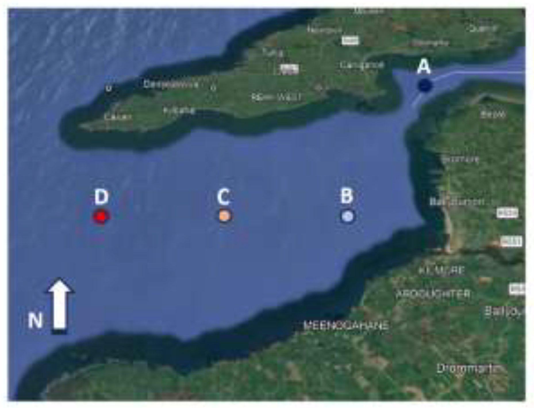
Figure 2.
Comparative analysis of the AMSSS at the points A, B, C, and D in the outer part of the estuary.
Figure 2.
Comparative analysis of the AMSSS at the points A, B, C, and D in the outer part of the estuary.
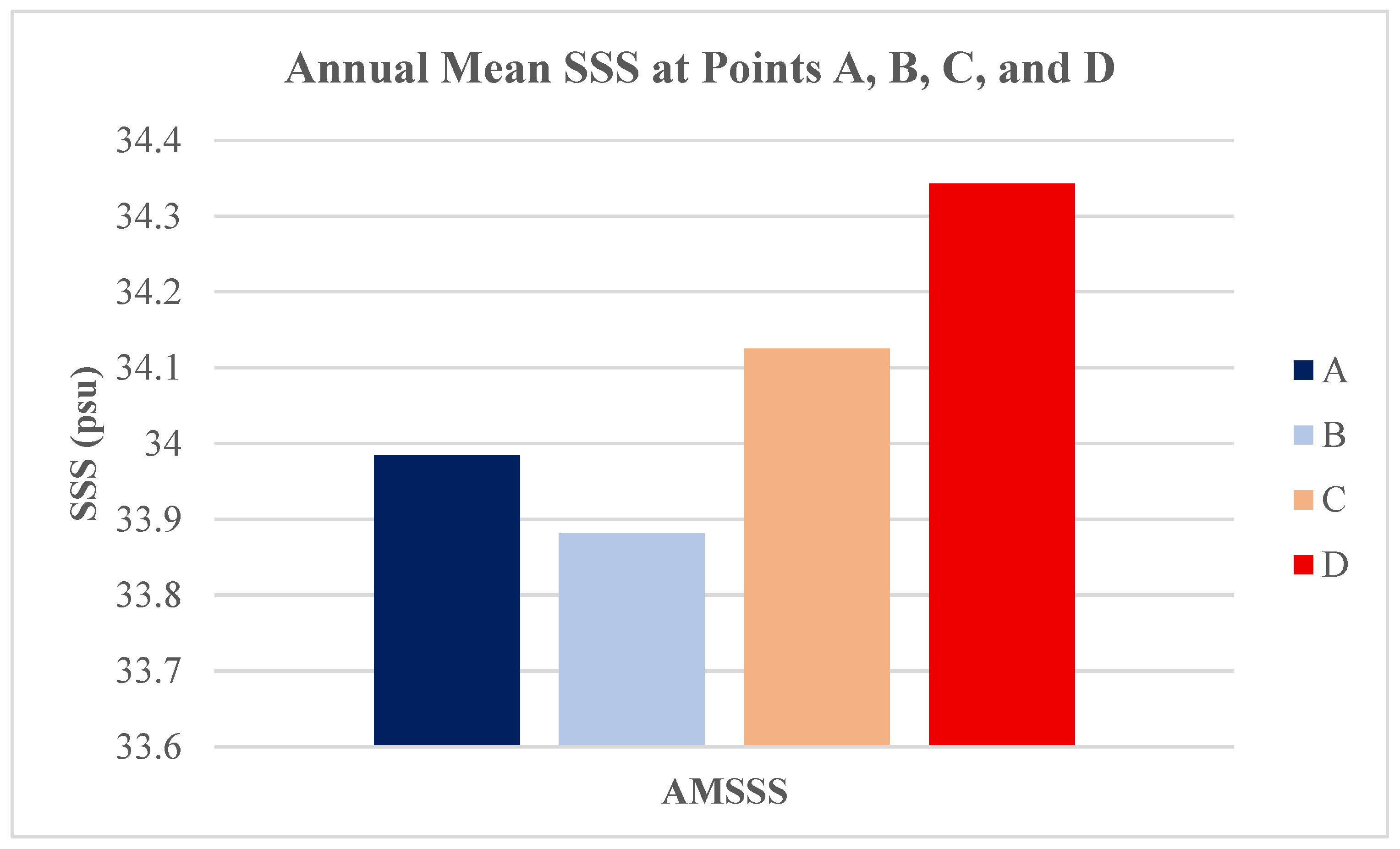
Figure 3.
Comparative analysis of the AMCV at the points A, B, C, and D in the outer part of the estuary.
Figure 3.
Comparative analysis of the AMCV at the points A, B, C, and D in the outer part of the estuary.
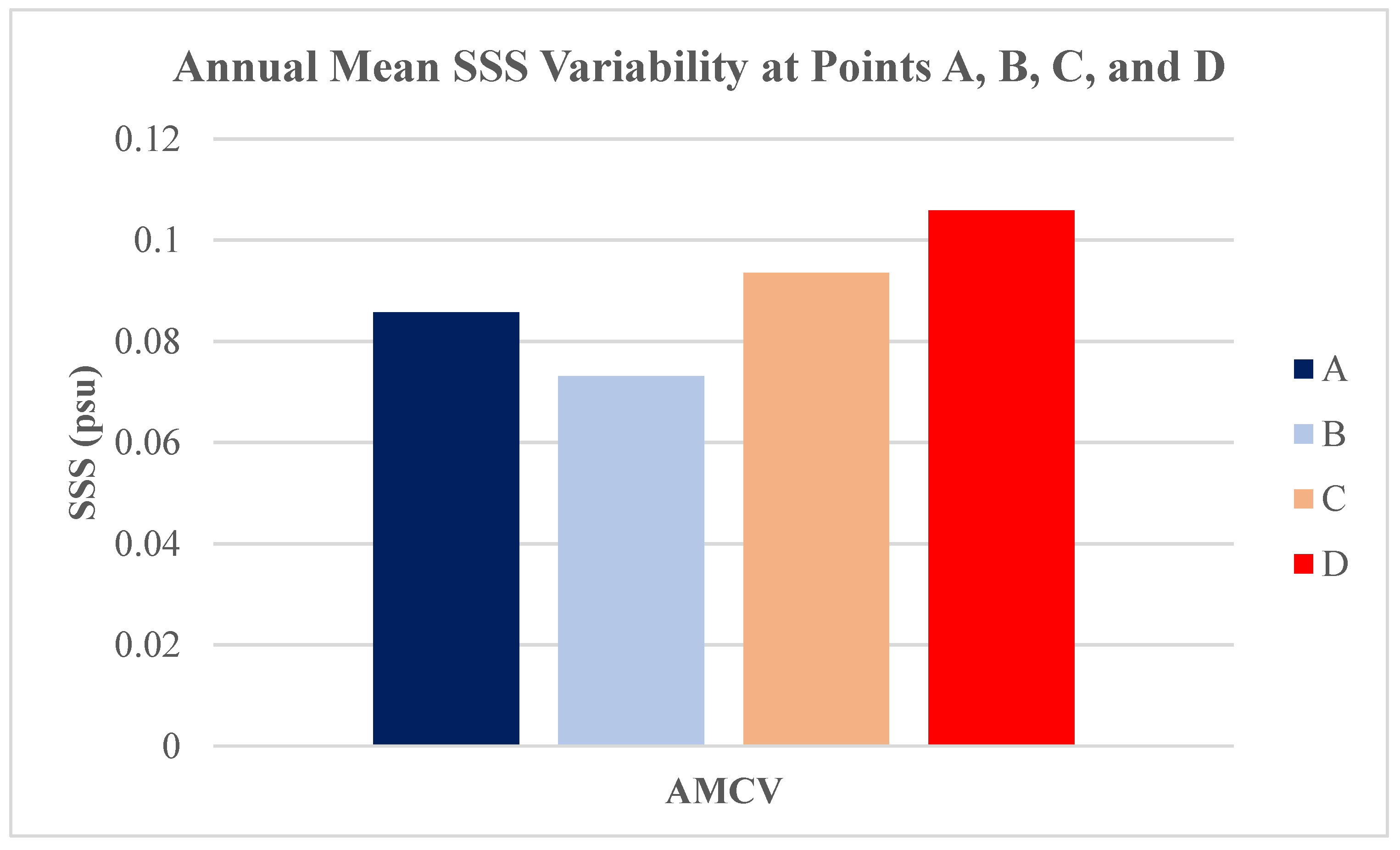

Table 1.
Daily mean SSS and measures of the SSS variability at the point A of the outer Sharon Estuary.
Table 1.
Daily mean SSS and measures of the SSS variability at the point A of the outer Sharon Estuary.
| Point A Samples | Season | Date | Mean (psu) | RG (psu) | SD (psu) | CV (%) |
|---|---|---|---|---|---|---|
| 1 | Spring | 01/03/2024 | 34.298715 | 0.162434 | 0.053891 | 0.157122 |
| 2 | 11/03/2024 | 34.510161 | 0.091526 | 0.030802 | 0.089254 | |
| 3 | 21/03/2024 | 34.510023 | 0.096130 | 0.036850 | 0.106782 | |
| 4 | 01/04/2024 | 34.492884 | 0.024624 | 0.008013 | 0.023232 | |
| 5 | 11/04/2024 | 34.618972 | 0.012700 | 0.003733 | 0.010783 | |
| 6 | 21/04/2024 | 34.784401 | 0.085637 | 0.022171 | 0.063739 | |
| 7 | 01/05/2024 | 34.427838 | 0.094940 | 0.033431 | 0.097104 | |
| 8 | 11/05/2024 | 33.503885 | 0.269230 | 0.092254 | 0.275353 | |
| 9 | 21/05/2024 | 33.428696 | 0.203966 | 0.076579 | 0.229081 | |
| 10 | Summer | 01/06/2024 | 33.702557 | 0.100656 | 0.028089 | 0.083345 |
| 11 | 11/06/2024 | 33.459394 | 0.094868 | 0.025515 | 0.076258 | |
| 12 | 21/06/2024 | 33.647339 | 0.028370 | 0.008548 | 0.025404 | |
| 13 | 01/07/2024 | 33.733879 | 0.053753 | 0.016953 | 0.050254 | |
| 14 | 11/07/2024 | 33.754330 | 0.068944 | 0.022329 | 0.066152 | |
| 15 | 21/07/2024 | 33.690990 | 0.017135 | 0.006680 | 0.019828 | |
| 16 | 01/08/2024 | 33.569761 | 0.052545 | 0.017699 | 0.052723 | |
| 17 | 11/08/2024 | 33.832907 | 0.165326 | 0.051926 | 0.153479 | |
| 18 | 21/08/2024 | 33.943738 | 0.060383 | 0.022142 | 0.065232 | |
| 19 | Autumn | 01/09/2024 | 34.122872 | 0.104625 | 0.039945 | 0.117061 |
| 20 | 11/09/2024 | 34.487670 | 0.104797 | 0.033901 | 0.098300 | |
| 21 | 21/09/2024 | 34.182195 | 0.023360 | 0.008058 | 0.023573 | |
| 22 | 01/10/2024 | 34.567840 | 0.053322 | 0.015604 | 0.045141 | |
| 23 | 11/10/2024 | 34.556518 | 0.086578 | 0.032120 | 0.092949 | |
| 24 | 21/10/2024 | 34.136005 | 0.019686 | 0.006339 | 0.018569 | |
| 25 | 01/11/2024 | 33.745617 | 0.163037 | 0.049891 | 0.147846 | |
| 26 | 11/11/2024 | 33.675486 | 0.089143 | 0.027903 | 0.082858 | |
| 27 | 21/11/2024 | 33.684520 | 0.158216 | 0.051359 | 0.152471 | |
| 28 | Winter | 01/12/2024 | 33.796860 | 0.044574 | 0.012558 | 0.037158 |
| 29 | 11/12/2024 | 34.318029 | 0.005717 | 0.001371 | 0.003996 | |
| 30 | 21/12/2024 | 33.720513 | 0.085600 | 0.026028 | 0.077186 | |
| 31 | 01/01/2025 | 33.667395 | 0.036430 | 0.009626 | 0.028591 | |
| 32 | 11/01/2025 | 33.684627 | 0.136037 | 0.049806 | 0.147859 | |
| 33 | 21/01/2025 | 33.263567 | 0.080543 | 0.026291 | 0.079038 | |
| 34 | 01/02/2025 | 33.649305 | 0.178796 | 0.054306 | 0.161388 | |
| 35 | 11/02/2025 | 34.288933 | 0.080297 | 0.025662 | 0.074841 | |
| 36 | 21/02/2025 | 33.983819 | 0.051148 | 0.017570 | 0.051700 |
Table 2.
Daily mean SSS and measures of the SSS variability at the point B of the outer Sharon Estuary.
Table 2.
Daily mean SSS and measures of the SSS variability at the point B of the outer Sharon Estuary.
| Point B Samples | Season | Date | Mean (psu) | RG (psu) | SD (psu) | CV (%) |
|---|---|---|---|---|---|---|
| 1 | Spring | 01/03/2024 | 34.237736 | 0.014852 | 0.004392 | 0.012827 |
| 2 | 11/03/2024 | 34.335301 | 0.060710 | 0.021401 | 0.062331 | |
| 3 | 21/03/2024 | 34.448374 | 0.005767 | 0.001893 | 0.005496 | |
| 4 | 01/04/2024 | 34.436681 | 0.058387 | 0.021443 | 0.062268 | |
| 5 | 11/04/2024 | 34.648511 | 0.015695 | 0.004893 | 0.014123 | |
| 6 | 21/04/2024 | 34.673115 | 0.058434 | 0.015315 | 0.044170 | |
| 7 | 01/05/2024 | 34.323199 | 0.060223 | 0.021250 | 0.061912 | |
| 8 | 11/05/2024 | 33.310454 | 0.219147 | 0.084172 | 0.252689 | |
| 9 | 21/05/2024 | 33.111562 | 0.105160 | 0.041184 | 0.124379 | |
| 10 | Summer | 01/06/2024 | 33.494616 | 0.069672 | 0.022903 | 0.068377 |
| 11 | 11/06/2024 | 33.252197 | 0.099080 | 0.026565 | 0.079889 | |
| 12 | 21/06/2024 | 33.431608 | 0.093653 | 0.031963 | 0.095608 | |
| 13 | 01/07/2024 | 33.474577 | 0.031353 | 0.009839 | 0.029393 | |
| 14 | 11/07/2024 | 33.572949 | 0.081225 | 0.029819 | 0.088820 | |
| 15 | 21/07/2024 | 33.707322 | 0.031819 | 0.010681 | 0.031687 | |
| 16 | 01/08/2024 | 33.550655 | 0.041168 | 0.014429 | 0.043008 | |
| 17 | 11/08/2024 | 33.747678 | 0.079597 | 0.024258 | 0.071880 | |
| 18 | 21/08/2024 | 34.059983 | 0.144222 | 0.045329 | 0.133087 | |
| 19 | Autumn | 01/09/2024 | 34.076510 | 0.147698 | 0.054931 | 0.161198 |
| 20 | 11/09/2024 | 34.297628 | 0.058705 | 0.018773 | 0.054735 | |
| 21 | 21/09/2024 | 34.115215 | 0.041970 | 0.012886 | 0.037771 | |
| 22 | 01/10/2024 | 34.360936 | 0.040477 | 0.011001 | 0.032017 | |
| 23 | 11/10/2024 | 34.339218 | 0.068001 | 0.024438 | 0.071165 | |
| 24 | 21/10/2024 | 34.285179 | 0.049433 | 0.015242 | 0.044456 | |
| 25 | 01/11/2024 | 33.540453 | 0.122115 | 0.035275 | 0.105170 | |
| 26 | 11/11/2024 | 33.622662 | 0.132102 | 0.044071 | 0.131075 | |
| 27 | 21/11/2024 | 33.518069 | 0.017990 | 0.005920 | 0.017661 | |
| 28 | Winter | 01/12/2024 | 33.874887 | 0.016799 | 0.005187 | 0.015313 |
| 29 | 11/12/2024 | 34.099960 | 0.015604 | 0.004215 | 0.012361 | |
| 30 | 21/12/2024 | 33.818306 | 0.104851 | 0.033870 | 0.100153 | |
| 31 | 01/01/2025 | 33.830908 | 0.017415 | 0.006878 | 0.020329 | |
| 32 | 11/01/2025 | 33.451529 | 0.188507 | 0.073560 | 0.219899 | |
| 33 | 21/01/2025 | 33.111742 | 0.127147 | 0.039075 | 0.118011 | |
| 34 | 01/02/2025 | 33.494529 | 0.025875 | 0.007285 | 0.021751 | |
| 35 | 11/02/2025 | 33.919570 | 0.079586 | 0.024815 | 0.073158 | |
| 36 | 21/02/2025 | 34.143301 | 0.114468 | 0.038059 | 0.111468 |
Table 3.
Daily mean SSS and measures of the SSS variability at the point C of the outer Sharon Estuary.
Table 3.
Daily mean SSS and measures of the SSS variability at the point C of the outer Sharon Estuary.
| Point C Samples | Season | Date | Mean (psu) | RG (psu) | SD (psu) | CV (%) |
|---|---|---|---|---|---|---|
| 1 | Spring | 01/03/2024 | 34.563053 | 0.018589 | 0.005016 | 0.014514 |
| 2 | 11/03/2024 | 34.499021 | 0.077318 | 0.025138 | 0.072865 | |
| 3 | 21/03/2024 | 34.648207 | 0.079105 | 0.027410 | 0.079109 | |
| 4 | 01/04/2024 | 34.540096 | 0.101696 | 0.034875 | 0.100969 | |
| 5 | 11/04/2024 | 34.784297 | 0.027610 | 0.008029 | 0.023082 | |
| 6 | 21/04/2024 | 34.681515 | 0.099289 | 0.028590 | 0.082435 | |
| 7 | 01/05/2024 | 34.376874 | 0.085750 | 0.031917 | 0.092844 | |
| 8 | 11/05/2024 | 33.347330 | 0.150795 | 0.061610 | 0.184753 | |
| 9 | 21/05/2024 | 33.191594 | 0.080250 | 0.028950 | 0.087220 | |
| 10 | Summer | 01/06/2024 | 33.773808 | 0.118670 | 0.033438 | 0.099004 |
| 11 | 11/06/2024 | 33.489533 | 0.194882 | 0.047876 | 0.142959 | |
| 12 | 21/06/2024 | 33.873086 | 0.046272 | 0.013320 | 0.039323 | |
| 13 | 01/07/2024 | 33.854334 | 0.049549 | 0.013925 | 0.041132 | |
| 14 | 11/07/2024 | 33.953983 | 0.097290 | 0.039166 | 0.115351 | |
| 15 | 21/07/2024 | 33.977299 | 0.046404 | 0.015277 | 0.044963 | |
| 16 | 01/08/2024 | 33.728496 | 0.080226 | 0.029375 | 0.087092 | |
| 17 | 11/08/2024 | 34.039273 | 0.151350 | 0.051449 | 0.151146 | |
| 18 | 21/08/2024 | 34.391813 | 0.099296 | 0.031870 | 0.092669 | |
| 19 | Autumn | 01/09/2024 | 34.191468 | 0.239971 | 0.088144 | 0.257796 |
| 20 | 11/09/2024 | 34.594472 | 0.009865 | 0.003258 | 0.009418 | |
| 21 | 21/09/2024 | 34.218423 | 0.059490 | 0.015366 | 0.044905 | |
| 22 | 01/10/2024 | 34.572060 | 0.121262 | 0.037416 | 0.108227 | |
| 23 | 11/10/2024 | 34.523812 | 0.076677 | 0.027857 | 0.080688 | |
| 24 | 21/10/2024 | 34.502391 | 0.041149 | 0.012563 | 0.036412 | |
| 25 | 01/11/2024 | 33.672336 | 0.157406 | 0.043548 | 0.129327 | |
| 26 | 11/11/2024 | 33.813378 | 0.223892 | 0.076409 | 0.225972 | |
| 27 | 21/11/2024 | 33.934406 | 0.089990 | 0.032494 | 0.095755 | |
| 28 | Winter | 01/12/2024 | 34.394795 | 0.038790 | 0.010389 | 0.030204 |
| 29 | 11/12/2024 | 34.251262 | 0.016260 | 0.004821 | 0.014077 | |
| 30 | 21/12/2024 | 34.120991 | 0.050763 | 0.016399 | 0.048062 | |
| 31 | 01/01/2025 | 34.172597 | 0.017877 | 0.004291 | 0.012557 | |
| 32 | 11/01/2025 | 33.760545 | 0.222544 | 0.090221 | 0.267237 | |
| 33 | 21/01/2025 | 33.378036 | 0.193153 | 0.057760 | 0.173049 | |
| 34 | 01/02/2025 | 33.894798 | 0.143806 | 0.043128 | 0.127241 | |
| 35 | 11/02/2025 | 34.239221 | 0.104046 | 0.034260 | 0.100062 | |
| 36 | 21/02/2025 | 34.559765 | 0.052101 | 0.018507 | 0.053551 |
Table 4.
Daily mean SSS and measures of the SSS variability at the point D of the outer Sharon Estuary.
Table 4.
Daily mean SSS and measures of the SSS variability at the point D of the outer Sharon Estuary.
| Point D Samples | Season | Date | Mean (psu) | RG (psu) | SD (psu) | CV (%) |
|---|---|---|---|---|---|---|
| 1 | Spring | 01/03/2024 | 34.751702 | 0.034303 | 0.011495 | 0.033076 |
| 2 | 11/03/2024 | 34.670959 | 0.113103 | 0.027007 | 0.077896 | |
| 3 | 21/03/2024 | 34.795253 | 0.164240 | 0.055321 | 0.158991 | |
| 4 | 01/04/2024 | 34.655781 | 0.098129 | 0.038435 | 0.110906 | |
| 5 | 11/04/2024 | 34.900583 | 0.051796 | 0.015119 | 0.043321 | |
| 6 | 21/04/2024 | 34.762421 | 0.095762 | 0.025016 | 0.071962 | |
| 7 | 01/05/2024 | 34.495850 | 0.123470 | 0.046984 | 0.136202 | |
| 8 | 11/05/2024 | 33.519871 | 0.169124 | 0.050827 | 0.151634 | |
| 9 | 21/05/2024 | 33.236317 | 0.102910 | 0.027724 | 0.083414 | |
| 10 | Summer | 01/06/2024 | 34.056611 | 0.127343 | 0.031153 | 0.091474 |
| 11 | 11/06/2024 | 33.790268 | 0.242560 | 0.074704 | 0.221080 | |
| 12 | 21/06/2024 | 34.243342 | 0.040696 | 0.012181 | 0.035571 | |
| 13 | 01/07/2024 | 34.130994 | 0.066400 | 0.021533 | 0.063091 | |
| 14 | 11/07/2024 | 34.463487 | 0.241383 | 0.075468 | 0.218981 | |
| 15 | 21/07/2024 | 34.115649 | 0.044231 | 0.014258 | 0.041794 | |
| 16 | 01/08/2024 | 33.918320 | 0.109015 | 0.035671 | 0.105167 | |
| 17 | 11/08/2024 | 34.369210 | 0.117451 | 0.039373 | 0.114560 | |
| 18 | 21/08/2024 | 34.626798 | 0.023023 | 0.007611 | 0.021980 | |
| 19 | Autumn | 01/09/2024 | 34.432696 | 0.291896 | 0.109648 | 0.318442 |
| 20 | 11/09/2024 | 34.769193 | 0.066945 | 0.022024 | 0.063344 | |
| 21 | 21/09/2024 | 34.400365 | 0.059494 | 0.017002 | 0.049424 | |
| 22 | 01/10/2024 | 34.822076 | 0.073953 | 0.020474 | 0.058797 | |
| 23 | 11/10/2024 | 34.629112 | 0.059774 | 0.022345 | 0.064526 | |
| 24 | 21/10/2024 | 34.663815 | 0.066402 | 0.019529 | 0.056338 | |
| 25 | 01/11/2024 | 33.976872 | 0.256877 | 0.073987 | 0.217756 | |
| 26 | 11/11/2024 | 34.142424 | 0.229914 | 0.079239 | 0.232084 | |
| 27 | 21/11/2024 | 34.224360 | 0.112740 | 0.039765 | 0.116190 | |
| 28 | Winter | 01/12/2024 | 34.672275 | 0.027300 | 0.007434 | 0.021442 |
| 29 | 11/12/2024 | 34.298752 | 0.022072 | 0.008282 | 0.024146 | |
| 30 | 21/12/2024 | 34.297684 | 0.037726 | 0.010866 | 0.031681 | |
| 31 | 01/01/2025 | 34.412212 | 0.060174 | 0.019736 | 0.057352 | |
| 32 | 11/01/2025 | 34.053443 | 0.178782 | 0.075560 | 0.221886 | |
| 33 | 21/01/2025 | 33.781763 | 0.201099 | 0.060514 | 0.179132 | |
| 34 | 01/02/2025 | 34.198282 | 0.142920 | 0.044243 | 0.129372 | |
| 35 | 11/02/2025 | 34.280352 | 0.153214 | 0.049099 | 0.143227 | |
| 36 | 21/02/2025 | 34.782028 | 0.048710 | 0.015718 | 0.045190 |
Table 5.
Statistical significance of the difference in the SSS hourly variability at various points.
Table 5.
Statistical significance of the difference in the SSS hourly variability at various points.
| SSS Points | F-value | P-value | P-value Interpretation | SD Value | Direction of the Variability Difference Based on the SD |
|---|---|---|---|---|---|
| A vs B | 4.7497 | 0.0294 | Statistically significant | 0.4075 vs 0.4330 | Variability at point A < point B |
| A vs C | 0.0611 | 0.8047 | Not statistically significant | 0.4075 vs 0.4135 | Variability at point A < point C |
| A vs D | 12.9810 | 0.0003 | Statistically significant | 0.4075 vs 0.3854 | Variability at point A > point D |
| B vs C | 7.1914 | 0.0074 | Statistically significant | 0.4330 vs 0.4135 | Variability at point B > point C |
| B vs D | 41.5310 | 0.0000 | Statistically significant | 0.4330 vs 0.3854 | Variability at point B > point D |
| C vs D | 13.5070 | 0.0003 | Statistically significant | 0.4135 vs 0.3854 | Variability at point C > point D |
Disclaimer/Publisher’s Note: The statements, opinions and data contained in all publications are solely those of the individual author(s) and contributor(s) and not of MDPI and/or the editor(s). MDPI and/or the editor(s) disclaim responsibility for any injury to people or property resulting from any ideas, methods, instructions or products referred to in the content. |
© 2026 by the authors. Licensee MDPI, Basel, Switzerland. This article is an open access article distributed under the terms and conditions of the Creative Commons Attribution (CC BY) license (http://creativecommons.org/licenses/by/4.0/).
Copyright: This open access article is published under a Creative Commons CC BY 4.0 license, which permit the free download, distribution, and reuse, provided that the author and preprint are cited in any reuse.


