Submitted:
12 January 2026
Posted:
13 January 2026
You are already at the latest version
Abstract
This study introduces a novel neural network-based symbolic computation algorithm (NNSCA) for obtaining exact solutions to the (3+1)dimension Jimbo-Miwa equation. By integrating neural networks with symbolic computation, NNSCA addresses the limitations of conventional approaches, enabling the derivation and visualization of exact solutions. The neural network architecture is meticulously designed, and the partial differential equation is transformed into algebraic constraints via Maple, establishing a closed-loop solution framework. NNSCA offers a generalized paradigm for investigating high-dimensional nonlinear partial differential equations, highlighting its substantial application prospects.
Keywords:
(3+1)dimension Jimbo-Miwa equation
; neural network-based symbolic computation algorithm
; exact solution
; neural network
; symbolic computation
; nonlinear partial differential equation
1. Introduction
Nonlinear partial differential equations (NLPDEs) provide indispensable mathematical frameworks for modeling complex phenomena across diverse scientific and engineering domains, including biology (Wang 2024), quantum mechanics (Yel 2017), financial mathematics (Rrey 2011), fluid mechanics (Xu 2024), optics (Arnous 2022), and plasma physics (Song 2023). Their capacity to accurately capture intricate system behaviors underpins critical applications, exemplified by the Navier-Stokes equations in aerospace engineering (Lin 2017) and meteorological forecasting (Melet 2020).
Among integrable NLPDEs of significant theoretical and applied interest is the Jimbo-Miwa equation, originally introduced by Jimbo and Miwa(Jimbo 1983). This equation finds broad relevance within mathematical and theoretical physics. Its (3+1)-dimensional variant, defined across three spatial dimensions and one temporal dimension, offers a powerful model for investigating complex wave propagation and interaction dynamics in higher dimensions. The equation reads Eq.(1):
where u(x, y, z, t) represents a potential function, often interpreted physically as the amplitude or field evolution potential of a high-dimensional nonlinear wave. The structure of Eq. (1) reveals key dynamical components: The terms constitute the nonlinearity, driving waveform distortion through self-modulation. The fourth-order mixed derivative acts as a higher-order dispersion term, counteracting nonlinear effects to enable stable structures like solitons. The cross-derivative terms introduce multidimensional coupling, constraining the wave evolution across space-time and enabling the existence of localized lumps, oblique waves, and genuine (3+1)dimension solitons.Consequently, the (3+1)dimension Jimbo-Miwa equation serves as a cornerstone model for exploring intricate three-dimensional nonlinear wave phenomena, particularly in plasma physics(Xu 2023; Yan 2019; Dhiman 2021)
The quest for exact solutions to the Jimbo-Miwa equation solitons (Liu 2023; Seadawy 2022), breathers(Guo 2020; Zhang 2017), rogue waves (Liu 2019; Srivastava 2024), lumps and their interactions (Yan 2018),remains a vibrant area of research. Such solutions provide profound insights into nonlinear wave dynamics and underpin theoretical advances in NLPDEs, while also offering mathematical foundations for understanding complex physical systems (Tang 2021). Numerous analytical techniques have been deployed to tackle this equation. These include: Hirota’s bilinear method, used to systematically derive lump and lump-like solutions via Bell polynomials (Su 2012).The (G’/G)-expansion method and its variants, yielding traveling wave solutions expressed through hyperbolic, trigonometric, and rational functions (Song 2010; Sirisubtawee 2017).Bell polynomial schemes combined with Bäcklund transformations, Lax pairs, and the three-wave method for constructing bilinear forms and periodic waves (Liu 2019).Test function approaches aided by symbolic computation for finding solitary wave solutions (Singh 2015; Yan 2003).
Nevertheless, significant challenges persist. The efficacy of these methods often depends heavily on the specific equation structure or the anticipated solution form (e.g., traveling vs. non-traveling waves, solutions with arbitrary functions) (Shen 2025). Crucially, transforming a given NLPDE into the Hirota bilinear form—a powerful route to exact solutions—is not always feasible, limiting applicability. Even when successful, the resulting bilinear system for high-dimensional or complex NLPDEs can involve intricate symbolic computations, especially when constructing solutions with numerous parameters (e.g., ensuring analyticity for a 15-parameter lump solution (Yong 2018)). This computational burden underscores the need for more robust and efficient methods for deriving exact solutions.
Recent advances in neural networks (NNs) offer promising new paradigms for solving NLPDEs. The theoretical foundation, established by the Universal Approximation Theorem (Cybenko 1989), guarantees that NNs can approximate complex continuous functions. Physics-Informed Neural Networks (PINNs)(Raissi 2019)embed PDE residuals directly into the loss function, enabling solution discovery even with sparse data. Building on this, the Bilinear Neural Network Method (BNNM) (Zhang 2019)represents a significant innovation. BNNM synergizes the expressive power of neural networks with the analytical structure of Hirota’s bilinear form, efficiently generating exact analytical solutions—such as solitons, breathers, and rogue waves—critical to fields like optics and fluid mechanics. BNNM has demonstrated notable success in solving various NLPDEs, yielding breathers and interacting solitons for the (2+1)D Hirota-Satsuma-Ito equation (Zhu 2023), novel test functions and rogue waves for generalized breaking wave equations (Zhang 2022), periodic solitons for the (3+1)-dimensional Boiti–Leon–Manna–Pempinelli(BLMP) equation (Shen 2021), lump and bright-dark soliton solutions for the (3+1)-dimensional Geng equation (Lei 2024), and M-lump and lump-breather solutions for the KP-BBM equation (Huang 2024).
Inspired by the BNNM yet addressing its limitations, this study introduces the Neural Network Symbolic Computation Algorithm NNSCA. NNSCA derives exact solutions for the (3+1)dimension Jimbo-Miwa equation. It achieves deeper integration through three mechanisms: incorporating symbolic priors from mathematical structures, utilizing neural networks’ multidimensional approximation capabilities, and enforcing complementary logic. This framework combines symbolic rigor with efficient solution space exploration. It effectively bridges symbolic computation and data-driven approaches. NNSCA demonstrates key advantages. It reduces structural dependence on specific equation forms. The method mitigates overfitting risks common in purely data-driven high-dimensional systems. It enables automated discovery of analytical solutions without manual hypothesis. Computational efficiency improves dramatically: parameter-constrained equation systems automate solution derivation, compressing weeks of manual effort to minutes. Applying NNSCA to the (3+1)dimension Jimbo-Miwa equation, we achieve the first automated discovery of diverse analytical solutions—including solitons, lumps, and periodic waves. Subsequent visualization via 3D surfaces, spacetime slices, and high-dimensional projections elucidates key dynamical features such as wave localization, periodicity, and intricate multidimensional coupling mechanisms.
The remainder of this paper is structured as follows: Section 2 details the foundational principles and procedural steps of the NNSCA for solving NLPDEs. Section 3 demonstrates the method’s application to the (3+1)dimension Jimbo-Miwa equation using single-hidden-layer neural network models, presenting analytical solutions derived from two distinct coefficient sets alongside visualizations. Section 4 enhances model complexity with a two-hidden-layer architecture, solving the same equation and illustrating results using two further coefficient sets. Finally, Section 5 concludes the study.
2. Principles of Neural Network Based Symbolic Algorithm (NNSCA)
This study mainly uses NNSCA to solve the analytical solution of the (3+1)dimension Jimbo-Miwa equation and visualise its analytical solution. The specific solution structure of NNSCA is shown in Figure 1.
Step 1:Building a high-dimensional neural network architecture. Construct a multi-layer perceptron architecture adapted to (3+1) spatial-temporal dimensions, with the input layer connected to independent variables to capture four-dimensional coupling effects; The hidden layer uses a customised family of activation functions that combine hyperbolic, trigonometric, and exponential functions to adapt to the local and periodic characteristics of high-dimensional waves, breaking through the traditional symbolic method’s assumption of solution forms and adaptively exploring the complex solution space containing solitons, lumps, and periodic waves; The output layer directly defines the probe function , leveraging the degrees of freedom of network weights and biases to pre-construct the expression form of high-dimensional solutions.
Step 2: Symbolic derivation of partial derivatives of all orders. Using the Maple symbolic computation engine, perform a full-order partial derivative expansion of the output f, covering all derivative terms involved in the (3+1)dimension Jimbo-Miwa equation. Recursively process composite operations using the chain rule to strictly ensure the mathematical rigour of the differential derivation, avoiding numerical differentiation truncation errors, and providing accurate derivative support for subsequent equation substitution.
Step 3: Symbolic Mapping of the Target PDE. Substitute the partial derivatives of f into the (3+1)-dimensional Jimbo-Miwa equation. Through algebraic operations such as rationalisation and combining like terms, gradually eliminate terms directly associated with the unknown solution, transforming it into an equation containing only f and its partial derivatives, neural network weights, and biases. This process achieves a dimensionality reduction mapping from partial differential constraints to algebraic constraints, transforming the infinite-dimensional function constraints of the high-dimensional PDE into finite-dimensional algebraic constraints on the network parameters.
Step 4: Construction of the parameter constraint equation system. For the transformed equations, group terms by spatial-temporal variable powers and neural network parameters, and use the ‘like-term collection’ feature of symbolic computation to extract the coefficient functions for each group of terms. Force all coefficients to zero to ensure the validity of the PDE, generating an algebraic constraint equation system for neural network weights and biases. Compress the parameter space through sparsification processing, constraining the range of free parameters in the neural network to the subspace satisfying the PDE solution.
Step 5: Symbolic solution and constraint screening. Call the Maple symbolic solver to analyse the constraint system of equations and address the challenge of nonlinear multi-solution: combine the physical constraints and mathematical constraints of the (3+1)dimension Jimbo-Miwa equation to screen for valid solutions, obtain parameter analytical relationships or specific parameter values, and establish a mapping between network parameters and high-dimensional wave physical quantities.
Step 6: Constraint Back-Substitution and Closed-Loop Verification. Substitute the obtained parameters back into the initial probe function f to reconstruct the exact probe function f that satisfies the PDE constraints. Conduct symbolic verification by substituting into the (3+1)dimension Jimbo-Miwa equation, i.e., use Maple to recalculate the derivatives and verify the validity of the equation, forming a closed-loop process from neural network pre-exploration to symbolic constraint derivation, parameter solution, and final back-substitution verification, ultimately outputting a (3+1)dimension analytical solution that strictly satisfies the equation.
3. Single layer
3.1. Model [4-3-1]-1
To solve the (3+1)dimension Jimbo-Miwa equation (1), we designed a single-layer neural network model diagram based on the characteristics of the equation, as shown in Figure 2a. This single-layer neural network model diagram is model [4-3-1], where the input layer has four neurons, namely x, y, z, and t, the hidden layer has three neurons , , and , and the output layer is the output probe function .
Now, based on the single-layer neural network model diagram(Figure 2) we construct the activation functions. We set the activation function , , and , resulting in the model shown in Figure 2b. [4-3-1]-1. By outputting the neural network model, we obtain the test function (2)
Differentiate the test function (2) and substitute it back into (1) to obtain a more complex equation. Collect the coefficients of each term to obtain the corresponding underdetermined nonlinear algebraic equation system. Use Maple to solve this equation system and obtain two sets of coefficient solutions, Case 1 and Case 2, as shown in (3) and (4), respectively.
For Case 1, we substitute (3) into (2) and simplify to obtain the analytical solution of the (3+1)dimension Jimbo-Miwa equation as shown in (5).
To confirm the accuracy of the solution in equation (5), we insert the analytical solution into the left-hand side of the (3+1)dimension Jimbo-Miwa equation (1) and employ Maple software to streamline the outcome. The process reveals that the left-hand side of equation (1) consistently equals zero. This demonstrates that the analytical solution (5) is both precise and error-free, while also underscoring the superiority of this approach compared to traditional numerical techniques. To briefly analyse its dynamic characteristics, we now visualise the analytical solution obtained, taking the corresponding parameters , , , , , , , , , , , , , , , , , , , . The spatiotemporal dynamical visualisation of the analytical solution of the (3+1)dimension dimensional Jimbo-Miwa equation is shown in Figure 3a–d.
Three-dimensional graphs (Figure 3a) visually present the spatiotemporal evolution of the solutions to the (3+1)dimension Jimbo-Miwa equation on the x-t plane amplitude surface: the undulating morphology of the surface reveals the quasi-periodic oscillation characteristics of nonlinear waves, and the extension direction of the wave peaks suggests a tendency for bidirectional propagation along the x axis; while the periodic folds of the surface reflect the dynamic balance between dispersion effects and nonlinear effects in the equation, confirming the solution’s stable propagation in high-dimensional space. In the contour diagrams (Figure3b), the red closed contours outline the localised distribution of high-amplitude wave packets, with their curved contours and nested structures suggesting that the waves propagate at non-uniform speeds; The periodic stripes on the blue background correspond to low-amplitude regions, reflecting the complex superposition effects of multi-directional wave interference in a (3+1)dimension system, highlighting the coupled characteristics of nonlinear waves localised oscillations–global periodic modulation. The thermal map (Figure3c) clearly reveals the multi-scale, quasi-periodic spatiotemporal dynamics captured by the neural network. This distinctive combination of periodicity and localized enhancement is a hallmark of modulational instability or the formation of breather lattices commonly observed in high-dimensional nonlinear wave equations.The periodic component, arising from the sinusoidal and cosinusoidal terms in the expression, imposes a regular grid-like modulation across the plane. Superimposed on this background, the envelope induces strong spatial localization, concentrating energy into isolated high-amplitude hotspots within each periodic cell. Such patterns closely resemble the quasi-periodic breather arrays or modulationally unstable structures that emerge in integrable or near-integrable systems, including higher-dimensional extensions of the nonlinear Schrödinger family and related soliton-bearing equations. These features underscore the model’s ability to faithfully reproduce complex, emergent nonlinear phenomena characteristic of the (3+1)dimensionimension Jimbo-Miwa equation. The evolution plot(Figure 3d) Select the x cross-sectional curves at five time points to clearly verify the bidirectional propagation law of the wave: when , the wave crest moves in the positive direction of the x axis, and when , it moves in the negative direction; The oscillation frequencies of the curves at each time point are similar, and the amplitude differences are stable, reflecting the shape conservation of the solution, while the localised distribution of the peaks highlights the energy aggregation effect dominated by nonlinearity.
For Case 2, if we substitute (4) into (2) and simplify, we obtain another analytical solution for the (3+1)dimensionimension Jimbo-Miwa equation, as shown in (6).
Likewise, to assess the dependability of the result in equation (6), we input the analytical solution of (6) into the left-hand side of the (3+1)dimension Jimbo-Miwa equation (1) and utilize Maple software to refine the outcome. The analysis confirms that the left-hand side of equation (1) consistently equals zero, suggesting that the analytical solution (6) is dependable Visualising the obtained analytical solution, we take the corresponding parameters , , , , , , , , , , , , , , , , , , , , , , , , , . The resulting spatiotemporal dynamical visualisation of the analytical solution to the (3+1)dimension Jimbo-Miwa equations is shown in Figure 4a–d.
This three-dimensional graph(Figure 4a) presents the spatiotemporal evolution of the solution to the (3+1)dimension Jimbo-Miwa equation in the form of an amplitude surface in the x-t plane: the spiral-like wrinkled morphology of the surface suggests a strong coupling between nonlinear and dispersion effects; wave crests extend along the composite direction of the x and t axes, reflecting the non-uniform propagation characteristics of waves in high-dimensional space; the periodic changes in colour gradients and height variations further confirm the quasi-periodic modulation patterns of the solutions. In the contour diagrams(Figure 4b), the red high-amplitude regions exhibit fragmented, non-closed distributions, breaking the regular contours of conventional localised wave packets, suggesting the disintegration and recombination of localised structures during wave propagation; The stripes in the background blue low-amplitude regions become more disordered, reflecting the enhanced non-uniformity of multi-directional wave interference within the (3+1)dimension system, highlighting the complexity of dynamic interactions under nonlinear effects in this group of solutions. Thermal maps(Figure 4c) depict the amplitude distribution in the x-t plane through colour gradients. High-amplitude patterns exhibit non-symmetric periodic arrangements, breaking the spatiotemporal symmetry of the first solution group and revealing its spatiotemporal symmetry-breaking characteristics; The ‘arc-shaped’ distribution of the colour gradient corresponds with the spiral trend in the three-dimensional plot, indirectly verifying the dynamical characteristics of wave propagation along the composite direction. The evolution profiles(Figure 4d) selecting the x cross-section curves at t = -20, -10, 0, 10, 20, it can be observed that the wave peaks propagate bidirectionally while accompanied by strong amplitude modulation: the central amplitude is highest at t = 0, and as time progresses, the amplitude difference between the two sides of the wave peaks significantly increases, reflecting the energy concentration effect dominated by nonlinearity; The enhanced difference in oscillation frequencies of the curves suggests dynamic changes in dispersion characteristics during propagation, further illustrating the multi-scale dynamical behaviour of the solutions to the (3+1)dimension Jimbo-Miwa equation.
3.2. Model [4-3-1]-2
To obtain different analytical solutions for neural network models with the same number of layers, we changed the activation functions in the hidden layers without changing the number of layers in the network model. We set the activation functions as , , , resulting in the model shown in Figure 2c [4-3-1]-2. By applying the output of the neural network model, we obtain the test function (7).
Differentiate the test function (7) and substitute it back into (1) to obtain a more complex equation. Collect the coefficients of each term to obtain the corresponding underdetermined nonlinear algebraic equation system. Use Maple to solve this equation system and obtain two sets of coefficient solutions, Case 1 and Case 2, as shown in (8) and (9), respectively.
For Case 1, we substitute (8) into (7) and simplify to obtain the analytical solution of the (3+1)dimension Jimbo-Miwa equation as shown in (10).
To validate the accuracy of the result in equation (8), we insert the analytical solution of (8) into the left-hand side of the (3+1)dimension Jimbo-Miwa equation (1) and apply Maple software to streamline the outcome. The analysis reveals that the left-hand side of equation (1) consistently equals zero, confirming that the analytical solution (8) is dependable and precise, with no error at this stage.
To visualise the obtained analytical solution, we take the corresponding parameters , , , , , , , , , , we obtain the spatiotemporal dynamical visualisation diagrams of the analytical solution shown in Figure 5a–d.
This three-dimensional graph(Figure 5a) shows a hyperbolic separation surface structure, with the amplitude sharply increasing at x=0. The surfaces on both sides rapidly decay along the x axis and extend along the t axis, revealing the strong localisation characteristics of the solution, i.e., the energy is highly concentrated in the narrow space-time region near x=0. The steep edges of the surface contrast sharply with the smooth transitions, reflecting the competitive mechanism between nonlinear localisation effects and dispersion diffusion in the (3+1)-dimensional Jimbo-Miwa equation, giving rise to shock-like localised wave structures. The contour lines are highly dense at x=0 and fan out in both directions along the t axis(Figure 5b). Combined with the colour scale, this visually demonstrates the line-localised distribution of energy; The extension trend of the lines confirms that while waves propagate bidirectionally along the t axis, localisation in the x direction continues to strengthen, highlighting the spatiotemporal constraint dynamics of localised waves in the (3+1)dimension system. In the thermal maps(Figure 5c), the bright strip running along the t axis at x=0 and the rapidly decaying colour gradients on both sides precisely depict the line localisation characteristics of the solution. The colour distribution is symmetric about x=0, verifying the spatial inversion symmetry of the solution and implying that the local structure maintains its morphological stability during propagation, further supporting the dominant role of nonlinear localisation. The evolution plot(Figure 5d) Selecting x cross-sectional curves at t = -20, -10, 0, 10, 20, it can be seen that a sharp peak always exists at x=0, with an amplitude far higher than on either side, and the peak position remains unchanged with t, with only a slight variation in the absolute value of the amplitude, reflecting the spatiotemporal locking characteristics of the localised structure; The consistency of the curve shapes confirms the strongly localised nature of the solutions to the (3+1)dimension Jimbo-Miwa equation, where energy is strictly confined to propagate within a low-dimensional subspace.
For Case 2, if we substitute (9) into (7) and simplify, we obtain another analytical solution for the (3+1)dimension Jimbo-Miwa equation, as shown in (11).
To confirm the trustworthiness of the result in equation (11), we integrate the analytical solution of (11) into the left-hand side of the (3+1)dimension Jimbo-Miwa equation (1) affirming that the analytical solution (8) no error. Visualising the obtained analytical solution, we take the corresponding parameters , , , , , , , , , , , , , , , , , , , , , resulting in the analytical solution’s spatiotemporal dynamics visualisation diagram shown in Figure 6a–d. To better illustrate the characteristics of three-dimensional graphs, their corresponding top-down views have been added.
In the three-dimensional graphs(Figure 6a) From a top-down perspective, the edges of the three-dimensional surface’s plateau exhibit sawtooth-like wrinkles, breaking the expectation of a perfectly flat top. This detail suggests that even within the localised region where energy is concentrated, quasi-periodic amplitude modulation still exists, reflecting the coexistence mechanism of localisation and modulation instability in high-dimensional systems, where nonlinearity dominates energy confinement and dispersion induces weak oscillations, jointly shaping the non-uniform local structure. The red closed contours outline arched localised regions, with the jagged edges of the contours corresponding to the wrinkles in the three-dimensional top-down view, verifying the quasi-periodic modulation within the localised regions(Figure 6b). The contour extends along the negative t axis to , suggesting a unidirectional propagation preference of the wave, revealing the asymmetric dynamical characteristics of the localised structure. In the thermal maps(Figure 6c), red arched bands are distributed along the ‘arched trajectory,’ with colours rapidly decaying from the centre to both sides, precisely delineating the spatiotemporal boundaries of the localised region; The arched vertices are located at and , and as t decreases, they spread out on both sides of the x axis, confirming the unique trajectory of the wave propagating along the arched path in the negative direction of the t axis, highlighting the non-trivial spatiotemporal evolution pattern of the (3+1)dimension solution. In the evolution plots (Figure 6d) Selecting x cross-section curves at t = -20, -10, 0, 10, 20, it can be seen that at , sharp minima appear at , while the central region maintains a stable high amplitude; As t deviates from 0, the sharpness of the valley decreases and the central amplitude slightly decays, reflecting the dynamic symmetry breaking of the localised structure, i.e., strict localisation only occurs near t = 0, and it gradually dissipates during propagation, revealing the time-dependent localisation characteristics of the (3+1)-dimensional Jimbo-Miwa equation solution.
4. Double Layer
4.1. Model [4-4-3-1]-1
To extract more solution sets from underdetermined systems of equations and reveal the rich dynamical properties of high-dimensional equations, we now increase the complexity of the model by constructing a neural network with two hidden layers to solve the (3+1)dimension Jimbo-Miwa equation. as shown in Figure 7a, which depicts the [4-4-3-1] two-layer hidden neural network model we have constructed. The input layer consists of four neurons, denoted as x, y, z, and t. The first hidden layer contains four neurons, denoted as , , , , the second hidden layer contains three neurons, represented as , , and , and the final output layer is the output probe function Now, we construct the activation function based on Figure 7a, , , , , , , , resulting in the model shown in Figure 7b [4-3-1]-1. By applying the output of the neural network model, we obtain the probe function (12).
Similar to the single hidden layer, differentiate and substitute back into (12) to obtain two coefficient solutions, Case 1 (13) and Case 2 (14), through NNSCA.
For the coefficient solution Case 1 (13), we substitute (13) into (12) and simplify it to obtain the analytical solution of the (3+1)dimension Jimbo-Miwa equation as shown in (15).
For the coefficient solution Case 1 (13), we substitute (13) into (12) and simplify it to obtain the analytical solution of the (3+1)dimension Jimbo-Miwa equation as shown in (15). Visualise the analytical solution obtained by setting the corresponding parameters , , , , , , , , , , , , , , , , , , , , , , , resulting in the analytical solution’s spatiotemporal dynamics visualisation diagram shown in Figure 8a, 8b, 8c and 8d.
The graph (Figure 8a) reveals highly consistent diagonal texture and color gradients across the three-dimensional surface. These patterns extend steadily along the direction. This confirms the wave’s strong preference for directional propagation. The dual-hidden-layer model captures this regular trajectory with precision. Deeper feature abstraction uncovers the underlying diagonal conservation law of the (3+1)dimension Jimbo-Miwa solution. In the contour diagram (Figure 8b), red closed vortices arrange periodically along the diagonal. Each vortex shows an amplitude difference exceeding 30 between center and edge. This highlights strong energy concentration in localized pulses. The wavy extension of blue outer lines resonates with the vortex period. It suggests a cyclic mechanism of pulse generation and annihilation. The pseudocolour thermal map (Figure 8c) displays red high-amplitude spots distributed at equal intervals along the diagonal. Strong contrast with the green background emphasizes the periodicity and isolation of the pulse trains. The narrow color scale indicates stable energy levels. Through complex feature transformations, the double-hidden-layer model reveals the periodic pulse flow pattern. This offers a fresh perspective on dynamic transport in high-dimensional systems. The evolution plots (Figure 8d) show x-profile curves at . Sharp peaks move linearly along the x-axis with time. Propagation occurs strictly along the direction. Peak amplitudes remain stable. Half-widths stay narrow. These features indicate motion-invariant solitons. The dual-hidden-layer architecture successfully extracts this directional periodic soliton solution from an underdetermined equation system. It demonstrates the model’s ability to reveal intricate dynamics in high-dimensional integrable equations.
For Case 2, we substitute (14) into (12) and simplify it to obtain another analytical solution for the (3+1)dimension Jimbo-Miwa equation, as shown in (16).
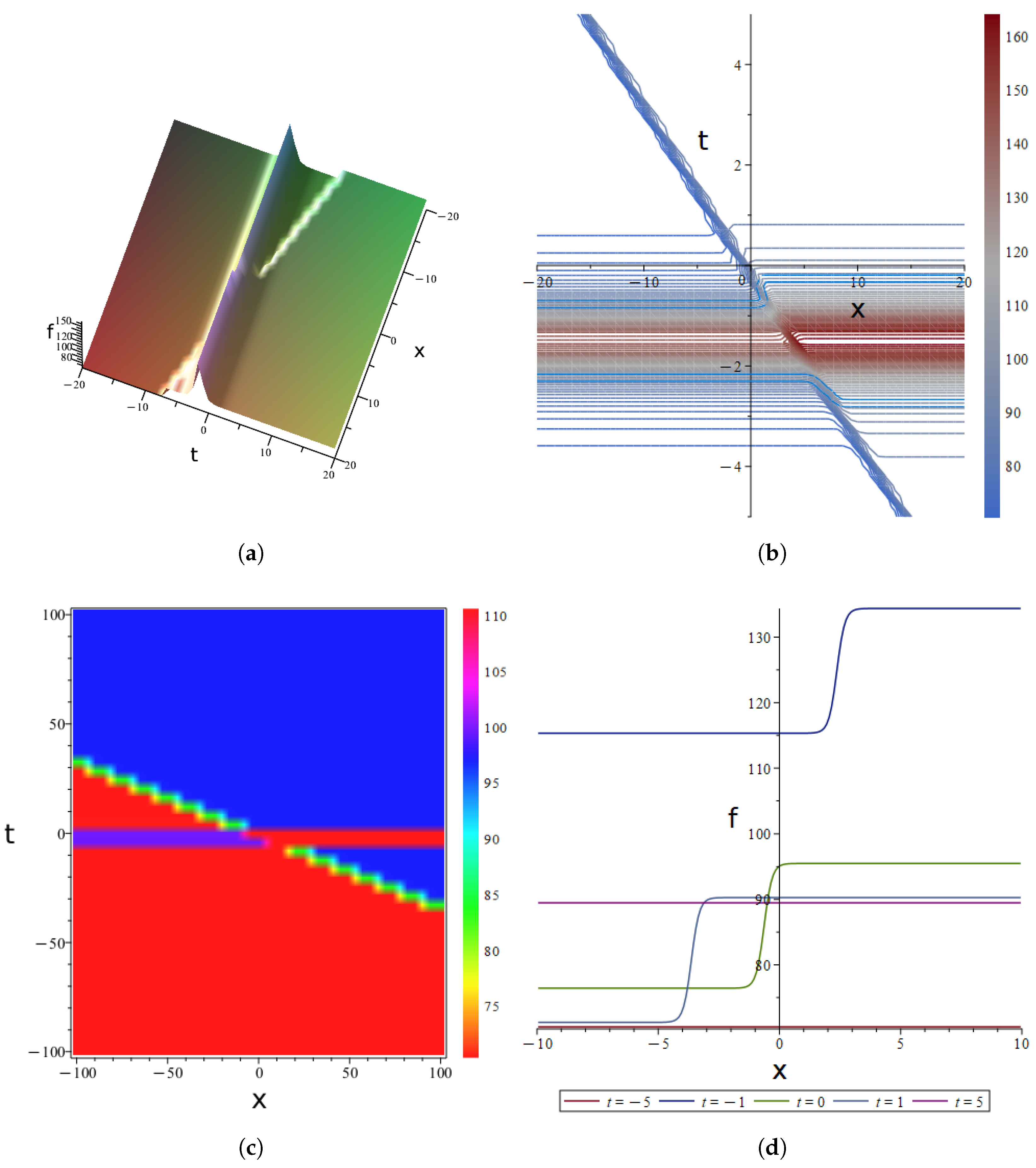
To verify the reliability of the result in (16), we substitute the analytical solution of (16) into the left side of the (3+1)dimension Jimbo-Miwa equation (1) under study and use Maple software to simplify the result, which shows that the left side of equation (1) is always equal to zero. This indicates that the neural network with two hidden layers is reliable and accurate when compared to the analytical solution (16) obtained through symbolic computation, with zero error. Visualising the obtained analytical solution, we take the corresponding parameters , , , , , , , , , , , , , , , , , , , , , , resulting in the spatiotemporal dynamical visualisation diagrams of the analytical solutions shown in Figure 9a–d.
Figure 9 illustrates the spatiotemporal bifurcation structure of solutions to the (3+1)dimension Jimbo-Miwa equation, captured through a dual hidden layer model. In the three-dimensional graph (Figure 9a), the surface exhibits a sharp bifurcation near and . The amplitude jumps abruptly from a low-energy state on the left to a high-energy state on the right. This forms a steep interface. The model’s dual hidden layers enable it to represent nonlinear bifurcation behavior. Solutions undergo essential transformations under specific spatiotemporal thresholds. This reflects phase transition-like evolution in nonlinear systems. The contour diagrams (Figure 9b) show blue lines intersecting red high-amplitude regions at the bifurcation interface. Complex interference patterns emerge. High-amplitude regions remain confined near the interface. This indicates energy localization. Nonlinear waves propagate along the boundary, similar to waveguides in high-dimensional systems. The dual hidden layers abstract deep features. They overcome limitations of simpler models in characterizing linear interfaces. Thermal maps (Figure 9c) display stable red and blue blocks in upper and lower regions. A diagonal transition zone marks the critical area for state changes. This reveals bistable and multistable characteristics. The system maintains two energy states. Transitions occur only in critical spacetime regions. The dual layers’ expressive power extracts threshold-driven transitions from underdetermined equations. It highlights complex dynamics in high-dimensional systems. Evolution plots (Figure 9d) examine x cross-sections at , , 0, 1, and 5. At , amplitude stays extremely low. At , it jumps rapidly near . For , it stabilizes in a high-energy state. This confirms a threshold excitation mechanism. Nonlinear effects trigger and sustain wave excitation beyond critical values. The dual hidden layers facilitate analysis of this trigger-to-sustain dynamics.
5. Conclusions
This study introduces a NNSCA to derive analytical solutions and investigate the dynamical properties of the (3+1)dimension Jimbo-Miwa equation. By synergistically combining the mathematical rigor of symbolic computation with the adaptability of neural networks to high-dimensional systems, NNSCA provides an innovative framework for solving high-dimensional NLPDEs and elucidating their complex wave dynamics. This method overcomes the limitations of traditional approaches in exploring high-dimensional solution spaces, achieving a seamless integration of neural network architectures and symbolic computation principles.
To address the four-dimensional coupling characteristics of the (3+1)dimension Jimbo-Miwa equation, we developed three neural network architectures: two single-hidden-layer models ([4-3-1]-1 and [4-3-1]-2) and a double-hidden-layer model ([4-4-3-1]-1). Unlike the Hirota method, which relies on bilinear transformations and predefined solution forms, NNSCA eliminates these constraints by directly exploring the solution space through adaptive network topologies and activation functions. Symbolic differential constraints are incorporated to ensure the mathematical rigor of the network outputs, enabling robust and accurate solutions. This approach not only transcends the adaptability limitations of integrable systems but also establishes a generalizable framework for deriving analytical solutions to high-dimensional, non-integrable PDEs.
The application of NNSCA yielded a diverse spectrum of analytical solutions for the (3+1)dimension Jimbo-Miwa equation. Through iterative optimization of the three neural network models, we derived two distinct sets of coefficient solutions (Case 1 and Case 2), from which we obtained complex solution forms, including soliton solutions, periodic solutions, and lump solutions. The single-hidden-layer models effectively captured the fundamental solution space, producing soliton and simple periodic solutions that reflect the intrinsic balance between nonlinearity and dispersion in the equation. In contrast, the double-hidden-layer model, with its enhanced network depth, successfully captured more intricate solutions exhibiting spatiotemporal coupling, closely resembling the multidimensional interference and evolution patterns characteristic of high-dimensional wave systems. These results underscore the critical role of network depth in improving the precision of solution space exploration. Visualization of the solutions provided intuitive insights into their four-dimensional evolution, offering a robust foundation for analyzing high-dimensional wave dynamics.
Compared to conventional methods, NNSCA demonstrates superior efficiency and versatility. Traditional numerical methods, which depend on initial condition selection and introduce discretization errors, are outperformed by NNSCA, which directly generates analytical solutions, eliminating discretization errors and enabling flexible exploration of arbitrary initial conditions. The Hirota method, constrained by bilinear transformations and limited to specific solution forms, struggles to extend to high-dimensional systems, whereas NNSCA autonomously explores novel solution structures, such as elliptic functions and fractal patterns, without requiring transformation preprocessing. Similarly, BNNM rely on bicubic transformations, which restrict solution diversity, whereas NNSCA leverages adaptive network architectures to autonomously learn complex structures, including mixed solutions, thereby eliminating preprocessing dependencies.
Despite its success in solving the (3+1)dimension Jimbo-Miwa equation, NNSCA faces challenges related to the scalability of network parameters and the computational complexity of symbolic computation in high-dimensional systems. These limitations necessitate further optimization to enhance computational efficiency. Future research can advance in two key directions: (1) validating the physical relevance of the derived analytical solutions by applying them to practical scenarios, such as three-dimensional internal wave simulations in fluid mechanics or ultra-short pulse transmission in nonlinear optics, to confirm their physical interpretability; and (2) enhancing the methodological framework by designing multi-branch hidden layers and dynamic activation function libraries to improve adaptability to high-dimensional PDEs with variable coefficients or fractional orders.
In conclusion, this study highlights the transformative potential of integrating symbolic computation with neural networks through the successful application of NNSCA to the (3+1)dimension Jimbo-Miwa equation. By providing a rigorous and efficient tool for deriving analytical solutions to high-dimensional NLPDEs, NNSCA opens new avenues for research in mathematical physics and nonlinear wave dynamics. It establishes a robust methodological foundation for exploring analytical solutions in complex, high-dimensional systems, with broad implications for advancing scientific discovery in these fields.
Author Contributions
Conceptualization, J.L.S. and J.W.H.; methodology, J.L.S.; software, J.L.S.; validation, J.W.H., B.Y.D. and J.L.S.; formal analysis, J.L.S.; investigation, J.L.S.; resources, B.Y.D.; writing—original draft preparation, J.W.H.; writing—review and editing, J.L.S.; visualization, J.L.S.; supervision, Y.H.M.; project administration, J.L.S.; funding acquisition, B.Y.D. All authors have read and agreed to the published version of the manuscript.
Funding
Please add: This work was supported by High-level Talent Sailing Project of Yibin University(No.2021QH07).
Data Availability Statement
No new data were created or analyzed in this study. Data sharing is not applicable to this article.
Acknowledgments
In this section you can acknowledge any support given which is not covered by the author contribution or funding sections. This may include administrative and technical support, or donations in kind (e.g., materials used for experiments). Where GenAI has been used for purposes such as generating text, data, or graphics, or for study design, data collection, analysis, or interpretation of data, please add “During the preparation of this manuscript/study, the author(s) used [tool name, version information] for the purposes of [description of use]. The authors have reviewed and edited the output and take full responsibility for the content of this publication.”
Conflicts of Interest
The authors declare no conflicts of interest.
Abbreviations
The following abbreviations are used in this manuscript:
| MDPI | Multidisciplinary Digital Publishing Institute |
| DOAJ | Directory of open access journals |
| TLA | Three letter acronym |
| LD | Linear dichroism |
References
- Wang,Chaoyong ;Qi,Jia ;Zhang, Qian. 2024. Global well-posedness for the 2D Keller–Segel–Navier–Stokes system with fractional diffusion. Acta Applicandae Mathematicae 194: 7–12. [CrossRef]
- Yel,Gülnur ;Baskonus,Haci Mehmet ;Bulut,Hasan. 2017. Novel archetypes of new coupled Konno–Oono equation by using sine–Gordon expansion method. Optical and Quantum Electronics 49: 285–293. [CrossRef]
- Rrey, Rüdiger ;Polte, Ulrike. 2011. Nonlinear Black–Scholes equations in finance: Associated control problems and properties of solutions. SIAM Journal on Control and Optimization 49: 185–204. [CrossRef]
- Xu, Jie; Xie, Shusen ;Fu, Hongfei.2024.Maximum-norm error estimates of fourth-order compact and ADI compact finite difference methods for nonlinear coupled bacterial systems. Journal of Scientific Computing 100: 33–40. [CrossRef]
- Arnous, Ahmed H ;Mirzazadeh, Mohammad ;Akbulut, Arzu ;Akinyemi, Lanre. 2022. Optical solutions and conservation laws of the Chen–Lee–Liu equation with Kudryashov’s refractive index via two integrable techniques. Waves In Random And Complex Media 35: 2607–2623. [CrossRef]
- Song, Yunjia ;Yang, Ben ;Wang, Zenggui. 2023. Bifurcations and exact solutions of a new (3+1)-dimensional Kadomtsev–Petviashvili equation.Physics Letters A 461: 128647. [CrossRef]
- Lin, Dun ;Yuan, Xin ;Su, Xinrong. 2017. Local entropy generation in compressible flow through a high pressure turbine with delayed detached eddy simulation. Entropy 19: 29–34. [CrossRef]
- Melet, A; Teatini, P; Le Cozannet, G; Jamet, C; Conversi, A.;Benveniste, J.;Almar, R..2020. Earth observations for monitoring marine coastal hazards and their drivers. Surveys in Geophysics 41: 1489–1534. [CrossRef]
- Jimbo Michio; Miwa Tetsuji. 1983. Solitons and infinite dimensional Lie algebras. Publications of the Research Institute for Mathematical Sciences 19: 943–1001. [CrossRef]
- Xu, Peng; Zhang, Bing-Qi; Huang, Huan; Wang, Kang-Jia.2023. Study on the nonlinear dynamics of the (3+1)-dimensional Jimbo–Miwa equation in plasma physics.Axioms 12: 592–598. [CrossRef]
- Yan, Xue-Wei ; Tian, Shou-Fu ;Dong, Min-Jie ;Zhang, Tian-Tian. 2019. Dynamics of lump solutions, lump-kink solutions and periodic lump solutions in a (3+1)-dimensional generalized Jimbo–Miwa equation.Waves in Random and Complex Media 31: 293–304. [CrossRef]
- Dhiman, Shubham Kumar; Kumar, Sachin ;Kharbanda, Harsha. 2021. An extended (3+1)-dimensional Jimbo–Miwa equation: Symmetry reductions, invariant solutions and dynamics of different solitary waves.Modern Physics Letters B 35: 2150528. [CrossRef]
- Liu, Yuanyuan ; Manafian, Jalil ; Alkader, N. A. ; Eslami, Baharak.2023. On soliton solutions, periodic wave solutions, asymptotic analysis and interaction phenomena of the (3+1)-dimensional JM equation.Modern Physics Letters A 38: 2350118. [CrossRef]
- Seadawy, Aly R. ; Zahed, Hanadi ; Iqbal, Mujahid. 2022. Solitary wave solutions for the higher dimensional Jimo–Miwa dynamical equation via new mathematical techniques.Mathematics 10: 1011–1015. [CrossRef]
- Guo, Han-Dong ;Xia, Tie-Cheng ; Hu, Bei-Bei. 2020. High-order breathers and hybrid solutions for an extended (3 + 1)-dimensional Jimbo–Miwa equation in fluid dynamics.Nonlinear Dynamics 100: 601–614. [CrossRef]
- Zhang, Yong ; Sun, Shili ; Dong, Huanhe. 2017. Hybrid solutions of (3 + 1)-dimensional Jimbo–Miwa equation.Mathematical Problems in Engineering 2017: 5453941–5453943. [CrossRef]
- Liu, Jiangen ; Yang, Xiaojun ;Cheng, Menghong ; Feng, Yiying ; Wang, Yaodong. 2019. Abound rogue wave type solutions to the extended (3+1)-dimensional Jimbo–Miwa equation.Computers Mathematics with Applications 78: 1947–1959. [CrossRef]
- Srivastava, Shristi ; Kumar, Mukesh. 2024. Nonclassical symmetries, optimal classification, and dynamical behavior of similarity solutions of (3+1)-dimensional Burgers equation.Chinese Journal of Physics 89: 404–416. [CrossRef]
- Yan, Xue-Wei ;Tian, Shou-Fu ;Wang, Xiu-Bin ; Zhang, Tian-Tian. 2018. Solitons to rogue waves transition, lump solutions and interaction solutions for the (3+1)-dimensional generalized B-type Kadomtsev–Petviashvili equation in fluid dynamics. International Journal of Computer Mathematics 96: 1839–1848. [CrossRef]
- Tang, Yanin ;Liang, Zaijun ;Ma, Jinli. 2021. Exact solutions of the (3+1)-dimensional Jimbo–Miwa equation via Wronskian solutions: Soliton, breather, and multiple lump solutions.Physica Scripta 96: 095210–095214. [CrossRef]
- Su Peng-Peng ; Tang Ya-Ning ; Chen Yan-Na. 2012. Wronskian and Grammian solutions for the (3+1)-dimensional Jimbo–Miwa equation. Chinese Physics B 21: 120509–120512.
- Song, Ming ; Ge, Yuli. 2010.Application of the (G′/G)-expansion method to (3+1)-dimensional nonlinear evolution equations.Computers Mathematics with Applications 60: 1220–1227. [CrossRef]
- Sirisubtawee, Sekson ;Koonprasert, Sanoe ;Khaopant, Chaowanee ;Porka, Wanassanun. 2017. Two reliable methods for solving the (3 + 1)-dimensional space-time fractional Jimbo–Miwa equation.Mathematical Problems in Engineering 2017: 9257019. [CrossRef]
- Liu, Jian-gen ;Yang, Xiao-jun ;Feng, Yi-ying. 2019. On integrability of the extended (3+1)-dimensional Jimbo–Miwa equation.Mathematical Methods in the Applied Sciences 43: 1646–1659. [CrossRef]
- Singh, Manjit. 2015. New exact solutions for (3+1)-dimensional Jimbo–Miwa equation.Nonlinear Dynamics 84: 875–880. [CrossRef]
- Yan, Zhenya. 2003. New families of nontravelling wave solutions to a new (3+1)-dimensional potential-YTSF equation. Physics Letters A 318: 78–83. [CrossRef]
- Shen, Jianglong ;Liu, Min ;Liang, Jingbin ;Zhang, Runfa. 2025. New solutions to the (3+1)-dimensional HB equation using bilinear neural networks method and symbolic ansatz method using neural network architecture. AIMS Mathematics 10: 30307–30330. [CrossRef]
- Yong, Xuelin ;Li, Xijia ;Huang, Yehui. 2018.General lump-type solutions of the (3+1)-dimensional Jimbo–Miwa equation. Applied Mathematics Letters 86: 222–228. [CrossRef]
- Cybenko, G. 1989. Approximation by superpositions of a sigmoidal function. Mathematics of Control, Signals and Systems 2: 303–314. [CrossRef]
- Raissi, M.;Perdikaris, P.;Karniadakis, G.E. 2019. Physics-informed neural networks: A deep learning framework for solving forward and inverse problems involving nonlinear partial differential equations.Journal of Computational Physics 378: 686–707. [CrossRef]
- Zhang, Run-Fa ;Bilige, Sudao. 2019. Bilinear neural network method to obtain the exact analytical solutions of nonlinear partial differential equations and its application to p-gBKP equation.Nonlinear Dynamic 95: 3041–3048. [CrossRef]
- Zhu, Guangzheng ;Wang, Hailing ;Mou, Zhen-ao ;Lin, Yezhi. 2023. Various solutions of the (2+1)-dimensional Hirota–Satsuma–Ito equation using the bilinear neural network method.Chinese Journal of Physics 83: 292–305. [CrossRef]
- Zhang, Run-Fa ;Li, Ming-Chu Gan, Jian-Yuan ;Li, Qing ;Lan, Zhong-Zhou. 2022. Novel trial functions and rogue waves of generalized breaking soliton equation via bilinear neural network method. Chaos, Solitons Fractals 154: 111692–111696. [CrossRef]
- Shen, Jiang-Long ;Wu, Xue-Ying. 2021. Periodic-soliton and periodic-type solutions of the (3+1)-dimensional Boiti–Leon–Manna–Pempinelli equation by using BNNM. Nonlinear Dynamics 106: 831–840. [CrossRef]
- Lei, Ruoyang ;Tian, Lin ;Ma, Zhimin. 2024. Lump waves, bright-dark solitons and some novel interaction solutions in (3+1)-dimensional shallow water wave equation.Physica Scripta 99: 015255–015259. [CrossRef]
- Huang, Chuyu ;Zhu, Yan ;Li, Kehua ;Li, Junjie ;Zhang, Runfa. 2024. M-lump solutions, lump-breather solutions, and N-soliton wave solutions for the KP-BBM equation via the improved bilinear neural network method. Nonlinear Dynamics112: 21355–21368. [CrossRef]
Figure 1.
NNSCA method flowchart.
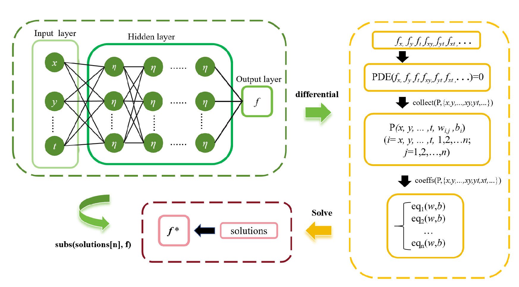
Figure 2.
Single hidden layer neural network model diagram: (a) Network structure. (b)Model[4-3-1]-1 . (c) Model[4-3-1]-2.
Figure 2.
Single hidden layer neural network model diagram: (a) Network structure. (b)Model[4-3-1]-1 . (c) Model[4-3-1]-2.
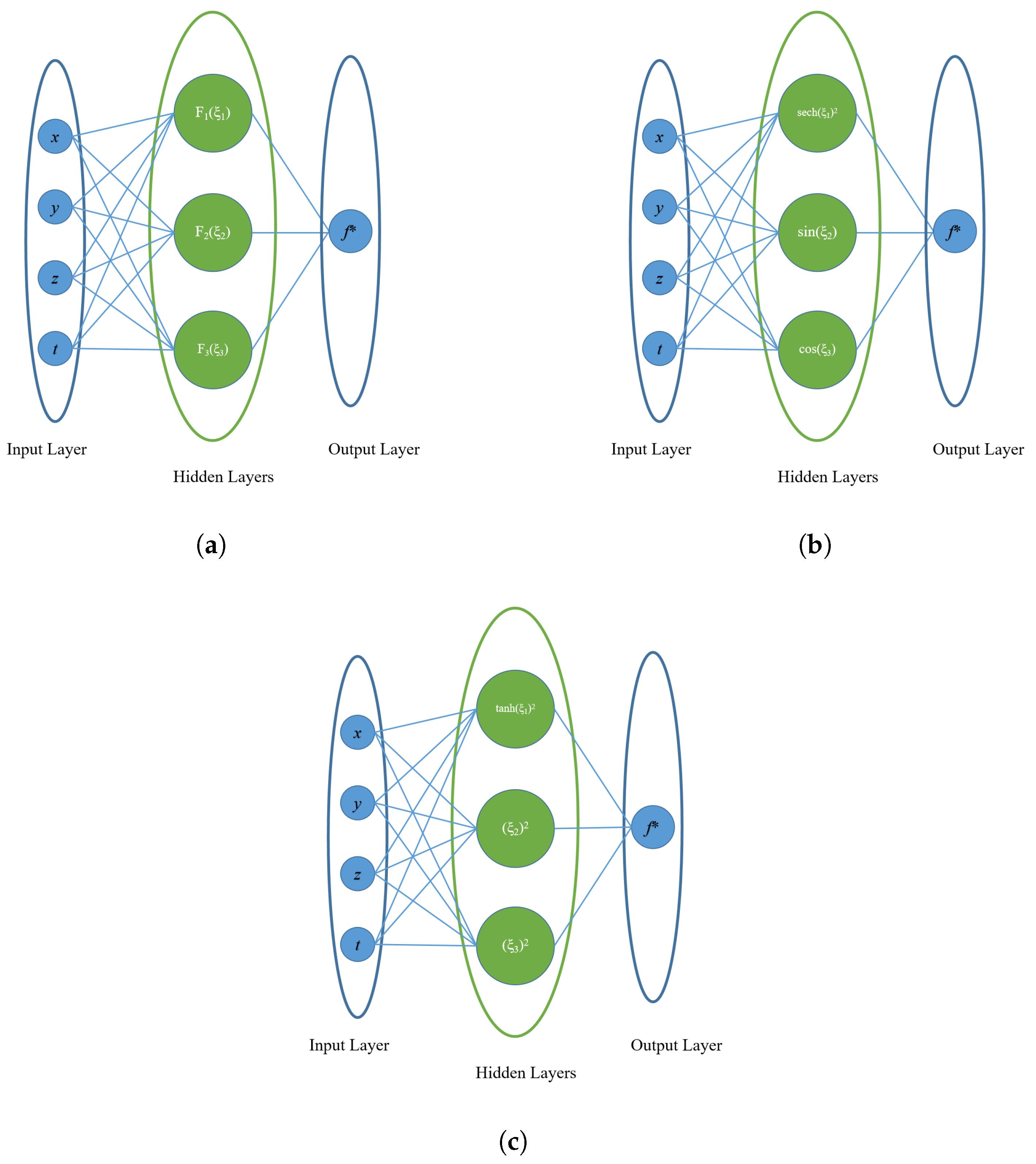
Figure 3.
Plots of the solution(5): (a) Three - dimensional graphs. (b) Contour diagrams. (c) Thermal maps. (d) Evolution plot.
Figure 3.
Plots of the solution(5): (a) Three - dimensional graphs. (b) Contour diagrams. (c) Thermal maps. (d) Evolution plot.
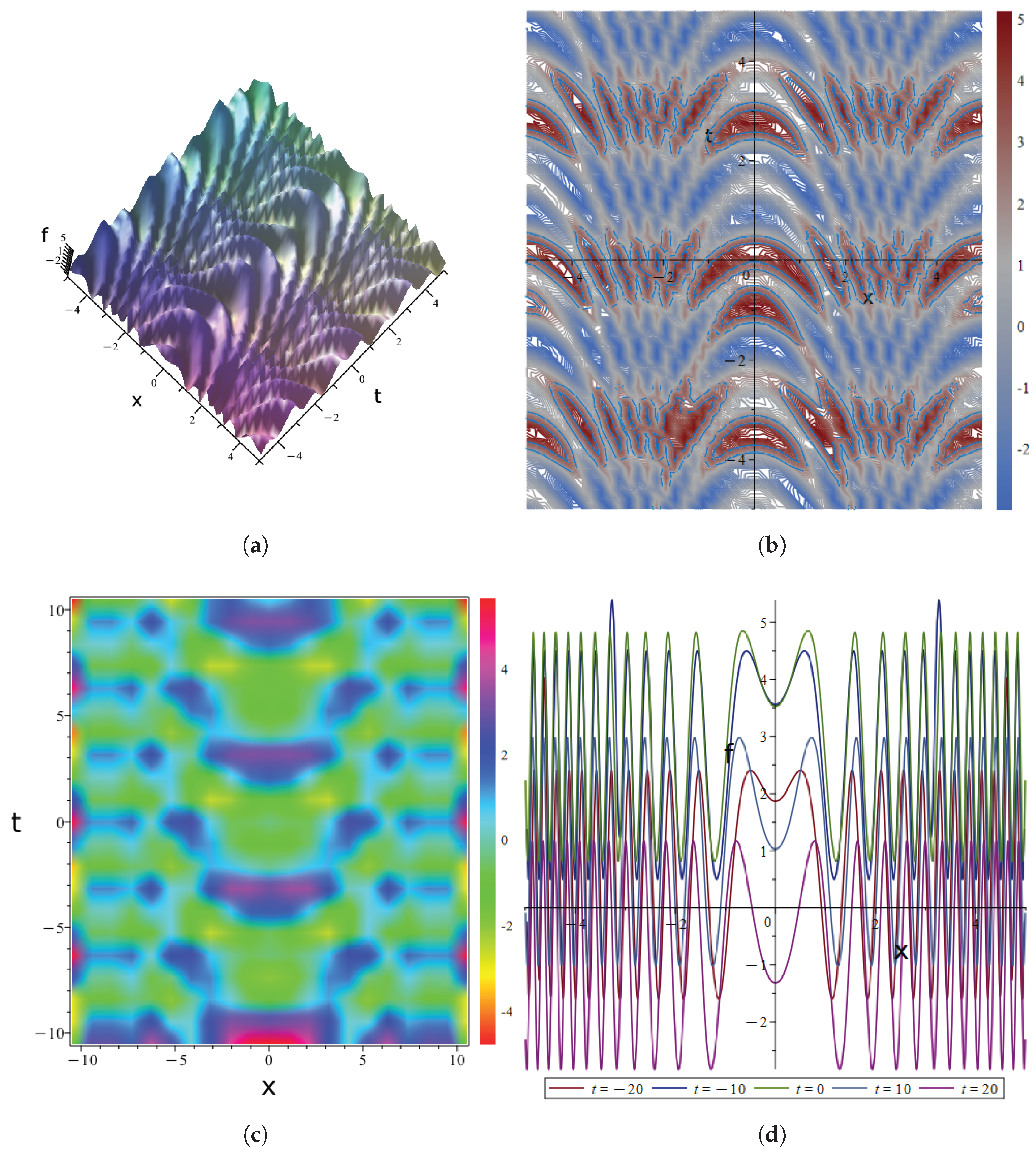
Figure 4.
Plots of the solution(6): (a) Three - dimensional graphs. (b) Contour diagrams. (c) Thermal maps. (d) Evolution plot.
Figure 4.
Plots of the solution(6): (a) Three - dimensional graphs. (b) Contour diagrams. (c) Thermal maps. (d) Evolution plot.
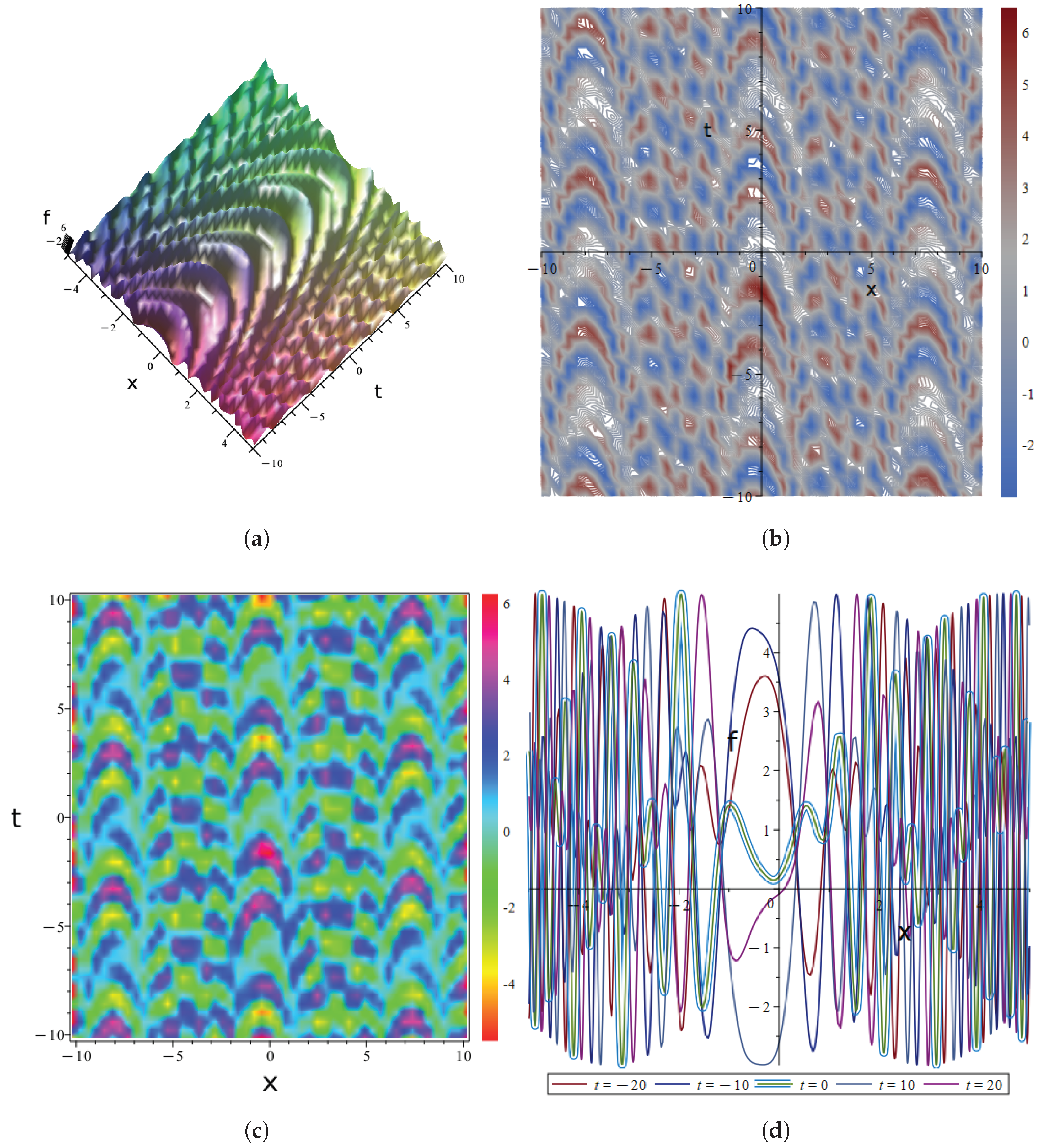
Figure 5.
Plots of the solution(10): (a) Three - dimensional graphs. (b) Contour diagrams. (c) Thermal maps. (d) Evolution plot.
Figure 5.
Plots of the solution(10): (a) Three - dimensional graphs. (b) Contour diagrams. (c) Thermal maps. (d) Evolution plot.

Figure 6.
Plots of the solution(11): (a) Three - dimensional graphs. (b) Contour diagrams. (c) Thermal maps. (d) Evolution plot.
Figure 6.
Plots of the solution(11): (a) Three - dimensional graphs. (b) Contour diagrams. (c) Thermal maps. (d) Evolution plot.
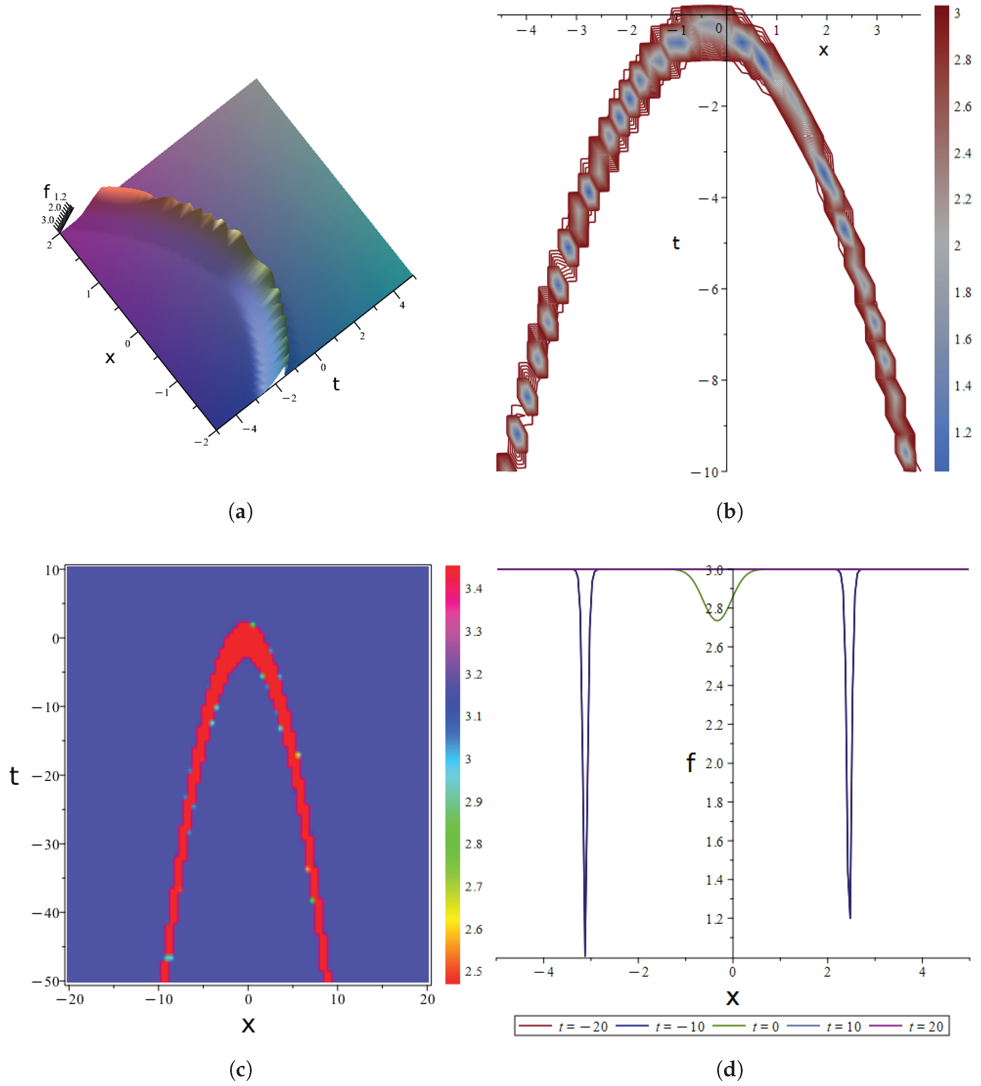
Figure 7.
Double hidden layer neural network model diagram: (a) Network structure. (b)Model[4-4-3-1]-1 .
Figure 7.
Double hidden layer neural network model diagram: (a) Network structure. (b)Model[4-4-3-1]-1 .
Figure 8.
Plots of the solution(15): (a)Three - dimensional graphs. (b) Contour diagrams. (c) Thermal maps. (d) Evolution plot.
Figure 8.
Plots of the solution(15): (a)Three - dimensional graphs. (b) Contour diagrams. (c) Thermal maps. (d) Evolution plot.
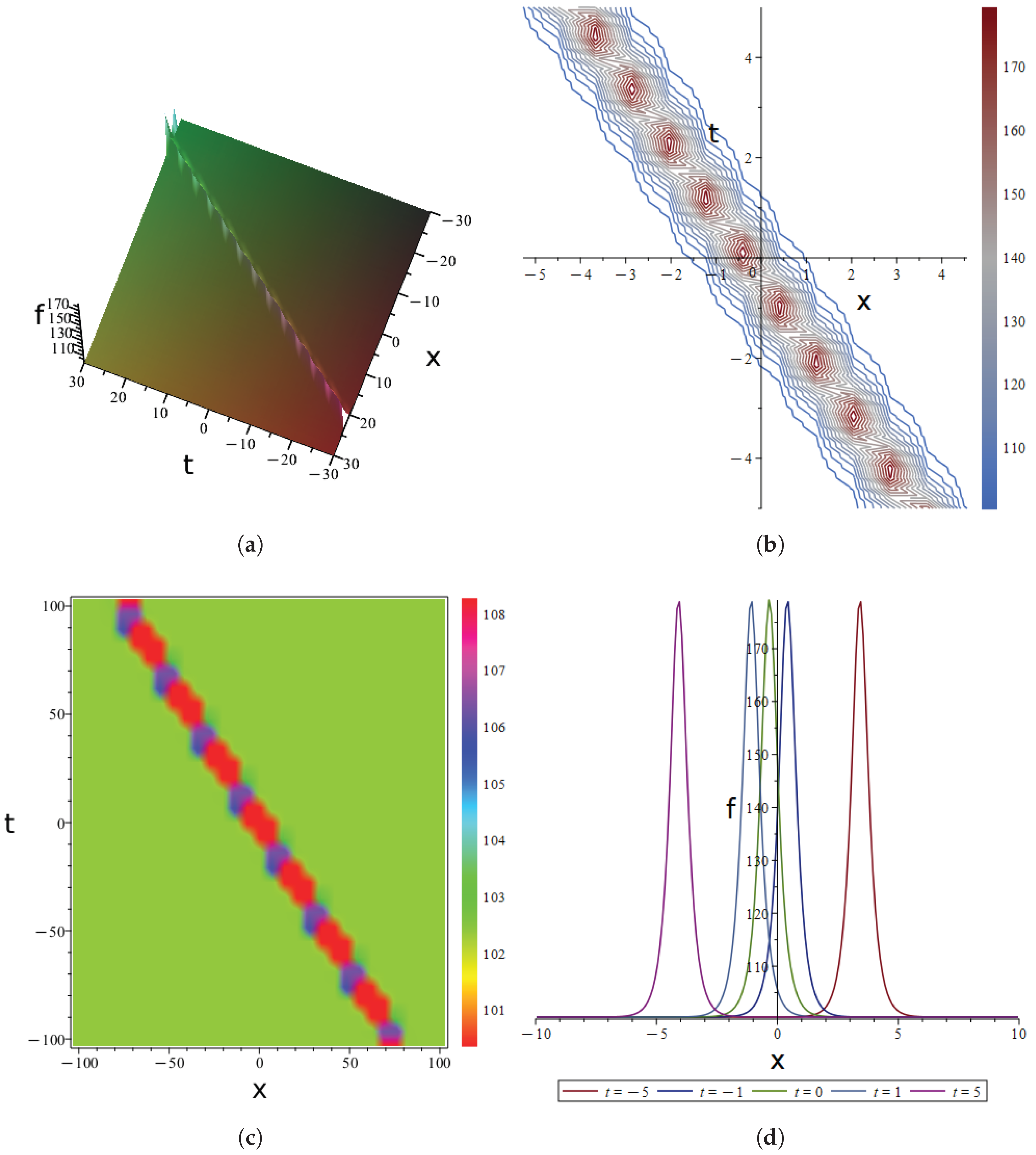
Figure 9.
Plots of the solution(16): (a) Three - dimensional graphs. (b) Contour diagrams. (c) Thermal maps. (d) Evolution plot.
Figure 9.
Plots of the solution(16): (a) Three - dimensional graphs. (b) Contour diagrams. (c) Thermal maps. (d) Evolution plot.
Disclaimer/Publisher’s Note: The statements, opinions and data contained in all publications are solely those of the individual author(s) and contributor(s) and not of MDPI and/or the editor(s). MDPI and/or the editor(s) disclaim responsibility for any injury to people or property resulting from any ideas, methods, instructions or products referred to in the content. |
© 2026 by the authors. Licensee MDPI, Basel, Switzerland. This article is an open access article distributed under the terms and conditions of the Creative Commons Attribution (CC BY) license (http://creativecommons.org/licenses/by/4.0/).
Copyright: This open access article is published under a Creative Commons CC BY 4.0 license, which permit the free download, distribution, and reuse, provided that the author and preprint are cited in any reuse.


