
Submitted:
09 January 2026
Posted:
13 January 2026
You are already at the latest version
Abstract
In ultrasonic testing, full waveform inversion (FWI) is employed to recover internal material perturbations by fitting the simulated wave fields with sparsely measured wave signals at sensor locations using gradient-based optimization. Since the underlying optimization problem is inherently ill-posed, the resulting material fields without regularization contain substantial artifacts. Neural network parameterizations have been shown to produce superior reconstructions. Incorporating prior knowledge through data-driven transfer learning can further accelerate the reconstruction. To date, such approaches have been limited to uniform grids treated using convolutional neural networks. In this work, we extend this methodology to arbitrarily shaped domains using graph convolutional networks (GCN). The GCN-based FWI exhibits strong generalization capabilities. The proposed approach for the 3D elastic wave equation can be accelerated through inexpensive pre-training on a scalar 2D dataset, resulting in faster training and more accurate reconstructions. Numerical experiments demonstrate that the proposed method can generalize well to complex 2D and 3D geometries with diverse experimental setups involving different sensor positions, sources, and material properties.
Keywords:
transfer learning
; graph convolution network
; deep learning
; adjoint optimization
; full waveform inversion
1. Introduction
Full waveform inversion (FWI) has its origins in seismic applications [10,11]. In an inversion framework, waveform information is exploited by iteratively fitting simulated data from a numerical model to measurements. In recent years, the application of FWI has also been explored in ultrasonic testing, where it can be applied for internal damage detection in solid structures thanks to its ability to reconstruct internal voids and hidden boundaries. The method involves using piezoelectric transducers to generate waves that propagate through a solid structure. These waves reflect off internal boundaries, such as cracks or other impurities, before being measured by a collection of sensors. FWI then employs an optimization process to iteratively update the material distribution of a computational model, thereby minimizing the difference between simulated and measured data. Numerical studies [12,13,14,15] and experimental validation [16] have demonstrated the enhanced tomographic capabilities of FWI compared to non-iterative approaches such as the total focusing method (TFM) [17] and reverse time migration (RTM) [18].
While classical methods using polynomial representations of material fields still dominate [11,19,20], recent studies in seismic exploration suggest that neural networks can improve the reconstruction quality by serving as efficient parameterizations for material parameter fields [21,22,23,24]. Similar benefits have been observed in structural optimization [1,2,3], where the parametrization has been coined neural topology optimization [4]. Herrmann et al. [25] extended these benefits to ultrasonic testing, demonstrating that neural network-based FWI can accurately detect internal voids. A key advantage of using neural networks as parametrizations is their ability to suppress high-frequency artifacts in the reconstructed images, thereby improving tomographic accuracy. This advantage arises because neural networks tend to learn smoother, low-frequency spatial patterns before capturing high-frequency details [26], which mitigates common artifacts in classical FWI.
However, a significant challenge remains: the performance of these neural network-based methods is highly sensitive to the initial weights of the network. To address this, researchers have proposed various advanced strategies. Vantassel et al. [27] used neural networks to generate informed initial guesses for classical FWI. Müller et al. [28] introduced a transfer learning approach that uses a network pre-trained on sensor data prior to their use in inversion. In [29], the network is pre-trained on sensor data and the corresponding damage and subsequently used for the FWI. The authors of the paper at hand further developed this idea in [30] by creating a transfer learning framework that uses adjoint gradients derived from sensor measurements to train a neural network to predict the underlying material field. This has the advantage of creating an image-to-image mapping with identical dimensions, which is agnostic to sensor and source placement. Further advances have been made by not relying on labeled data through meta-learning, in which multiple optimizations are performed with the goal of finding a better initial starting point [5].
The methods named above stand in stark contrast to purely data-driven approaches [31,32,33,34,35], which attempt to learn mappings from sensor data to material properties without incorporating physical constraints. Purely data-driven techniques cannot deliver reliable results due to the absence of an error measure on the predictions, as opposed to neural network-based optimization methods. Although such optimization methods are computationally expensive, pre-training can accelerate the minimization procedure.
A major limitation of all the aforementioned methods, whether purely data-driven or based on stringent minimization procedures constrained by the wave equation, is their reliance on grid-dependent neural network architectures, such as Convolutional Neural Networks (CNNs). These networks struggle to generalize effectively to complex, unstructured geometries that significantly deviate from their training data. This drawback impedes the application of neural network-based methods in non-academic scenarios.
To address this limitation, we propose utilizing Graph Convolutional Networks (GCNs) [36]. GCNs operate on graph-structured data (Figure 1), where nodes represent spatial points and edges encode geometric or physical relationships between them. In contrast to grid-based CNNs, GCNs inherently manage irregular topologies, which allows them to adapt to geometries starkly different from those they were trained on. This adaptability makes GCNs especially well-suited for transfer learning in Full Waveform Inversion (FWI), as they readily facilitate generalization across various geometries, especially those different from the training set.
Due to their inherent flexibility [37], GCNs have been widely adopted in domains requiring generalization over graph structures. They have been successfully applied to learning mesh-based physical simulations [6,38] and have also been integrated with Physics-Informed Neural Networks (PINNs) [39,40,41]. It is worth noting that PINNs are comparatively inefficient relative to classical methods, particularly in the context of FWI [7]. Readers seeking a comprehensive review of GCNs are directed to [42].
In this work, we propose using GCNs to parameterize the material field, an approach inspired by our prior work that utilized CNNs [25,29,30]. To the best of our knowledge, this is the first application of graph neural networks along with FWI. In particular, we demonstrate the following:
- We pre-train a GCN to learn to map an adjoint gradient, calculated from the first iteration of classical FWI, to the true material distribution. Both the input (the adjoint gradient) and the output (the material distribution) share the same underlying graph structure, enabling a simple network architecture.
- Using GCNs along with input and output data that are defined on identical graphs allows the method to be independent of specific experimental conditions, such as the number of sensors, the material’s properties, or the excitation frequency.
- Once the GCN is pre-trained, it generalizes to a wide range of setups and material characteristics (see Section 3). The network’s output then serves as the initial model for the FWI process. The GCN’s weights are subsequently fine-tuned during the FWI iterations to produce the final, refined damage distribution.
Figure 1 depicts the proposed approach.
2. Methodology
2.1. Physical Models
In the current work, we use the scalar wave equation to generate inexpensive pre-training datasets on a rectangular geometry, while, in the inversion, wave propagation is modeled using the elastic wave equation. As proposed in [12], void- or crack-like defects can be described by a degradation in the material’s density. Introducing a dimensionless scaling function , and assuming a constant density and P-wave speed of the background material, the 2D scalar wave equation in the spatial domain and for time can be written as
where is the scalar wave field, the corresponding acceleration, and f the external force. Equivalently, the 3D elastic wave equation for is given by
where the elastic wave field has three components, and the constant linear isotropic elastic constitutive tensor of undamaged material. Parametrized with the density and P- and S- wave speeds and , is written as
Additionally, homogeneous initial conditions are set at , and homogeneous Neumann boundary conditions are prescribed on .
2.2. Classical FWI
In classical FWI, the material field is commonly represented by a set of coefficients defined on the underlying computational grid or mesh. In this work, the vector contains the scaling function values at the vertices of a finite element mesh. We seek to find an optimal vector of coefficients that minimizes the misfit function :
The error is summed over all experiments and receiver positions. For the elastic wave equation, we obtain
in which represents the simulated wave field based on the coefficients , while represents the sparse measurements from the target domain (referred to as the “observed wavefield” in the subsequent text), and is a unit vector pointing in the measurement direction of the receiver. The complete set of measurements across all experiments is denoted as and is the number of receivers.
To calculate how the cost function changes with respect to material coefficients, we employ the adjoint method. For those interested in the complete mathematical derivation, see, e.g. [12]. The adjoint method allows us to compute the derivative of the misfit functional with respect to a perturbation of the density scaling function in the direction
For the elastic wave equation, the sensitivity kernel is
where is the solution of the adjoint wave equation. The gradient from all the vertex points can be directly applied in gradient-based optimization algorithms to find the optimal material coefficients. For the scalar wave equation, corresponding equations can be formulated, e.g., see [12]. In this work, the commercial software Salvus from Mondaic [43] has been used as the forward solver and for calculating the adjoint gradients.
2.3. Graph Convolutional Network-Based Transfer Learning FWI
2.3.1. Graph Convolutional Networks
GCNs are structured around the principle of message passing [8], where each node aggregates information from the nodes it is connected with to refine its representations over the layers of the network. The aggregation operations in GCNs used in the current work are based on vanilla GCNs [44], where node features are updated using weighted combinations of adjacent node attributes,
where and are the trainable parameters of the layer, is the value of the node from the previous layer, and is the value of the neighboring nodes. All the connected neighboring nodes share the same weight matrix , which is the key feature that allows the GCN to generalize to nodes with different numbers of neighbors, and thus to different graphs. Figure 2 shows the representation of a finite element mesh as a graph.
A key advantage of GCNs lies in their ability to process mesh-based data, which is inherently structured as a graph. Traditional grid-based methods struggle with irregular geometries, whereas GCNs are designed to operate on these structures. The PyTorch geometric library [45] is used, because it offers an excellent out-of-the-box implementation of many types of GCNs.
2.3.2. Pre-Training
The graph-based neural network discussed above is pre-trained using the adjoint gradients of the first iteration of a classical FWI. The same training data as used in our previous work [30], expressed as a graph, is used to pre-train the GCN. The dataset is generated by varying the semi-major and minor axes a and b, the center and , and the rotation of a single elliptical damage. The generated damaged density distributions serve as input to the wave equation to compute the corresponding wavefields . These wavefields, evaluated at the sensor locations, act as the observed wavefields . Assuming an undamaged density distribution , the adjoint gradient is calculated using the observed wavefields. These adjoint gradients form the input to the GCN. The damaged density distributions (with ellipsoidal voids) are used to generate the observed wavefield from the target output . For training the GCN, the input and the output data are converted into a graph as depicted in Figure 2. The features of the mesh nodes become the features of the nodes processed by the GCN. The GCN is trained in a supervised manner to minimize the standard mean-squared error loss function
between predicted and ground truth target values .
Neural network architecture:
The GCN has a symmetric encoder-decoder architecture designed for node-level feature transformation. The model comprises an encoder, a bottleneck layer, and a decoder, with each component constructed from a series of GCN layers, followed by Graph Normalization layer1 for feature normalization and a PReLU activation (except for the final output layer). The encoder progressively transforms the input node features through the layers, resulting in a latent embedding space. A single bottleneck layer connects the encoder and decoder. Each layer maintains the dimensionality of the output from the previous layer. The decoder reconstructs node features from the bottleneck’s output. It mirrors the encoder’s structure, with its initial layers using CuGraphSAGEConv2 with max aggregation. At the end of the decoder layer, there is a layer of SAGEConv with a Multi-Aggregation module, which combines the outputs of three parallel Softmax Aggregation modules. Each Softmax Aggregation module is parameterized by a learnable temperature , initialized to , , and respectively ( Table 4). For each module k, an aggregated feature vector is computed element-wise, where the dimension is given by
Here, denotes the feature of message . The parameter is learnable, allowing the model to adaptively fine-tune the aggregation behavior of each neighbor. Finally, three aggregated vectors are combined element-wise using the LogSumExp function of PyTorch. The final aggregated message for node v, with its dimension , is computed by
This LogSumExp combination serves as a smooth, differentiable approximation of the maximum function, enabling the GCN to dynamically emphasize the most important aggregation terms for each feature. Furthermore, the smooth nature of the function also allows better gradient flow during training as compared to other commonly used aggregation functions like max or min. The final layer of the GCN is essential since it improves the expressivity of the network. This, in turn, improves the convergence during the downstream task of TL-FWI. Adding more layers did not significantly improve the results.
Since GCNs and CNNs operate on fundamentally different data structures, there is a significant difference in their training speeds. GCNs are designed to handle irregular data structures such as graphs, where nodes can have a varying number of connections. This lack of a uniform structure means the GPU cannot apply the same highly parallel, uniform operations as it does for CNNs. Given the computational challenges, the GCN is trained on only 200 training cases as opposed to the 800 cases in our previous work [30]. This training data is based on the scalar wave equation on a rectangular 2D geometry, with a 70:30 train-test split. The corresponding training time for 200 epochs is minutes on a Nvidia Quadro RTX 8000. The input, i.e., the initial adjoint gradient, is converted into graph data using the PyTorch Geometric library. Here, the gradient value at each node of the mesh is stored as a 1D vector, and another 2D vector is constructed to represent the connectivity between all nodes. For constructing the connectivity, the radius threshold method was used. This forms the input to the GCN. The density distribution is analogously converted into a vector (in the same order as the input), which yields the output. Further details can be inferred from the code published in [46].
Pre-processing adjoint gradient:
During pre-training, the model was trained on data that is in a uniform, rectangular domain where the wavefields provided consistent illumination. This means the energy from the sources and sensors is spread evenly throughout the domain. As a result, the distortions in the gradients caused by distortions in the density due to the damage (damage fingerprint) were strong and easily detectable by the neural network. The addition of a region of interest (ROI) further refined this process by excluding near-field artifacts from the sources and sensors. In the downstream task, we tested irregular geometries and used a simulation time that was not long enough to allow the wavefields to illuminate the domain uniformly. This lack of uniform illumination caused the damage fingerprints to be weaker and difficult to detect, making them almost “invisible” to the neural network. By scaling the adjoint gradients using the wavefield, we effectively normalized the data. This resulted in the damage fingerprints being easily recognized by the neural network, resulting in better initial guesses. The scaling factor is determined as
where u is the displacement field for all node points along the x, y, and z directions, t is the time steps used for checkpointing, and i is the node. The normalized gradient is calculated by scaling the quantity
where is the adjoint gradient from the first iteration of the classical FWI. This process amplifies the weak gradients from the damaged boundaries, making them more prominent and easier for the neural network to identify. This normalization directly led to a significant improvement in the quality of the initial guesses, as the network could now reliably detect and localize the damage despite the non-uniform illumination. Figure 3 shows the gradient pre-processing steps.
Generalization to arbitrary shape and experiment configuration:
Using an adjoint gradient for pre-training the GCN instead of raw wavefields has several advantages. Most importantly, the graph network learns to map the gradient to the density scaling function on the same graph. This renders the architecture of the GCN to be independent of the number of sensors, the time steps of the raw wavefield, and the type of wave equation used (scalar or elastic) as opposed to other transfer learning approaches [28,29]. This flexible formulation constitutes a key ingredient of the paper at hand, as it enables automatic generalization to other geometries, sensor configurations, excitation locations, source types, and types of wave equations. Consequently, the data necessary to pre-train the GCN is generated cheaply, using simple rectangular geometry simulated with the scalar wave equation. The generalization capabilities are strong enough that the pre-trained GCN can be applied to FWI based on the elastic wave equation for geometrically and topologically more complex scenarios in 3D. This is remarkable, as the training data only covers a single 2D rectangular geometry on the scalar wave equation.
2.3.3. Graph Convolutional Network-Based Transfer Learning (GCN-based TL-FWI)
In transfer learning-based FWI, as proposed in [30], a CNN is used for discretization of the density scaling function . The CNN is pre-trained to identify the damage directly from the adjoint gradient calculated from the first iteration of a classical adjoint method. Using the adjoint gradient instead of the raw signal allows us to simplify the network architecture, because the input and output shapes are identical. Once trained, the network is used for the downstream task of FWI. In the paper at hand, a further step is taken towards generalization by using a GCN to parameterize the density scaling function . The developed method is termed GCN-based TL-FWI (Figure 4) in the remainder of this work. The gradients of the cost function with respect to the weights of the pre-trained GCN are calculated using the chain rule [25]. The pseudo code of the GCN-based TL-FWI algorithm is also shown in Algorithm 1.
2.4. Classical FWI with Initial Guess
Classical FWI can similarly be accelerated using the pre-trained GCNs to provide an initial guess of the damage. The initial guess serves as the starting model for a classical FWI method, where the material field is defined by a set of coefficients defined on the underlying computational grid or mesh. In this work, the L-BFGS optimization method from the PyTorch library was used to solve the optimization task. The pseudo code for classical FWI algorithm is shown in 2. Comparing the GCN-based TL-FWI with a classical FWI (provided with the same initial guess) isolates the regularizing effect of the GCN on the FWI.
3. Results
3.1. Bridge to Previous Work
In order to set a point of reference of established work, the performance of a pre-trained GCN is compared to that of a CNN from [30], where a scalar wave equation has been used for carrying out FWI.
Figure 5 shows that the CNN provides a better initial guess as compared to the GCN. Additionally, the CNN recovers all voids with higher accuracy and slightly faster in the inversion than the GCN. Both the CNN-based and GCN-based TL-FWI require fewer than 15 epochs to reconstruct the damage shapes. The reconstruction of the CNN-based TL-FWI contains fewer artifacts in the undamaged domain, and the resolved damage shape is very sharp. GCN-based TL-FWI requires some additional epochs to achieve the same level of accuracy. There are various reasons for the better performance of a CNN as compared to a GNN. Section 4 contains a detailed discussion about the differences between a CNN and a GCN. The drawbacks of GCN are largely offset by its generalization capabilities, as will be demonstrated in the sequel.
Note that the double voids depicted in Figure 5 were also outside the training dataset; the present case depicts the performance of the GCN on an arbitrary damage scenario. While CNN-based FWI may achieve faster convergence in the simple rectangular scenario, GCNs offer greater flexibility for handling more complex and unstructured geometries, which is crucial in cases where the investigated domain deviates significantly from a simple rectangle.
3.2. Generalization to 2D T-Shaped Geometry and Elastic Wave Equation
The generalization capability of the GCN-based TL-FWI is presented step by step, starting from the simplest case of a T-shaped 2D geometry, which presents a moderate generalization challenge. As previously elaborated, GCNs allow generalizing to arbitrary meshes by converting the mesh (and the corresponding quantities defined on the mesh nodes) into a graph. The details can be found in Section 2.3.2. The performance of GCN-based TL-FWI is compared with classical FWI with and without an initial guess from the pre-trained GCN (as described in Section 2.4).
3.2.1. Experimental Configuration
Moving from the initial rectangular 2D training domain (which relied on the scalar wave equation), first, we assess the generalization to a T-shaped domain and to the elastic wave equation. Furthermore, different material properties and excitation frequencies are utilized. The T-shaped geometry and the corresponding mesh were generated using the Gmsh library in Python. It was then converted into Exodus format using the Pyexodus library and read into the Salvus [47] solver from the software framework published by Mondaic AG in Python. The pre-trained GCN outputs the density values at the corresponding vertices of the mesh. For the simulation of elastic wave propagation, point sources were utilized. Unlike the scalar case, which typically involves a single force component or pressure source, the elastic simulations utilize vector point sources capable of generating both horizontal and vertical force components. The source time function for these simulations is a Ricker wavelet. The details of the simulation and the material properties are provided in Table 1.
The initial guess is also used as the starting model for the classical FWI. L-BFGS was used for the optimization of the classical method, whereas Adam [9] is utilized for the GCN-based TL-FWI. As the L-BFGS optimizer relies on multiple function evaluations per epoch, a comparison based on the number of epochs is unfair. Instead, the results are compared at specific times. Overall, the 10 iterations of L-BFGS optimization are approximately equivalent to the 75 iterations of Adam in terms of runtime.
3.2.2. Results
Good initial guess:
The GCN-based TL-FWI is used for detecting a simple scenario consisting of a single damage. The initial guess in Figure 6 (a) shows that the network is able to correctly guess the location of the damage. As a reference, classical FWI with the initial guess is also used to detect the same damage. The convergence results are shown in Figure 6. It shows that the TL-FWI method is much faster than the classical methods. At , the TL-FWI method has already recovered the complete damage shape with negligible artifacts, while the classical FWI is unable to recover the shape accurately, even after .3. This highlights the capability of the proposed GCN-based TL-FWI method in reconstructing the damage shape accurately and faster than the classical FWI method.
Bad initial guess:
The following case contains three voids presenting a greater challenge. The pre-trained GCN only predicts a small portion of the damage closest to the sensors (and is unable to predict the other two), see Figure 7 (b). Furthermore, incorrect voids are predicted in the bottom left corner.
During the optimization cycles of FWI, the GCN-based TL-FWI is able to correct the bad initial guess, see Figure 7 (c). The mean squared error of the final reconstruction is . The classical FWI with the initial guess (Figure 7 (d)) is also able to recover the voids. However, the recovered shapes are not as accurate (mean squared error ). Furthermore, the classical FWI required as compared to GCN-based TLFWI, which required . In particular, this demonstrates that classical FWI suffers from substantial noise even if the same prediction is given as a starting point for the iteration, as in the case of the GCN, as well as requiring more time. Therefore, it can be concluded that GCN-based TL-FWI still works the best at reconstructing damage on a T-shaped geometry despite a bad initial guess.
3.3. Generalization to 3D Geometry: Flange
The next numerical example demonstrates the ability of the GCN-based TL-FWI to generalize to a 3D flange geometry, which is a common mechanical component. The focus is on the prediction of the pre-trained GCN, which has only been trained on 2D rectangular domains.

Table 2.
Properties of the simulation for Flange
| Property | Value |
|---|---|
| Excitation frequency | |
| Simulation time | s |
3.3.1. Numerical Configuration
The flange, with an outer radius of m and an inner radius of m, has a thickness of m. As shown in Figure 8(a), it contains five known holes and two ellipsoidal internal damages located near them. For data acquisition, five sensors and 25 receivers are positioned on the outer radius and at half the thickness of the flange. The GCN, which is pre-trained on a 2D rectangle (Figure 1), is now applied to a Flange’s complex geometry. Figure 8(b) shows the initial gradient, which is the input to the pre-trained GCN. The initial gradient was pre-processed in the same way as described in the previous section (Section 2.3.2.2).
3.3.2. Results
Figure 8(a) shows two damaged areas located near holes in a flange. The initial prediction provided by our GCN, shown in Figure 8(b), accurately predicts the location of these damaged regions. However, it also incorrectly identifies a damaged area at the bottom of the flange. This false positive is likely due to strong reflections from the hole boundaries, which can produce high gradients that the GCN interprets as damage.
Classical FWI successfully recovers both damaged areas, but with significant artifacts, particularly in the vicinity of the damage(Figure 8(d)). The recovered shapes are generally satisfactory, but the widespread artifacts are a common issue with classical FWI (mean-squared error ). The runtime of classical FWI was approximately 13.7 hours. The proposed GCN-based TL-FWI (Figure 8(c)) outperforms the classical method as it recovers the damaged areas with higher accuracy (mean-squared error ) and substantially less noise in about half the time (5.5 hours).
3.4. Generalization to 3D Geometry: Cylinderical Column
This numerical example demonstrates the ability of the GCN-based TL-FWI to generalize to another 3D geometry of a support column, a geometry that is quite common in civil engineering.
3.4.1. Numerical Configuration
The column has a radius of m in the center, a radius of m at the base, and a length of m (Figure 9). There are four sources and 32 receivers placed on the outer surface of the column at a height of m and m from the base. A significant challenge is presented by the stark difference in numerical configurations; the new geometry is considerably larger, and the excitation frequency is two orders of magnitude lower. The GCN, which is pre-trained on the 2D rectangle as shown in Figure 1 with much higher excitation frequency, is now applied to the column for reconstructing the scaling function (Figure 9(a)). The initial gradient was preprocessed in the same way as described in Section 2.3.2.2 before being input to the pre-trained GCN.
Table 3.
Properties of the simulation for cylindrical column
| Property | Value |
|---|---|
| Excitation frequency | |
| Simulation time | |
| Density | |
3.4.2. Results
Despite the substantial differences in the configuration of the pre-training, the GCN successfully predicts the correct location of the damage (Figure 9(b)) in the computation. While the initial prediction of the damage shape was found to be imperfect, its accurate localization is still very beneficial in accelerating the GCN-based TL-FWI. This preliminary damage estimate is then used as a starting model for the subsequent GCN-based TL-FWI process.
The final reconstructed scaling function obtained via GCN-based TL-FWI in (Figure 9(c)) and classical FWI with an initial guess is shown in (Figure 9(d)). The GCN-based TL-FWI method results in the most accurate scaling function reconstruction, closely matching the actual shape of the defect. The favorable difference in terms of noise becomes evident in the final reconstruction when comparing to the results obtained by classical FWI (Figure 9(d)). Although the computational time for both methods is comparable in this case, the mean-squared error (MSE) for GCN-based TL-FWI is , which is significantly lower than the recorded for classical FWI with the initial guess. This difference demonstrates the GCN-based TL-FWI’s capability to generalize well and effectively suppress artifacts, even within complex 3D geometries.
4. Discussion
The proposed GCN-based TL-FWI is able to accurately predict the damage even in 3D cases after being trained on data generated from the 2D rectangle depicted in Figure 1. The GCN-based TL-FWI possesses a much stronger generalization in terms of geometry, material properties, sensor placement, and excitation frequencies as compared to a CNN as used in [30]. Even in cases when the adjoint gradient from the first iteration does not contain information to allow the GCN to provide a good initial guess, the pretrained GCN is still able to recover the damage much faster than classical FWI, given the identical initial guess.
However, in comparison to the U-net [30], GCNs are more difficult and slower to train, but offer much better generalization properties. The difference in the performance between CNNs and GCNs is attributed to their fundamentally distinct architectural designs. Structured, grid-based data is processed by CNNs through the application of fixed-size convolutional kernels. The weights in a CNN are specific to each position, enabling the detection of spatially localized patterns. While this approach is effective for uniform grids, such as those found in images, its adaptability to irregular or varying geometries is limited, as the learned weights are inherently tied to the spatial arrangement of the training data.
By contrast, a graph-based representation is processed by GCNs, wherein spatial points are represented as nodes and their connectivity is encoded as edges. For each new geometry, a graph must be constructed to reflect the specific topological relationships. This fundamentally differentiates GCNs from CNNs. This graph construction introduces a minor additional overhead, as the node-edge relationships suitable for each geometry must be defined.
Information from neighboring nodes is aggregated in GCNs using a shared, trainable weight, with the receptive field determined by the graph’s connectivity and number of layers. This adaptability is critical in TL-FWI, where the density field is parameterized by the GCN, and damage distributions are predicted across structures of various scales and experimental configurations.
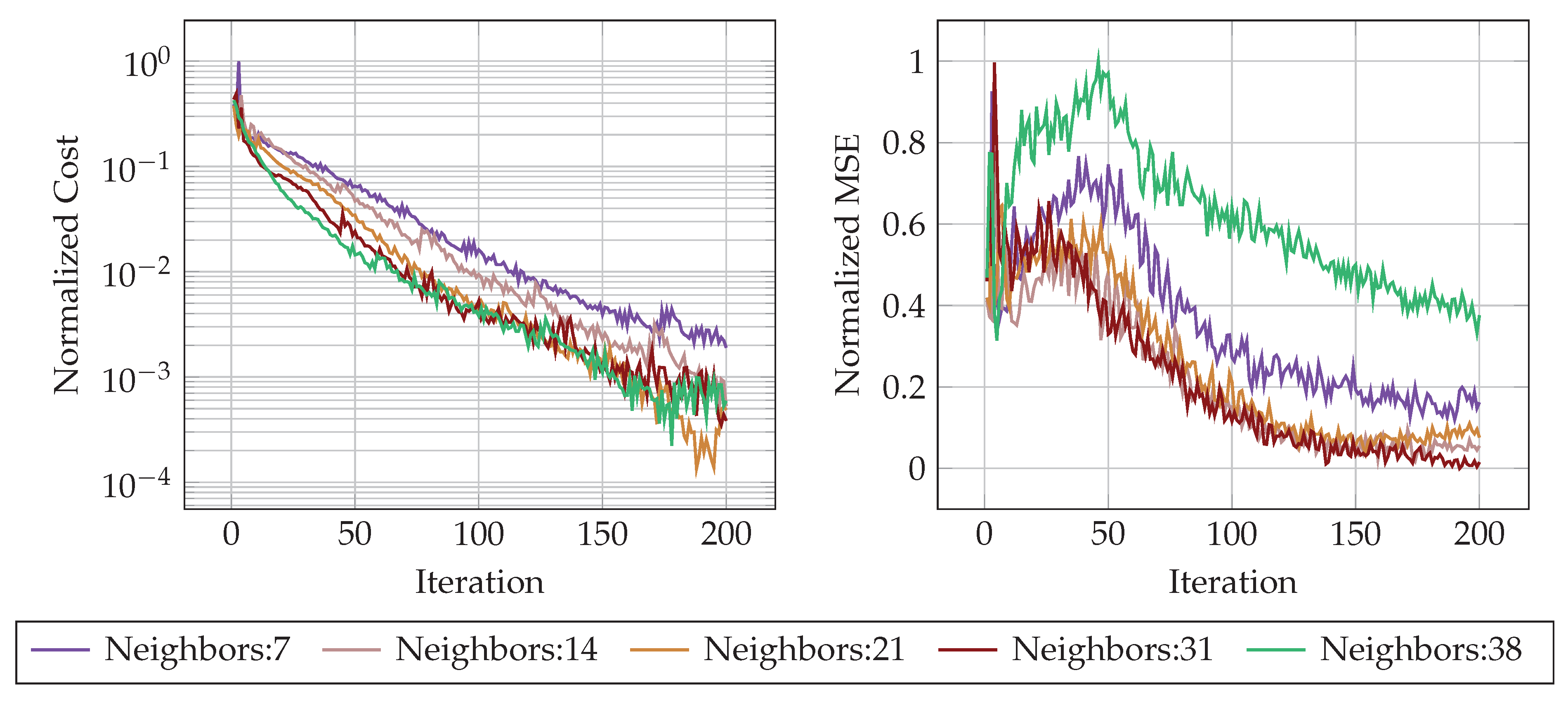
Influence of the number of neighbors:
The number of neighboring nodes considered in a GCN’s aggregation process is a pivotal hyperparameter that governs the trade-off between reconstruction accuracy and computational feasibility. A larger number of neighbors expands the receptive field, providing richer contextual information that helps in noise suppression and improves the accuracy of the damage reconstruction using TL-FWI. As illustrated in Figure 10, increasing the number of neighbors accelerates convergence of FWI and reduces the mean squared error (MSE) by capturing wider spatial dependencies. However, this benefit is also accompanied by the risk of oversmoothing, where excessive neighbor aggregation dilutes fine-scale damage features by incorporating irrelevant information from distant nodes.
Limitations of GCN-based TL-FWI:
Memory constraints further complicate the trade-off between the number of neighbors and TL-FWI convergence. The memory cost of GCNs scales linearly with respect to the number of nodes and the number of neighbors, as each node’s feature update requires aggregating high-dimensional representations. Therefore, selecting an optimal number of neighbors presents a trade-off between achieving the desired predictive accuracy and speed, and satisfying the computational and memory requirements of the system. Graph connectivity is a hyperparameter that can be adjusted based on available computational resources without altering the network architecture. This is a key consideration that sets GCNs apart from CNNs. Furthermore, the memory requirement also increases with the number of nodes in the finite element mesh. In the presented case studies, the peak memory requirement reached the maximum capacity of the GPU (48 GB) for the flange, which had roughly nodes. In other words, the increase in the speed that is possible due to GCN-based TL-FWI comes at the cost of increased peak memory usage.
However, various methods have already been proposed to tackle the high memory requirements of big GCNs, such as using mixed precision, where the forward and backward pass of the neural network is carried out in half precision instead of full precision, which halves the memory requirement. Another method exploits subgraph sub-sampling [48,49,50] where instead of training the whole graph, small graphs are sampled from the large graph and trained in mini-batches. Gradient checkpointing [51] can be used as well. Instead of storing all intermediate activations of the network, only a selected few are saved, and during backpropagation, the unsaved activations are recomputed on-the-fly. All these recent developments promise a reduction of the high memory requirement of GCN-based TL-FWI.
5. Conclusions
This paper improves the Transfer-Learning Full Wave Form Inversion (TL-FWI) method proposed in [30] by replacing the CNN with a GCN. The advantage of using a GCN is its ability to generalize to any geometry. Additionally, pre-training is applied [30] where the adjoint gradient computed from the first iteration of classical FWI is used as an input to train the GCN to guess the corresponding damage density distribution . Using pre-training along with a GCN enables the presented method to be agnostic to geometry, experimental configuration (such as excitation frequency and number of sensors), material properties, and even specific wave physics. As demonstrated by various numerical case studies, the proposed method enables training the GCN on data generated from a 2D rectangle, as depicted in Figure 1, using the scalar wave equation. The pre-trained network is then able to generalize to 3D geometries of entirely different scales, with varying experimental configurations, different material properties, and applied to the elastic wave equation instead of the scalar wave equation. This is of great advantage, since using CNNs, as in [30], requires rectangular domains and application-specific pre-training, which is too costly in engineering-relevant scenarios.
The proposed GCN-based TL-FWI provides a good initial guess based on the adjoint gradient. Furthermore, GCN-based TL-FWI is able to reconstruct the damage faster than classical FWI and, at the same time, exhibits fewer artifacts.
The primary drawback of the proposed method is its high memory requirements. For future work, new methods will be explored to optimize the GCN so that larger geometries can be tackled and data from real-world experiments may be applied.
GCN Architecture
The GCN has an encoder-decoder architecture. The graph nodes are kept the same, and the number of channels is increased from one 256 till the bottleneck layer and subsequently reduced back to one in the final layer. The encoder part of the network is frozen. It was observed that unfreezing the weights did not improve the overall performance.
Table 4.
Graph convolutional NN architecture has an encoder-decoder type architecture. The network consists of an encoder layer, a bottleneck layer, and a decoder layer. The total number of parameters is . However, the encoder layer’s weights are frozen, which results in 351180 trainable parameters.
| Layer | Shape after layer | Learnable parameters |
|---|---|---|
| Input | 0 | |
| Encoder layer | ||
| Graph Convolution with Max Aggr & GN & PReLU | ||
| Graph Convolution with Max Aggr & GN & PReLU | ||
| Graph Convolution with Max Aggr & GN & PReLU | ||
| Graph Convolution with Max Aggr & GN & PReLU | ||
| Graph Convolution with Max Aggr & GN & PReLU | ||
| Bottleneck layer | ||
| Graph Convolution with Max Aggr & GN & PReLU | ||
| Decoder layer | ||
| Graph Convolution with Max Aggr & GN & PReLU | ||
| Graph Convolution with Max Aggr & GN & PReLU | ||
| Graph Convolution with Max Aggr & GN & PReLU | ||
| Graph Convolution with Max Aggr & GN & PReLU | ||
| Graph Convolution with Multi Aggr & GN & Sigmoid |
GCN-Based TLFWI Pseudocode
| Algorithm 1: GCN-based Transfer Learning FWI |
|
Classical FWI with Initial Guess
| Algorithm 2: Classical FWI with initial guess FWI |
|
Data Availability Statement
We provide an implementation using Pytorch and Salvus for all methods in [46].
Acknowledgments
The authors gratefully acknowledge the funding provided by the Georg Nemetschek Institut (GNI) through the joint research project DeepMonitor, which finances Divya Shyam Singh. Furthermore, we gratefully acknowledge funds received by the Deutsche Forschungsgemeinschaft under Project no. 438252876, Grant KO 4570/1-2 and RA 624/29-2 which supports Tim Bürchner and Leon Herrmann. Lastly, we want to thank Mondaic AG for providing Salvus licenses which were used to efficiently compute the forward problem of wave propagation.
Conflicts of Interest
No potential conflict of interest was reported by the authors.
References
- Hoyer, S.; Sohl-Dickstein, J.; Greydanus, S. Neural reparameterization improves structural optimization. arXiv 2019, arXiv:1909.04240. [Google Scholar] [CrossRef]
- Chandrasekhar, A.; Suresh, K. TOuNN: Topology Optimization using Neural Networks. Structural and Multidisciplinary Optimization 2021, 63, 1135–1149. [Google Scholar] [CrossRef]
- Herrmann, L.; Sigmund, O.; Li, V.M.; Vogl, C.; Kollmannsberger, S. On neural networks for generating better local optima in topology optimization. Structural and Multidisciplinary Optimization 2024, 67, 192. [Google Scholar] [CrossRef]
- Sanu, S.M.; Aragon, A.M.; Bessa, M.A. Neural topology optimization: the good, the bad, and the ugly. arXiv 2024, arXiv:2407.13954. [Google Scholar] [CrossRef]
- Kuszczak, I.; Kus, G.; Bosi, F.; Bessa, M.A. Meta-neural Topology Optimization: Knowledge Infusion with Meta-learning. arXiv 2025, arXiv:2502.01830. [Google Scholar] [CrossRef]
- Sanchez-Gonzalez, A.; Godwin, J.; Pfaff, T.; Ying, R.; Leskovec, J.; Battaglia, P.W. Learning to Simulate Complex Physics with Graph Networks. arXiv 2020, 2002.09405. [Google Scholar] [CrossRef]
- Herrmann, L.; Kollmannsberger, S. Deep learning in computational mechanics: a review. Computational Mechanics 2024, 74, 281–331. [Google Scholar] [CrossRef]
- Battaglia, P.W.; Hamrick, J.B.; Bapst, V.; Sanchez-Gonzalez, A.; Zambaldi, V.; Malinowski, M.; Tacchetti, A.; Raposo, D.; Santoro, A.; Faulkner, R.; et al. Relational inductive biases, deep learning, and graph networks. arXiv 2018, arXiv:1806.01261. [Google Scholar] [CrossRef]
- Kingma, D.P.; Ba, J. Adam: A Method for Stochastic Optimization. arXiv 2017, arXiv:1412.6980. [Google Scholar] [CrossRef]
- Tarantola, A. Inversion of seismic reflection data in the acoustic approximation. GEOPHYSICS 1984, 49, 1259–1266. [Google Scholar] [CrossRef]
- Fichtner, A. Full Seismic Waveform Modelling and Inversion 2011.
- Bürchner, T.; Kopp, P.; Kollmannsberger, S.; Rank, E. Immersed boundary parametrizations for full waveform inversion. Computer Methods in Applied Mechanics and Engineering 2023, 406, 115893. [Google Scholar] [CrossRef]
- Bürchner, T.; Kopp, P.; Kollmannsberger, S.; Rank, E. Isogeometric multi-resolution full waveform inversion based on the finite cell method. Computer Methods in Applied Mechanics and Engineering 2023, 417, 116286. [Google Scholar] [CrossRef]
- Wen, J.; Jiang, C.; Chen, H. Detection of Multi-Layered Bond Delamination Defects Based on Full Waveform Inversion; Sensors: Basel, Switzerland, 2024; Volume 24. [Google Scholar]
- Reichert, I.; Lahmer, T. Wave-based fault detection in concrete by the Full Waveform Inversion considering noise. Procedia Structural Integrity, 2024. [Google Scholar]
- Bürchner, T.; Schmid, S.; Bergbreiter, L.; Rank, E.; Kollmannsberger, S.; Grosse, C.U. Quantitative comparison of the total focusing method, reverse time migration, and full waveform inversion for ultrasonic imaging. Ultrasonics 2025, 155, 107705. [Google Scholar] [CrossRef]
- Holmes, C.; Drinkwater, B.W.; Wilcox, P.D. Post-processing of the full matrix of ultrasonic transmit–receive array data for non-destructive evaluation. NDT & E International 2005, 38, 701–711. [Google Scholar] [CrossRef]
- Baysal, E.; Kosloff, D.D.; Sherwood, J.W.C. Reverse time migration. GEOPHYSICS 1983, 48, 1514–1524. [Google Scholar] [CrossRef]
- Böhm, C.; Martiartu, N.K.; Vinard, N.; Balic, I.J.; Fichtner, A. Time-domain spectral-element ultrasound waveform tomography using a stochastic quasi-Newton method. In Proceedings of the Medical Imaging, 2018. [Google Scholar]
- Trinh, P.T.; Brossier, R.; Métivier, L.; Tavard, L.; Virieux, J. Efficient time-domain 3D elastic and viscoelastic full-waveform inversion using a spectral-element method on flexible Cartesian-based mesh. GEOPHYSICS 2019. [Google Scholar] [CrossRef]
- Wu, Y.; McMechan, G.A. Parametric convolutional neural network-domain full-waveform inversion. GEOPHYSICS 2019, 84, R881–R896. [Google Scholar] [CrossRef]
- He, Q.; Wang, Y. Reparameterized full-waveform inversion using deep neural networks. GEOPHYSICS 2021, 86, V1–V13. [Google Scholar] [CrossRef]
- Zhu, W.; Xu, K.; Darve, E.; Biondi, B.; Beroza, G.C. Integrating deep neural networks with full-waveform inversion: Reparameterization, regularization, and uncertainty quantification. GEOPHYSICS 2021, 87, R93–R109. [Google Scholar] [CrossRef]
- Guo, K.; Zong, Z.; Yang, J.; Tan, Y. Parametric elastic full waveform inversion with convolutional neural network. Acta Geophysica 2023, 72, 673–687. [Google Scholar] [CrossRef]
- Herrmann, L.; Bürchner, T.; Dietrich, F.; Kollmannsberger, S. On the use of neural networks for full waveform inversion. Computer Methods in Applied Mechanics and Engineering 2023, 415, 116278. [Google Scholar] [CrossRef]
- Rahaman, N.; Baratin, A.; Arpit, D.; Draxler, F.; Lin, M.; Hamprecht, F.; Bengio, Y.; Courville, A. On the Spectral Bias of Neural Networks. In Proceedings of the Proceedings of the 36th International Conference on Machine Learning. PMLR, 2019; pp. 5301–5310. [Google Scholar]
- Vantassel, J.P.; Kumar, K.; Cox, B.R. Using convolutional neural networks to develop starting models for near-surface 2-D full waveform inversion. Geophysical Journal International 2022, 231, 72–90. [Google Scholar] [CrossRef]
- Muller, A.P.O.; Costa, J.C.; Bom, C.R.; Klatt, M.; Faria, E.L.; de Albuquerque, M.P.; de Albuquerque, M.P. Deep pre-trained FWI: where supervised learning meets the physics-informed neural networks. Geophysical Journal International 2023, 235, 119–134. [Google Scholar] [CrossRef]
- Kollmannsberger, S.; Singh, D.; Herrmann, L. Transfer Learning Enhanced Full Waveform Inversion*. In Proceedings of the 2023 IEEE/ASME International Conference on Advanced Intelligent Mechatronics (AIM), 2023; IEEE; pp. 866–871. [Google Scholar] [CrossRef]
- Singh, D.S.; Herrmann, L.; Sun, Q.; Bürchner, T.; Dietrich, F.; Kollmannsberger, S. Accelerating full waveform inversion by transfer learning. In Computational Mechanics; 2025. [Google Scholar] [CrossRef]
- Yang, F.; Ma, J. Deep-learning inversion: A next-generation seismic velocity model building method. GEOPHYSICS 2019, 84, R583–R599. [Google Scholar] [CrossRef]
- Wu, Y.; Lin, Y. InversionNet: An Efficient and Accurate Data-Driven Full Waveform Inversion. IEEE Transactions on Computational Imaging 2020, 6, 419–433. [Google Scholar] [CrossRef]
- Wang, W.; Ma, J. Velocity model building in a crosswell acquisition geometry with image-trained artificial neural networks. GEOPHYSICS 2020, 85, U31–U46. [Google Scholar] [CrossRef]
- Rao, J.; Yang, F.; Mo, H.; Kollmannsberger, S.; Rank, E. Quantitative reconstruction of defects in multi-layered bonded composites using fully convolutional network-based ultrasonic inversion. Journal of Sound and Vibration 2023, 542, 117418. [Google Scholar] [CrossRef]
- Kleman, C.; Anwar, S.; Liu, Z.; Gong, J.; Zhu, X.; Yunker, A.; Kettimuthu, R.; He, J. Full Waveform Inversion-Based Ultrasound Computed Tomography Acceleration Using Two-Dimensional Convolutional Neural Networks. Journal of Nondestructive Evaluation, Diagnostics and Prognostics of Engineering Systems 2023, 6. [Google Scholar] [CrossRef]
- Scarselli, F.; Gori, M.; Tsoi, A.C.; Hagenbuchner, M.; Monfardini, G. The Graph Neural Network Model. IEEE Transactions on Neural Networks 2009, 20, 61–80. [Google Scholar] [CrossRef]
- Xu, K.; Hu, W.; Leskovec, J.; Jegelka, S. How Powerful are Graph Neural Networks? 2018. [Google Scholar] [CrossRef]
- Pfaff, T.; Fortunato, M.; Sanchez-Gonzalez, A.; Battaglia, P.W. Learning Mesh-Based Simulation with Graph Networks. 2020. [Google Scholar] [CrossRef]
- Gao, H.; Zahr, M.J.; Wang, J.X. Physics-informed graph neural Galerkin networks: A unified framework for solving PDE-governed forward and inverse problems. Computer Methods in Applied Mechanics and Engineering 2022, 390, 114502. [Google Scholar] [CrossRef]
- Taghizadeh, M.; Nabian, M.A.; Alemazkoor, N. Multifidelity graph neural networks for efficient and accurate mesh-based partial differential equations surrogate modeling. In Computer-Aided Civil and Infrastructure Engineering; 2024. [Google Scholar] [CrossRef]
- Shukla, K.; Xu, M.; Trask, N.; Karniadakis, G.E. Scalable algorithms for physics-informed neural and graph networks. Data-Centric Engineering 2022, 3. [Google Scholar] [CrossRef]
- Zhou, J.; Cui, G.; Hu, S.; Zhang, Z.; Yang, C.; Liu, Z.; Wang, L.; Li, C.; Sun, M. Graph neural networks: A review of methods and applications. AI Open 2020, 1, 57–81. [Google Scholar] [CrossRef]
- Afanasiev, M.; Boehm, C.; van Driel, M.; Krischer, L.; Rietmann, M.; May, D.A.; Knepley, M.G.; Fichtner, A. Modular and flexible spectral-element waveform modelling in two and three dimensions. Geophysical Journal International 2019, 216, 1675–1692. [Google Scholar] [CrossRef]
- Bresson, X.; Laurent, T. Residual Gated Graph ConvNets. 2017. [Google Scholar] [CrossRef]
- Fey, M.; Lenssen, J.E. Fast Graph Representation Learning with PyTorch Geometric. 2019. [Google Scholar] [CrossRef]
- Singh, D.S.; Herrmann, L.; Bürchner, T.; Dietrich, F.; Kollmannsberger, S. Graph Neural Networks for full waveform inversion. 2025. [Google Scholar]
- mondaic, I. Salvus solver from mondaic, 2025. 29 05 2025. Available online: https://www.mondaic.com.
- Shi, Z.; Liang, X.; Wang, J. LMC: Fast Training of GNNs via Subgraph Sampling with Provable Convergence. ArXiv 2023. [Google Scholar]
- Shu, D.W.; Kim, Y.J.; Kwon, J. Localized curvature-based combinatorial subgraph sampling for large-scale graphs. Pattern Recognit. 2023, 139, 109475. [Google Scholar] [CrossRef]
- Zhang, Q.; Sun, Y.; Hu, Y.; Wang, S.; Yin, B. A subgraph sampling method for training large-scale graph convolutional network. Inf. Sci. 2023, 649, 119661. [Google Scholar] [CrossRef]
- Chen, T.; Xu, B.; Zhang, C.; Guestrin, C. Training Deep Nets with Sublinear Memory Cost. ArXiv 2016. [Google Scholar]
| 1 | GraphNorm is a normalization technique used in graph neural networks (GCNs) to normalize node features across graphs. It is similar to BatchNorm but tailored for graph data. |
| 2 |
CuGraphSAGEConv is a Pytorch function that implements the GraphSAGE convolution operation using cuGraph-ops on GPUs for high performance. |
| 3 | Only the classical FWI with initial guess is shown, as it is the superior classical method |
Figure 1.
Flowchart illustrating the proposed GCN-based transfer learning FWI. By using a GCN for a transfer learning-based full waveform inversion, it is possible to pre-train on a 2D rectangle under different damage scenarios and perform predictions for 3D geometries with different material properties, different numbers of sensors, source locations, and excitation frequencies. This makes pre-training extremely inexpensive, which can be performed on easy-to-generate 2D data. The pre-training accelerates the TL-FWI through the transfer of prior knowledge.
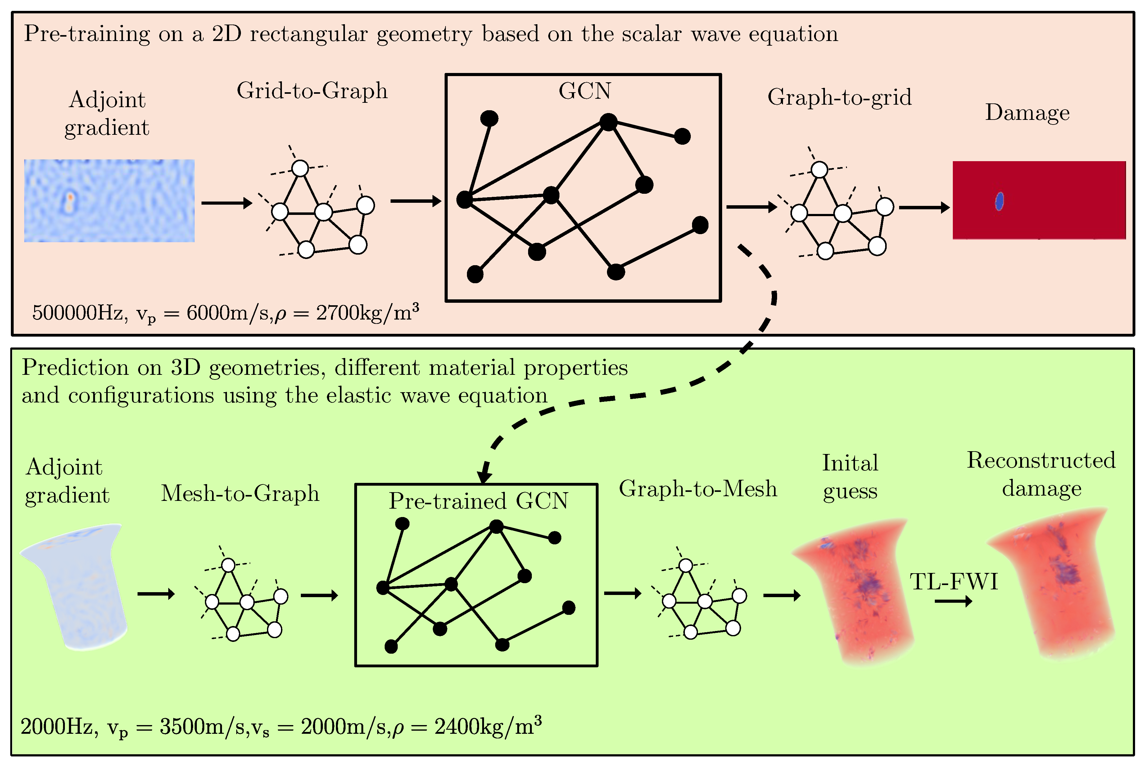
Figure 2.
Representation of a meshed object into a graph. The density scaling function is defined as the features of the nodes of the graph representing the mesh.
Figure 2.
Representation of a meshed object into a graph. The density scaling function is defined as the features of the nodes of the graph representing the mesh.
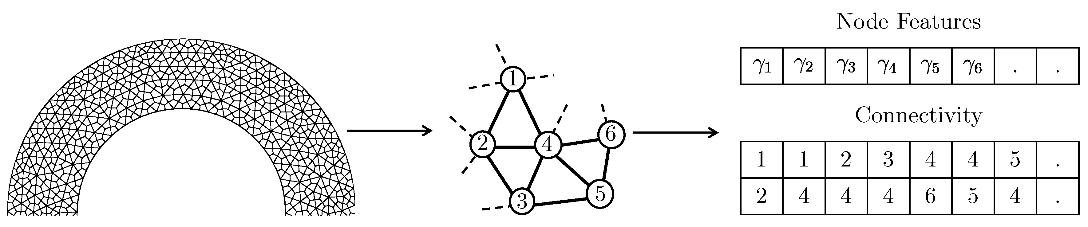
Figure 3.
(a) The raw gradient calculated from the first iteration of a classical FWI undergoes two steps of pre-processing before being used as an input to the GCN. (b) A region of interest is added (shown with black dotted lines), which removes high (and spurious) gradient values in the vicinity of the sensors on the bottom boundary as well as due to reflections from the side and top boundaries. Next, the gradient is normalized using the wavefield, and the gradient values are clipped. Lastly, the gradient (shown on the right) is scaled between -1 to 1.
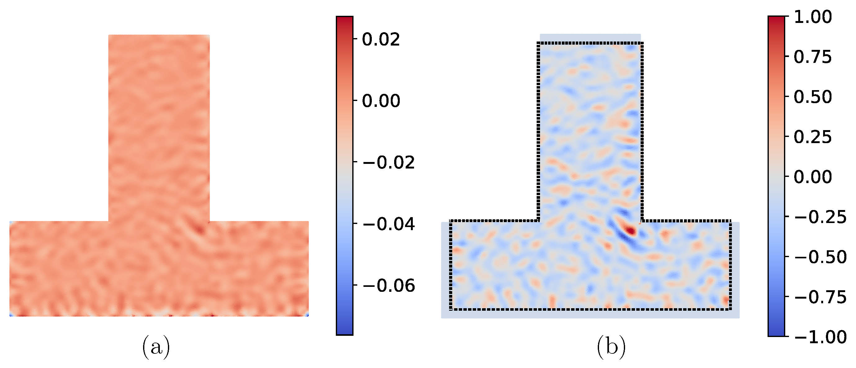
Figure 4.
Representation of a meshed object of arbitrary shape as a graph applied to the TL-FWI using a GCN. The density scaling function is defined as the features of the nodes of the graph representing the mesh.
Figure 4.
Representation of a meshed object of arbitrary shape as a graph applied to the TL-FWI using a GCN. The density scaling function is defined as the features of the nodes of the graph representing the mesh.
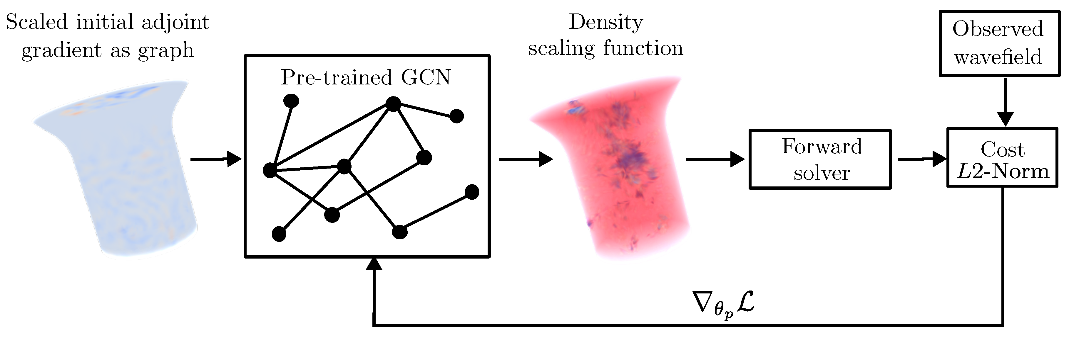
Figure 5.
Comparison of GCN-based TL-FWI with CNN-based TL-FWI.
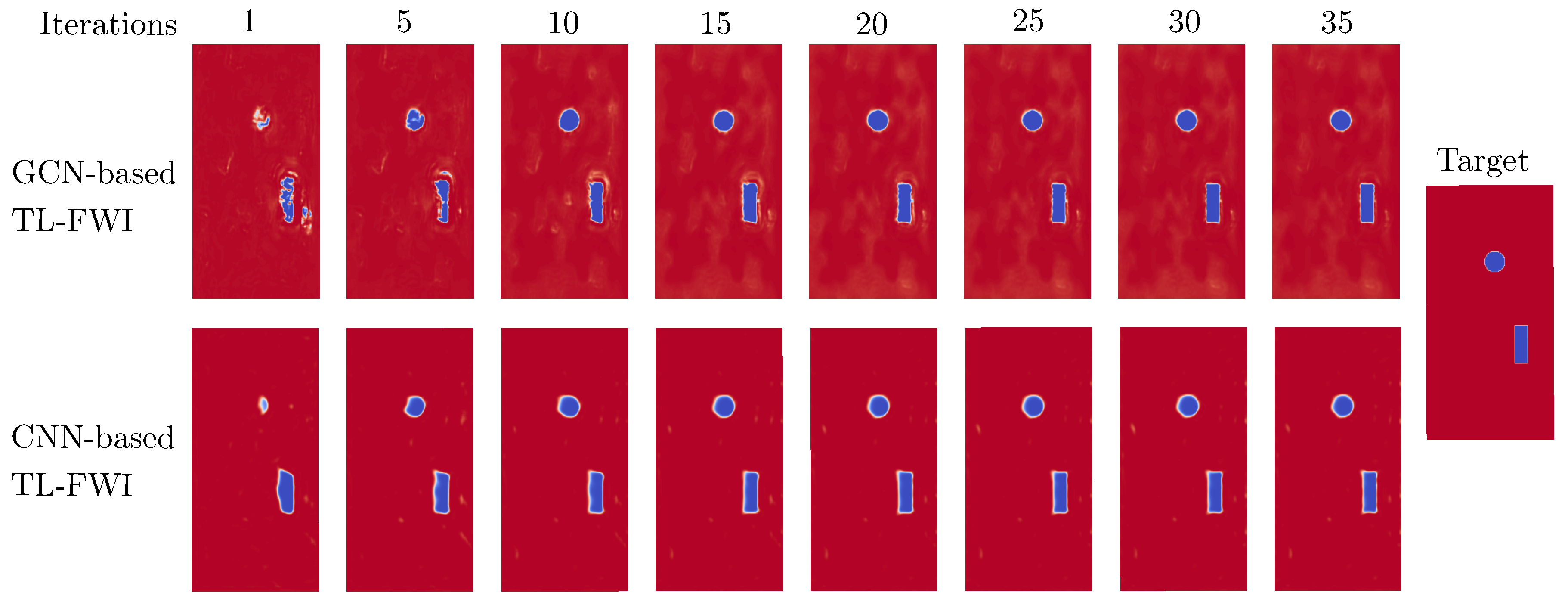
Figure 6.
Comparison of scaling function reconstruction for the T-shaped geometry. The GCN-based TL-FWI approach (c) successfully reconstructs the scaling function much faster and more accurately than the classical FWI approach (d). The runtime of GCN-based TL-FWI is seconds and seconds for classical FWI.
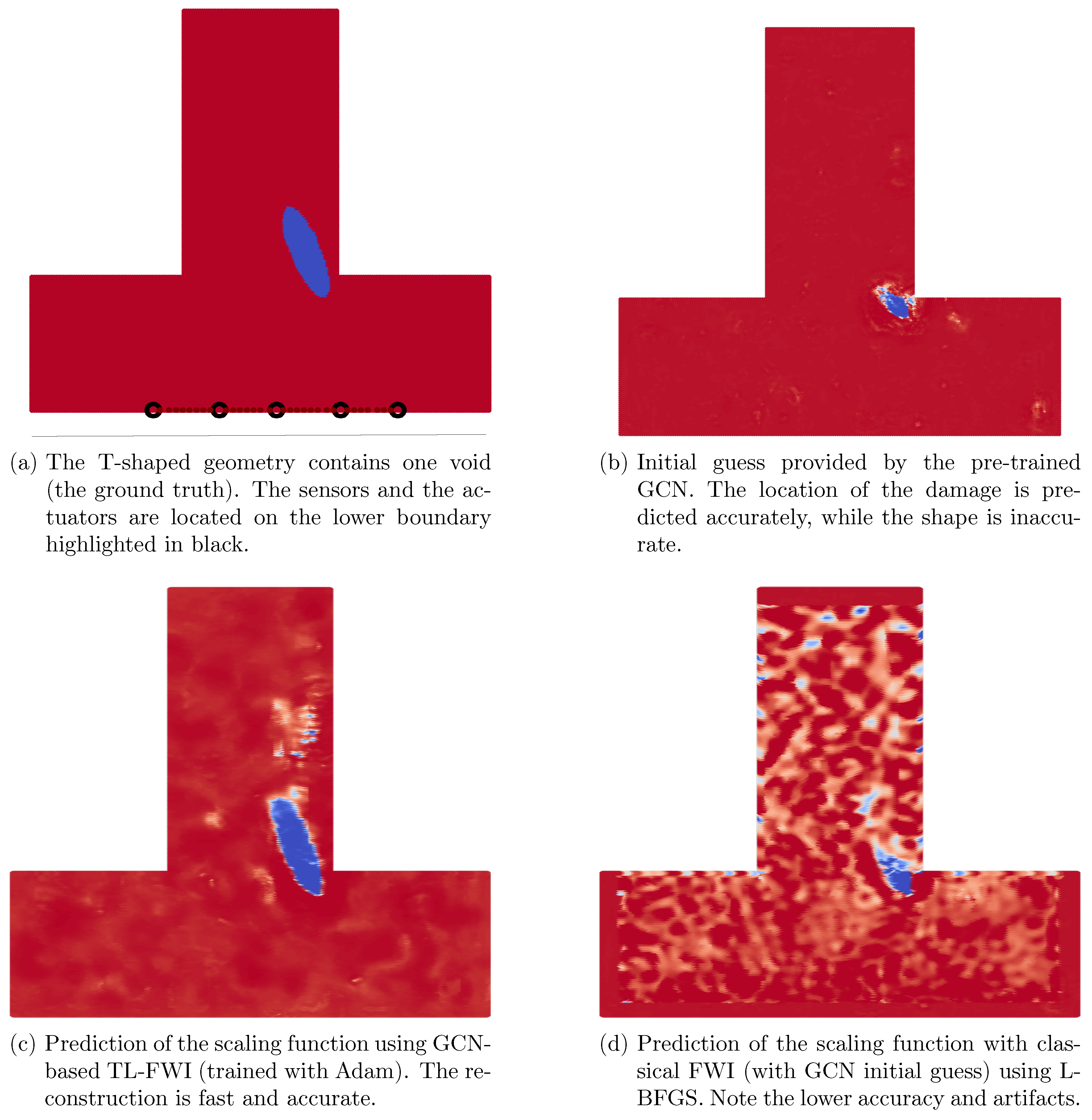
Figure 7.
Comparison of scaling function reconstruction for the T-shaped geometry with three defects and an inaccurate initial guess. The GCN-based TL-FWI approach (c) successfully reconstructs the scaling function faster, more accurately and with significantly fewer artifacts than the classical FWI approach (d). The runtime of GCN-based TL-FWI is seconds and seconds for classical FWI.
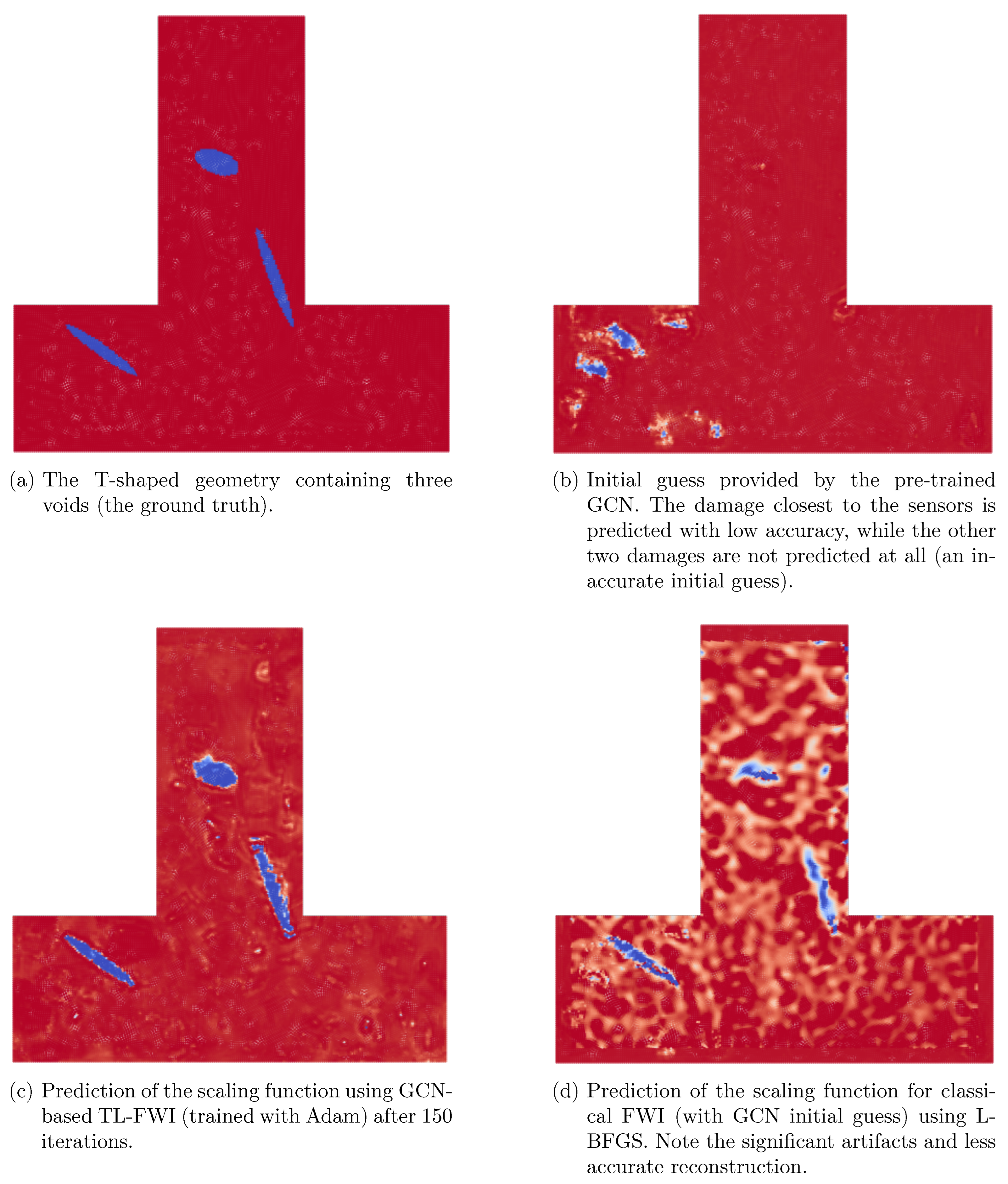
Figure 8.
Point cloud visualization of the flange damage. The opacity of the points is adjusted based on the scaling function values to highlight the low values corresponding to the damage. Comparing the final reconstructions (c) and (d) shows the GCN-based TL-FWI’s superior ability to identify the shape and location of the two elliptical damages. The runtime of GCN-based TL-FWI is 5.5 hours and 13.7 hours for classical FWI.
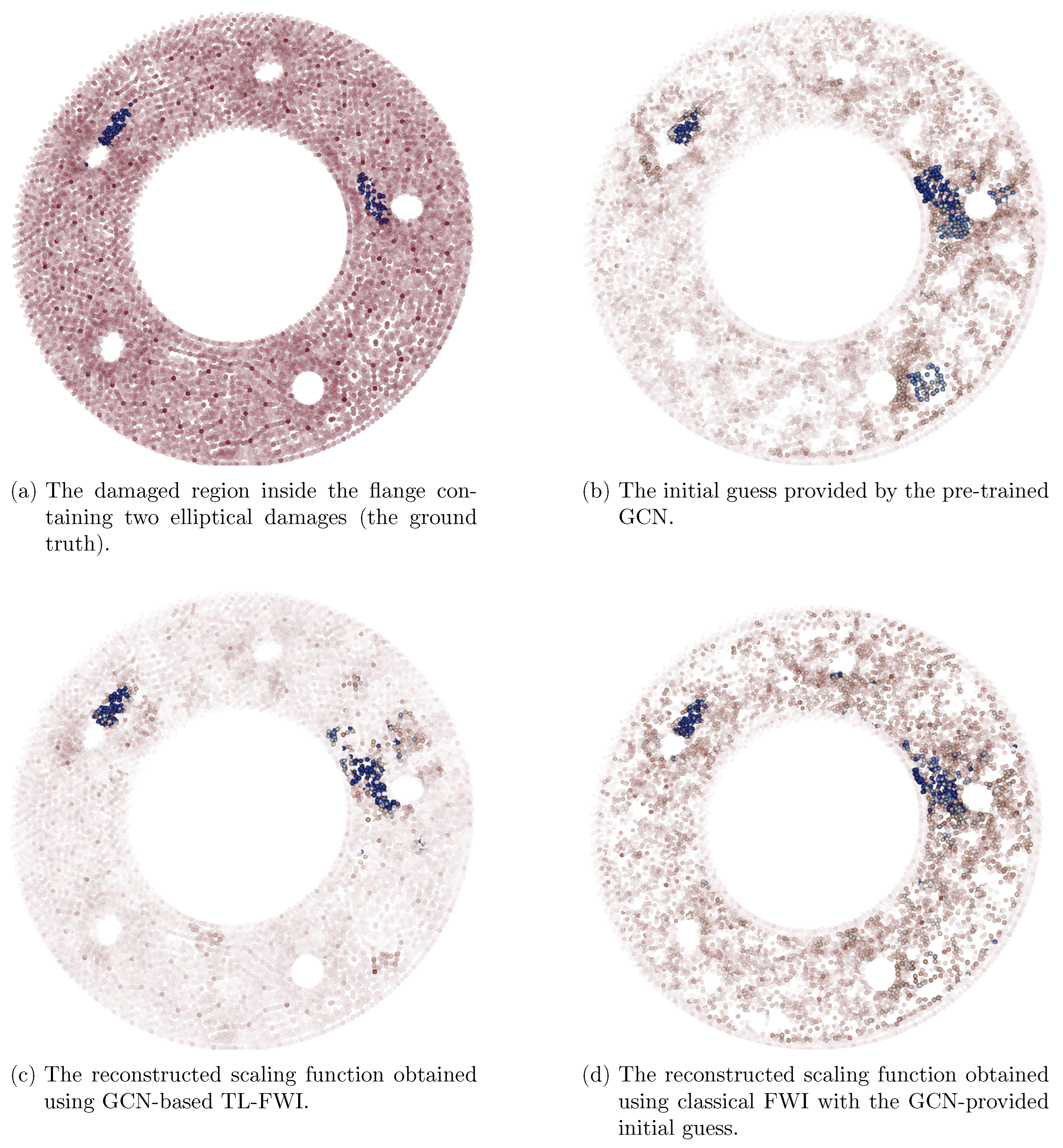
Figure 9.
Point cloud visualization of the cylindrical column damage. The final reconstruction from GCN-based TL-FWI (c) is compared with classical FWI (d). The total computational runtime for both methods was same in this case.
Figure 9.
Point cloud visualization of the cylindrical column damage. The final reconstruction from GCN-based TL-FWI (c) is compared with classical FWI (d). The total computational runtime for both methods was same in this case.
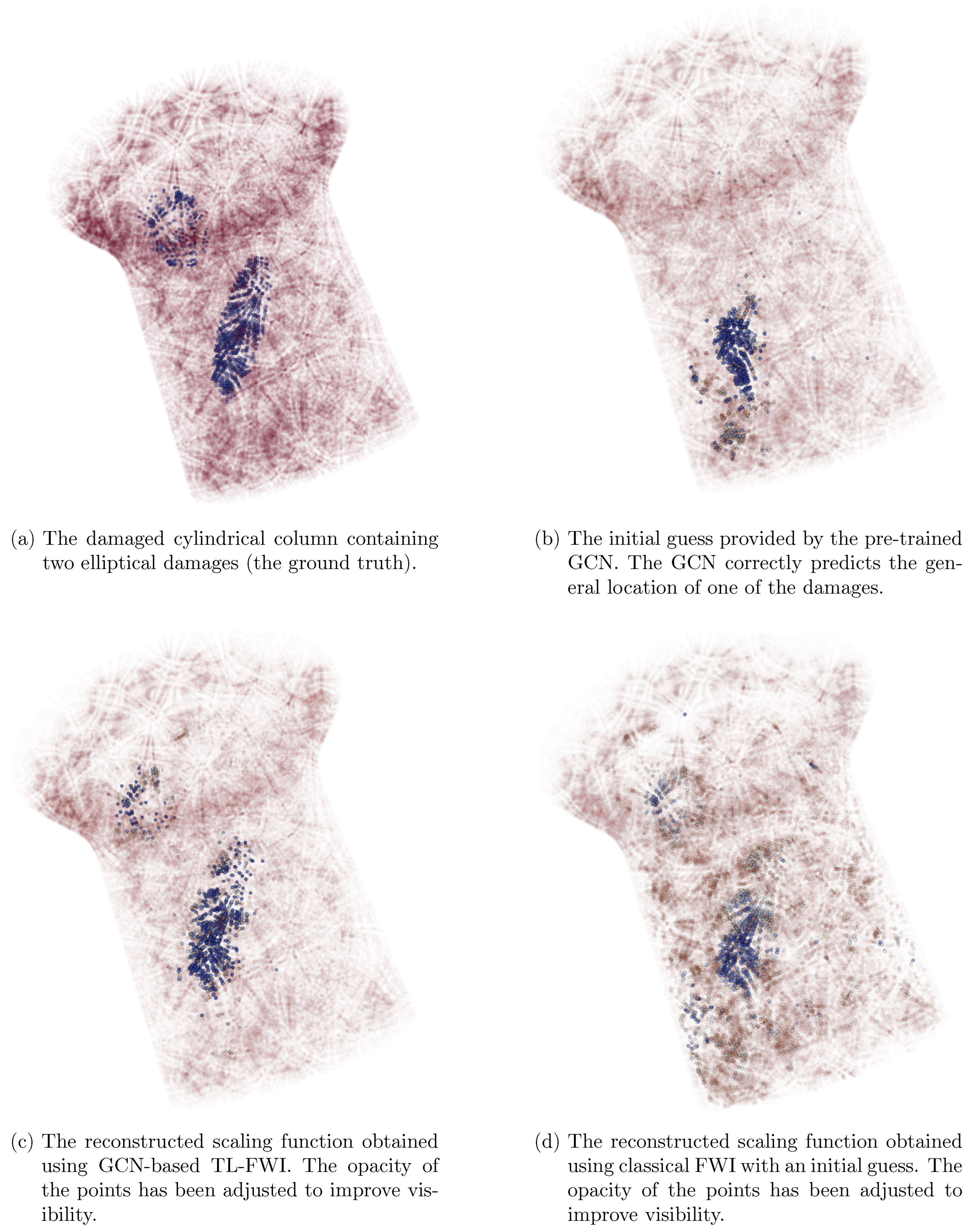
Figure 10.
The influence of the number of neighbor connections on the performance of GCN-based TL-FWI. The figure on the left shows the reduction of cost (normalized) over the iterations for increasing connections. Increasing the number of connections increases the rate of reduction of cost over iterations. The figure on the right shows the Normalized MSE over iterations. Increasing the number of connections beyond a certain limit results in poor reconstruction of the damage (characterized by large MSE values), although the cost is low, indicating higher noise.
| [width=0.49grid=both, xlabel=Iteration,ylabel=Normalized Cost, ymode = log] [color=BlueViolet, thick] file datatikz/costTLFWI15.dat; [color=RosyBrown, thick] file datatikz/costTLFWI2.dat; [color=Peru, thick] file datatikz/costTLFWI25.dat; [color=DarkRed, thick] file datatikz/costTLFWI3.dat; [color=MediumSeaGreen, thick] file datatikz/costTLFWI325.dat; | [width=0.49grid=both, xlabel=Iteration, ylabel=Normalized MSE, legend style=draw=none, nodes=innersep=0.1em] [color=BlueViolet, thick] file datatikz/mseTLFWI15.dat; [color=RosyBrown, thick] file datatikz/mseTLFWI2.dat; [color=Peru, thick] file datatikz/mseTLFWI25.dat; [color=DarkRed, thick] file datatikz/mseTLFWI3.dat; [color=MediumSeaGreen, thick] file datatikz/mseTLFWI325.dat; |
Table 1.
Properties of the simulation for 2D T-shaped geometry
| Property | Value |
|---|---|
| Excitation frequency | |
| Simulation time | s |
Disclaimer/Publisher’s Note: The statements, opinions and data contained in all publications are solely those of the individual author(s) and contributor(s) and not of MDPI and/or the editor(s). MDPI and/or the editor(s) disclaim responsibility for any injury to people or property resulting from any ideas, methods, instructions or products referred to in the content. |
© 2026 by the authors. Licensee MDPI, Basel, Switzerland. This article is an open access article distributed under the terms and conditions of the Creative Commons Attribution (CC BY) license (http://creativecommons.org/licenses/by/4.0/).
Copyright: This open access article is published under a Creative Commons CC BY 4.0 license, which permit the free download, distribution, and reuse, provided that the author and preprint are cited in any reuse.


