Submitted:
11 January 2026
Posted:
13 January 2026
You are already at the latest version
Abstract
Unmanned Aerial Vehicle (UAV), when equipped as communication relays, offer a flexible solution to extend Vehicle-to-Vehicle (V2V) communications beyond fixed infrastructure and Non-Line-of-Sight constraints. In this setting, the allocation of radio resources, across time, frequency and space through beamforming, is challenged by the mobility of Connected and Autonomous Vehicles (CAVs) and their temporal dependencies, as access opportunities depend on prior transmission outcomes such as queue backlog or failed attempts. This paper proposes a Radio Resource Assignment (RRA) framework for UAV-aided V2V networks with beamforming-capable UAV relays. The model discretizes time and space to account for mobility and to track the movement of groups of CAVs across beam segments. The model also incorporates Time Division Multiple Access (TDMA)-based scheduling, beam activation constraints, and realistic traffic generation patterns. Analytical expressions are derived for per-user success probability and system throughput under both, ideal and realistic conditions, and they are validated against simulations, confirming the accuracy of the proposed approximations. Numerical results highlight trade-offs involving UAV altitude and resource allocation interval, while a heuristic beam-activation optimization strategy is shown to further enhance performance, achieving up to 12\% throughput gain over uniform activation.
Keywords:
mobility
; unmanned aerial vehicles
; V2V
; radio resource assignment
; beamforming
1. Introduction
The evolution towards next-generation networks, including Fifth-Generation (5G)-Advanced and Beyond, intend to reshape mobile communications by addressing increasingly stringent requirements in terms of data rate, latency, reliability, and seamless three-dimensional (3D) coverage [1]. Fulfilling this vision requires a fundamental shift in network architecture, exemplified by the growing prominence of Non-Terrestrial Networks (NTNs) [2]. By integrating spaceborne and aerial components with terrestrial infrastructure, NTNs enable global reach, enhanced resilience, and service continuity in areas beyond the coverage of ground-based systems.
Among NTN enablers, aerial platforms such as satellites, High-Altitude Platform Stations (HAPS), and Unmanned Aerial Vehicles (UAVs) are expected to play a key role in delivering adaptive and on-demand coverage. In particular, UAVs stand out for their mobility, reconfigurability, and rapid deployability, making them suitable for dynamic and infrastructure-sparse environments [3]. Their strategic relevance is recognized in 3rd Generation Partnership Project (3GPP) Technical Report 38.811 [4], which highlights UAVs as airborne Base Stations (BSs) or relay nodes capable of extending connectivity under challenging conditions.
For these reasons, UAVs have attracted growing attention in the literature, particularly as aerial relays to support ground users. They offer an effective means of overcoming link blockage, mitigating Non-line of Sight (NLoS) conditions, and enhancing communication reliability [5]. When their role is extended to vehicular network scenarios, UAVs have been employed for tasks such as edge offloading [6,7], congestion mitigation [8], and time-sensitive data dissemination [9]. In such contexts, however, ground-user mobility plays a critical role in communication performance, and accurately capturing its impact remains a major challenge. Resource allocation is often modeled using snapshot-based models, which treat each time instance in isolation [10,11], failing to consider whether a user successfully transmitted a packet or accumulated failed attempts in previous intervals. When mobility is explicitly modeled and vehicles are continuously tracked over time, such memoryless abstractions become inadequate. Instead, the system must account for temporal coupling, whereby each user’s transmission history (e.g., queue backlog caused by prior drops or missed scheduling) influences subsequent resource allocation decisions and access opportunities.
This paper addresses the identified gaps by proposing a mathematical framework for Radio Resources Assignment (RRA) in UAV-assisted vehicular communication scenarios, accounting for mobility. Vehicles generate sensor data, which is transmitted in Uplink (UL) to UAVs hovering at fixed altitudes and acting as relay nodes. Each UAV serves a road segment and subsequently rebroadcasts the received data in Downlink (DL). Directional beams are used for coverage, with activation constrained by the limited number of available Radio-Frequency (RF) chains. Inter-beam interference is assumed to be negligible [12], while intra-beam access is managed through a Time Division Multiple Access (TDMA)-based scheduling scheme, with resource allocation decisions updated at fixed intervals.
The proposed model captures (i) the mobility of vehicles from their entry to their exit within an highway segment covered by UAVs; (ii) UAV beam layout and activation constraints imposed by hardware limitations; (iii) wireless channel conditions, characterized by the UAV-to-vehicle Signal-to-Noise-Ratio (SNR); (iv) communication parameters such as bandwidth and numerology; (v) traffic density and (vi) different data generation patterns. Crucially, the framework preserves the state of each vehicle’s transmission buffer, allowing for temporally consistent resource allocation decisions that account for packet backlog and retransmission history.
Validated through simulation, the framework supports performance evaluation, via success probability and user/network throughput, and optimization of RRA. Specifically, it enables joint tuning of UAV’s altitude and resource allocation interval, and the selection of the optimal beam activation pattern under RF constraints maximizing a chosen performance metric.
The remainder of the paper is organized as follows. Section 2 outlines the related work and highlights the novel contributions of this study. Section 3 introduces the system model, while Section 4 details the resource allocation mechanism. Section 5 describes the user mobility model and the adopted traffic generation patterns. The problem formulation is then developed in Section 6, first under ideal assumptions in Section 7, and subsequently extended to a more realistic scenario in Section 8. Section 9 presents the numerical results and performance evaluation, and finally, Section 10 concludes the paper.
2. Literature Review
The use of UAVs as enablers of wireless connectivity has attracted growing attention in recent years. Many works have investigated their role as aerial relays, with efforts primarily focused on optimizing deployment strategies, relay selection, and resource allocation, or joint combinations of these dimensions, to serve ground users efficiently.
For instance, in [13], relay selection and scheduling are jointly optimized in a UAV-assisted Millimiter-Wave (mmWave) network to minimize transmission time, through a two-step random scheme and a dynamic strategy that avoids relay contention. A similar objective is pursued in [14], where a Reinforcement Learning (RL) approach based on proximal policy optimization and deep Q-networks is employed to cope with blockage-prone conditions. In [15], UAV placement, bandwidth, and power allocation are jointly optimized in public safety scenarios to maximize the utility of video streams under practical system constraints. A different direction is explored in [16], which introduces a hierarchical matching algorithm to coordinate relay selection within UAV clusters, enabling stable user grouping and efficient task offloading to edge servers.
Several contributions specifically target UAV-assisted vehicular communication scenarios. For example, [17] proposes a blockchain-based coordination mechanism for spectrum and power allocation among UAVs to reduce latency under interference constraints. In [18], a cooperative strategy is proposed in which UAVs assist congested Road Side Units (RSUs) to mitigate interference and improve throughput. In [19], the challenge of ensuring timely delivery of sensor data in vehicular networks is addressed by jointly optimizing UAV trajectories and UL scheduling. A comprehensive performance analysis for UAV-assisted vehicular sidelink communications is presented in [20], which accounts for beamforming design, traffic load, and deployment parameters.
However, mobility, an inherent feature of vehicular networks, remains a challenging dimension to incorporate effectively into mathematical frameworks that aim to model the behavior of UAV-enabled communication systems. While several studies attempt to incorporate user dynamics, key limitations persist in how mobility influences resource allocation decisions. In [21], a mobility-aware offloading algorithm is proposed for UAV-assisted vehicular edge computing, where predictive models estimate vehicle positions to adapt offloading strategies. In [22], UAVs act as mmWave BSs under a joint optimization of deployment, association, and spectrum allocation, relying on predefined mobility models. The effect of user mobility on network performance is highlighted in [23], where adaptive update intervals for UAV repositioning are introduced. In [24], user mobility levels guide UAV trajectory adaptation and resource partitioning between sensing and communication. [25] and [26] exploit mobility information to optimize UAV energy consumption and joint trajectory-power strategies, respectively. While these contributions mark important progress, they exhibit two main limitations. First, in works such as [22], mobility is often incorporated as a static input (i.e., movement patterns are considered in aggregate, rather than capturing the real-time, slot-by-slot evolution of each vehicle). Second, although other studies do adapt UAV behavior dynamically based on user movement (e.g., through trajectory reconfiguration or update intervals), they lack a state-tracking mechanism capable of modeling per-user queue evolution, transmission history, and access retries.
To the best of the authors’ knowledge, this is the first work to introduce a mathematical framework that explicitly captures the dynamic interplay between vehicle mobility, queue states, and communication constraints. Our contribution departs from existing literature in two key aspects:
- Temporal coupling and queue awareness, achieved through a time-evolving model that tracks each vehicle across successive time slots, preserving internal states such as queue content and retransmission history. This allows the resource allocation process to account for the outcome of previous transmissions, ensuring a temporally consistent and fair system behavior;
- Realistic traffic modeling, by incorporating heterogeneous data generation patterns, including periodic event-driven transmissions and probabilistic schemes where new packets are generated as soon as the transmission queue is emptied. This enables the framework to reflect both sporadic and continuous communication behaviors typical of Vehicle-To-Everything (V2X) applications [27].
3. System Model
3.1. Reference Scenario and Application
Let us examine the Vehicle-to-Vehicle (V2V) communication scenario supported by UAVs, as illustrated in Figure 1. In this setting, Connected and Autonomous Vehicles (CAVs) travel unidirectionally along a highway segment with a total length, L, moving at a constant speed, v, from point A to point B. The highway is covered by a fleet of UAVs hovering at a fixed altitude, h, above ground level. These UAVs are deployed at a constant inter-drone distance, . Each UAV covers a specific road segment of length using multiple beams. The antenna system onboard each UAV is configured as a hybrid digital Uniform Linear Array (ULA), comprising antenna elements and RF chains, which determines the number of simultaneously active beams. Similarly, each CAV is equipped with a ULA consisting of antenna elements and a single RF chain.
Through onboard sensors, each CAV collects environmental data, which is encapsulated into packets of size D [bits] that should be transmitted to other CAVs in the network to support extended sensing applications [28]. These applications enable vehicles to share locally gathered data with nearby vehicles, enhancing their environmental awareness beyond their own sensing capabilities. To ensure robust and reliable communication, even in blockage scenarios [5], we envisage the integration of UAVs as relays to facilitate efficient information dissemination among CAVs.
The data transmission process consists of two phases: an UL phase, where the CAV sends the data packets to the UAV responsible for its current road segment, and a DL phase, during which the UAV broadcasts the data to other CAVs. In this work, we focus exclusively on the UL direction, As the network is collecting sensors data, the traffic requirements are particularly challenging for the UL communication [29].
3.2. Beamforming and Path Loss Model
The UAVs employ a beamforming codebook , whose cardinality determines the number of beams used for ground coverage. Throughout the paper, we adopt a Discrete Fourier Transform (DFT) codebook, as in [30], which guarantees full coverage with the minimum number of beams. Each beam covers a ground footprint of length , with , determined using the methodology in [20]. As a result, the total coverage extent provided by a single UAV is given by
The strategic placement of the UAV ensures a reliable ground-to-aerial communication link without obstructions. The path loss in dB experienced by a generic CAV within the bth beam is modeled following [31] and it is assumed to be uniform across the entire beam [20]:
where denotes the distance between the barycenter of the bth beam footprint and the UAV, and denote the excess path loss offset and the path loss exponent, respectively, while is a Gaussian random variable, with variance , modelling the shadowing component.
4. The Radio Resource Assignment Process
Similarly to the 5G NR Standard [32], we assume that each communication instance occurs in a predefined time-frequency resource. In addition, we exploit the spatial dimension, via the use of beamforming, where the association between beams and CAVs can be established during the initial access procedure as in [33]. We also assume negligible inter-beam interference, allowing CAVs covered by different beams to reuse the same time-frequency resources [29]. Conversely, to avoid intra-beam interference, different Resource Units (RUs) must be assigned to different CAVs within the same beam. To this end, a TDMA protocol is implemented in each beam, b, whereby time is divided into frames, each of duration , activated sequentially. Since each beam spans a ground footprint of length , the number of TDMA frames per beam is given by
We define as the set of spatial segments composing beam b, and as the corresponding set of time frames:
During each TDMA frame of duration , the RRA algorithm, running at the UAV, assigns UL resources to the CAVs located in the corresponding spatial segment of the beam (see Figure 2). In particular, and is the road segment crossed by a CAV during a single frame.
We now derive the number of CAVs that can be served concurrently in a frame, assuming RUs are available. According to 5G, in the frequency domain, a Physical Resource Block (PRB) consists of subcarriers with subcarrier spacing, , determined by the selected 5G numerology. The bandwidth of a single PRB is then given by
With PRBs allocated to a communication channel, the total channel bandwidth is given by
The channel capacity, , can be calculated using the Shannon capacity formula as per [34]:
where is the minimum SNR required for reliable communication.
In the time domain, a PRB is defined over a time slot, , which corresponds to the transmission of 14 Orthogonal Frequency-Division Multiplexing (OFDM) symbols [35]. Hence, the capacity of a single RU, combining both time and frequency dimensions, is expressed as
The number of RUs allocated to the UL direction during a resource allocation interval of duration , is given by
where B is the total bandwidth available in a beam. The number of RUs required to meet the traffic demand D can be computed as
Finally, the maximum number of CAVs that can have the required number of resources assigned during a single interval can be computed as follows:
where the floor function, , ensures the result is an integer number.

Table 1.
General notation description.
| Symbol | Description | Symbol | Description |
|---|---|---|---|
| Number of serving UAVs | Number of available beams | ||
| Number of RF chains | RRA interval duration | ||
| k | Time interval index | Total traversal time intervals | |
| ℓ | Beam index | Travel time from A to B | |
| Spatial segments in beam ℓ | TDMA frames in beam ℓ | ||
| v | Vehicle speed | U | Maximum servable vehicles per RRA interval |
| Beam traversal intervals | Minimum discretized road segment length | ||
| M | Maximum number of vehicles per segment () | Vehicle length | |
| Probability of a vehicle in slot | Vehicle density | ||
| Average vehicles per segment () | Packet generation probability at interval k | ||
| Minimum packet generation probability | Maximum packet generation probability | ||
| T | Period between consecutive packet generation events | CAVs with queued packet | |
| CAVs without queued packet | Accessing CAVs | ||
| Successful CAVs | Failed CAVs | ||
| Average CAVs with queued packet | Average CAVs without queued packet | ||
| Average accessing CAVs | Average successful CAVs | ||
| Average failed CAVs | Probability of having a queued packet | ||
| Probability of newly generated packet | Connection probability | ||
| Activation probability | Blocking probability | ||
| SNR threshold | Average SNR in the ℓth beam | ||
| Mean of average SNR in beam ℓ | Standard deviation of average SNR in beam ℓ | ||
| Average success probability | Success probability | ||
| Network throughput | Average user throughput |
5. Traffic Model: Mobility and Data Generation
5.1. Notation
Henceforth, the beams covering the road segment from A to B, served by UAVs (each providing beams), are indexed as . Time is discretized into RRA intervals of duration , with each interval indexed by , where is the total number of intervals required for a CAV to traverse the road segment from A to B. Specifically, , where is the travel time from A to B, given by . Equivalently, can be expressed as , in accordance with Equation (3). Finally, let denote the set of discrete intervals required to traverse the ℓth beam.
5.2. CAVs Mobility and Distribution
In this work, we assume each represents a discrete snapshot of the scenario, during which vehicles occupying the same move together to the next segment. Since the RRA process operates at intervals of , this ensures synchronization between resource allocation and the vehicle’s movement. The maximum number of vehicles that can fit within is given by , where represents the physical size of the CAV and allows for a minimum safety distance, assuming the scenario of maximum traffic congestion [36]. Assuming a Point Poisson distribution over a single road segment, the probability of having exactly n vehicles within follows a Binomial distribution [20]:
where represents the probability of finding a vehicle in a given road segment of length , given by
with the vehicle density [car/km].
Now, considering the number of vehicles entering the scenario in the first frame duration, that is moving in the first road segment of the first beam, it is still Binomially distributed, with average, , given by
5.3. Data Generation Model
In the following, we introduce two distinct traffic models that capture the packet generation logic of CAVs as they traverse the road segment from point A to point B. We will denote as the probability that a CAV can generate a new packet in frame k.
5.3.1. Probabilistic Traffic Model
In this setting, we assume that packet generation occurs randomly, governed by an underlying stochastic process. In particular, the value of is not constant; rather, it evolves over time to reflect the dynamics of V2X messaging, where transmission periodicity adapts to changes in the vehicle’s state, as observed for Cooperative Awareness Messages (CAMs) [37,38]. In the remainder of this section, we introduce two time-dependent functions that model this evolution and serve as candidate patterns for packet-generation probability.
- Parabolic traffic pattern. In this scenario, each CAV entering the system at point A is assumed to have an initial queued packet with probability . As the vehicle traverses the road segment and successfully transmits its queued packet, the probability of generating a new packet increases progressively, reaching a maximum value, , at the midpoint of the segment (i.e., when ). Thereafter, the packet generation probability decreases, reverting to by the time the vehicle reaches point B (i.e., at ). The expression governing is then given bywhere .
- Linear decreasing traffic pattern. In this case, vehicles entering the system have a queued packet with probability . As they progress along the road, the probability of generating a new packet (once their queue is cleared) decreases linearly, reaching by the time they arrive at point B. The function governing this evolution is given bywith .
5.3.2. Periodic Traffic Model
In this scenario, vehicles generate a packet either upon entering the system or at periodic intervals triggered by a specific event. Accordingly, is defined as
where T denotes the time interval between two consecutive packet generation events. This interval corresponds to the time required for all CAVs to empty their queues, which is influenced by both vehicle density and UAV resource availability.
6. Mathematical Model Overview
This section introduces the key components of the proposed mathematical framework developed to model the traffic dynamics of CAVs traversing a road segment from point A to point B, covered by UAVs, while attempting to transmit their UL traffic demands in support of V2V applications. The proposed scheme captures vehicle mobility by tracking groups of vehicles across intervals, considering those that enter simultaneously and occupy the same segments. Built on this logic, the scheme accounts for the cumulative effect of previous allocation intervals, making the outcome at any given time dependent on past decisions, thus introducing a temporal dependency that increases the overall complexity.
6.1. Notation
The following notations will be used:
- : the number of CAVs with a data packet queued for transmission. This condition occurs when (i) a new packet is generated following a successful transmission1, or (ii) a previous transmission has failed and the same packet must be retransmitted. Conversely, denotes the number of CAVs without a packet in the queue;
- : the number of CAVs attempting to access resources, i.e., vehicles that (i) have a packet in the queue, (ii) are connected to the UAV, (iii) are located within an active beam, and (iv) occupy a segment during a frame k that is activated according to the TDMA procedure outlined in Section 4;
- : the number of CAVs that successfully receive resources to transmit their data;
- : the number of CAVs that did not succeed in receiving resources to transmit their data.
All of the above random variables may depend on the considered time frame k and the beam ℓ. Therefore, they will be denoted as when appropriate. As will be clarified later, these variables follow a Binomial distribution. Their expected values, denoted as , , , , will be derived in the following sections.
Other notations are:
- : probability that a CAV has a packet in the queue, which occurs if (i) a new packet has been generated after a successful transmission (we denote this probability ), or (ii) a previous packet remains in the queue because the last transmission attempt failed;
- : connection probability, that is the probability that a CAV is connected to the UAV, that is it has an SNR above the threshold;
- : activation probability, that is the probability that a CAV is (i) within an active beam and (ii) located in a road segment during a frame k that is active according to the TDMA procedure;
- : blocking probability, that is the probability that a CAV does not have RUs assigned in a given .
As for the case of the random variables defined above, these probabilities may depend on the considered time frame k and on the beam ℓ.
6.2. Connection Probability
In the following, we compute the probability that a CAV in the ℓth beam is connected to the UAV, which corresponds to the event that the UL SNR of the CAV-UAV link exceeds the threshold , defined as the minimum value required to satisfy the system’s Quality of Service (QoS) constraint.
For analytical tractability, we adopt the uniform-SNR assumption within each active beam, as in [20]. Accordingly, all CAVs served by the same beam are assumed to experience the same SNR. Under this assumption, the connection probability is given by
where denotes the average SNR in the ℓth beam. By the central limit theorem, the distribution of the average SNR in dB can be approximated as , where the mean value is computed using the path loss model in Equation (2), and the standard deviation is [29,39]. Hence, the connection probability in beam ℓ can be expressed as
where is the Q-function.
6.3. Activation Probability
We now derive , which represents the probability that, in a given frame, a CAV is illuminated by an active beam and that the frame is active from the TDMA protocol perspective, as described in Section 4. Regarding beam illumination, when , only a subset of beams can be active simultaneously. Consequently, if a vehicle is traveling under an inactive beam, it remains unserved and is excluded from resource assignment during that resource allocation interval. Concerning the TDMA protocol employed within each beam, a different road segment of length is sequentially illuminated and served during each frame k of duration . Since a CAV needs intervals to traverse the ℓth beam, it is, on average, allocated UL resources in one out of every frames during its traversal. Therefore, can be computed as
where the first term accounts for the beam activation state and the second one for TDMA. The second term clearly highlights how larger beams exacerbate the impact of the TDMA scheme, as they require longer traversal times, i.e., higher values of , which in turn lead to a lower activation probability .
6.4. Blocking Probability
Finally, we derive the blocking probability, , using the Erlang-B formula [40], , as
where U is the maximum number of vehicles that can be accommodated in a given RRA interval (as defined in Equation (11)), and represents the average number of vehicles attempting to access resources in that interval. The Erlang-B formula can be recursively computed as
by setting .
6.5. Target Performance Metrics
In the following, we introduce the performance metrics derived in the remainder of the paper and evaluated in the numerical results.
6.5.1. Success Probability
The success probability for a CAV in frame k while traversing beam ℓ, denoted , is the probability that all of the following conditions are satisfied simultaneously: i) the CAV has a queued packet ready for UL transmission; ii) the CAV is connected to the UAV; iii) beam ℓ and time frame k are active, and iv) the CAV receives sufficient resources to transmit D bits in the UL. Therefore, it is given by
with , where we account for the contention among CAVs competing for the available resources.
6.5.2. Average Success Probability
The average success probability, averaged over the entire travel of the CAV along the road, is given by
where the denominator expresses the total probability of generating new packets along the entire path.
6.5.3. Average User Throughput
The average user throughput achieved by a CAV during a generic frame k, is given by
6.5.4. Network Throughput
The overall network throughput generated by all CAVs traversing the road segment from A to B over a time period of time slots, is given by
where denotes the average number of users that fit within a spatial slot of length , as defined in Equation (14).
7. Mathematical Model Under Ideal Conditions
To simplify the analysis, we first model the traffic evolution under ideal conditions, where and . This implies that i) all CAV-UAV links maintain an SNR level above the threshold , ii) all beams are continuously active (i.e., ), and iii) the TDMA scheme is not applied within each interval for that beam. Under these assumptions, , and all variables will only depend on k and not on ℓ.
As anticipated in Section 6, all the random variables defined and considered in this work follow a Binomial distribution, as they result from a sequence of independent thinning operations applied to the initial binomial population n introduced in Equation (12) [41]. This modeling assumption holds under the condition that the maximum number of CAVs M fitting within a segment is fixed and known and that each thinning step (e.g., determining whether a CAV has a queued packet, is successfully served, or not) is governed by a constant and independent probability within each considered frame k. In the remainder of the paper, we focus exclusively on average values, which allows us to preserve analytical tractability while maintaining the binomial structure in expectation.
7.1. Probabilistic Traffic Model
We first derive and under the probabilistic traffic model outlined in Section 5.
7.1.1. Deriving
The initial values at time step are given by
where the first two equations account for the fact that a CAV generates a new data with probability , and the last two equations take into account that CAVs have success in getting resources with probability .
Then, in the second time frame, , we have:
where the first equation accounts for the fact that a new packet may be present in the queue either because the queue was initially empty, or the previous packet was successfully transmitted, or due to a previously failed transmission. The second equation accounts for the case where no packet was in the queue, or no new packets are generated. The last two equations follow the same derivation as in the case . By generalizing, we have:
7.1.2. Deriving
To simplify the notation, we introduce the following probabilities: (i) , i.e., the probability that no data is present in the queue; (ii) , i.e., the probability of a successful transmission, conditioned on the presence of data in the queue, and (iii) , i.e., the probability of a failed transmission, also conditioned on the presence of data in the queue. The initial values at time step are then given by
Then, generalizing, we have:
7.2. Periodic Traffic Model
We now derive and under the periodic traffic model, where vehicles enter the scenario with a packet already queued.
7.2.1. Deriving
Using the same approach adopted in the probabilistic traffic model, we derive for the case and , with , as follows:
where we account for the fact that, at time steps or , the packet generation probability is . This reflects the synchronous behavior of all n CAVs that entered the system during the same kth interval: upon completing the transmission of their previous packet, each vehicle generates a new one, thereby resetting to its initial value, n.
Then, for the other values of k we have , therefore:
where the first equation accounts for the fact that CAVs have data in the queue only if they failed at the previous attempt (in case of success no new data is generated until the end of the period).
7.2.2. Deriving
Following the same approach used for the probabilistic traffic, and accounting for the values of , we have:
where .
Taking into account the new data packet generation, we have:
8. Modeling in Realistic Conditions
We now relax the assumptions on and , resulting in having and the dependency of these random variables on both beam ℓ and time frame k. Therefore, in the following we derive , , and built upon the previously established expressions for , and (given in Section 7).
Two separate cases are analyzed, that are and .
- For , the average number of vehicles attempting to access resources, accounting for the queue status, the CAV connection, and both beam and time slot activation, is given bywith . Similarly, .
-
For , we first show the specific cases for and to illustrate the underlying logic, and then generalize the derivation ∀ℓ>1.When , the expression of the average number of CAVs attempting to access resources is given bywith k. Equation (37) is expressed as the sum of two contributions corresponding to distinct scenarios that may occur during the traversal of the preceding beam (): (i) if < and beam 1 is not included in the active set, or if <, then the average number of vehicles attempting to access resources in beam 2 during the kth interval is equal to the average number of vehicles that entering the system with a queued packet and that were not served while traversing beam 1 with probability ; (ii) if beam 1 is active and >, then the vehicles contending for resources in beam 2 are those that, over the intervals , attempted to transmit their UL packets with probability . Similarly, .
By generalizing to an arbitrary beam , the final expression for , which captures the cumulative effect of all preceding beams and their states, is given in Equation (39), with and . The term appearing in this formulation is defined by Equation (29) for probabilistic traffic and by Equation (33) for periodic traffic. Likewise, the expression for is reported in Equation (40), where follows Equation (31) or Equation (34), depending on the traffic model. Finally, can be derived by using Equation (40) and substituting to , where is given by Equation (31) for the probabilistic traffic and by Equation (35) for the periodic traffic.
9. Numerical Results
This section presents numerical results evaluating the performance of the proposed mathematical model under realistic conditions for both periodic and probabilistic traffic models. The analysis focuses on the performance metrics introduced in Section 6.5. To assess the accuracy and validity of the mathematical model, a dedicated simulator was developed in the MATLAB environment, using the input parameters summarized in Table 2. The main differences between the simulation and the analytical model are the following. The analytical model assumes a uniform average SNR for all vehicles within the same beam, while the simulator explicitly accounts for the instantaneous SNR experienced by each CAV with respect to the UAV, which is computed according to the formulation provided in Appendix A. Moreover, while the analytical model relies on average quantities, such as , the simulation treats the number of vehicles entering the scenario as the outcome of a realization drawn from a Binomial distribution, as defined in Equation (12). To ensure statistically significant results, the simulation is repeated over Monte Carlo iterations, and performance metrics are averaged across all realizations.
The study evaluates system performance under different UAV altitudes and multiple values of , which represents the duration of the UL resource allocation time frame. Specifically, we consider UAV heights of , 120, and 180 m, and values of 300, 500, 700, and 900 ms. Finally, the number of RF chains is set to , which corresponds to the number of available beams (), thereby allowing all beams to be simultaneously active. As a result, the activation probability is solely influenced by the TDMA scheduling effect, as outlined in Equation (20). The case of is addressed in B.
In Figure 3 is shown the average success probability, , in the case of periodic traffic for a CAV traversing the path from point A to point B. The analytical results exhibit a close match with the simulation outcomes, confirming the validity of the model under the simplifying assumptions introduced at the beginning of this section. The plot shows three continuous curves, each corresponding to a different UAV altitude: 60 m (dark gray), 120 m (medium gray), and 180 m (light gray). The x-axis reports four values of (300 ms, 500 ms, 700 ms, and 900 ms), while the y-axis indicates the average success probability. As the UAV altitude increases, decreases due to lower values of both connection and activation probabilities, i.e., and . Specifically, decreases as a result of higher path loss at increased altitudes, while the broader UAV footprint causes each beam footprint to expand. As increases and remains fixed, the number of intervals required to span the beam also increases, thereby exacerbating the impact of the TDMA effect. Examining the impact of increasing for a fixed height reveals a generally positive effect on . As grows, more resources become available within each RRA interval, and the influence of TDMA allocation in each beam is reduced. As a result, increases, effectively balancing the higher user contention associated with larger , and thus , values.
Figure 4 reports the average user throughput, , achieved by a CAV during a single interval. The plot adopts the same configuration as Figure 3 and, consistently, exhibits a similarly close agreement between the model and simulation (under the assumptions discussed earlier). As expected, decreases with increasing UAV altitude, consistent with the trend observed for . However, unlike the success probability, which continues to grow with larger values, increases up to ms and then begins to decline for longer intervals. The maximum throughput is attained at m and ms. A similar behavior is observed at higher altitudes, although the effect is less pronounced, indicating that the throughput sensitivity to diminishes as the UAV height increases. This reveals a fundamental trade-off in resource allocation. The throughput metric shows that while larger values improve success probability, they also reduce the number of transmission opportunities. The optimal ms balances these competing effects: below this value, gains in success probability dominate; above it, the reduced transmission frequency outweighs further success probability improvements.
The results for the CAV’s average success probability and average throughput under the probabilistic traffic model are omitted, as they exhibit the same trends observed in the periodic case.
To highlight the differences between the two traffic models, Figure 5 illustrates the average throughput achieved by a CAV, , as a function of the total traffic it generates, denoted by G. The latter is computed by multiplying the packet size D by the sum of the probabilities across all beams and time frames. Two UAV heights are considered: 60 m (solid curves) and 120 m (dashed curves). Dark gray, medium gray, and light gray denote the periodic, linearly decreasing, and parabolic traffic models, respectively. Each point along the curves corresponds to a different duration (300, 500, 700, and 900 ms), represented by progressively lighter shades of gray from left to right.
The analysis reveals three key observations. First, consistent with Figure 4, the throughput decreases as UAV height increases from 60 m to 120 m for all traffic models resulting in two distinct groups of curves: upper curves (60 m) and lower curves (120 m), reflecting the degraded channel conditions at higher altitudes and the greater TDMA impact.
Second, the relationship between and generated traffic G shows an inverse correlation: smaller values result in higher traffic generation due to more frequent transmission opportunities, while larger values reduce traffic generation frequency. However, the throughput performance exhibits a non-monotonic behavior with respect to . For all traffic models, ms achieves the peak throughput, representing the optimal balance between resource availability per frame and TDMA effect. As already discussed for Figure 4, values below 700 ms suffer from insufficient resources per frame and increased TDMA impact, while values above 700 ms, despite providing more resources per transmission frame and reduced TDMA impact, result in lower overall traffic generation due to less frequent transmission opportunities. Moreover, larger values correspond to larger segments accommodating more users within the same allocation period, potentially leading to increased contention.
Third, for equivalent traffic loads G, the periodic traffic model achieves lower throughput compared to the probabilistic models (both linear decreasing and parabolic). This performance gap stems from the fundamental difference in packet generation mechanisms. In the periodic traffic model, vehicles can only generate new traffic when all other vehicles within the same have cleared their queues, creating synchronized regeneration cycles with enforced waiting periods. This synchronization constraint limits both the traffic generation rate and transmission opportunities, as vehicles must remain idle until the collective transmission process is complete. Conversely, in the probabilistic traffic model, each CAV regenerates packets immediately upon completing its own transmission, independent of other vehicles’ queue status within the same . This asynchronous approach enables continuous traffic generation and transmission without forced idle periods. As a result, as evident from Figure 5, for equivalent time allocation intervals , the probabilistic models consistently achieve both higher traffic generation loads and superior throughput performance compared to the periodic model. The synchronized waiting periods inherent in the periodic model create temporal inefficiencies that limit both the amount of traffic generated and the rate at which it can be transmitted, resulting in the observed performance gap between the two traffic generation approaches.
An overarching insight from the numerical results is that the activation probability plays a central role in system performance. This observation motivates a deeper investigation of its structure and potential optimization opportunities, which is carried out separately in Appendix B.
10. Conclusions
This paper addressed RRA in UAV-aided vehicular communications, a key enabler for 5G-Advanced/B5G scenarios where UAV-mounted relays extend V2V connectivity beyond terrestrial coverage and mitigate NLoS conditions. We introduced a mathematical model that jointly captures (i) vehicle motion over discretized space segments, (ii) beamforming with a limited number of RF chains and TDMA scheduling, and (iii) different traffic generation patterns, thus overcoming snapshot-based and memory-less abstractions by explicitly modeling temporal coupling through buffer state evolution. The framework yields tractable analytical expressions for per-user success probability and user/network throughput under both ideal and realistic conditions, and its accuracy has been validated through extensive Monte Carlo simulations, which show a close agreement with the analytical model. Numerical results reveal a fundamental trade-off driven by the RRA interval : larger increases resources per frame and alleviates TDMA penalties but reduces transmission opportunities, leading to an intermediate optimum for throughput; moreover, asynchronous probabilistic traffic outperforms periodic traffic at comparable loads by avoiding synchronization-induced idle phases.
Finally, we proposed a heuristic beam-activation strategy that adapts the activation frequency across beams, prioritizing the most beneficial ones. This approach improves system efficiency and yields throughput gains of up to 12% compared to uniform activation.
Funding
This work was supported by the European Union - Next Generation EU under the Italian National Recovery and Resilience Plan (NRRP), Mission 4, Component 2, Investment 1.3, CUP F83C22001690001, partnership on “Telecommunications of the Future” (PE00000001 - program “RESTART”).
Acknowledgments
We would like to thank Francesco Linsalata and Marouan Mizmizi of Dipartimento di Elettronica, Informazione e Bioingegneria, Politecnico di Milano (Italy) for the very fruitful discussion on this paper.
Conflicts of Interest
The authors declare no conflicts of interest.
Appendix A. Channel Model and Signal-to-Noise Ratio
The multipath channel impulse response matrix is given by
where denotes the complex gain of the pth path, and represent its angle of arrival (AoA) and angle of departure (AoD), respectively, and and are the corresponding array response vectors at the UAV and CAV sides. The overall channel is normalized such that [42].
The specific channel between the ith CAV and the UAV is denoted as , which is an instance of the general channel model in Equation (A1).
The signal transmitted by the ith CAV is , where denotes the beamforming vector and denotes the transmitted symbol such that . After time synchronization, the discrete-time signal received by the UAV, in a generic time-frequency resource, can be expressed as
where denotes the additive Gaussian noise, and represents the average received power from the ith CAV, defined as
with being the transmit power and the path loss computed from Equation (2) using the distance between the ith CAV and the UAV.
The signal from the ith CAV decoded at the UAV can be expressed as
where is the beamforming vector applied at UAV, drawn from the codebook .
Finally, the instantaneous snr of the ith CAV–UAV link is given by
Appendix B. Heuristic Beam Activation Optimization
Appendix B.1. Analysis of
According to Equation (20), depends on two components: the hardware constraint ratio and the TDMA factor . In the numerical results discussed so far, the scenario was considered, where all beams are simultaneously active at each time slot. In this case, there is no room for optimization, as all beams are permanently selected.
However, when , only a subset of beams can be active at each time. As currently defined in Equation (20), this leads to equal activation frequency for all beams, regardless their coverage extent, user density, or underlying coverage conditions. This uniform behavior may be suboptimal, and motivates the introduction of a more flexible activation model. To this end, we introduce beam-specific scaling factors to modulate the activation frequency of each beam under system constraints. The activation probability is thus reformulated as
where penalizes beam ℓ (lowering its activation), prioritizes it, and recovers the uniform selection baseline assumed in Equation (20).
Appendix B.2. ILP Formulation
In the following, we aim to find the optimal configuration that maximizes a chosen performance metric under a set of feasibility constraints. The optimization problem is formally defined as an Integer Linear Program (ILP) problem:
where is the discretization grid, and ; denotes the vector of activation probabilities resulting from the current configuration , while represents the set of system parameters.
Constraint (A7b) ensures resource conservation, i.e., if the activation time of one beam is reduced, it is correspondingly increased in another. Constraint (A7c) imposes feasibility limits on the scaling factors: the upper bound guarantees non-negative activation probabilities (), while the lower bound prevents unphysical cases where a beam would need to be active more than 100% of the time. Constraint (A7d) enforces spatial symmetry in the UAV footprint, reducing the number of independent variables and promoting fairness in beam activation. Finally, constraint (A7e) defines the optimization variables as discrete, by discretizing the range of admissible scaling factor values with step size .
The heuristic search algorithm is detailed in Algorithm 1 and operates on the following key principles:
Note that the constraint structure significantly reduces problem complexity: the symmetry constraint (A7d) halves the variables from to , while the conservation constraint (A7b) further reduces them to independent variables. Since the objective function involves complex performance metrics, we rely on a heuristic grid-based search restricted to these independent variables.
| Algorithm 1: Heuristic Beam Activation Optimization |
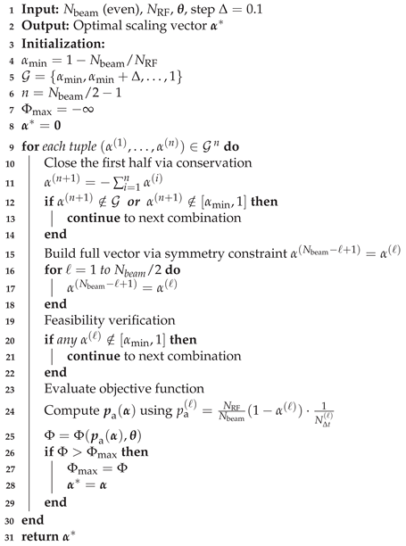 |
- 1.
- Exploit symmetry and conservation constraints to reduce the search space from to independent variables.
- 2.
- Enumerate all feasible combinations over a discrete grid for computational tractability.
- 3.
- For each independent variable combination, compute the dependent variable using conservation and reconstruct the full vector via symmetry.
- 4.
- Verify that all computed variables satisfy the bound constraints before evaluation.
- 5.
- Assess the objective function for all feasible configurations and select the optimal solution.
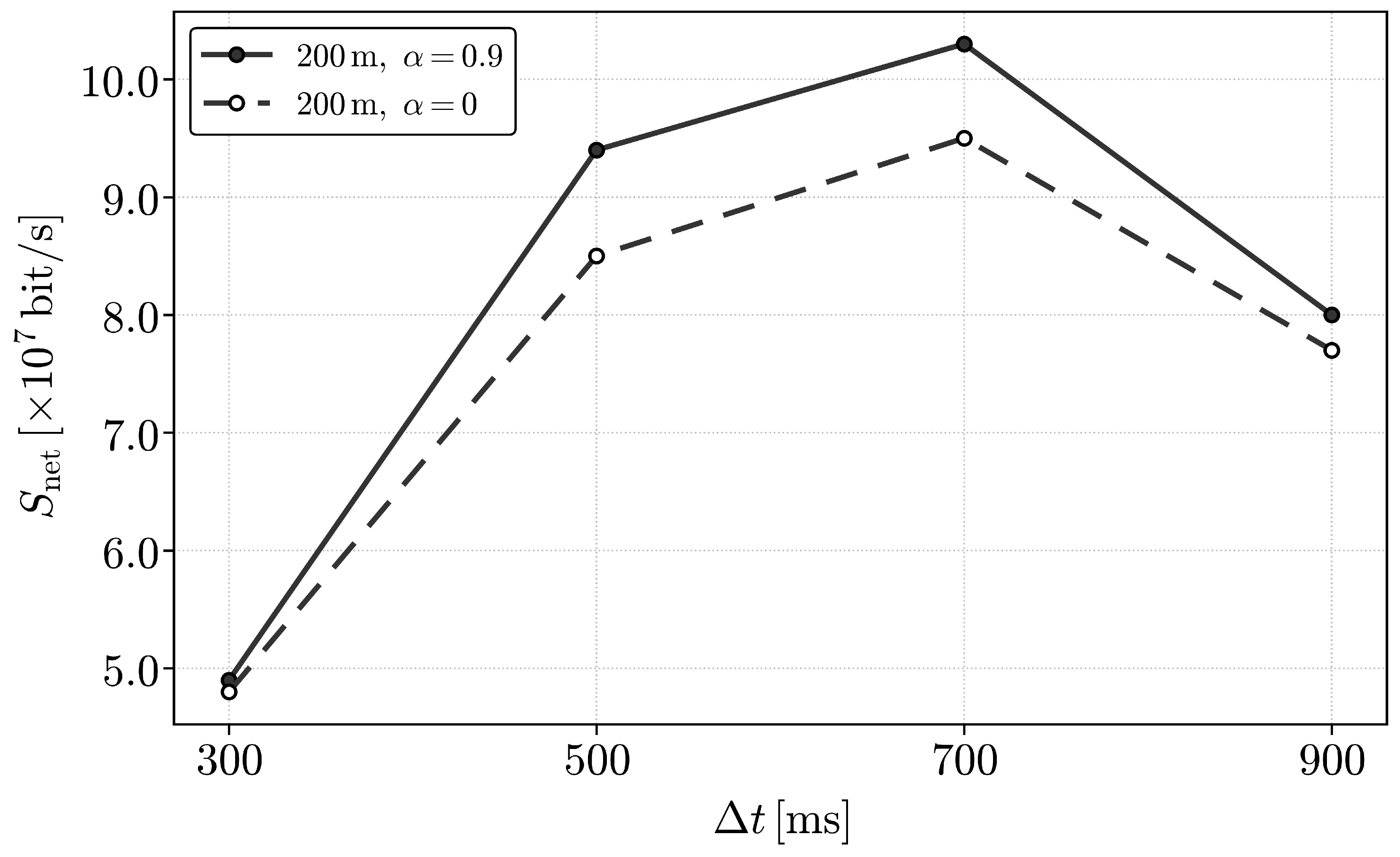
As an illustrative application of the proposed beam-activation optimization, Figure A1 reports the network throughput under periodic traffic for , varying , with and . In this setting, symmetry pairs the beams as and , so that and ; enforcing conservation yields leaving a single degree of freedom (). Using the parameters in Table 2, the optimal configuration is and . This shifts the activation pattern from the uniform baseline (, each beam active of the time) to a specialized scheme in which the central beams 2 and 3 are active about of the time, while the outer beams 1 and 4 operate about of the time. Compared with the uniform case, the optimized schedule yields up to a 12% throughput gain, attained at the where the gap between the two curves in Figure A1 is maximal.
Figure A1.
Network throughput under periodic traffic, as a function of the RRA interval duration , for fixed UAV altitudes h and .
Figure A1.
Network throughput under periodic traffic, as a function of the RRA interval duration , for fixed UAV altitudes h and .
References
- 6G Flagship. 6G Research Verticals, 2024. Accessed on 3 January 2026.
- Liu, J.; Peng, S.; Tong, X. Non-Terrestrial Networks in 6G on Standardization, Key Technologies and Challenges. In Proceedings of the 2025 International Wireless Communications and Mobile Computing (IWCMC), 2025, pp. 222–226. [CrossRef]
- Spampinato, L.; Ferretti, D.; Buratti, C.; Marini, R. Joint Trajectory Design and Radio Resource Management for UAV-Aided Vehicular Networks. IEEE Transactions on Vehicular Technology 2025, 74, 847–860. [CrossRef]
- Study on New Radio (NR) to Support Non-Terrestrial Networks (Release 15). 3GPP Technical Report TR 38.811 V15.4.0, 3rd Generation Partnership Project (3GPP), 2020. Available at: https://www.3gpp.org/ftp/Specs/archive/38_series/38.811/38811-f40.zip.
- Dong, K.; Mizmizi, M.; Tagliaferri, D.; Spagnolini, U. Vehicular Blockage Modelling and Performance Analysis for mmWave V2V Communications. In Proceedings of the ICC 2022 - IEEE International Conference on Communications, 2022, pp. 3604–3609. [CrossRef]
- Ma, X.; Su, Z.; Xu, Q.; Ying, B. Edge Computing and UAV Swarm Cooperative Task Offloading in Vehicular Networks. In Proceedings of the 2022 International Wireless Communications and Mobile Computing (IWCMC), 2022, pp. 955–960. [CrossRef]
- Xiao, T.; Du, P.; Gou, H.; Zhang, G. NOMA-MEC Based Task Offloading Algorithm in UAV-Assisted IoV Networks. In Proceedings of the 2024 3rd International Conference on Computing, Communication, Perception and Quantum Technology (CCPQT), 2024, pp. 190–194. [CrossRef]
- Wlodarczyk, D.; Saber, T. Assessing Potential of UAV-Based Increase in Urban Disasters Communication on Traffic Congestion Mitigation. In Proceedings of the 2024 International Conference on Information and Communication Technologies for Disaster Management (ICT-DM), 2024, pp. 1–7. [CrossRef]
- Fan, X.; Zhang, H.; Huang, Y.; Su, Y.; Li, H.; Huo, J.; Sun, C.; Hao, S.; Zhen, L. Temporal Data Dissemination in UAV-Assisted VANETs Through Time-Varying Graphs. IEEE Transactions on Vehicular Technology 2024, 73, 14835–14846. [CrossRef]
- Yuan, T.; Rothenberg, C.E.; Obraczka, K.; Barakat, C.; Turletti, T. Harnessing UAVs for Fair 5G Bandwidth Allocation in Vehicular Communication via Deep Reinforcement Learning. IEEE Transactions on Network and Service Management 2021, 18, 4063–4074. [CrossRef]
- Hosseini, M.; Ghazizadeh, R. Stackelberg Game-Based Deployment Design and Radio Resource Allocation in Coordinated UAVs-Assisted Vehicular Communication Networks. IEEE Transactions on Vehicular Technology 2023, 72, 1196–1210. [CrossRef]
- Conserva, F.; Verdone, R. Analytical Description of Access Probability and RRA Strategy for UAV-Aided Vehicular Applications. In Proceedings of the Proceedings of the Ninth Workshop on Micro Aerial Vehicle Networks, Systems, and Applications, New York, NY, USA, 2023; DroNet ’23, p. 21–26. [CrossRef]
- Li, J.; Niu, Y.; Wu, H.; Ai, B.; He, R.; Wang, N.; Chen, S. Joint Optimization of Relay Selection and Transmission Scheduling for UAV-Aided mmWave Vehicular Networks. IEEE Transactions on Vehicular Technology 2023, 72, 6322–6334. [CrossRef]
- Guhagarkar, A.; Sivalingam, T.; Bhatia, V.; Rajatheva, N.; Latva-Aho, M. Reinforcement Learning-Based Optimization of Relay Selection and Transmission Scheduling for UAV-Aided mmWave Vehicular Networks. In Proceedings of the 2024 27th International Symposium on Wireless Personal Multimedia Communications (WPMC), 2024, pp. 1–5. [CrossRef]
- Khan, N.; Ahmad, A.; Wakeel, A.; Kaleem, Z.; Rashid, B.; Khalid, W. Efficient UAVs Deployment and Resource Allocation in UAV-Relay Assisted Public Safety Networks for Video Transmission. IEEE Access 2024, 12, 4561–4574. [CrossRef]
- Liang, W.; Ma, S.; Yang, S.; Zhang, B.; Gao, A. Hierarchical Matching Algorithm for Relay Selection in MEC-Aided Ultra-Dense UAV Networks. Drones 2023, 7. [CrossRef]
- Chen, X.; Zhang, G.; Han, G.; Peng, Z. Resource Management with Blockchain for Delay-Sensitive Transmission in UAV-assisted Vehicular Network. In Proceedings of the 2024 4th International Conference on Neural Networks, Information and Communication Engineering (NNICE), 2024, pp. 506–510. [CrossRef]
- Ismail, M.; Muhammad, F.; Shafiq, Z.; Irfan, M.; Rahman, S.; Mursal, S.N.F.; Nowakowski, G.; Zharikov, E. Line-of-Sight-Based Coordinated Channel Resource Allocation Management in UAV-Assisted Vehicular Ad Hoc Networks. IEEE Access 2024, 12, 25245–25253. [CrossRef]
- Gai, H.; Zhang, H.; Guo, S.; Yuan, D. Information Freshness-Oriented Trajectory Planning and Resource Allocation for UAV-assisted Vehicular Networks. China Communications 2023, 20, 244–262. [CrossRef]
- Conserva, F.; Linsalata, F.; Mizmizi, M.; Magarini, M.; Spagnolini, U.; Verdone, R.; Buratti, C. A Thorough Analysis of Radio Resource Assignment for UAV-Enhanced Vehicular Sidelink Communications. In Proceedings of the ICC 2024 - IEEE International Conference on Communications, 2024, pp. 4341–4346. [CrossRef]
- Chen, L.; Du, J.; Zhu, X. Mobility-Aware Task Offloading and Resource Allocation in UAV-Assisted Vehicular Edge Computing Networks. Drones 2024, 8. [CrossRef]
- Li, S.; Yoshii, K.; Shimamoto, S.; Ho, T.D. Optimizing mmWave UAV Networks: Mobility-Aware Deployment and Resource Allocation. In Proceedings of the 2024 IEEE 100th Vehicular Technology Conference (VTC2024-Fall), 2024, pp. 1–5. [CrossRef]
- Peer, M.; Bohara, V.A.; Srivastava, A.; Ghatak, G. User Mobility-Aware UAV-BS Placement Update With Optimal Resource Allocation. IEEE Open Journal of the Communications Society 2022, 3, 1853–1866. [CrossRef]
- Orikumhi, I.; Bae, J.; Kim, S. Mobility-Aware Resource Allocation in UAV-Assisted ISAC Networks. In Proceedings of the 2023 14th International Conference on Information and Communication Technology Convergence (ICTC), 2023, pp. 1042–1044. [CrossRef]
- Hoang, L.T.; Nguyen, C.T.; Li, P.; Pham, A.T. Joint Uplink and Downlink Resource Allocation for UAV-enabled MEC Networks under User Mobility. In Proceedings of the 2022 IEEE International Conference on Communications Workshops (ICC Workshops), 2022, pp. 1059–1064. [CrossRef]
- Wang, J.; Zhang, H.; Zhou, X.; Yuan, D. UAV-Assisted Wireless Networks: Mobility and Service Oriented Power Allocation and Trajectory Design. IEEE Transactions on Vehicular Technology 2024, 73, 17373–17383. [CrossRef]
- ETSI EN 302 637-2 V1.3.2. Intelligent Transport Systems (ITS); Vehicular Communications; Basic Set of Applications; Part 2: Specification of Cooperative Awareness Basic Service, 2014.
- 3GPP. Enhancement of 3GPP Support for V2X Scenarios; Stage 1 (Release 18). TS 22.186 V18.0.1, 2024.
- Mignardi, S.; Ferretti, D.; Marini, R.; Conserva, F.; Bartoletti, S.; Verdone, R.; Buratti, C. Optimizing Beam Selection and Resource Allocation in UAV-Aided Vehicular Networks. In Proceedings of the 2022 Joint European Conference on Networks and Communications & 6G Summit (EuCNC/6G Summit), 2022, pp. 184–189. [CrossRef]
- Yang, D.; Yang, L.L.; Hanzo, L. DFT-Based Beamforming Weight-Vector Codebook Design for Spatially Correlated Channels in the Unitary Precoding Aided Multiuser Downlink. In Proceedings of the 2010 IEEE International Conference on Communications, 2010, pp. 1–5. [CrossRef]
- Shakhatreh, H.; Malkawi, W.; Sawalmeh, A.; Almutiry, M.; Alenezi, A. Modeling Ground-to-Air Path Loss for Millimeter Wave UAV Networks, 2021, [arXiv:cs.IT/2101.12024].
- 3GPP. NR; NR and NG-RAN Overall Description; Stage 2 (Release 18). TS 38.300 V18.4.0, 2024.
- Morandi, F.; Linsalata, F.; Brambilla, M.; Mizmizi, M.; Magarini, M.; Spagnolini, U. A Probabilistic Codebook Technique for Fast Initial Access in 6G Vehicle-to-Vehicle Communications. In Proceedings of the 2021 IEEE International Conference on Communications Workshops (ICC Workshops), 2021, pp. 1–6. [CrossRef]
- Haykin, S. Communication Systems; John Wiley & Sons, 2000.
- Dahlman, E.; Parkvall, S.; Skold, J. 5G NR: The Next Generation Wireless Access Technology, 1st ed.; Academic Press, Inc.: USA, 2018.
- Dong, K.; Mizmizi, M.; Tagliaferri, D.; Spagnolini, U. Vehicular Blockage Modelling and Performance Analysis for mmWave V2V Communications. In Proceedings of the ICC 2022 - IEEE International Conference on Communications, 2022, pp. 3604–3609. [CrossRef]
- Bartoletti, S.; Masini, B.M.; Martinez, V.; Sarris, I.; Bazzi, A. Impact of the Generation Interval on the Performance of Sidelink C-V2X Autonomous Mode. IEEE Access 2021, 9, 35121–35135. [CrossRef]
- ETSI. Intelligent Transport Systems (ITS); Vehicular Communications; Basic Set of Applications; Part 2: Specification of Cooperative Awareness Basic Service. Technical Report ETSI EN 302 637-2 V1.4.1, ETSI, 2019. Published April 2019.
- Linsalata, F.; Mura, S.; Mizmizi, M.; Magarini, M.; Wang, P.; Khormuji, M.N.; Perotti, A.; Spagnolini, U. LoS-Map Construction for Proactive Relay of Opportunity Selection in 6G V2X Systems. IEEE Transactions on Vehicular Technology 2023, 72, 3864–3878. [CrossRef]
- Kleinrock, L. Queueing Systems, Vol. I: Theory; Wiley, New York, 1975.
- Peyhardi, J. On Quasi Polya Thinning Operator. Brazilian Journal of Probability and Statistics 2023. In press, . [CrossRef]
- Mizmizi, M.; Tagliaferri, D.; Badini, D.; Mazzucco, C.; Spagnolini, U. Channel Estimation for 6G V2X Hybrid Systems Using Multi-Vehicular Learning. IEEE Access 2021, 9, 95775–95790. [CrossRef]
Short Biography of Authors
 |
Francesca Conserva received the B.Sc. and M.Sc. degrees in Telecommunications Engineering and the Ph.D. degree in Electronics, Telecommunications, and Information Technologies Engineering from the University of Bologna. Her doctoral research focused on the design of mobility-aware radio resource management algorithms for UAV-aided vehicular networks and on AI-based predictive frameworks for RAN optimization using network KPIs in beyond-5G networks. She is currently a Researcher at WiLab (CNIT), where her research interests include Network Digital Twin technologies, UAV-assisted networks, and AI-driven RAN optimization. |
 |
Chiara Buratti received the Ph.D. degree in Electronics, Information Technologies, and Telecommunications Engineering from the University of Bologna, Bologna, Italy, in 2009. She is currently an Associate Professor with the University of Bologna. She has coauthored approximately 120 scientific papers. Her research interests include the Internet of Things, with emphasis on MAC and routing protocols, and three-dimensional networks. She was the recipient of the 2012 Intel Early Career Faculty Honor Program Award and the 2010 National GTTI Best Ph.D. Thesis Award. She was the main proponent of the COST Action CA20120 (INTERACT) and is currently its Vice-Chair and Grant Holder. |
| 1 | A unit-size queue is assumed; a new packet is generated only when the queue is empty. |
Figure 1.
UAV-aided V2V communication scenario featuring two UAVs () serving the road segment from point A to point B. Each UAV is equipped with four beams () and three Radio Frequency (RF) chains ().
Figure 1.
UAV-aided V2V communication scenario featuring two UAVs () serving the road segment from point A to point B. Each UAV is equipped with four beams () and three Radio Frequency (RF) chains ().
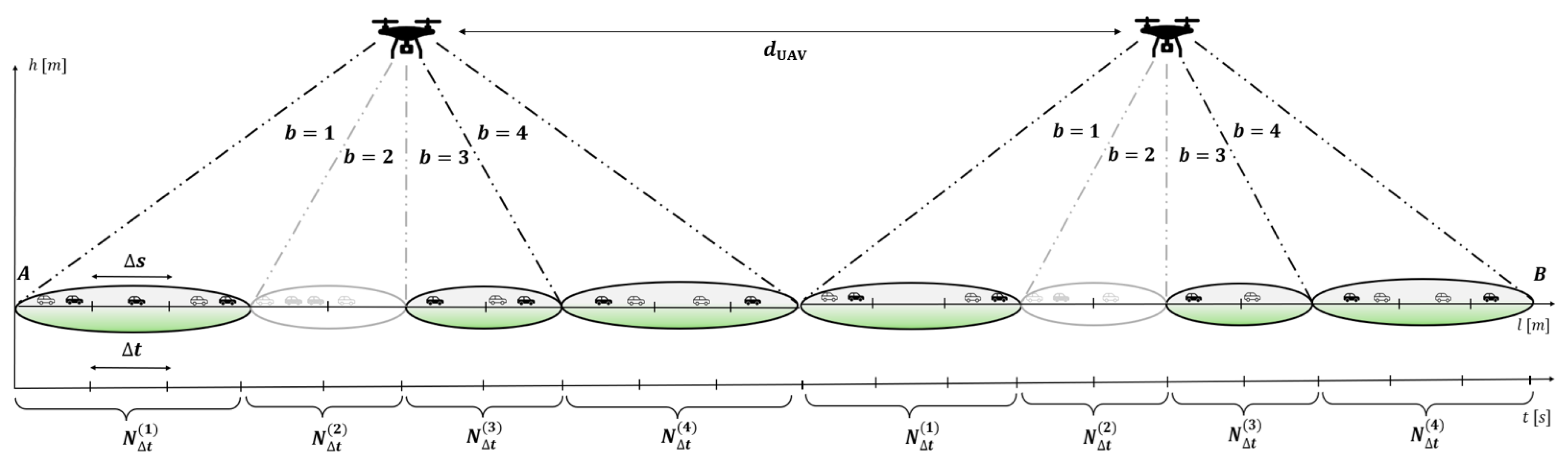
Figure 2.
Example of TDMA scheme applied to active beams out of beams.
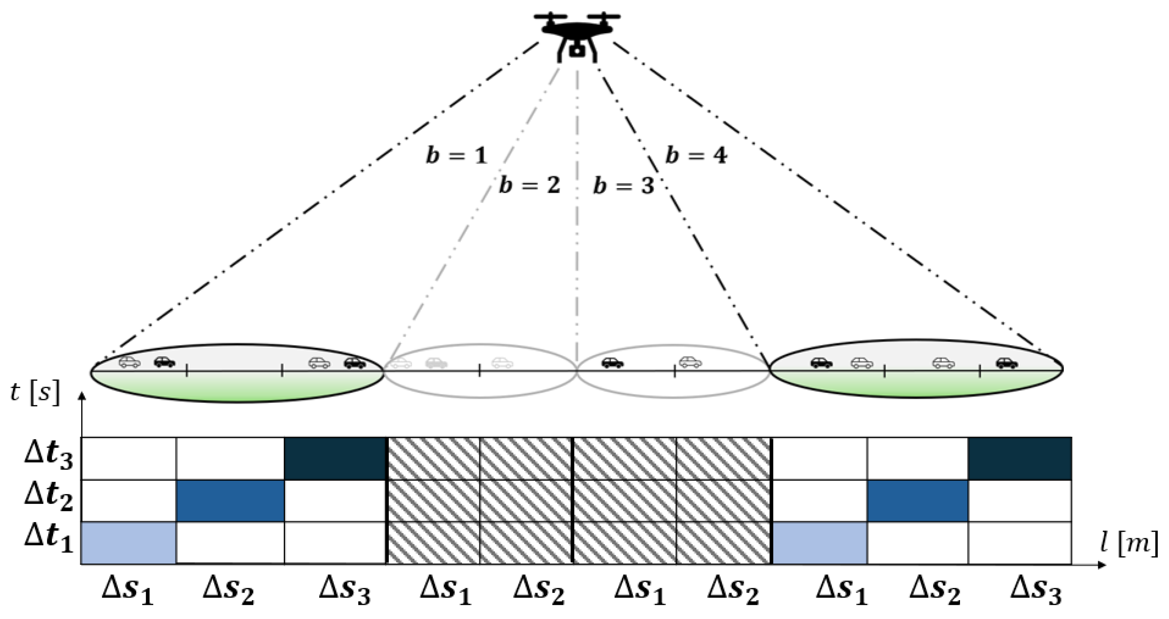
Figure 3.
CAV’s average success probability under periodic traffic, as a function of the RRA interval duration , for different UAV altitudes h.
Figure 3.
CAV’s average success probability under periodic traffic, as a function of the RRA interval duration , for different UAV altitudes h.
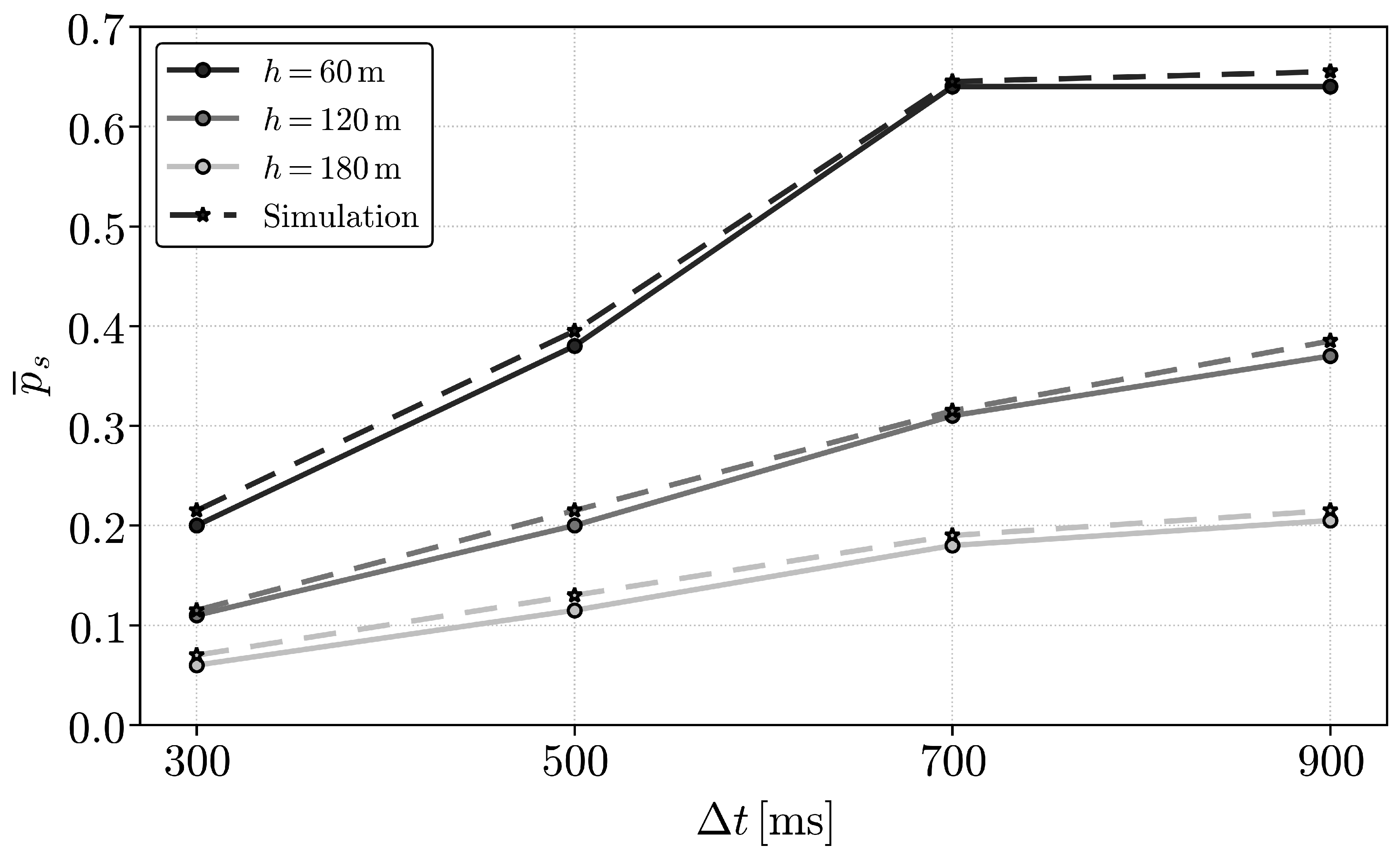
Figure 4.
CAV’s average throughput under periodic traffic, as a function of the RRA interval duration , for different UAV altitudes h.
Figure 4.
CAV’s average throughput under periodic traffic, as a function of the RRA interval duration , for different UAV altitudes h.
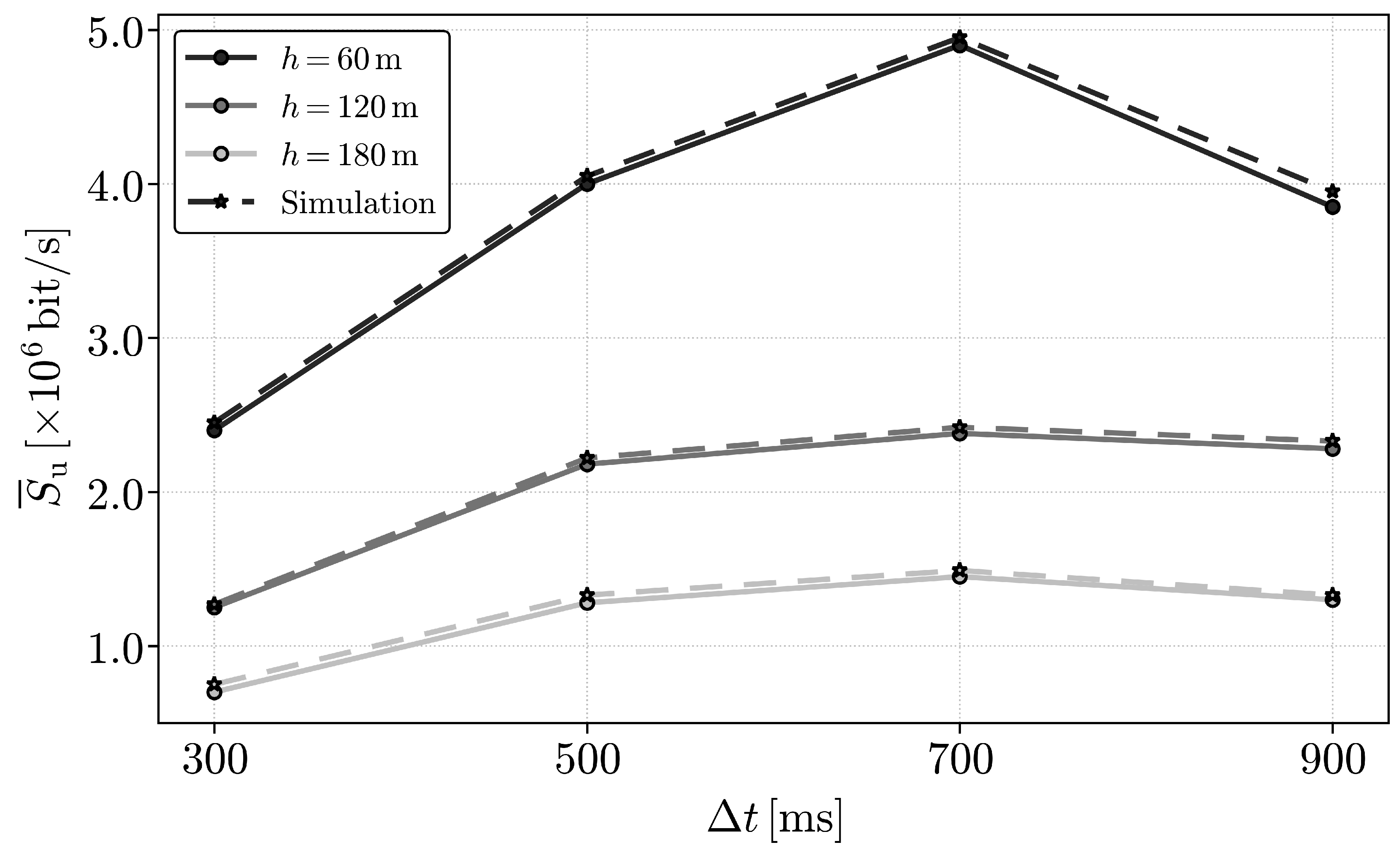
Figure 5.
CAV’s average throughput under periodic and probabilistic traffic models, as a function of the total generated traffic in bits, G, for varying RRA interval durations and UAV altitudes h.
Figure 5.
CAV’s average throughput under periodic and probabilistic traffic models, as a function of the total generated traffic in bits, G, for varying RRA interval durations and UAV altitudes h.
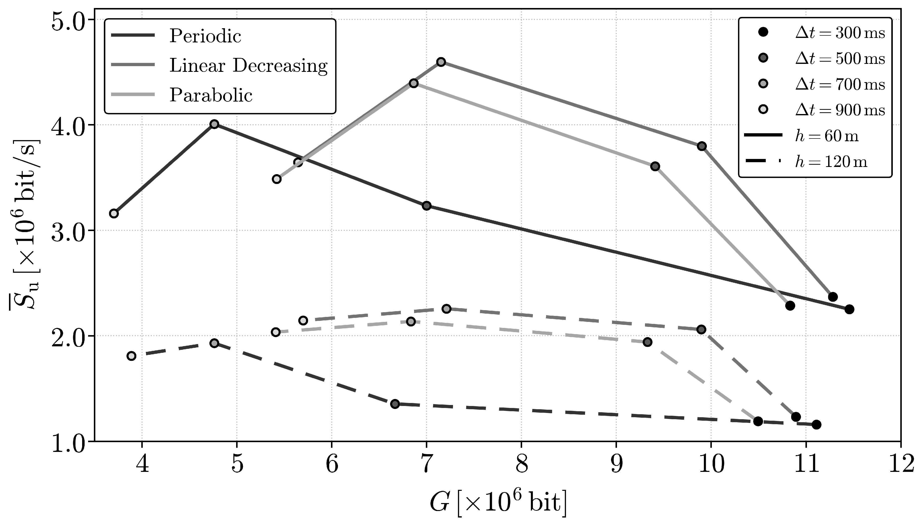
Table 2.
Input parameters.
| Parameter | Notation | Value |
|---|---|---|
| Number of UAVs | 2 | |
| CAV’s antenna elements | 4 | |
| UAV’s antenna elements | 5 | |
| CAV’s transmitting power | 23 dBm | |
| CAV’s speed | v | 33.3 m/s |
| Vehicle’s average length | 5 m | |
| Noise power | -101 dBm | |
| Excess path loss offset | A | 84.64 dB |
| Path loss exponent | 1.55 | |
| Log-normal shadowing variance | 4 | |
| Vehicle density | 80 cars/km | |
| SNR threshold | 13 dB | |
| Carrier frequency | 28 GHz | |
| Bandwidth available per beam | B | 30 MHz |
| PRBs per channel | 10 | |
| Subcarriers per channel | 12 | |
| Subcarrier spacing | 120 KHz | |
| Demand | D | 10 Mbit |
| Slot duration | 125 s | |
| Max. packet generation probability | 0.9 | |
| Min. packet generation probability | 0.6 |
Disclaimer/Publisher’s Note: The statements, opinions and data contained in all publications are solely those of the individual author(s) and contributor(s) and not of MDPI and/or the editor(s). MDPI and/or the editor(s) disclaim responsibility for any injury to people or property resulting from any ideas, methods, instructions or products referred to in the content. |
© 2026 by the authors. Licensee MDPI, Basel, Switzerland. This article is an open access article distributed under the terms and conditions of the Creative Commons Attribution (CC BY) license (http://creativecommons.org/licenses/by/4.0/).
Copyright: This open access article is published under a Creative Commons CC BY 4.0 license, which permit the free download, distribution, and reuse, provided that the author and preprint are cited in any reuse.


