Submitted:
11 January 2026
Posted:
13 January 2026
You are already at the latest version
Abstract
Electric-vehicle (EV) diffusion exhibits nonlinear, path-dependent dynamics shaped by interacting economic, technological, and social constraints. This paper develops a unified hybrid-systems framework that captures these complexities by integrating microfounded household choice, capacity constrained firm behavior, local network spillovers, and multi-level policy intervention within a Filippov differential-inclusion structure. Households face heterogeneous preferences, liquidity limits, and network-mediated moral and informational influences; firms invest irreversibly under learning-by-doing and profitability thresholds; and national and local governments implement distinct financial and infrastructure policies subject to budget constraints. The resulting aggregate adoption dynamics feature endogenous switching, sliding modes at economic bottlenecks, network-amplified tipping, and hysteresis arising from irreversible investment. We establish conditions for the existence of Filippov solutions, derive network-dependent tipping thresholds, characterize sliding regimes at capacity and liquidity constraints, and show how network structure magnifies hysteresis and shapes the effectiveness of local versus national policy. Optimal-control analysis further demonstrates that national subsidies follow bang--bang patterns and that network-targeted local interventions minimize the fiscal cost of achieving regional tipping. The framework provides a complex-systems perspective on sustainable mobility transitions and clarifies why identical national policies can generate asynchronous regional outcomes. These results offer theoretical foundations for designing coordinated, cost-effective, and network-aware EV transition strategies.
Keywords:
complex adaptive systems
; hybrid dynamical systems
; non-smooth dynamics
; network-driven diffusion
; tipping points
; electric vehicle adoption
1. Introduction
The transition from internal combustion engine (ICE) vehicles to electric vehicles (EVs) is widely regarded as a central component of contemporary sustainable mobility transitions. Electrification is expected to mitigate climate change, improve urban air quality, and reduce public-health outcomes, yet its aggregate effects are neither automatic nor uniform. Life-cycle assessments show that the environmental performance of EVs depends critically on electricity generation mixes and usage conditions [1], while broader reviews emphasize technological, organizational, and policy co-benefits that accompany large-scale adoption [2]. Macro-level evidence further indicates that EV diffusion can reduce transport-sector CO2 emissions, although realized outcomes depend strongly on policy design and institutional context [3]. These findings suggest that electrification is best understood not as a smooth technological substitution, but as a socio-technical transition emerging from the interaction of multiple interdependent subsystems.
From a complex-systems perspective, EV adoption exhibits the defining characteristics of a complex adaptive system: heterogeneous agents, nonlinear feedbacks, network externalities, hard constraints, and the coexistence of multiple macroscopic regimes. In such systems, aggregate behavior emerges endogenously from structured interactions rather than from representative or average responses, and small perturbations in incentives or constraints can trigger disproportionate and discontinuous system-wide responses [4]. These features imply that path dependence, tipping points, and hysteresis are not anomalies but structural properties of the adoption process.
Empirical adoption studies confirm this interpretation. Cross-national and city-level analyses show that financial incentives, charging infrastructure, and socio-demographic factors influence EV uptake, but that no single determinant reliably induces sustained diffusion [5,6,7,8]. Behavioral and discrete-choice models further demonstrate that adoption unfolds through distinct stages and is strongly shaped by social reinforcement mechanisms [9,10]. Network-oriented studies reveal nonlinear stock effects of charging infrastructure and strong interactions between peer influence and policy timing, indicating the presence of threshold-driven and cascade-like diffusion dynamics [11,12]. Together, this literature points to an intrinsically path-dependent adoption process in which local interactions can produce abrupt aggregate transitions.
At more aggregate levels, system-dynamics and simulation-based models highlight long-run feedbacks linking EV uptake to energy systems, health outcomes, and public expenditures [13,14,15]. Innovation-system approaches similarly emphasize the co-evolution of technology, acceptance, and policy during mobility transitions [16]. However, most existing models impose smooth adjustment or exogenous regime changes, limiting their ability to represent endogenous switching between adoption regimes. Insights from network science and statistical physics indicate that systems with thresholds and interdependencies can undergo abrupt hybrid phase transitions characterized by cascades, avalanches, and regime persistence [17,18]. From a systems-theoretic perspective, persistence in such settings is better described by homeodynamics—transitions among alternative stable states—than by convergence to a single equilibrium [19].
Recent advances in hybrid and non-smooth dynamical systems provide a natural formal framework for capturing these features. By explicitly modeling switching surfaces, binding constraints, and regime-dependent dynamics, hybrid systems theory allows discontinuities and constraint activation to be treated as structural components of system evolution rather than as modeling artifacts [20]. Despite their relevance, such approaches remain largely underutilized in economic models of technology adoption.
This paper addresses this gap by developing a unified hybrid-system model of EV adoption, formulated as a Filippov differential inclusion. The central research question is: under what conditions do interacting household behavior, firm dynamics, infrastructure constraints, and policy instruments generate tipping points, stagnation traps, or irreversible adoption regimes? The model integrates micro-level adoption decisions, meso-level industry dynamics, and macro-level constraints within a single non-smooth dynamical framework, allowing regime switching, hysteresis, and policy-induced discontinuities to emerge endogenously from the system’s internal structure rather than being imposed exogenously.
The remainder of the paper is organized as follows. Section 2 develops the economic microfoundations of the adoption system. Section 3 reformulates the resulting dynamics as a hybrid system using a Filippov differential inclusion. Section 5 presents the analytical and numerical results. Section 6 discusses implications for adoption dynamics and transition policy. Section 7 concludes.
2. Economic Microfoundations of a Complex Adoption System
Electric vehicle diffusion arises from the interaction of heterogeneous households, profit-maximizing firms, and public authorities operating under technological, fiscal, and infrastructural constraints. These interactions unfold on social and market networks, propagate through prices and investment decisions, and feed back into policy and capacity regimes. As a result, EV adoption exhibits hallmark features of complex adaptive systems: nonlinear amplification, threshold effects, path dependence, and the coexistence of multiple adoption regimes rather than smooth, equilibrium adjustment.
This section develops a fully microfounded economic model that makes these complexity features explicit. Individual optimization under heterogeneous constraints generates network spillovers and endogenous feedbacks at the meso level of firms, infrastructure provision, and industry capacity. These meso-level dynamics, in turn, reshape the macroeconomic environment by activating or relaxing binding constraints, thereby inducing regime switching in aggregate adoption. The model therefore links micro-level decision-making, meso-level market and network structure, and macro-level policy and capacity limits within a dynamically coupled system, setting the stage for the hybrid and non-smooth dynamics formalized later through Filippov differential inclusions.
2.1. Population, Regions, and Networks
Time is continuous, . The economy consists of a finite population of consumers indexed by , where . Consumers are embedded in a social interaction network
where denotes the set of social links. An edge represents a persistent social, informational, or observational relationship between consumers i and j. These links capture peer interaction, neighborhood visibility, workplace communication, family ties, and online social exposure through which consumers exchange information, form expectations, and update social norms regarding electric vehicle (EV) adoption. The network therefore constitutes the primary channel through which confidence in EV technology, perceived feasibility, reputational benefits, and moral valuation propagate endogenously through the population.
Each ordered pair is associated with a nonnegative weight measuring the intensity of social influence from agent j to agent i. The corresponding weighted adjacency (influence) matrix is denoted by
where if and only if , and otherwise. The network is assumed to be static over time and nonnegative. We impose the uniform boundedness condition
for some finite constant , which ensures that aggregate peer influence on any individual is uniformly bounded.
We further assume that each regional influence matrix induced by the subnetwork on is nonnegative and irreducible. Let denote the Perron–Frobenius eigenvalue (spectral radius) of W. Under these assumptions, is well defined and associated with a strictly positive eigenvector. Throughout the analysis, serves as a reduced-form measure of network connectivity and influence intensity. Differences in capture variation in the strength of social spillovers across regions and directly enter the tipping, hysteresis, and targeted-policy results derived later in the paper.
Consumers are geographically distributed across a finite set of regions ,
Regional partitioning captures spatial heterogeneity in charging infrastructure, electricity and fuel prices, income distributions, travel patterns, and local policy environments. Social interactions may extend across regions through the global network W, but market prices, infrastructure constraints, and policy instruments are region-specific.
Preference heterogeneity operates at the individual level. Each consumer belongs to one of two preference classes,
where ethical consumers internalize environmental externalities, reputational payoffs, and social norms associated with EV adoption, while standard consumers respond only to private economic costs and benefits. This heterogeneity generates asymmetric network responses: identical price signals and subsidies can trigger strong local cascades in socially responsive groups while leaving others largely unaffected.
At each instant t, consumers observe regional market prices and the current vector of national and regional policy instruments,
However, perceptions of EV reliability, operating costs, and social desirability evolve endogenously through network exposure rather than being instantaneously or uniformly known. As a result, price and policy signals are translated into adoption behavior through a socially mediated learning and coordination process rather than through purely individual optimization.
2.2. Household Optimization and Discrete Choice
At each instant t, consumer i selects one durable technology . Let denote income, and the region-r market-clearing prices of EVs and ICE vehicles, the per-unit EV subsidy faced by consumers in region r, and non-durable consumption. We interpret vehicle prices as equivalent flow (user-cost) representations of durable adoption. The net purchase price of an EV is . Consumers face the budget and liquidity constraints
If , EV adoption is infeasible regardless of preferences, generating corner solutions that will later induce non-smooth aggregate dynamics. Consumers maximize discounted lifetime utility with discount rate and instantaneous utility . We assume that , , and are bounded or of at most exponential growth, ensuring that the discounted utility integrals below are well defined.
For ethical consumers,
where and denote region-specific operating costs and captures the weight placed on moral and reputational benefits. Standard consumers set . Unobserved preference heterogeneity enters through i.i.d. Type-I extreme-value shocks , so that indirect utility is . The resulting EV adoption probability is therefore given by the multinomial logit rule
subject to the feasibility condition .
Social diffusion of moral valuation
Moral and reputational benefits evolve endogenously through social interaction. Let denote consumer i’s moral valuation of EV adoption. We assume follows a network diffusion process,
where measures the strength of social reinforcement and is the decay rate. Under the boundedness assumption on W, (11) admits a unique absolutely continuous solution for any initial condition , and remains uniformly bounded over time. The region-level moral valuation entering household utility is defined as the within-region average
This formulation ensures that moral valuation is microfounded at the individual level while allowing social reinforcement to aggregate into a region-specific ethical externality.
2.3. Firms, Capacity, and Investment
The supply side consists of a set of firms , where are EV specialists and are multi-product firms producing both EVs and ICE vehicles. All firms face short-run capacity constraints,
which may bind when demand increases rapidly or when capacity expansion lags behind market growth. EV production exhibits learning-by-doing: cumulative output lowers marginal cost according to
capturing well-established battery- and assembly-learning effects. This generates path dependence: early production accelerates later cost reductions. Given regional market prices, EV specialists choose output by solving
while multi-product firms allocate production across technologies,
internalizing both EV learning and potential EV–ICE cannibalization effects. Capacity evolves through irreversible investment,
where firms expand capacity only when current profits exceed a minimum threshold,
This threshold rule generates endogenous regime switching. Modest shifts in profitability driven by demand growth, policy changes, or learning effects can induce discrete changes in investment activity. Negative shocks, by contrast, may abruptly arrest expansion and create persistent supply bottlenecks. Learning, capacity constraints, and threshold-based investment decisions therefore act as a central nonlinear mechanism linking firm behavior to aggregate EV diffusion.
2.4. Market Clearing and Aggregate Adoption
Regional markets link decentralized household decisions and firm-level production to equilibrium prices and aggregate adoption. Total EV supply in region r is the sum of firm outputs,
and market clearing requires that EV sales equal realized demand,
ensuring that inventories or backlogs do not accumulate in equilibrium. The market-clearing price adjusts to balance heterogeneous household willingness-to-pay with available firm capacity, learning-driven cost reductions, and regional policies. We represent this price as an implicit function of the regional economic state,
where denotes the local adoption rate, aggregate productive capacity, local subsidies or taxes, and regional social influence or information conditions. This formulation captures essential nonlinearities. Changes in adoption levels, infrastructure availability, or policy parameters can induce discontinuous price responses when firms face binding capacity constraints or experience learning-driven cost reductions.
Aggregate adoption in region r evolves from individual choices on the household network,
providing the macro-level state variable that feeds back into prices, network spillovers, and firm profitability. Thus, market clearing closes the micro–meso–macro loop: household adoption affects prices, prices influence firm output and investment, and changing supply conditions feed back into adoption dynamics.
3. Non-Smooth Regime Dynamics in a Complex Adoption System
The equilibrium dynamics of EV adoption are intrinsically non-smooth, arising from the interaction of microeconomic, infrastructural, and policy constraints. Household demand becomes liquidity constrained as EV prices approach income limits. Firms endogenously switch between unconstrained and capacity-saturated production regimes. Charging infrastructure exhibits congestion once network thresholds are reached, while public budgets trigger abrupt subsidy withdrawal when fiscal limits bind. These interacting constraints generate discontinuities in best responses, prices, and investment decisions, precluding a smooth dynamical description.
Aggregate adoption is therefore naturally represented by a Filippov differential inclusion [21], in which the governing vector field changes across endogenously generated switching surfaces. This formulation captures regime transitions, sliding dynamics, and abrupt constraint-induced adjustments as intrinsic features of the adoption process rather than as exogenous shocks (Recent work by Stiefenhofer develops a geometric and contraction-based framework for Filippov systems in higher-dimensional and complex-valued state spaces, with particular emphasis on the existence and stability of nonsmooth periodic orbits [22,23,24]).
Let the reduced-form regional adoption dynamics be
where denotes the market-clearing EV price, regional subsidies or taxes, aggregate production capacity, the remaining subsidy budget, and effective charging infrastructure. Each state variable evolves according to a piecewise-smooth law: prices change slope when capacity binds, subsidies jump when budgets are exhausted, capacity adjusts discretely once profitability exceeds an investment threshold, and infrastructure switches between uncongested and congested regimes.
Let denote the union of all switching surfaces associated with occasionally binding constraints in region r, including subsidy exhaustion, capacity saturation, household liquidity limits, infrastructure congestion, and investment triggers. Across these surfaces, the macroeconomic vector field governing adoption takes the Filippov form
where and correspond to distinct economic regimes and denotes the convex hull defining sliding dynamics along regime boundaries.
This hybrid formulation captures subsidy cutoffs, investment thresholds, congestion onset, and liquidity-binding transitions within a unified dynamical system. The resulting adoption economy is a non-smooth, path-dependent complex system whose trajectories may exhibit sliding motions, boundary equilibria, hysteresis, and abrupt regime shifts. In this sense, aggregate EV diffusion emerges from the interaction of heterogeneous agents, networks, and constraints across scales, with qualitative system behavior governed by regime structure rather than smooth adjustment.
4. Optimal Government Policy and Hybrid Economic Control
National and regional governments influence the EV transition through financial incentives and infrastructure provision. Let denote the per-unit EV subsidy in region r and public investment in charging infrastructure. Both instruments are subject to a regional fiscal budget evolving according to
where denotes exogenous revenues or intergovernmental transfers. Budget exhaustion () defines a binding constraint and an endogenous switching surface that can force abrupt policy adjustment.
Charging infrastructure evolves as a depreciating public capital stock,
directly affecting congestion, adoption thresholds, and the set of active regimes in the Filippov adoption dynamics. The government maximizes discounted regional welfare,
subject to the hybrid adoption dynamics and state constraints described above. Here captures societal benefits from EV adoption, including environmental, health, and network externalities, while denotes the marginal cost of infrastructure investment.
Because the Hamiltonian is linear in the control variables, optimal policy generically takes a bang–bang form,
implying discrete switches between high-support and zero-support regimes. These policy-induced discontinuities introduce additional switching surfaces that interact with those generated by liquidity constraints, production capacity limits, and infrastructure congestion.
The resulting policymaker–market interaction constitutes a hybrid optimal-control system. Policy interventions can trigger regime changes in adoption dynamics, while evolving market conditions endogenously activate or deactivate policy instruments. This bidirectional feedback generates tipping points, sliding regimes, and path-dependent transition trajectories that are central to the dynamics of EV diffusion. iu
5. Analysis and Results
This section examines the dynamic, network, and policy properties of the hybrid economic system developed in Sections 2–4. We highlight six central results: (i) network-dependent tipping, (ii) Filippov well-posedness, (iii) sliding regimes at economic bottlenecks, (iv) network-amplified hysteresis, (v) bang–bang optimal subsidies, and (vi) network-targeted policy efficiency. Throughout, we focus on a representative region r for notational simplicity and distinguish between national policies (shifting industry-wide prices and learning) and local policies (affecting infrastructure, operating costs, and network activation).
5.1. Network-Dependent Tipping of EV Adoption
We establish a network-dependent tipping threshold under the following structural assumptions on the reduced-form adoption dynamics.
Assumption A1
(Mean-field adoption dynamics). In region r, aggregate adoption follows the scalar ODE
where is continuously differentiable in and is the only network parameter entering .
Assumption A2
(Boundary conditions). For all admissible parameters,
so that and are always equilibria of (29).
Assumption A3
(Bistability). For the parameter region of interest, the equilibrium equation
admits three distinct solutions on , denoted , with stability signs
Assumption A4
(Network amplification). Peer effects raise net adoption incentives:
Theorem 1
(Network-Dependent Tipping Threshold). Let denote the largest eigenvalue of the regional influence matrix. Under Assumptions A1–A4, there exists a critical threshold
such that the long-run adoption outcome satisfies
where denote the low- and high-adoption equilibria. Moreover, the threshold is strictly decreasing in network connectivity:
Proof.
We proceed in three steps, invoking Assumptions A1–A4.
Step 1: Existence of an interior unstable equilibrium and definition of . By Assumption A1, aggregate adoption follows the one-dimensional ODE (29), with right-hand side continuously differentiable in x. By Assumption A2, the boundary points and are always equilibria of (29), as they satisfy (30). Assumption A3 states that, for the parameter region of interest, the equilibrium equation (31) admits three distinct solutions on , denoted
and that the local stability signs (32) hold at these equilibria. Since (29) is a scalar ODE with a right-hand side, it generates unique trajectories for every initial condition , and trajectories cannot cross. We define the tipping threshold as the interior unstable equilibrium:
By construction, depends on the parameters , as indicated in (34).
Step 2: Asymptotic convergence and threshold property. Consider the phase line on with equilibria . By continuity of in x (Assumption A1), and the fact that (31) has exactly these three simple roots on (Assumption A3), the sign of is constant on each open interval between equilibria. The derivative signs in (32) imply alternating sign changes across the roots. At the lower stable root , the derivative switches from positive to negative, indicating local stability. At the intermediate root , the sign reverses from negative to positive, identifying an unstable equilibrium. At the upper stable root , the derivative again changes from positive to negative, confirming stability at high adoption levels. Hence
and
Equations (38)–(39) together give the bistable sign pattern:
Now consider any initial condition . If , then by (40) we have as long as , so is strictly decreasing and bounded below by . By monotonicity and boundedness, has a limit as . If , this contradicts the fact that for all t; if , then continuity of and (40) imply , so remains negative near L, contradicting convergence. Thus the only possible limit is , so
Similarly, if , then (40) implies as long as , so is strictly increasing and bounded above by . By the same monotonicity argument, the limit as exists and must equal , so
Equations (41)–(42) together yield the asymptotic behavior stated in (35).
Step 3: Comparative statics with respect to . By definition of equilibrium, the tipping threshold satisfies
Equation (43) implicitly defines as a function of and the other parameters. Since is continuously differentiable (Assumption A1) and the derivative with respect to x at is strictly positive by (32), the implicit function theorem applies to (43). Differentiating (43) with respect to yields
Assumption A4 states that the numerator in (44) is strictly positive for , in particular at . Assumption A3 states that the denominator in (44) is strictly positive at the unstable equilibrium . Hence the fraction in (44) is strictly positive, and the leading minus sign implies
which is exactly the comparative-statics statement in (36). Equations (34), (35), and (36) follow directly from the construction in (37), the convergence analysis based on (40), and the implicit differentiation in (44)–(45), under Assumptions A1–A4. This completes the proof. □
Theorem 1 formalizes a mechanism consistent with empirical findings that social structure and network spillovers significantly shape EV diffusion. A higher spectral radius strengthens peer, informational, and moral spillovers, thereby reducing the critical mass required for self-sustaining adoption. This theoretical result mirrors evidence from municipal-level studies showing that denser charging or social networks accelerate diffusion through indirect or direct network effects [11,12,25]. Because also depends on regional operating costs and infrastructure capacity , local policies shift the tipping threshold directly, whereas national subsidy or carbon-pricing trajectories influence whether and when the system crosses it. Thus, tipping points in EV transitions arise endogenously from the interaction of network topology, regional conditions, and national policy environments.
5.2. Existence of Hybrid Filippov Dynamics
Theorem 2
(Filippov Well-Posedness). The equilibrium adoption dynamics
admit at least one absolutely continuous Filippov solution for every initial condition . Moreover, the interval is forward invariant: any solution starting in remains in for all .
Proof.
We consider the scalar differential inclusion (46) with state space and Filippov set-valued map defined as in Section 3. The proof proceeds in two steps: (i) existence of a Filippov solution, and (ii) forward invariance of .
Step 1: Existence of a Filippov solution. Recall that the hybrid adoption dynamics are constructed from a finite family of smooth regime vector fields , each corresponding to a distinct combination of binding constraints (budget, capacity, liquidity, grid, investment). For away from switching manifolds, the dynamics are governed by a single regime,
while on the switching set the Filippov regularisation yields the convexified inclusion
and if and only regime m is active. We impose the following regularity on the regime vector fields
for all . These conditions are satisfied by the equilibrium adoption flows derived in Section 2, since they arise from continuous demand, supply, and price functions under bounded state variables. From (49) and the definition (48), it follows that for each the Filippov set is: (i) nonempty, (ii) compact and convex, and (iii) locally bounded in . Moreover, the standard construction of the Filippov map implies that is upper semicontinuous in x for almost all t, and is measurable in t. Thus, the set-valued map associated with (46) satisfies the classical Filippov existence conditions for differential inclusions: nonempty, compact convex values, local boundedness, measurability in t, and upper semicontinuity in x. By Filippov’s existence theorem for such differential inclusions, there exists at least one absolutely continuous function solving (46) for any initial condition .
Step 2: Forward invariance of . We now show that the closed interval is forward invariant under (46). Economically, is an adoption share and thus must remain in . By construction of the microfoundations and market clearing in Section 2, the aggregate adoption flow is zero at the boundaries:
for all regimes m and all . The inequality at reflects that, with no EV adopters, flows cannot push the share below zero (no “negative adoption”); the inequality at reflects that, with full adoption, flows cannot increase the share above one. Using (48) and (50), the Filippov set at the boundaries satisfies
since any convex combination of nonnegative (respectively nonpositive) regime values is nonnegative (respectively nonpositive). Condition (51) is the standard inward-pointing condition for invariance of a closed interval under a set-valued flow. Let be any Filippov solution of (46) with . Suppose, for contradiction, that there exists with . By continuity of , there must exist a first exit time with and for all . Using (51), we have , so the solution cannot decrease below zero at , contradicting . An analogous argument at using in (51) shows that is impossible. Therefore for all , establishing forward invariance of . Combining the existence result from Step 1 with the invariance property from Step 2 proves that, for every initial condition , there exists at least one absolutely continuous Filippov solution of (46) that remains in for all . This completes the proof. □
Theorem 2 establishes that EV adoption dynamics remain mathematically well defined even when fiscal, infrastructural, liquidity, or profitability constraints bind and unbind over time. Such discontinuities are ubiquitous in socio-technical transitions, where economic systems intermittently switch between regimes such as subsidy-active and subsidy-exhausted states, capacity-slack and capacity-saturated production, or constrained and unconstrained household liquidity. In classical smooth models, these regime changes would generate singularities or instability. By contrast, the Filippov framework guarantees that the resulting hybrid system continues to admit well-defined trajectories. This interpretation aligns with complex-systems perspectives on mobility and sustainability, which emphasize that socio-technical transitions often evolve along switching boundaries where policy, infrastructure, and behavioral conditions repeatedly alter the governing dynamics [13,14,16]. The inward-pointing boundary conditions in (51) ensure that adoption shares remain feasible, with , while the convexification in (48) captures the empirical reality of mixed or transitional regimes. Such regimes arise, for example, when subsidies are partially exhausted or when infrastructure constraints bind intermittently across neighborhoods.
5.3. Endogenous Sliding Regimes at Bottlenecks
Proposition 1
(Sliding Regimes at Constraint Intersections). Consider two switching surfaces that intersect in region r, for example
corresponding respectively to a binding household liquidity constraint and saturated regional EV production capacity. If the smooth regime vector fields on either side of the intersection have normal components of opposite sign, then the Filippov differential inclusion generates a nonempty sliding vector field along . Thus, the adoption dynamics evolve along the intersection until one of the constraints ceases to bind.
Proof.
At any point on the intersection (52), let and denote the smooth vector fields associated with the regimes in which or is active, respectively. Let and be outward normal vectors to the two switching surfaces. By hypothesis, the normal components satisfy the opposing sign condition
or symmetrically along
Conditions (53)–(54) are the standard Filippov “opposing normal component” criteria ensuring that trajectories on either side of the switching manifold point inward toward the intersection. The Filippov set-valued map at the intersection is therefore the convex hull
Since the convex hull of two vectors with opposing normal components always contains a vector tangent to the intersection, there exists a convex coefficient such that
is tangent to both and . This defines the Filippov sliding vector field along the intersection. Thus, trajectories follow (56) along until one of the regime conditions fails, at which point the system leaves the sliding surface. □
Sliding regimes formalize periods of economic bottlenecking in the EV transition. The intersection of and corresponds to states in which households are liquidity constrained while regional EV production is simultaneously capacity saturated. In this region of the state space, the vector fields on either side of the switching surfaces direct the dynamics toward the intersection itself. As a result, the system evolves temporarily along the bottleneck, with adoption stalling, prices adjusting sluggishly, and neither marginal subsidies nor incremental infrastructure investments sufficient to relax all binding constraints at once. These deadlock dynamics closely mirror empirically observed stagnation phases in EV diffusion reported in policy and system-dynamics studies [13,16,26,27]. Sliding therefore captures a structurally important feature of socio-technical transitions, namely that interacting constraints can generate extended periods of limited responsiveness to policy intervention.
5.4. Network-Amplified Hysteresis under Irreversible Investment
Theorem 3
(Network-Induced Hysteresis). Suppose (i) national EV production capacity evolves according to the irreversible adjustment rule in Section 2, with whenever profits exceed the threshold, and (ii) local social and moral spillovers satisfy . Then the regional adoption dynamics exhibit hysteresis: the critical adoption level required to trigger the transition to the high-adoption equilibrium when adoption is rising exceeds the critical level required to return to the low-adoption equilibrium when adoption is falling,
and the hysteresis gap
is strictly increasing in network connectivity .
Proof.
Under Assumptions A1–A4, adoption dynamics satisfy the scalar ODE
with increasing in and decreasing in the effective EV price , which itself is decreasing in production capacity K.
Step 1: Irreversibility shifts the high-adoption equilibrium.
Let be the initial capacity before large-scale adoption. Investment irreversibility implies
and strictly increases once profits exceed the trigger threshold. As in standard technology-diffusion and learning-by-doing models, increased capacity reduces marginal costs and thus EV prices. Hence for fixed adoption ,
This shifts the high-adoption equilibrium upward and the unstable threshold downward.
Step 2: Definition of rising and falling thresholds.
During the “rise” phase (before investment irreversibility increases K), the tipping threshold is
the unstable equilibrium associated with initial capacity .
During the “fall” phase (after subsidies are removed and capacity has risen to ), the corresponding unstable equilibrium solves
Step 3: Monotonicity of unstable equilibria in capacity.
By differentiating the equilibrium condition with respect to K and using at unstable equilibria (Assumption A3), we obtain:
because increasing K reduces EV prices and therefore increases , implying . Hence,
establishing hysteresis (57).
Step 4: Monotonicity of the hysteresis gap in network strength.
Because is decreasing in (Theorem 1),
and the falling and rising thresholds respond differently: the falling threshold is evaluated at a higher capacity , making it more sensitive to spillover amplification. Differentiating (58) gives
Since corresponds to a regime with higher K, condition (64) implies that is more negative than , leading to
Thus the hysteresis gap widens with stronger local spillovers.
This completes the proof. □
Irreversible national investment pushes EV prices downward even after policy support is withdrawn, and dense local networks stabilize the resulting high-adoption equilibrium by amplifying social, informational and moral spillovers. Consequently, once adoption has reached the high equilibrium, it is “held up” by both accumulated capacity and social reinforcement, meaning that much lower adoption levels are required to return to the low equilibrium than were initially needed to reach the high one. This network-amplified hysteresis mirrors empirical findings that strong peer effects, infrastructural anchoring and policy-induced learning can delay or entirely prevent post-subsidy collapse [11,12,13,14,16]. From a policy perspective, the result implies that support can be withdrawn earlier in regions with dense social networks and robust charging infrastructure, while sparsely connected regions require longer and more carefully timed interventions to avoid reversal.
5.5. Bang–Bang Optimal Subsidy Policy
Theorem 4
(Bang–Bang Optimal Subsidy). Consider the national government’s optimal control problem in Section 4 with control enteringaffinelyinto the adoption dynamics and subject to hybrid Filippov dynamics. Then every optimal subsidy path is bang–bang,
with switching rule
where is the costate associated with regional adoption and denotes the marginal effect of the national subsidy on the adoption drift.
Proof.
The national government maximizes the discounted welfare functional
subject to Filippov dynamics
and state constraints .
Step 1: Pontryagin maximum principle for hybrid Filippov systems.
For differential inclusions of the form (72), the generalized Pontryagin maximum principle (Filippov convexification combined with Clarke’s maximum principle) guarantees the existence of a costate satisfying
almost everywhere, where the Hamiltonian is
and is any measurable selection from the Filippov set .
Step 2: Affine dependence on the subsidy.
By construction of the adoption dynamics, national subsidies affect adoption incentives through prices and therefore enter the reduced-form drift affinely. We may therefore write
where captures the marginal effect of the subsidy on adoption. Substituting (75) into (74) yields
Step 3: Maximum principle implies bang–bang control.
5.6. Network-Targeted Policy Dominance
Proposition 2
(Network-Targeted Local Subsidies Minimize Tipping Cost). Let denote any centrality measure on the regional network that is monotone in the Perron–Frobenius eigenvector of . Among all feasible local subsidy allocations that achieve
for some fixed horizon T, the minimum-cost allocation satisfies
for some threshold chosen to meet the constraint (78).
Proof.
The mean-field approximation of regional adoption (Section 2) implies that the marginal effect of subsidizing household i on aggregate adoption is
since is proportional to the ith entry of the Perron eigenvector of and governs the first-order effect of local perturbations on diffusion (by standard linear contagion approximations). Let denote total local subsidy expenditure. The policymaker’s constrained minimization problem is
Step 1: Ordering of marginal effectiveness.
By (80), for any two nodes i and j,
Thus, central nodes produce strictly larger adoption gains per unit subsidy.
Step 2: Greedy dominance.
Suppose an allocation includes a positive subsidy on a node with strictly lower centrality while . Shift an infinitesimal budget from j to i:
By (82), this change increases while keeping total cost unchanged, thus strictly improving feasibility with weakly lower cost relative to the original allocation.
Step 3: Threshold structure.
Theorem 4 demonstrates that an optimal national subsidy should not follow a gradual or smoothed trajectory. When the shadow value of an additional adopter exceeds the prevailing supply-side cost, , the optimal policy response is to activate the subsidy at its maximum level. When this condition fails, the subsidy should be fully withdrawn. This inherently discontinuous policy structure reflects the hybrid nature of the underlying adoption economy. Because adoption dynamics are shaped by threshold effects, capacity saturation, and occasionally binding constraints, optimal policy must adjust in discrete jumps rather than through incremental variation. The result aligns with insights from non-smooth optimal control in socio-technical transitions, where policy instruments interact sharply with behavioral responses and industrial regime shifts.
5.7. Local vs. National Policy Interaction
Theorem 5
(Asymmetric Effectiveness of Local and National Policy). Let denote the regional tipping threshold from Theorem 1. Consider a marginal fiscal outlay allocated either to (i) local infrastructure investment, which increases , or (ii) a uniform national subsidy, which reduces the effective operating cost .
Then there exists a connectivity threshold such that for regions with ,
while for sufficiently sparse regions ,
Thus, under equal fiscal cost, local infrastructure more effectively shifts the tipping threshold in densely connected regions, whereas national subsidies are more effective in sparsely connected regions.
Proof.
From Theorem 1, the tipping threshold satisfies the implicit relation
Assumption A3 implies at the unstable equilibrium.
Totally differentiating (87) with respect to and gives
Because higher operating costs reduce adoption incentives, , and because greater infrastructure increases local effective availability and reduces congestion, . Hence both signs in (88) agree with intuition: local infrastructure and national subsidies both lower . What matters for policy ranking is the relative magnitude of these partial derivatives. By Assumption A4 and the congestion structure in Section 2, dense networks amplify infrastructure improvements through peer spillovers, implying
while the effect of a national subsidy depends primarily on price shifts and is far less sensitive to connectivity. Thus there exists a threshold such that
which combined with (88) yields (85). The inequality reverses in sparse networks, establishing (86). Normalizing for the unit cost of each policy leaves the ranking unchanged. □
Proposition 3
(Spatially Asynchronous Tipping under Uniform National Policy). Let be a uniform national subsidy applied identically across all regions. If two regions differ in network connectivity or infrastructure,
then their region-specific tipping times generically satisfy
where is the first time that the trajectory crosses its regional tipping threshold .
Proof.
Under a uniform national subsidy, the national component of adoption incentives is identical across regions. However, by Theorem 1, each region has its own tipping threshold determined by local , and its own reduced-form dynamics
Unless two regions have exactly identical parameters (a knife-edge case), both and the trajectory differ. Since the tipping time is defined as the first t such that , differences in thresholds and trajectories imply that generically. □
Theorem 5 shows that policy effectiveness is fundamentally conditioned by network structure. In densely connected regions, local infrastructure investments propagate strongly through peer spillovers and reduce tipping thresholds more effectively than uniform national subsidies. In sparsely connected regions, by contrast, national subsidies dominate because price reductions apply uniformly even when network amplification is weak. Proposition 3 formalizes the resulting implication. Identical national policies can generate heterogeneous regional outcomes as differences in connectivity and infrastructure produce spatially staggered tipping times. This mechanism is consistent with empirical observations that some regions experience rapid EV take-off while others remain stagnant under the same national policy environment.
6. Discussion
The results presented in Section 5 position the proposed hybrid, microfounded model of EV adoption at the intersection of complex-systems theory, transportation economics, and socio-technical transition research. Rather than interpreting each analytical result in isolation, this section synthesizes the implications of Theorems 1–4 and Propositions 1–2 in terms of the emergent dynamics, structural constraints, and policy-relevant mechanisms governing adoption transitions. Numerical illustrations of the analytical results are provided in the Appendix, where Monte Carlo simulations and regime-switching trajectories visualise the tipping, hysteresis, and non-smooth dynamics characterised in the main text.
6.1. Regime Switching, Tipping, and Non-Smooth Adoption Dynamics
Theorem 1 shows that EV diffusion is governed by network-dependent tipping, whereby the threshold for self-sustaining adoption declines with increasing local connectivity. This provides a formal explanation for empirical findings that adoption accelerates nonlinearly once sufficient infrastructure density and peer exposure are in place. Municipal-level evidence from Norway and panel data from China document strong nonlinear interactions between charging infrastructure, prior adoption, and policy timing, consistent with indirect network externalities and peer effects [11,12]. Data-driven network analyses further demonstrate that mobility-based social networks can generate sharply differentiated adoption cascades under otherwise similar policy environments [25,28].
The comparative statics underlying this result are illustrated numerically in the Appendix. Figure A1 shows the cross-sectional dispersion of the unstable equilibrium across heterogeneous regions, while Figure A2 and Figure A3 visualise the systematic decline of the tipping threshold with increasing network connectivity, consistent with the monotonicity result in Theorem 1.
The existence of abrupt transitions in these settings is formally justified by Theorem 2, which establishes the well-posedness of the adoption dynamics as a Filippov differential inclusion despite discontinuities induced by binding capacity constraints, subsidy exhaustion, liquidity limits, and grid saturation. Such non-smooth transitions—observed empirically as post-subsidy collapses, sudden accelerations, or sharp regime shifts following policy redesign—are difficult to reconcile with smooth diffusion models but arise naturally in the hybrid structure of the present framework [26,29]. Together, these results show that tipping and regime switching are intrinsic features of adoption systems subject to network effects and hard constraints.
6.2. Stagnation, Hysteresis, and Policy Timing
Beyond tipping, the analysis identifies mechanisms that can inhibit or delay transitions. Proposition 1 demonstrates that when multiple constraints bind simultaneously—such as household affordability limits coinciding with national capacity constraints—the system can enter sliding regimes characterized by persistent stagnation. These regimes correspond closely to empirically documented adoption plateaus associated with high upfront costs, limited charging availability, long charging times, and low public familiarity [6,27]. Cross-national evidence further shows that regions with weak infrastructure or carbon-intensive electricity systems may experience delayed adoption even under generous subsidies [5,26].
An illustrative Filippov-style adoption trajectory exhibiting such constraint-induced regime switching is shown in Figure A4 in the Appendix. The trajectory demonstrates how adoption dynamics can evolve along bottleneck regimes when binding constraints prevent smooth adjustment, providing a geometric representation of the sliding dynamics characterised in Proposition 1.
In contrast, Theorem 3 shows that irreversible investment combined with network spillovers can generate network-amplified hysteresis, stabilizing high-adoption regimes and delaying collapse after policy withdrawal. This result provides microfoundations for empirical observations from early-adopting regions, where cumulative exposure, infrastructure lock-in, and social norms sustain diffusion beyond the subsidy phase. System-dynamics and behavioral studies similarly document persistent effects of policy interventions and peer influence on mobility choices [7,8,30].
Policy timing plays a decisive role in determining which of these regimes prevails. Theorem 4 shows that optimal national subsidies follow bang–bang paths, implying that sharply timed policy phases dominate gradual adjustments. This explains why real-world EV policies often take discontinuous, pulse-like forms rather than smooth trajectories, and why poorly timed interventions may fail to dislodge stagnation even when substantial fiscal resources are deployed [29].
6.3. Spatial Heterogeneity and Multi-Level Policy Implications
The interaction between local networks and national policy instruments generates pronounced spatial heterogeneity in adoption outcomes. Theorem 5 and Proposition 3 show that uniform national subsidies induce spatially asynchronous tipping when applied to regions that differ in network structure, infrastructure capacity, and operating costs. This provides a formal explanation for persistent regional disparities documented in cross-country and city-level adoption studies [31,32]. Evidence from U.S. states further indicates that environmental regulation and electricity-system characteristics interact strongly with financial incentives, reinforcing the importance of local structural conditions [26].
The magnitude of this heterogeneity is reflected in the Monte Carlo summary statistics reported in Table A3, which show substantial dispersion in the critical tipping threshold arising purely from structural differences across regions.
Finally, Proposition 2 demonstrates that targeting subsidies or infrastructure investment toward highly central nodes minimizes the fiscal cost of triggering regional tipping. This formalizes insights from network-based adoption studies showing that targeted information campaigns and localized interventions outperform uniform policies [33,34]. Empirical network analyses similarly show that centrally positioned early adopters can initiate cascades even when average adoption remains low [25]. Taken together, these results imply that effective transition policy must be multi-level, spatially differentiated, and explicitly designed to exploit network structure rather than relying on one-size-fits-all national instruments.
7. Conclusion
This paper has developed a unified, microfounded hybrid-systems framework for analyzing electric vehicle adoption as a complex adaptive transition process. Motivated by extensive empirical evidence of nonlinear diffusion, peer effects, infrastructure bottlenecks, policy discontinuities, and regional heterogeneity, the model treats EV adoption as an emergent macro-level outcome that cannot be reduced to representative-agent behavior or smooth equilibrium adjustment. Instead, aggregate dynamics arise from the interaction of heterogeneous agents, network spillovers, binding constraints, and multi-level policy feedbacks operating across scales.
By embedding optimizing households, capacity-constrained firms, learning-by-doing, local network interactions, and national and regional policy instruments within a Filippov hybrid dynamical system, the framework explicitly represents non-smoothness, regime switching, and path dependence as intrinsic system properties. The resulting micro–meso–macro structure is not merely hierarchical but dynamically coupled, with local interactions reshaping meso-level constraints and triggering qualitative shifts in macro-level adoption regimes. This cross-scale feedback is a defining feature of complex systems and underlies the emergence of tipping points, hysteresis, and spatially uneven transition paths.
The analysis shows that EV adoption is governed by regime-dependent dynamics rather than gradual adjustment. Network interactions reduce tipping thresholds and enable self-sustaining diffusion, while interacting liquidity, capacity, infrastructure, and fiscal constraints generate non-smooth transitions, stagnation phases, and hysteresis. Irreversible investment and social spillovers stabilize high-adoption regimes even after policy withdrawal, whereas poorly timed or weakly coordinated interventions can lock the system into persistent low-adoption states. The hybrid optimal-control formulation further demonstrates that sharply timed policy interventions dominate smooth adjustments and that uniform national strategies naturally give rise to spatially asynchronous transitions in heterogeneous networked environments.
These results situate EV adoption within the broader class of complex socio-technical systems characterized by emergence, feedback loops, multi-level governance, discontinuous responses to incremental interventions, and strong path dependence. In this sense, the distinct adoption regimes identified here are consistent with empirical evidence showing that structural conditions, policy timing, and spatial heterogeneity can be as influential as direct financial incentives in shaping observed diffusion outcomes [26,29,35]. Beyond the EV context, the framework provides a general methodological template for studying technology transitions in which constraints, networks, and policy interact to produce nonlinear and history-dependent dynamics.
Several avenues for future research follow naturally. Empirical estimation of network parameters and switching thresholds would allow quantitative calibration and forecasting. Coupling the framework to detailed spatial, energy-system, or supply-chain models could further elucidate interactions between infrastructure constraints and adoption dynamics. Extensions incorporating heterogeneous beliefs, competing technologies, or strategic interactions among multiple policy authorities would broaden the applicability of the approach to other socio-technical transitions.
Overall, this work demonstrates how hybrid and non-smooth dynamical systems provide a powerful language for complexity-informed analysis of large-scale transitions. By explicitly modeling emergence, regime switching, and cross-scale feedbacks, the proposed framework contributes to the growing body of complex-systems research aimed at understanding—and ultimately steering—technology adoption processes characterized by nonlinear change and structural uncertainty.
Appendix A
The figures are constructed from a Monte Carlo analysis of a heterogeneous family of one-dimensional adoption dynamics exhibiting bistability. For each simulated region r, structural heterogeneity in network connectivity, operating costs, and complementary infrastructure induces a region-specific vector field defined on the unit interval. Under mild regularity conditions, each vector field admits two locally stable equilibria separated by a unique interior unstable equilibrium , which we interpret as the region-specific tipping threshold. This unstable equilibrium is computed numerically for each realization by solving and verifying instability via the sign of the local derivative.
The Monte Carlo distribution of characterizes the cross-sectional dispersion in critical adoption masses generated purely by structural heterogeneity. Cross-sectional scatter plots and conditional moments reveal how network connectivity systematically shifts the unstable equilibrium, lowering the critical mass required for transition to the high-adoption regime. Partial-dependence plots further clarify these mechanisms by holding auxiliary parameters fixed and varying individual structural drivers. Finally, dynamic trajectories under regime-dependent vector fields illustrate how policy interventions and capacity constraints induce Filippov-type switching between distinct dynamical regimes, generating non-smooth adjustment paths even in a one-dimensional state space. Together, these figures provide a geometric and probabilistic representation of tipping behavior, demonstrating that policy effectiveness and transition risk are governed not by average dynamics but by the distribution and location of unstable equilibria across heterogeneous regions.
Figure A1.
Histogram of the numerically solved unstable equilibrium (tipping threshold) across Monte Carlo draws. Each draw represents a region with heterogeneous network connectivity, operating costs, and infrastructure. The spread indicates how structural heterogeneity shifts the critical mass required for self-sustaining EV adoption.
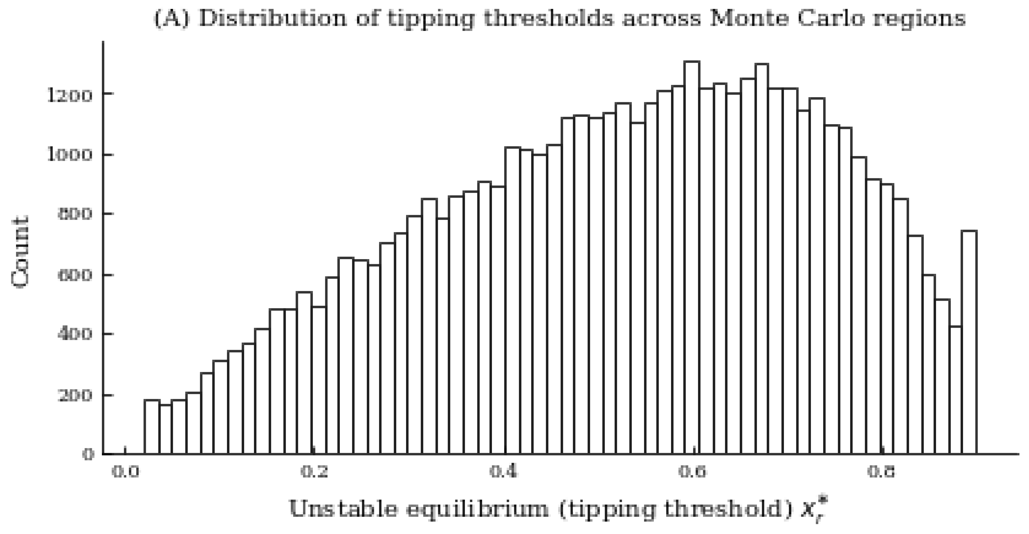
Figure A2.
Monte Carlo relationship between network connectivity (spectral radius proxy ) and the numerically solved tipping threshold . Points show individual regional draws. The solid line is the binned mean; the hatched band shows the 10–90% conditional range. Consistent with the model’s comparative statics, more connected regions tend to require a lower critical mass for take-off.
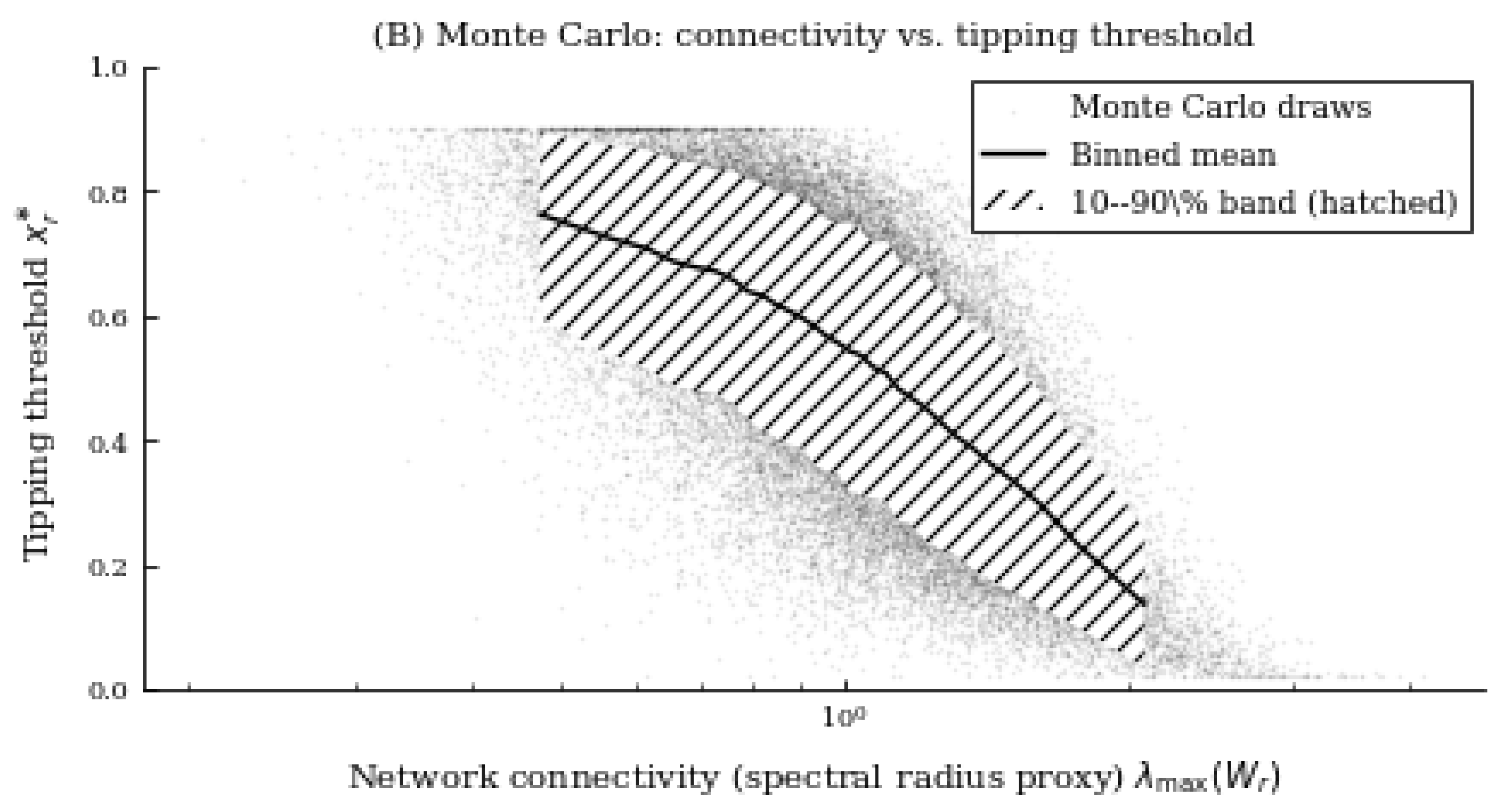
Figure A3.
Partial dependence of the numerically solved tipping threshold on network connectivity , holding operating costs and infrastructure at their sample medians. The downward slope visualises the theoretical prediction that stronger peer/network spillovers lower the critical mass required for the transition to the high-adoption regime.
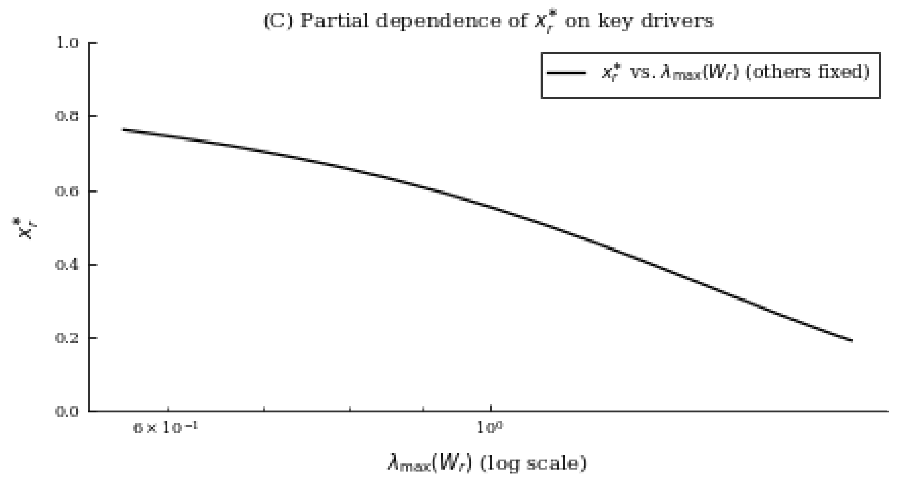
Figure A4.
Illustrative Filippov-style adoption trajectory with explicit regime switching. During the initial phase (hatched region), a subsidy is active and adoption grows. After subsidy removal, the vector field switches and growth slows; when adoption exceeds a capacity proxy, the trajectory enters a bottleneck regime (markers), capturing non-smooth constraint-induced dynamics discussed in the model.
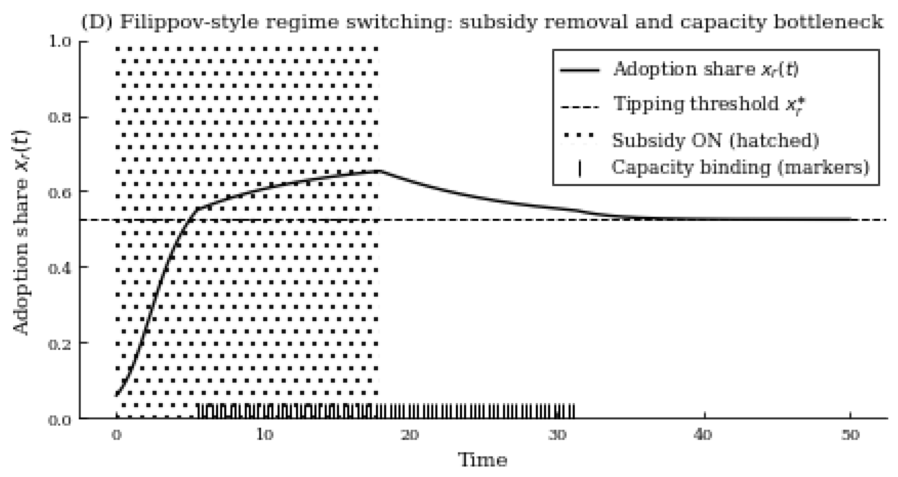

Table A1.
Monte Carlo Simulation Algorithm.
| ine Step | Description |
|---|---|
| ine 1 | Draw regional characteristics from their respective distributions. |
| 2 | For each region r, construct the adoption drift with two stable equilibria and one interior unstable equilibrium. |
| 3 | Numerically solve for the unstable equilibrium using a bracketing and bisection method. |
| 4 | Store and compute summary statistics and conditional moments (binned means and quantiles). |
| 5 | Select a representative region and simulate the hybrid time path under regime switching. |
| 6 | Activate subsidy regime while policy is in force; switch vector field when the subsidy is removed. |
| 7 | Impose capacity-binding regime once adoption exceeds a threshold, generating Filippov-type switching dynamics. |
| 8 | Generate figures: distribution of , cross-sectional relationships, partial dependence, and regime-switching trajectories. |
| ine |
Notes: The interior equilibrium is unstable and represents the critical adoption threshold required for transition to the high-adoption regime. Regime switching follows a Filippov-type hybrid system with piecewise-defined vector fields.
Table A2.
Simulation Parameters and Calibration Choices.
| ine Parameter | Description | Value / Distribution | Role |
|---|---|---|---|
| ine N | Number of Monte Carlo draws | Cross-sectional heterogeneity | |
| Network connectivity (spectral radius) | Peer/network spillovers | ||
| EV operating cost index | Adoption disincentives | ||
| Effective charging infrastructure | Complementary investment | ||
| Lower stable equilibrium | Low-adoption regime | ||
| Upper stable equilibrium | High-adoption regime | ||
| Drift curvature parameter | Speed of adjustment | ||
| s | Subsidy intensity (when active) | Policy support | |
| Subsidy removal time | 18 | Policy horizon | |
| Capacity-binding threshold | Supply bottleneck | ||
| Time step (trajectory simulation) | Numerical integration | ||
| T | Simulation horizon | 50 | Dynamic illustration |
| ine |
Notes: Parameter values are chosen to generate a well-defined bistable adoption structure with an interior unstable equilibrium. Distributions reflect heterogeneity across regions rather than calibrated point estimates. Results are robust to moderate perturbations of parameter values.
Table A3.
Monte Carlo Summary Statistics
| ine Variable | Obs. | Mean | Std. Dev. | Min | 25th pct. | Median | 75th pct. | Max |
|---|---|---|---|---|---|---|---|---|
| ine Network connectivity | 50,000 | 1.061 | 0.380 | 0.207 | 0.790 | 0.998 | 1.265 | 4.144 |
| Operating cost index | 50,000 | 1.001 | 0.200 | 0.213 | 0.867 | 1.000 | 1.134 | 1.759 |
| Infrastructure index | 50,000 | 1.085 | 0.454 | 0.198 | 0.764 | 1.002 | 1.310 | 6.105 |
| Tipping threshold | 50,000 | 0.526 | 0.210 | 0.020 | 0.371 | 0.545 | 0.694 | 0.900 |
| ine |
Notes: Each observation corresponds to one Monte Carlo draw representing a heterogeneous region. denotes the spectral radius of the regional interaction network, is the EV operating cost index, is effective charging infrastructure, and is the numerically solved unstable equilibrium (tipping threshold). The sample correlation between and is .
References
- Casals, Lluc Canals, et al. Sustainability analysis of the electric vehicle use in Europe for CO2 emissions reduction. Journal of Cleaner Production 2016, 127, 425–437. [CrossRef]
- Zaino, Rami, et al. Electric vehicle adoption: A comprehensive systematic review of technological, environmental, organizational and policy impacts. World Electric Vehicle Journal 2024, 15, 375. [CrossRef]
- Chi, Junwook. Impacts of electric vehicles and environmental policy stringency on transport CO2 emissions. Case Studies on Transport Policy 2025, 19, 101330. [CrossRef]
- Monteiro, L.H.A. A simple overview of complex systems and complexity measures. Complexities 2025, 1, 2. [Google Scholar] [CrossRef]
- Sierzchula, William, Sjoerd Bakker, Kees Maat, and Bert van Wee. The influence of financial incentives and other socio-economic factors on electric vehicle adoption. Energy Policy 2014, 68, 183–194. [CrossRef]
- Gerber Machado, Pedro; et al. Electric vehicles adoption: A systematic review (2016–2020). Wiley Interdisciplinary Reviews: Energy and Environment 2023, 12, e477. [CrossRef]
- Bryła, Paweł, Shuvam Chatterjee, and Beata Ciabiada-Bryła. Consumer adoption of electric vehicles: A systematic literature review. Energies 2022, 16, 205. [CrossRef]
- Rahman, Md Mokhlesur and Jean-Claude Thill. A comprehensive survey of the key determinants of electric vehicle adoption: Challenges and opportunities in the smart city context. World Electric Vehicle Journal 2024, 15, 588. [CrossRef]
- Yang, Y.; Tan, Z. Investigating the influence of consumer behavior and governmental policy on the diffusion of electric vehicles in Beijing, China. Sustainability 2019, 11, 6967. [Google Scholar] [CrossRef]
- Jia, C.; Ding, C.; Chen, W. Research on the diffusion model of electric vehicle quantity considering individual choice. Energies 2023, 16, 5423. [Google Scholar] [CrossRef]
- van Dijk, Jeremy; Delacrétaz, Nathan; Lanz, Bruno. Technology adoption and early network infrastructure provision in the market for electric vehicles. Environmental and Resource Economics 2022, 83, 631–679. [CrossRef]
- Zhang, Xiang; et al. Direct network effects in electric vehicle adoption. Technological Forecasting and Social Change 2024, 209, 123770. [CrossRef]
- Caroleo, Brunella; Pautasso, Elisa; Osella, Michele; Palumbo, Enrico; Ferro, Enrico. Assessing the Impacts of Electric Vehicles Uptake: A System Dynamics Approach. In 2017 IEEE 41st Annual Computer Software and Applications Conference (COMPSAC), vol. 2, IEEE, 2017; pp. 790–795. [CrossRef]
- Li, Jingjing; Nian, Victor; Jiao, Jianling. Diffusion and benefits evaluation of electric vehicles under policy interventions based on a multiagent system dynamics model. Applied Energy 2022, 309, 118430. [CrossRef]
- Limoochi, Arham and Javier Rodriguez. EVs meet health: A complex-systems policy integration approach for electric vehicle adoption and its impact on respiratory and cardiovascular disease. Journal of Transport & Health 2024, 39, 101921. [CrossRef]
- Zolfagharian, Mohammadreza; et al.Toward the dynamic modeling of transition problems: The case of electric mobility. Sustainability 2020, 13, 38. [CrossRef]
- Baxter, G. J.; Dorogovtsev, S. N.; Goltsev, A. V.; Mendes, J. F. F. Bootstrap percolation on complex networks. Physical Review E 2010, 82, 011103. [Google Scholar] [CrossRef]
- Baxter, G. J.; Dorogovtsev, S. N.; Goltsev, A. V.; Mendes, J. F. F. Avalanche collapse of interdependent networks. Physical Review Letters 2012, 109, 248701. [Google Scholar] [CrossRef] [PubMed]
- Petitjean, H.; Finck, S.; Schmoll, P.; Charlet, A. The concept of homeodynamics in systems theory. Complexities 2025, 1, 6. [Google Scholar] [CrossRef]
- Baia, M.; Bagnoli, F.; Matteuzzi, T. Forecasting chaotic dynamics using a hybrid system. Complexities 2025, 1, 5. [Google Scholar] [CrossRef]
- Filippov, A. F. Differential Equations with Discontinuous Righthand Sides; Kluwer Academic Publishers, 1988. [Google Scholar] [CrossRef]
- Stiefenhofer, P. Exponential stability of nonsmooth periodic orbits in the complex space. Physics Letters A 2025, 560, 130935. [Google Scholar] [CrossRef]
- Stiefenhofer, P. Contraction and periodic orbits in time-periodic Filippov systems. Annals of Mathematical Physics 2025, 8, 166–176. [Google Scholar] [CrossRef]
- Stiefenhofer, P. Spectral contraction framework for planar Filippov systems: Existence and stability of nonsmooth periodic orbits. Communications in Advanced Mathematical Sciences 2025, 8, 189–209. [Google Scholar] [CrossRef]
- Breschi, Valentina, et al. Social network analysis of electric vehicles adoption: A data-based approach. In 2020 IEEE International Conference on Human-Machine Systems (ICHMS), IEEE, 2020. [CrossRef]
- Mekky, Maher F. and Alan R. Collins. The impact of state policies on electric vehicle adoption – a panel data analysis. Renewable and Sustainable Energy Reviews 2024, 191, 114014. [CrossRef]
- Mesquita, Andressa Rosa, et al. Barriers to electric vehicle adoption: A framework to accelerate the transition to sustainable mobility. Sustainability 2025, 17, 8318. [CrossRef]
- Breschi, Valentina, et al. Fostering the mass adoption of electric vehicles: A network-based approach. IEEE Transactions on Control of Network Systems 2022, 9, 1666–1678. [CrossRef]
- Abas, Pg Emeroylariffion and Benedict Tan. Modeling the impact of different policies on electric vehicle adoption: An investigative study. World Electric Vehicle Journal 2024, 15, 52. [CrossRef]
- Xiang, Yue, et al. Scale evolution of electric vehicles: A system dynamics approach. IEEE Access 2017, 5, 8859–8868. [CrossRef]
- Singh, Divya, Ujjwal Kanti Paul, and Neeraj Pandey. Does electric vehicle adoption (EVA) contribute to clean energy? Bibliometric insights and future research agenda. Cleaner and Responsible Consumption 2023, 8, 100099. [CrossRef]
- Singh, Gaurvendra, et al. Electric vehicle adoption and sustainability: Insights from the bibliometric analysis, cluster analysis, and morphology analysis. Operations Management Research 2024, 17, 635–659. [CrossRef]
- Li, Jingjing, Jianling Jiao, and Yunshu Tang. Analysis of the impact of policies intervention on electric vehicles adoption considering information transmission – based on consumer network model. Energy Policy 2020, 144, 111560. [CrossRef]
- Zhang, Qi, et al. Market adoption simulation of electric vehicle based on social network model considering nudge policies. Energy 2022, 259, 124984. [CrossRef]
- Ma, J.; Zhu, Y.; Chen, D.; Zhang, C.; Song, M.; Zhang, H.; Zhang, K. Analysis of urban electric vehicle adoption based on operating costs in urban transportation network. Systems 2023, 11, 149. [Google Scholar] [CrossRef]
Disclaimer/Publisher’s Note: The statements, opinions and data contained in all publications are solely those of the individual author(s) and contributor(s) and not of MDPI and/or the editor(s). MDPI and/or the editor(s) disclaim responsibility for any injury to people or property resulting from any ideas, methods, instructions or products referred to in the content. |
© 2026 by the authors. Licensee MDPI, Basel, Switzerland. This article is an open access article distributed under the terms and conditions of the Creative Commons Attribution (CC BY) license (http://creativecommons.org/licenses/by/4.0/).
Copyright: This open access article is published under a Creative Commons CC BY 4.0 license, which permit the free download, distribution, and reuse, provided that the author and preprint are cited in any reuse.


