
Submitted:
09 January 2026
Posted:
12 January 2026
You are already at the latest version
Abstract
Robust radar object classification is a challenging task, primarily due to the aspect sensitivity limitation of one-dimensional High-Resolution Range Profile (HRRP) data. To address this, we propose Point-HRRP-Net. This multi-modal framework integrates HRRP with 3D LiDAR point clouds via a Bi-Directional Cross-Attention (Bi-CA) mechanism to enable deep feature interaction. Since paired real-world data is scarce, we constructed a high-fidelity simulation dataset to validate our approach. Experiments conducted under strict angular separation demonstrated that Point-HRRP-Net consistently outperformed single-modality baselines. Our results also verified the effectiveness of Dynamic Graph CNN (DGCNN) for feature extraction and highlighted the high inference speed and the potential of Mamba- based architectures for future efficient designs. Finally, this work validates the feasibility of the proposed approach in simulated environments, establishing a foundation for robust object classification in real-world scenarios.
Keywords:
radar perception
; object classification
; High-Resolution Range Profile (HRRP)
; point cloud
; multi-modal fusion
; cross-attention
1. Introduction
Radar object classification is critical for remote sensing [1,2]. As a classic data source, one-dimensional High-Resolution Range Profile (HRRP) is characterized by its ease of acquisition, low dimensionality, and efficient processing. [3,4,5].
Early HRRP recognition technologies relied heavily on "hand-crafted features" [6,7]. Researchers attempted to extract feature vectors from HRRP using methods like template matching and statistical models (e.g., Hidden Markov Models) [8,9]. However, restricted by shallow feature extraction and heavy reliance on prior knowledge, these methods often struggle to generalize to unseen orientations. [10,11,12]. The emergence of deep learning has addressed these limitations by enabling automatic feature extraction [13]. Researchers initially applied Convolutional Neural Networks (CNNs) [14] to HRRP, treating them as 1D signals to extract local scattering features. To address the inherent sequential dependencies of radar echoes, scholars subsequently employed Recurrent Neural Networks (RNNs) [15,16] and variants like LSTM [17] and GRU [18]. However, these architectures often fail to capture long-range dependencies [19]. This challenge prompted the adoption of the Transformer [20], which utilizes self-attention to model global context with superior parallel efficiency [21,22]. More recently, the field has witnessed the emergence of advanced architectures: the Conformer [23] integrates CNNs and Transformers to simultaneously capture local and global features, while the Mamba framework [24], based on State Space Models (SSM), offers linear computational complexity. Specifically, 1D-Mamba [25] has shown great potential in efficiently processing long HRRP sequences. However, generating HRRP inevitably collapses 3D structures into 1D signals. This compression causes significant information loss, which severely limits generalization to unseen angles. Existing single-modality approaches fail to fundamentally address the limitation.
To overcome this, scholars have turned to multi-modal fusion to incorporate complementary information. For instance, researchers have combined Synthetic Aperture Radar (SAR) [26,27] with optical images to enable all-weather, high-precision ground target recognition. Others have integrated HRRP with micro-Doppler features to refine the distinction of target motion states [28]. For airborne target identification, studies have explored fusing HRRP with Infrared (IR) images [29,30]. In autonomous driving, fusing millimeter-wave radar with LiDAR is widely adopted [31,32]. However, a fundamental distinction exists: millimeter-wave radar provides 3D spatial data, whereas HRRP consists solely of 1D signatures. Consequently, the fusion of LiDAR and HRRP remains largely unexplored.
Advancements in LiDAR technology [33] have made acquiring 3D LiDAR point clouds from distant targets a reality. Since point clouds preserve intrinsic geometric topology that remains invariant under rigid motion [34], they serve as an ideal candidate for fusion with HRRP. Regarding processing methods, PointNet[35] and PointNet++ [36] pioneered direct learning on unordered points, bypassing inefficient voxelization [37,38,39]. Subsequently, Dynamic Graph CNN (DGCNN) [40] introduced dynamic graph convolution to capture local topology, while Point Transformer [20] and PointMLP [41] introduced self-attention and pure residual designs, respectively. Most recently, the Mamba framework has extended its success to the 3D domain. Specifically, PointMamba [42] adapts the SSM mechanism to point clouds, achieving a superior balance between performance and computational efficiency.
Conversely, HRRP provides scattering information that resolves geometric ambiguities caused by point cloud occlusions. As shown in Figure 1, when the line of sight directly faces the base, the cone, cylinder, and cone-cylinder assembly all appear as identical circles [Figure 1a–c]. This makes them indistinguishable based on shape alone. However, their corresponding HRRP remains distinct due to specific scattering mechanisms like edge diffraction [Figure 1d–f].
Traditional strategies like early and late fusion fail to capture deep feature interactions due to their shallow interaction mechanisms. [43,44]. To address this, the field shifted toward intermediate fusion to enable complex feature interactions [45,46,47]. Specifically, cross-attention mechanisms were introduced for fine-grained feature alignment [48,49]. Concurrently, to alleviate the computational burden of standard attention, efficiency-oriented designs have emerged, including Linear-Attention [50], Efficient-Attention [51], and the recent Mamba architecture [52]. These models utilize linear-complexity mechanisms to accelerate inference. In this work, to establish explicit, point-to-point interactions between HRRP and 3D point clouds for robust recognition, we propose Point-HRRP-Net. This framework leverages a Bi-Directional Cross-Attention (Bi-CA) mechanism to improve classification accuracy and generalization capability.
The main contributions of this paper are summarized as follows:
- HRRP is distinct from millimeter-wave radar. To the best of our knowledge, this is the first framework to fuse HRRP with 3D point clouds for object classification.
- We propose Point-HRRP-Net, a fusion framework that incorporates a Bi-CA mechanism to integrate HRRP and 3D point clouds.
- We have constructed and publicly released a paired point cloud-HRRP dataset through electromagnetic and optical simulation.
- Experimental results in a simulated environment demonstrate that the proposed framework outperforms single-modality baselines. Comprehensive ablation studies validate the design rationale, demonstrating the necessity of both the specific feature extractors and the Bi-CA mechanism for achieving robust performance.
2. Methods
2.1. Point-HRRP-Net Overview
The overall architecture of our proposed network is illustrated in Figure 2. The data processing pipeline can be conceptually divided into three main stages: (1) dual-branch feature extraction, (2) Bi-CA fusion, and (3) classification.
The process begins by normalizing the HRRP and point cloud inputs. Subsequently, these modalities are processed in parallel by specialized feature extractors. Specifically, the HRRP branch analyzes in both the time and frequency domains using a hybrid CNN-Transformer architecture, while the point cloud is encoded by a DGCNN-based extractor to capture geometric features. The extracted feature sequences are then fused via the Bi-CA mechanism to enable explicit cross-modal interaction. Finally, the fused features are aggregated through pooling and concatenation, and subsequently fed into an MLP for classification.
2.2. HRRP Feature Extractor
As shown in Figure 3, we propose a dual-stream extractor to capture target characteristics from both time and frequency domains. One stream processes the raw HRRP to analyze time-domain scattering distributions, while the other processes the amplitude spectrum (derived via FFT) to encode frequency-domain attributes. The extracted features from both branches are then projected and concatenated into a unified HRRP feature sequence, which serves as the input for the subsequent fusion module.
The time-domain branch processes the raw HRRP directly. Let the input be represented as a vector , where denotes the number of range bins. To capture local scattering patterns, we employ a hierarchical 1D-CNN backbone. This network consists of stacked convolutional blocks, each comprising 1D convolution layers followed by Max-Pooling. This design enables the extraction of features at varying scales, efficiently encoding both detailed peaks and global structural semantics.
The data flow through the time-domain 1D-CNN is detailed in Figure 4. Specifically, the hierarchical architecture comprises three main blocks with increasing channel depths (8, 16, and 32 filters, respectively). The input tensor, with a shape of () where B is the batch size, is first processed by two convolutional layers with 8 filters, followed by a Max-Pooling operation that halves the sequence length. This process is repeated with deeper feature maps. The 1D convolution operation at a layer k can be formally expressed as:
where is the input feature map from the previous layer, and are the learnable filter weights and biases, * denotes the 1D convolution with padding, and is the ReLU activation function. The subsequent Max-Pooling operation reduces the dimensionality and provides local translational invariance. After passing through the 1D-CNN backbone, the raw HRRP is transformed into a compact sequence of high-level feature vectors , where is the reduced sequence length and is the final channel dimension (32 in this case).
Following local feature extraction by the 1D-CNN, the sequence is fed into a Transformer Encoder. Unlike 1D-CNNs, which are limited by local receptive fields, the Transformer utilizes multi-head self-attention to capture global dependencies among scattering centers. This mechanism dynamically weights the importance of all elements in the sequence, effectively modeling the target’s global context. The output is an enriched time-domain feature sequence , where .
Concurrently, the second stream processes the frequency-domain information. The amplitude spectrum of the HRRP is first obtained via Fast Fourier Transform (FFT) and taking the absolute value:
where denotes the FFT operator. This spectrum is then processed by an analogous architecture consisting of a hierarchical 1D-CNN and a Transformer Encoder. For efficiency, we employ a lightweight 1D-CNN architecture ((2, 4), (2, 8), (1, 16)) to extract salient spectral features. This yields a frequency-domain feature sequence , where is set to 16.
The final step is Feature Unification. Since the feature sequences and have differing dimensions ( and ), they are projected into a unified feature space of dimension using separate linear layers:
where are learnable weight matrices and are learnable bias vectors. This projection ensures dimensional compatibility. Finally, the mapped sequences are concatenated along the length dimension to produce the unified HRRP representation . This sequence serves as the input for the subsequent fusion module.
2.3. 3D Point Cloud Feature Extractor: DGCNN
To mitigate the aspect sensitivity inherent in HRRP, we utilize point clouds to provide rotation-invariant geometric context. We employ a DGCNN [40] as the feature backbone. Unlike architectures operating on fixed grids, DGCNN dynamically constructs local neighborhood graphs in the feature space, enabling the effective capture of fine-grained topological structures regardless of the target’s pose.
Subsequently, for a given point cloud input with points, we represent each point by a feature vector (initially its 3D coordinates). At each layer, we construct a local geometric structure by identifying the nearest neighbors (k-NN) for every point. Crucially, this graph is dynamically updated at each network depth, allowing the model to group points based on learned semantic similarities rather than just physical proximity.
The core operation is the EdgeConv block, which computes "edge features" describing the relationship between the central point and its neighbors . To capture both local geometry and global position, we formulate the edge feature as:
where denotes concatenation. Here, encodes the local neighborhood structure, while preserves absolute spatial information. These features are processed by a shared-weight Multi-Layer Perceptron (MLP), implemented efficiently as a 1×1 convolution. Finally, a channel-wise symmetric function (Max-Pooling) aggregates information from the local neighborhood, ensuring permutation invariance. This operation is defined as:
where represents the set of edges in the dynamically constructed graph, and denotes the learnable MLP.
To preserve geometric information across different abstraction levels, we aggregate the outputs from all stacked EdgeConv blocks. Specifically, the intermediate feature maps are concatenated along the channel dimension. This skip-connection design effectively integrates fine-grained local details from shallow layers with global semantic contexts from deep layers.
Following feature aggregation, a shared MLP (implemented as a 1D convolution) projects the combined features into a high-dimensional embedding space. The final output of the point cloud branch is a feature sequence , where is the number of points and . This sequence provides the rotation-invariant geometric representation required for the subsequent Bi-CA fusion module.
2.4. Bi-CA Fusion Module
To effectively fuse the heterogeneous HRRP and point cloud features, we introduce a Bi-CA mechanism. This approach allows each modality to dynamically query the other, thereby selectively integrating complementary information.
Prior to fusion, we must map the input features into a shared latent space. Let the output sequence from the point cloud extractor be denoted as (where ), and the unified sequence from the HRRP extractor as (where ). To align these features within a shared semantic space, we project both modalities to a common dimension using separate learnable linear layers.
Formally, this projection is defined as:
where and are learnable weight matrices, and and are the corresponding bias vectors, where and are the aligned feature sequences serving as inputs for the fusion module. As illustrated in Figure 5, the first stream utilizes the aligned point cloud features to generate the Query vectors , while the HRRP features are projected to produce the Key and Value vectors. The attention mechanism dynamically aggregates electromagnetic information for each geometric point:
The geometric representation is then updated via a residual connection and Layer Normalization:
This process effectively enriches the point cloud representation by selectively integrating complementary HRRP cues, yielding more discriminative geometric features. Symmetrically, the HRRP-enrichment stream employs as the Query and as the Keys and Values to ground abstract radar signals into the 3D geometric context, following the same formulation as Equation (9) and (10).
To facilitate deep feature interaction, we stack layers with 8 attention heads, a choice validated by the sensitivity analysis in Appendix Figure A1. The refined feature sequences are aggregated via Global Average Pooling (GAP) and concatenated to form a unified vector , which is fed into an MLP classifier. Regarding the attention configuration, we adopt a Post-Norm design (normalization after residual connection) to ensure training stability and forgo causal masking to maintain a global receptive field for effective bidirectional modeling.
2.5. Experimental Setup and Implementation Details
All model training and accuracy evaluations were conducted on a Windows platform equipped with an NVIDIA RTX 5070 GPU (Blackwell Architecture).
To ensure fair efficiency comparisons, we evaluated inference latency, FLOPs, and parameter counts on a Linux workstation powered by an NVIDIA RTX 4090. This hardware transition was necessitated by the Mamba-based baselines, which rely on the mamba-ssm library’s optimized CUDA kernels. These kernels require specific environment configurations (Linux OS and mature CUDA versions) that currently face compatibility constraints on the RTX 50 series architecture.
For model optimization, we employed the Adam optimizer with a weight decay of 1e-5. A differential learning rate strategy was adopted to accommodate the distinct characteristics of different network components. Specifically, the learning rates for the HRRP feature extractor and the point cloud feature extractor were set to 3e-4 and 5e-4, respectively. The remaining modules, including the feature mapping layers, the cross-attention layers, and the final classifier, were assigned a learning rate of 1e-4. All models were trained with a batch size of 32. For a fair comparison, we employed an early stopping protocol to ensure convergence. The training process was terminated if the validation loss did not decrease for 20 consecutive epochs. The model checkpoint corresponding to the lowest validation loss was then selected for the final evaluation.
3. Results
3.1. Dataset Setup
3.1.1. Target Geometry and Parameters
Direct acquisition of measured electromagnetic data is difficult [53,54]. Our research requires a dataset containing paired point cloud and HRRP data. However, existing public datasets are often mismatched in terms of objects, environments, or viewpoints [55,56,57]. It is practically infeasible to generate simulated data for another modality that pairs with existing real-world samples. To address this issue, we constructed a dataset specifically for this task through high-fidelity electromagnetic and optical simulations.
We selected three representative classes of Perfect Electrical Conductor (PEC) targets. Following precedents in related literature on object classification [58], our selection comprises cones, cylinders, and composite objects formed by an upper cone and a lower cylinder. These targets serve as fundamental geometric primitives of more complex objects, providing a foundational and challenging test case for recognition algorithms. Furthermore, their scattering characteristics cover a wide range of typical electromagnetic phenomena—including scattering from tips, edges, curved surfaces, and geometric discontinuities—thus making them broadly representative for robustness evaluation.
The geometric configuration and dimensional parameters of the targets are illustrated in Figure 6 and Figure 7. Figure 6 defines the observation geometry, illustrating the coordinate system and the incident angle, , which represents the line-of-sight direction relative to the target’s primary axis. The detailed longitudinal cross-sections and specific dimensions of these targets are provided in Figure 7. To ensure numerical stability and avoid meshing singularities during the electromagnetic simulation, the mathematically sharp tips of the cone and the cone-cylinder composite were regularized by replacing them with small paraboloids. The paraboloid for the single cone target was defined with a focal length of 0.0025 m, while that of the composite object’s tip utilized a focal length of 0.004 m.
3.1.2. Multimodal Data Simulation
1D HRRP Data: We employed the electromagnetic simulation software FEKO to generate the HRRP data. In the simulation, the target surfaces were set as PEC, and a wideband signal with a center frequency of 6 GHz and a bandwidth of 4 GHz (ranging from 4 to 8 GHz) was used for excitation. The signal was a stepped-frequency waveform with a frequency step of 50 MHz.
The theoretical range resolution, , is determined by the signal bandwidth, B, according to
where c is the speed of light. The maximum unambiguous range, , is determined by the frequency step, , as
According to Equations (11) and (12), the calculated range resolution is 3.75 cm, which is sufficient to capture the fine structural information of the targets, and the unambiguous range is 3 m, which completely encompasses the targets with an adequate margin. Considering that all three target types are bodies of revolution, we sampled them uniformly along the elevation angle () from 0° to 180° at 1° intervals, generating a total of 543 raw HRRP samples (181 angles for each of the three target types).
We designed a Python algorithm to generate the 3D point clouds of the targets by simulating LiDAR illumination on their 3D surfaces and capturing the reflected sparse point clouds. The viewpoints for point cloud generation were strictly aligned with the observation angles of the HRRP simulations. The raw point clouds were then uniformly down-sampled to a set of 256 points, resulting in 543 raw point cloud samples that are strictly paired with the HRRP.
3.1.3. Data Augmentation and Dataset Splitting
Data Augmentation and Scaling: To enhance model robustness and expand the dataset, we designed a joint data augmentation scheme comprising 15 distinct strategies, such as Gaussian noise injection, coordinate jittering, and global scaling. Detailed configurations for each strategy are provided in Appendix A (Table A1 ). Through these operations, the original 543 data pairs were expanded to a total of 8,688 samples (543 × 16). Prior to training, all HRRP data underwent Min-Max normalization, while point clouds were centered and normalized to fit within a unit cube.
Dataset Splitting: To rigorously evaluate generalization capability to unseen viewpoints, we adopted a structured, angle-based splitting strategy. The observation range from 1° to 180° was partitioned into contiguous, non-overlapping angular blocks. Within each block, data were divided into training, validation, and test sets according to a 5:2:2 ratio. To systematically assess robustness against varying degrees of angular separation, we established six experimental configurations with block sizes ranging from 9°to 180°.
For instance, in the 90° split configuration, the 180° observation range is divided into two blocks (i.e., 1°–90° and 91°–180°). For the first block, the 5:2:2 ratio allocates angles 1°–50° to training, 51°–70° to validation, and 71°–90° to testing. A similar division is applied to the second block. A larger block size imposes greater angular separation, presenting a more challenging generalization task. The sample corresponding to the 0° observation angle was consistently included in the training set across all configurations. Supplementary analysis (Appendix D, Figure A2) indicates that excluding samples causes a negligible accuracy drop (< 0.8%), ruling out potential data leakage from back-scattering symmetry.
3.1.4. Evaluation Metrics
To comprehensively evaluate the classification performance, we employ two standard metrics: Overall Accuracy (OA) and F1-Score. Accuracy serves as the primary metric for the general performance comparisons presented in Table 1. Additionally, given the potential for geometric confusion between target classes at specific viewpoints, we utilize the F1-Score (the harmonic mean of Precision and Recall) in our ablation studies (Table 2 and Table 3). This metric provides a more robust assessment of the model’s ability to balance precision and recall, ensuring that the performance improvements are not biased towards specific classes.
We also evaluate its efficiency from three perspectives:
Parameters (Params): We calculate the number of trainable parameters of the entire model, measured in millions (M), to quantify the model’s size and memory footprint.
FLOPs (G): This metric quantifies the number of operations required for a single forward pass, measured in GFLOPs.
Latency (ms): Latency metrics in this paper represent the inference time of a single sample (batch size = 1). Unless otherwise specified, results are reported on an NVIDIA GeForce RTX 4090 GPU.
We conducted comprehensive inference latency benchmarks across a wide range of hardware to assess deployment feasibility. As detailed in Table A2, our tests spanned from data center accelerators to consumer-grade GPUs.
For edge deployment, we specifically utilized the NVIDIA Jetson Orin Nano (8GB). The experimental environment on this embedded platform was configured with Ubuntu 22.04 LTS and CUDA 12.6.68. Operating under the 15 W power mode, the embedded platform achieved an average inference latency of 33.29 ms. This result indicates that the proposed model possesses favorable deployment capabilities, with acceptable inference speeds on embedded platforms.
3.2. Experimental Results
In this section, we evaluate Point-HRRP-Net from three perspectives: (1) comparison with single-modality baselines to assess generalization; (2) ablation studies on fusion strategies to validate the cross-attention mechanism; and (3) analysis of the feature extractor to justify our architectural choices.
3.2.1. Performance Comparison against Single-Modality Methods
Table 1 presents the generalization performance comparison of Point-HRRP-Net against eight representative single-modality methods under six angle-based split configurations. These include our baseline HRRP network (HRRP-only), the MSDP-Net, Point-Transformer, and DGCNN, as well as the recent advanced Transformer-style network (Conformer) and Mamba-style networks (1D-Mamba and PointMamba). A vertical comparison of accuracy reveals that the multi-modal framework consistently outperformed single-modality methods across both small and large angle dataset splits. Specifically, under the split configuration, our multi-modal model achieved a peak accuracy of 97.51%.
As the angular separation of the dataset splits increased from to , the overall recognition performance of all models exhibited an expected downward trend. A horizontal comparison indicates that Point-HRRP-Net demonstrated excellent robustness under large viewpoint changes. In the split, Point-HRRP-Net maintained an accuracy of 57.67%, surpassing all baseline models. It outperformed the baseline HRRP-only by 12.05% and the best-performing point cloud baseline, PointMamba, by 3.87%.
Regarding the single-modality HRRP baselines, performance variations among different architectures were pronounced. Leveraging its powerful sequence modeling capabilities, Conformer achieved the best results among HRRP-based methods on our dataset. For instance, it attained 52.45% accuracy under the split, outperforming both MSDP-Net and 1D-Mamba. Notably, 1D-Mamba showed a distinct advantage on the 90° split, achieving the highest accuracy among HRRP-based methods in this configuration.
Regarding single-modality point cloud methods, PointMamba significantly outperformed the traditional Point-Transformer and DGCNN across all angle splits. This success stemmed from the Mamba architecture’s advantages in long-sequence and global feature extraction. It achieved an accuracy of 53.80% under the split. This result demonstrated PointMamba’s advanced performance and potential.
3.2.2. Ablation Study on Fusion Strategies
To verify the effectiveness of the proposed Bi-CA mechanism, we conducted comparative experiments by replacing this module with eight fusion strategies: Addition, Product, Gating, Self-Attention, Linear Attention, Efficient Attention, and Bi-Mamba. Detailed ablation study results are listed in Table 2.
For the simple fusion strategies (Concatenation, Addition, and Product), experiments showed they maintained a low inference latency between 5.34 ms and 6.00 ms. However, they performed poorly in large-angle scenarios. These methods achieved respectable F1 scores of approximately 93-96% on the 9° split. While this suggests that basic aggregation is viable when viewpoint discrepancies are minimal, their performance declined significantly as the disparity expanded to 45° and 90°. On the 90° split, Concatenation, Product, and Addition achieved F1 scores of 51.77%, 54.69%, and 60.26%, respectively. Even the best among them lagged behind our proposed method by over 5%. This performance indicates that although simple strategies are fast and parameter-efficient, they lack sufficient capacity to fit complex features. Consequently, they suffer from severe robustness deficiencies under extreme conditions.
Regarding the classic Gating and standard Self-Attention mechanisms, Gating introduced weight modulation but only achieved an F1 score of 58.44% on the 90° test set, failing to surpass the 60% threshold. Self-Attention demonstrated high accuracy under the simple 9° angle but suffered a marked decline on the 90° split, with the F1 score dropping to 47.81%. This represents a gap of 17.73% compared to our method (65.54%). Although Self-Attention theoretically possesses strong fitting capabilities due to its large parameter count, this sharp decline suggests that overfitting occurred in this task. Furthermore, the model complexity increased the latency to 6.99 ms, yet failed to provide the expected accuracy gains.
Subsequently, we evaluated fast attention mechanisms: Linear-Attention and Efficient-Attention. Standard Attention scales quadratically () with sequence length. In contrast, these fast variants reduce the cost to complexity through approximation techniques. Experiments showed that while these methods maintained F1 scores of 91-94% on the 9° split, their performance degraded significantly on the 90° split, dropping to 53.70% and 48.54%, respectively. This indicates that while approximation reduced complexity, it also failed to preserve detailed feature information. Moreover, with latencies ranging from 7.6 ms to 8.1 ms, they offered only a marginal speed advantage over our method (8.76 ms).
Finally, we compared the Bi-Mamba fusion strategy. As a representative SSM, the Mamba architecture typically demonstrates superior parameter efficiency and inference speed in long sequence modeling. However, results indicated that Bi-Mamba performed suboptimally in this task. While achieving an F1 score of 95.68% on the 9° split, its score plummeted to 46.09% on the 90° split. This underperformance is likely because Mamba’s linear complexity advantage is maximized in ultra-long sequences, whereas our HRRP (length 512) and point cloud (256 points) data are relatively short sequences. Consequently, Mamba failed to leverage its long-range dependency capabilities. Furthermore, Mamba lacks the explicit token-to-token interaction inherent in attention mechanisms, which resulted in ineffective feature fusion. Bi-Mamba’s inference latency was 8.53 ms, only a negligible advantage over our method (8.76 ms).
Through bi-directional interaction modeling, our method achieved an F1 score of 65.54% on the 90° split, outperforming the second-best method (Addition) by 5.28% and the Self-Attention mechanism by 17.73%. Although this mechanism increased inference latency to 8.76 ms (an increase of approximately 3.4 ms compared to the fastest simple fusion), we consider this latency cost acceptable for radar engineering applications facing complex and dynamic environments.
3.2.3. Ablation Study on Feature Extractors
We conducted a comprehensive ablation study on feature extractors to validate the rationale behind our final architecture. The experimental results are presented in Table 3. By substituting different components, we evaluated the contribution of each part to the overall performance and efficiency.
Regarding HRRP feature extraction, our proposed dual-domain CNN-Transformer demonstrated the best overall performance, achieving an F1-score at 97.47% on the split. Experimental data showed that 1D-Mamba minimized system latency to 6.52 ms, leveraging its unique selective scan mechanism. However, this speed advantage showed limitations when dealing with large viewing angles. Its F1-score on the split was only 50.10%, lower than our model’s 65.54%. Similarly, the Transformer-based Conformer performed well in sequence modeling (58.02% F1-score on ). Yet, it failed to outperform our architecture. Traditional recurrent neural networks (RNN, LSTM, etc.) performed the worst as they struggled to capture complex spatial scattering features in HRRP. Therefore, the CNN-Transformer was the robust choice for balancing high F1 scores and real-time performance in this study.
For point cloud feature extraction, we compared DGCNN against classic methods and emerging lightweight architectures. Experimental results revealed a notable discrepancy between theoretical and actual efficiency. Although PointMamba possessed extremely low theoretical FLOPs (only 0.0871 G), its actual inference latency in the multi-modal framework (13.81 ms) was higher than our method (8.76 ms). This indicates that the theoretical efficiency of the Mamba architecture failed to materialize as actual inference acceleration within the current framework. We attribute this discrepancy to three primary factors: First, point clouds are unordered sets. To utilize the SSM, PointMamba requires point ordering. This index reordering of unstructured data on the GPU can disrupt memory coalescence, leading to latency overhead. Second, the Mamba kernel is still under active development, and its underlying CUDA kernel optimization may not be as mature as DGCNN. Third, Mamba’s linear complexity advantage only becomes significant with very long sequences. In this experiment, the point cloud contained only 256 points, rendering the latency optimization insignificant. Regarding generalization performance, DGCNN maintained a leading position. Its F1-score on the split (65.54%) was significantly better than PointMLP (54.90%) and PointMamba (57.19%). This result demonstrated the advantage of DGCNN’s EdgeConv operation in capturing the local geometric structure of 3D targets.
Finally, it is worth noting that while PointMamba showed strong potential in single-modality tasks (as shown in Table 1), its accuracy dropped within our multi-modal fusion framework. This suggests a challenge in heterogeneous feature alignment when fusing PointMamba-generated features with HRRP features. We attribute this decline not to a lack of information, but to the structural incompatibility introduced by serialization. PointMamba flattens 3D structures into 1D sequences, creating a structural mismatch that complicates alignment with HRRP representations. Given the comprehensive advantages of DGCNN in feature robustness, fusion gain, and inference speed, we selected DGCNN as the point cloud feature extractor for this study.
4. Discussion
4.1. Visual Analysis of Cross-Modal Interactions
We visualized the attention weights in Figure 8 to examine how the two modalities interact. In the heatmaps, yellow regions denote higher attention weights, whereas blue regions indicate lower weights.
When point cloud features serve as the query (Figure 8a,b), the model assigns higher weights to high amplitudes in the HRRP time domain and low-to-mid frequencies in the frequency domain. These high-amplitude peaks correspond to the dominant scattering centers of the object. Notably, extremely low frequencies receive almost no weight. This suggests that even if these components possess high spectral amplitudes, the model does not consider them useful for target classification. Physically, extremely low frequencies correspond to the slowest variations in the range profile structure, representing merely coarse outlines. This indicates that the network can effectively identify and utilize dominant scattering features while suppressing clutter from non-informative low-frequency components.
Conversely, when HRRP features are used as the query (Figure 8c), attention is not uniformly distributed. Instead, it focuses on geometric edges and discontinuities. Compared to smooth surfaces, edges typically provide more discriminative information for classification. It appears that the model has learned to focus on these geometrically significant regions. By weighting these features more heavily, the model achieves more stable classification performance. This explains why the cross-attention mechanism is more robust than simple feature concatenation.
4.2. Sim-to-Real Analysis
4.2.1. Analysis of Rotational Offset Scenarios
In real-world applications, multi-modal inputs are rarely perfectly aligned. To quantify the impact of such imperfections, we conducted a misalignment test using the pre-trained model on the full test set. Specifically, we introduced a rotational offset ranging from to to one modality during the testing phase to simulate varying degrees of rotational offset.
Figure 9 illustrates the results under the split configuration. We observe that when the rotational offset is within the range of to , the accuracy decline is negligible. Subsequently, the accuracy exhibits slight fluctuations but remains consistently above . This suggests that since both modalities describe the same target, the model retains sufficient discriminatory information even with minor misalignments. When the error exceeds , the fluctuations increase and a noticeable decline occurs, which can be attributed to feature conflicts arising from significant discrepancies between the modalities. Nevertheless, the accuracy remains above .
Figure 10 compares the performance across different dataset split configurations. The results for the , , , and splits are similar, showing a generally flat trend with minimal degradation. However, for the split, the decline in accuracy becomes pronounced as the rotational offset increases. In this configuration, the angular separation between the training and test sets is maximal, placing the highest demand on the model’s generalization capability. We infer that the model likely relies on consistent geometric-physical correspondences for inference in these unseen views. When this correspondence is disrupted by misalignment, the performance drop is consequently more significant compared to less challenging configurations.
4.2.2. Model Stress Test Analysis
To quantify the gap between simulation and real-world data to a certain extent, we conducted progressive stress tests on the model trained with the split. Specifically, we divided the stress into four scenarios: (1) HRRP SNR deterioration; (2) Random Point Cloud jitter; (3) Random Point Cloud point dropping; (4) The summation of the previous three scenarios. Therefore, we tested these four conditions and observed the accuracy decline curves.
The test results are shown in Figure 11. The first row on the x-axis represents the Signal-to-Noise Ratio (SNR) of the HRRP, decreasing gradually from 30dB. When the HRRP SNR is -15dB, we consider the signal to be almost obscured by noise. The second row represents the magnitude of random point cloud jitter, whose numerical value directly applies to the normalized point cloud coordinates. The third row represents the degree of random point cloud loss. When the point cloud loss reaches 70%, we can consider the point cloud to be almost unrecognizable. Curves of different colors represent the addition of different noise conditions, and the maroon curve represents the superposition of all three conditions.
The y-axis represents the average accuracy. If noise is added only to the HRRP, even if the noise almost overwhelms the signal, the accuracy can still reach 95%. This suggests that the model may rely more on the geometric branch of the point cloud. However, a notable phenomenon is that even if the HRRP is already buried in noise, the multi-modal accuracy is still higher than the single-modality accuracy in Table 1. We speculate that this is because, during the training process, the point cloud has already learned more robust features through the HRRP. The accuracy decline caused by point cloud jitter and point cloud loss is more severe. We speculate that this is because DGCNN is adopted as the point cloud extraction branch, which is relatively sensitive to the geometric relationship between points and their neighbors.
When the three degradation conditions are superimposed (solid maroon line), the model’s accuracy changes very little within the range from the initial state (SNR=30dB, , Drop=5%) down to the intermediate state (SNR=15dB, , Drop=20%). This indicates that the system possesses a certain degree of noise resistance. Subsequently, as the severity increases, the performance gradually declines. However, even under the most extreme condition (SNR=-15dB, , Drop=70%), the accuracy remains at 66.2%. This indicates that the model did not collapse. We believe that although the effective information available is limited, the model remains capable of making valid classification predictions.
Through this experiment, we can quantify the impact of different levels of noise on model performance. It helps us predict the model’s inference ability on real-world data.
4.3. Limitations and Future Directions
Although the proposed method demonstrates favorable performance in experiments, we acknowledge several primary limitations in the current work.
First is the "Sim-to-Real" gap. Current model validation relies on high-fidelity electromagnetic simulation data. This simulation environment is idealized with a clutter-free background and target materials are simplified as Perfect Electrical Conductors (PEC); and the targets consist only of basic geometric shapes (e.g., cones and cylinders). Furthermore, real-world objects may exhibit non-rigid deformations, and the current rigid-body assumption may limit the model’s effectiveness in dynamic scenarios.
Second, regarding robustness, stress test results indicate that the model tends to rely on the geometric features provided by the point cloud for decision-making. When point cloud quality degrades severely (e.g., due to heavy rain or dense fog causing LiDAR failure), the model’s recognition performance declines significantly.
Third, the system requires strict synchronization. Point-HRRP-Net is a strict end-to-end model, requiring input data to be fixed in dimension and strictly paired. However, in practical sensor systems, radar and LiDAR sampling rates are asynchronous. The current architecture does not yet support asynchronous inputs, nor does it possess inference capabilities when a single modality is missing.
Fourth, a scalability bottleneck exists within the cross-attention mechanism. While the model meets real-time requirements at the current data resolution, we must acknowledge that the computational complexity of cross-attention scales quadratically with sequence length. In more complex real-world scenarios, such as those requiring the processing of high-density point clouds or ultra-high-resolution HRRP, the model’s memory consumption and computational load will increase exponentially.
Finally, we identified a compatibility issue with SSM. While PointMamba demonstrated superior performance in single-modality tasks, its accuracy degraded within our framework. The structural incompatibility between serialized 1D features and HRRP representations hinders the effective fusion of these two modalities.
Addressing these limitations, our future research plan focuses on the following directions: (1) Future work will attempt to use real-world measured data for training and testing; (2) We will investigate new training strategies or loss functions to reduce the over-reliance on a single modality; (3) We will improve the model framework to adapt to the asynchronous sampling rates of radar and LiDAR, and explore single-modality inference mechanisms; (4) We will attempt to introduce lightweight techniques, such as efficient attention variants or model pruning, to balance efficiency and accuracy for resource-constrained scenarios. (5) Given the potential demonstrated by PointMamba in single-modality comparisons, we plan to fuse this information for radar object classification in future work.
5. Conclusions
Radar object classification tasks often suffer from the inherent aspect sensitivity of HRRP. To address this, we propose Point-HRRP-Net, a multi-modal fusion framework. Our method leverages the rotational invariance of 3D point clouds to provide stable geometric information. Through a Bi-CA mechanism, we achieve deep feature interaction, effectively alleviating the limitations of aspect sensitivity. Under rigorous angle-based split testing, the model demonstrates robustness and generalization capabilities that surpass single-modality approaches. However, the gap between our simulation and real-world environments must be acknowledged. Our tests in Section 4.2.1 and Section 4.2.2 demonstrate that model accuracy exhibits a decline under simulated rotational offsets, noise, and instability. Moreover, unforeseen factors in physical environments may introduce additional uncertainties. Consequently, we explicitly caution that the present results are confined to simulation, and a performance degradation of ≥ 10% on real data is conceivable. Future work will aim to bridge the "sim-to-real" gap using measured data. Additionally, we plan to explore optimization schemes for asynchronous inputs and lightweight deployment.
Author Contributions
Conceptualization, Z.Z. and Z.Y.; Methodology, Z.Z.; Software, Z.Z.; Validation, Z.Z., Z.Y. and Y.W.; Formal Analysis, Z.Z., Z.Y. and Y.W.; Investigation, Z.Z.; Data Curation, Z.Z.; Writing—Original Draft Preparation, Z.Z.; Writing—Review & Editing, Z.Z., Z.Y., H.Z., Y.W. and K.M.; Visualization, Z.Z. and Z.Y.; Supervision, H.Z. and K.M.; Project Administration, H.Z.; Funding Acquisition, H.Z. All authors have read and agreed to the published version of the manuscript.
Funding
This study was financially supported in part by the Open Foundation of the State Key Laboratory of Precision Space-time Information Sensing Technology (No.STSL2025-B-04-01(L)) and Sichuan Science and Technology Program (No.2024YFHZ0002).
Data Availability Statement
The dataset presented in this study is openly available on GitHub at https://github.com/zzo-zhao/HRRP-PC-Paired-Dataset.
Conflicts of Interest
The authors declare no conflicts of interest.
Abbreviations
The following abbreviations are used in this manuscript:
| HRRP | High-Resolution Range Profile |
| LiDAR | Light Detection and Ranging |
| Bi-CA | Bi-Directional Cross-Attention |
| DGCNN | Dynamic Graph Convolutional Neural Network |
| CNN | Convolutional Neural Network |
| RNN | Recurrent Neural Network |
| LSTM | Long Short-Term Memory |
| GRU | Gated Recurrent Unit |
| SSM | State Space Model |
| PEC | Perfect Electrical Conductor |
| FFT | Fast Fourier Transform |
| OA | Overall Accuracy |
| SNR | Signal-to-Noise Ratio |
| MLP | Multi-Layer Perceptron |
| SAR | Synthetic Aperture Radar |
| IR | Infrared |
| GAP | Global Average Pooling |
Appendix A. Data Augmentation Strategies

Table A1.
Detailed list of the 15 joint data augmentation strategies.
| Strategy ID | HRRP Augmentation | Point Cloud (PC) Augmentation |
|---|---|---|
| 1 | Gaussian noise () | Gaussian jitter to coordinates () |
| 2 | Gaussian noise () | Gaussian jitter to coordinates () |
| 3 | Gaussian noise () | Gaussian jitter to coordinates () |
| 4 | Gaussian noise () | Gaussian jitter to coordinates () |
| 5 | Amplitude scaling (range: 0.9-1.1) | Global scaling (range: 0.9-1.1) |
| 6 | Linear shifting (zero-padded) | No operation |
| 7 | No operation | Random rotation |
| 8 | Gaussian Noise () + Linear shifting | Rotation + Global scaling (0.9-1.1) |
| 9 | Gaussian Noise () + Linear shifting | Rotation + Global scaling (0.9-1.1) |
| 10 | Gaussian Noise () + Linear shifting | Rotation + Global scaling (0.9-1.1) |
| 11 | Gaussian Noise () + Linear shifting | Rotation + Global scaling (0.9-1.1) |
| 12 | Amplitude Scaling (0.9-1.1) + Linear shifting | Gaussian Jitter () + Rotation |
| 13 | Amplitude Scaling (0.9-1.1) + Linear shifting | Gaussian Jitter () + Rotation |
| 14 | Amplitude Scaling (0.9-1.1) + Linear shifting | Gaussian Jitter () + Rotation |
| 15 | Amplitude Scaling (0.9-1.1) + Linear shifting | Gaussian Jitter () + Rotation |
Appendix B. Hardware Efficiency and Deployment Analysis
Table A2 presents the inference latency of our model on different devices. To ensure a fair comparison, all tests listed below were conducted in a Linux environment. The testing methodology involved measuring the inference time with a batch size of 1. Specifically, we first performed 50 warm-up runs. Then, we repeated the inference 100 times to calculate the final average result.
It is important to note that for lightweight models performing single-sample inference, the GPU load remains relatively low; consequently, CPU performance significantly impacts the overall latency. Since the host CPUs varied across different testing platforms, the data is for reference only.
Table A2.
Inference latency comparison of our model on different devices (Batch Size = 1).
| Category | Device Name | Architecture | Latency (ms) |
|---|---|---|---|
| Consumer GPU | NVIDIA RTX 5090 | Blackwell | 5.75 |
| NVIDIA RTX 5070 | Blackwell | 6.87 | |
| NVIDIA RTX 4090 | Ada Lovelace | 8.76 | |
| NVIDIA RTX 4090 D | Ada Lovelace | 6.52 | |
| NVIDIA RTX 3080 Ti | Ampere | 9.82 | |
| Workstation / Data Center | NVIDIA RTX 6000 Ada | Ada Lovelace | 5.20 |
| NVIDIA H800 | Hopper | 6.26 | |
| NVIDIA H20 | Hopper | 6.33 | |
| NVIDIA A800 (80G) | Ampere | 7.51 | |
| NVIDIA L20 | Ada Lovelace | 5.98 | |
| NVIDIA Tesla V100 (32G) | Volta | 23.28 | |
| NVIDIA RTX A4000 | Ampere | 9.68 | |
| CPU (x86) | Intel Xeon Gold 6459C | Sapphire Rapids | 8.77 |
| AMD Ryzen 7 9700X | Zen 5 | 12.31 | |
| AMD EPYC 9654 | Zen 4 | 19.62 | |
| AMD EPYC 9754 | Zen 4c | 24.65 | |
| Intel Xeon Platinum 8352V | Ice Lake | 32.90 | |
| Embedded GPU | NVIDIA Jetson Orin Nano (8GB) | Ampere | 33.29 |
| NPU | Huawei Ascend 910B2 | Da Vinci | 241.28* |
*Note: The high latency on the NPU is primarily attributed to the non-optimized kernel within the CANN framework.
Appendix C. Sensitivity Analysis
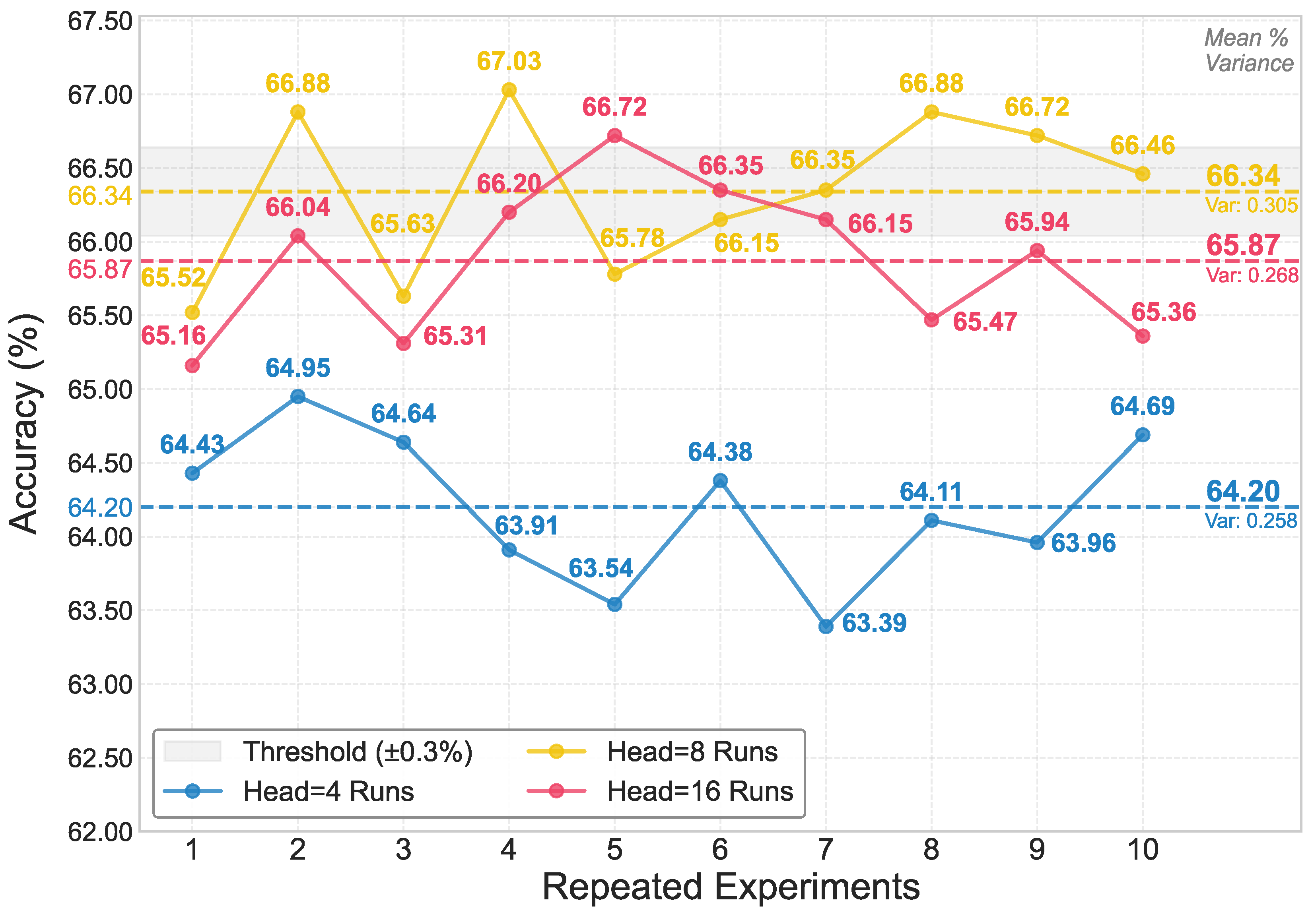
We conducted a sensitivity analysis to investigate the impact of the number of attention heads on model accuracy. By employing different random seeds, we repeated the experiments ten times to calculate the mean classification accuracy on the 90° split. As shown in Figure A1, we compared configurations with 4, 8, and 16 heads. The results indicate that the model achieves optimal accuracy with 8 attention heads. Furthermore, to evaluate the stability, we reported the variance for each configuration (0.258 for 4 heads, 0.305 for 8 heads, and 0.268 for 16 heads).
Figure A1.
Sensitivity analysis of the number of attention heads versus classification accuracy on the 90° split test set.
Figure A1.
Sensitivity analysis of the number of attention heads versus classification accuracy on the 90° split test set.
Appendix D. Analysis of Potential Data Leakage from Back-scattering Symmetry
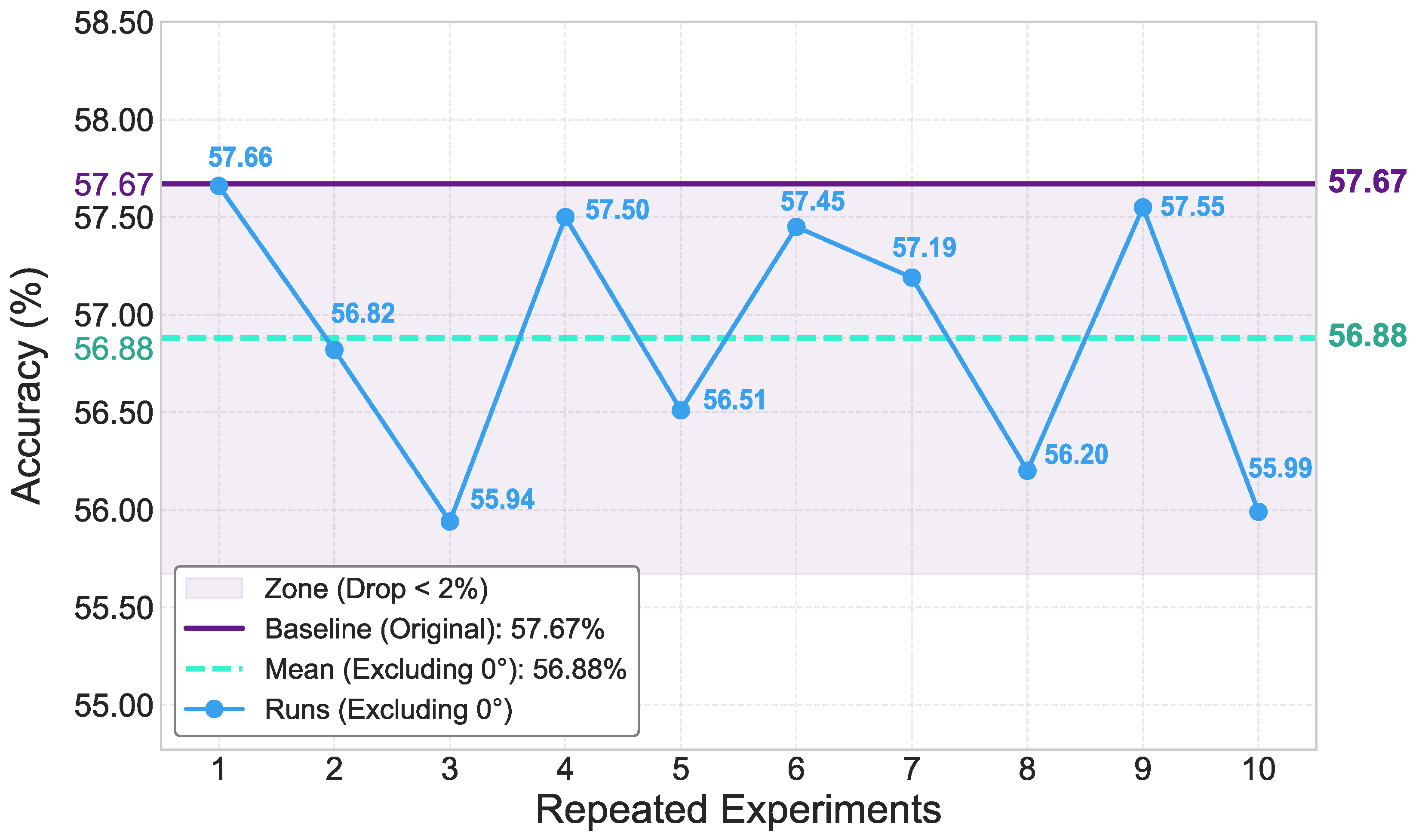
We designed an experiment to exclude samples from the training set to investigate whether back-scattering symmetry poses a risk of data leakage. We calculated the mean classification accuracy over ten repeated experiments on the 180° split. As shown in Figure A2, the mean accuracy after excluding samples is 56.88%. Compared to the baseline (57.67%), the decrease in accuracy is only 0.79%, which falls within the 2% tolerance threshold. This result indicates that the model does not significantly rely on viewpoint symmetry for classification.
Figure A2.
Impact of excluding 0° samples on classification accuracy on the 180° split.
References
- Kechagias-Stamatis, O.; Aouf, N. Automatic Target Recognition on Synthetic Aperture Radar Imagery: A Survey. IEEE Aerospace and Electronic Systems Magazine 2021, 36, 56–81. [Google Scholar] [CrossRef]
- Obaideen, K.; McCafferty-Leroux, A.; Hilal, W.; AlShabi, M.; Gadsden, S.A. Analysis of deep learning in automatic target recognition: evolution and emerging trends. In Proceedings of the Automatic Target Recognition XXXV; Chen, K., Hammoud, R.I., Overman, T.L., Eds.; International Society for Optics and Photonics, SPIE, 2025; Vol. 13463, p. 134630E. [Google Scholar] [CrossRef]
- Chen, B.; Liu, H.; Chai, J.; Bao, Z. Large margin feature weighting method via linear programming. IEEE Transactions on Knowledge and Data Engineering 2008, 21, 1475–1488. [Google Scholar] [CrossRef]
- Fu, Z.; Li, S.; Li, X.; Dan, B.; Wang, X. A Neural Network with Convolutional Module and Residual Structure for Radar Target Recognition Based on High-Resolution Range Profile. Sensors 2020, 20. [Google Scholar] [CrossRef]
- Wang, J.; Liu, Z.; Xie, R.; Ran, L. Radar HRRP target recognition based on dynamic learning with limited training data. Remote Sensing 2021, 13, 750. [Google Scholar] [CrossRef]
- Jacobs, S.; O’Sullivan, J. Automatic target recognition using sequences of high resolution radar range-profiles. IEEE Transactions on Aerospace and Electronic Systems 2000, 36, 364–381. [Google Scholar] [CrossRef]
- Du, L.; Liu, H.; Bao, Z. Radar HRRP statistical recognition: Parametric model and model selection. IEEE Transactions on Signal Processing 2008, 56, 1931–1944. [Google Scholar] [CrossRef]
- Liao, X.; Runkle, P.; Carin, L. Identification of ground targets from sequential high-range-resolution radar signatures. IEEE Transactions on Aerospace and Electronic systems 2003, 38, 1230–1242. [Google Scholar] [CrossRef]
- Du, L.; Wang, P.; Liu, H.; Pan, M.; Chen, F.; Bao, Z. Bayesian Spatiotemporal Multitask Learning for Radar HRRP Target Recognition. IEEE Transactions on Signal Processing 2011, 59, 3182–3196. [Google Scholar] [CrossRef]
- Meng, Y.; Wang, L.; Zhou, Q.; Zhang, X.; Zhang, L.; Wang, Y. Sparse View HRRP Recognition Based on Dual-Task of Generation and Recognition Method. In Proceedings of the 2024 IEEE International Conference on Signal, Information and Data Processing (ICSIDP); 2024; pp. 1–5. [Google Scholar] [CrossRef]
- Zhou, Q.; Yu, B.; Wang, Y.; Zhang, L.; Zheng, L.; Zou, D.; Zhang, X. Generative Multi-View HRRP Recognition Based on Cascade Generation and Fusion Network. In Proceedings of the 2024 International Radar Conference (RADAR), 2024; pp. 1–5. [Google Scholar] [CrossRef]
- Li, X.; Ouyang, W.; Pan, M.; Lv, S.; Ma, Q. Continuous learning method of radar HRRP based on CVAE-GAN. IEEE Transactions on Geoscience and Remote Sensing 2023, 61, 1–19. [Google Scholar] [CrossRef]
- Feng, B.; Chen, B.; Liu, H. Radar HRRP target recognition with deep networks. Pattern Recognition 2017, 61, 379–393. [Google Scholar] [CrossRef]
- Yin, H.; Guo, Z. Radar HRRP target recognition with one-dimensional CNN. Telecommun. Eng 2018, 58, 1121–1126. [Google Scholar]
- Xu, B.; Chen, B.; Wan, J.; Liu, H.; Jin, L. Target-Aware Recurrent Attentional Network for Radar HRRP Target Recognition. Signal Processing 2019, 155, 268–280. [Google Scholar] [CrossRef]
- Liu, J.; Chen, B.; Chen, W.; Yang, Y. Radar HRRP Target Recognition with Target Aware Two-Dimensional Recurrent Neural Network. In Proceedings of the 2019 IEEE International Conference on Signal Processing, Communications and Computing (ICSPCC), 2019; pp. 1–6. [Google Scholar] [CrossRef]
- Hochreiter, S.; Schmidhuber, J. Long Short-Term Memory. Neural Computation 1997, 9, 1735–1780. Available online: https://direct.mit.edu/neco/article-pdf/9/8/1735/813796/neco.1997.9.8.1735.pdf. [CrossRef] [PubMed]
- Cho, K.; Van Merriënboer, B.; Gulcehre, C.; Bahdanau, D.; Bougares, F.; Schwenk, H.; Bengio, Y. Learning phrase representations using RNN encoder-decoder for statistical machine translation. arXiv 2014, arXiv:1406.1078. [Google Scholar] [CrossRef]
- Pascanu, R.; Mikolov, T.; Bengio, Y. On the difficulty of training recurrent neural networks. In Proceedings of the International conference on machine learning. Pmlr, 2013; pp. 1310–1318. [Google Scholar]
- Zhao, H.; Jiang, L.; Jia, J.; Torr, P.H.; Koltun, V. Point transformer. In Proceedings of the Proceedings of the IEEE/CVF international conference on computer vision, 2021; pp. 16259–16268. [Google Scholar]
- Zhang, L.; Han, C.; Wang, Y.; Li, Y.; Long, T. Polarimetric HRRP recognition based on feature-guided Transformer model. Electronics Letters 2021, 57, 705–707. [Google Scholar] [CrossRef]
- Diao, Y.; Liu, S.; Gao, X.; Liu, A. Position Embedding-Free Transformer for Radar HRRP Target Recognition. In Proceedings of the IGARSS 2022 - 2022 IEEE International Geoscience and Remote Sensing Symposium, 2022; pp. 1896–1899. [Google Scholar] [CrossRef]
- Gulati, A.; Qin, J.; Chiu, C.C.; Parmar, N.; Zhang, Y.; Yu, J.; Han, W.; Wang, S.; Zhang, Z.; Wu, Y.; et al. Conformer: Convolution-augmented Transformer for Speech Recognition. Interspeech 2020 2020. [Google Scholar]
- Gu, A.; Dao, T. Mamba: Linear-time sequence modeling with selective state spaces. In Proceedings of the First conference on language modeling; 2024. [Google Scholar]
- Wang, Z.; Kong, F.; Feng, S.; Wang, M.; Yang, X.; Zhao, H.; Wang, D.; Zhang, Y. Is mamba effective for time series forecasting? Neurocomputing 2025, 619, 129178. [Google Scholar] [CrossRef]
- Rajah, P.; Odindi, J.; Mutanga, O. Feature level image fusion of optical imagery and Synthetic Aperture Radar (SAR) for invasive alien plant species detection and mapping. Remote Sensing Applications: Society and Environment 2018, 10, 198–208. [Google Scholar] [CrossRef]
- Lin, Y.; Zhang, H.; Lin, H.; Gamba, P.E.; Liu, X. Incorporating synthetic aperture radar and optical images to investigate the annual dynamics of anthropogenic impervious surface at large scale. Remote sensing of environment 2020, 242, 111757. [Google Scholar] [CrossRef]
- Chu, Z.; Luo, H.; Zhang, T.; Zhao, C.; Lin, B.; Gao, F. Micro-Doppler and HRRP Enabled UAV and Bird Recognition Scheme for ISAC System. In Proceedings of the 2025 IEEE/CIC International Conference on Communications in China (ICCC), 2025; pp. 1–6. [Google Scholar] [CrossRef]
- Yang, L.; Feng, W.; Wu, Y.; Huang, L.; Quan, Y. Radar-infrared sensor fusion based on hierarchical features mining. IEEE Signal Processing Letters 2023, 31, 66–70. [Google Scholar] [CrossRef]
- Zhang, F.; Bi, X.; Zhang, Z.; Xu, Y. HIFR-Net: A HRRP-Infrared Fusion Recognition Network Capable of Handling Modality Missing and Multisource Data Misalignment. IEEE Sensors Journal 2025, 25, 5769–5781. [Google Scholar] [CrossRef]
- Wang, Y.; Deng, J.; Li, Y.; Hu, J.; Liu, C.; Zhang, Y.; Ji, J.; Ouyang, W.; Zhang, Y. Bi-LRFusion: Bi-Directional LiDAR-Radar Fusion for 3D Dynamic Object Detection. In Proceedings of the Proceedings of the IEEE/CVF Conference on Computer Vision and Pattern Recognition (CVPR), June 2023; pp. 13394–13403. [Google Scholar]
- Xu, R.; Xiang, Z. RLNet: Adaptive Fusion of 4D Radar and Lidar for 3D Object Detection. In Proceedings of the Computer Vision – ECCV 2024 Workshops; Del Bue, A., Canton, C., Pont-Tuset, J., Tommasi, T., Eds.; Cham, 2025; pp. 181–194. [Google Scholar]
- Li, Y.; Ibanez-Guzman, J. Lidar for Autonomous Driving: The Principles, Challenges, and Trends for Automotive Lidar and Perception Systems. IEEE Signal Processing Magazine 2020, 37, 50–61. [Google Scholar] [CrossRef]
- Widdowson, D.; Kurlin, V. Recognizing rigid patterns of unlabeled point clouds by complete and continuous isometry invariants with no false negatives and no false positives. In Proceedings of the Proceedings of the IEEE/CVF Conference on Computer Vision and Pattern Recognition, 2023; pp. 1275–1284. [Google Scholar]
- Qi, C.R.; Su, H.; Mo, K.; Guibas, L.J. PointNet: Deep Learning on Point Sets for 3D Classification and Segmentation. In Proceedings of the Proceedings of the IEEE Conference on Computer Vision and Pattern Recognition (CVPR), July 2017. [Google Scholar]
- Qi, C.R.; Yi, L.; Su, H.; Guibas, L.J. Pointnet++: Deep hierarchical feature learning on point sets in a metric space. Advances in neural information processing systems 2017, 30. [Google Scholar]
- Guo, B.; Huang, X.; Zhang, F.; Sohn, G. Classification of airborne laser scanning data using JointBoost. ISPRS Journal of Photogrammetry and Remote Sensing 2015, 100, 71–83. [Google Scholar] [CrossRef]
- Liu, Z.; Tang, H.; Lin, Y.; Han, S. Point-voxel cnn for efficient 3d deep learning. Advances in neural information processing systems 2019, 32. [Google Scholar]
- Hsu, P.H.; Zhuang, Z.Y. Incorporating handcrafted features into deep learning for point cloud classification. Remote Sensing 2020, 12, 3713. [Google Scholar] [CrossRef]
- Wang, Y.; Sun, Y.; Liu, Z.; Sarma, S.E.; Bronstein, M.M.; Solomon, J.M. Dynamic Graph CNN for Learning on Point Clouds. In ACM Transactions on Graphics (TOG); 2019. [Google Scholar]
- Ma, X.; Qin, C.; You, H.; Ran, H.; Fu, Y. Rethinking network design and local geometry in point cloud: A simple residual MLP framework. arXiv 2022, arXiv:2202.07123. [Google Scholar] [CrossRef]
- Liang, D.; Zhou, X.; Xu, W.; Zhu, X.; Zou, Z.; Ye, X.; Tan, X.; Bai, X. Pointmamba: A simple state space model for point cloud analysis. Advances in neural information processing systems 2024, 37, 32653–32677. [Google Scholar]
- Baltrušaitis, T.; Ahuja, C.; Morency, L.P. Multimodal machine learning: A survey and taxonomy. IEEE transactions on pattern analysis and machine intelligence 2018, 41, 423–443. [Google Scholar] [CrossRef]
- Guo, W.; Wang, J.; Wang, S. Deep multimodal representation learning: A survey. Ieee Access 2019, 7, 63373–63394. [Google Scholar] [CrossRef]
- Boulahia, S.Y.; Amamra, A.; Madi, M.R.; Daikh, S. Early, intermediate and late fusion strategies for robust deep learning-based multimodal action recognition. Machine Vision and Applications 2021, 32, 121. [Google Scholar] [CrossRef]
- Dietz, S.; Altstidl, T.; Zanca, D.; Eskofier, B.; Nguyen, A. How Intermodal Interaction Affects the Performance of Deep Multimodal Fusion for Mixed-Type Time Series. In Proceedings of the 2024 International Joint Conference on Neural Networks (IJCNN), 2024; IEEE; pp. 1–8. [Google Scholar]
- Guarrasi, V.; Aksu, F.; Caruso, C.M.; Di Feola, F.; Rofena, A.; Ruffini, F.; Soda, P. A systematic review of intermediate fusion in multimodal deep learning for biomedical applications. Image and Vision Computing 2025, 105509. [Google Scholar] [CrossRef]
- Tan, H.; Bansal, M. Lxmert: Learning cross-modality encoder representations from transformers. arXiv 2019, arXiv:1908.07490. [Google Scholar] [CrossRef]
- Xu, K.; Ba, J.; Kiros, R.; Cho, K.; Courville, A.; Salakhudinov, R.; Zemel, R.; Bengio, Y. Show, attend and tell: Neural image caption generation with visual attention. In Proceedings of the International conference on machine learning. PMLR, 2015; pp. 2048–2057. [Google Scholar]
- Katharopoulos, A.; Vyas, A.; Pappas, N.; Fleuret, F. Transformers are RNNs: Fast Autoregressive Transformers with Linear Attention. In Proceedings of the Proceedings of the 37th International Conference on Machine Learning; III, H.D.; Singh, A., Eds. PMLR, 13–18 Jul 2020, Vol. 119, Proceedings of Machine Learning Research; pp. 5156–5165.
- Shen, Z.; Zhang, M.; Zhao, H.; Yi, S.; Li, H. Efficient Attention: Attention With Linear Complexities. In Proceedings of the Proceedings of the IEEE/CVF Winter Conference on Applications of Computer Vision (WACV), January 2021; pp. 3531–3539. [Google Scholar]
- Zhu, L.; Liao, B.; Zhang, Q.; Wang, X.; Liu, W.; Wang, X. Vision mamba: efficient visual representation learning with bidirectional state space model. In Proceedings of the Proceedings of the 41st International Conference on Machine Learning. JMLR.org, 2024; p. ICML’24. [Google Scholar]
- Chen, J.; Xu, S.; Chen, Z. Convolutional neural network for classifying space target of the same shape by using RCS time series. IET Radar, Sonar & Navigation 2018, 12, 1268–1275. [Google Scholar] [CrossRef]
- Zhang, Y.P.; Zhang, Q.; Kang, L.; Luo, Y.; Zhang, L. End-to-end recognition of similar space cone–cylinder targets based on complex-valued coordinate attention networks. IEEE Transactions on Geoscience and Remote Sensing 2021, 60, 1–14. [Google Scholar] [CrossRef]
- Ertin, E.; Austin, C.D.; Sharma, S.; Moses, R.L.; Potter, L.C. GOTCHA experience report: three-dimensional SAR imaging with complete circular apertures. In Proceedings of the Algorithms for Synthetic Aperture Radar Imagery XIV; Zelnio, E.G., Garber, F.D., Eds.; International Society for Optics and Photonics, SPIE, 2007; Vol. 6568, p. 656802. [Google Scholar] [CrossRef]
- TREATY, N.A. Target Identification and Recognition using RF Systems.
- Geffrin, J.M.; Sabouroux, P.; Eyraud, C. Free space experimental scattering database continuation: Experimental set-up and measurement precision. inverse Problems 2005, 21, S117. [Google Scholar] [CrossRef]
- Zhang, Y.P.; Zhang, L.; Kang, L.; Wang, H.; Luo, Y.; Zhang, Q. Space Target Classification With Corrupted HRRP Sequences Based on Temporal–Spatial Feature Aggregation Network. IEEE Transactions on Geoscience and Remote Sensing 2023, 61, 1–18. [Google Scholar] [CrossRef]
- Li, H.; Li, X.; Xu, Z.; Jin, X.; Su, F. MSDP-Net: A Multi-Scale Domain Perception Network for HRRP Target Recognition. Remote Sensing 2025, 17. [Google Scholar] [CrossRef]
- Vaswani, A.; Shazeer, N.; Parmar, N.; Uszkoreit, J.; Jones, L.; Gomez, A.N.; Kaiser, Ł.; Polosukhin, I. Attention is all you need. Advances in neural information processing systems 2017, 30. [Google Scholar]
Figure 1.
Complementarity of point clouds and HRRP. The top row shows that three distinct targets ((a) cone, (b) cylinder, (c) cone-cylinder) appear identical from the base view. In contrast, the bottom row (d–f) displays distinct HRRP.
Figure 1.
Complementarity of point clouds and HRRP. The top row shows that three distinct targets ((a) cone, (b) cylinder, (c) cone-cylinder) appear identical from the base view. In contrast, the bottom row (d–f) displays distinct HRRP.
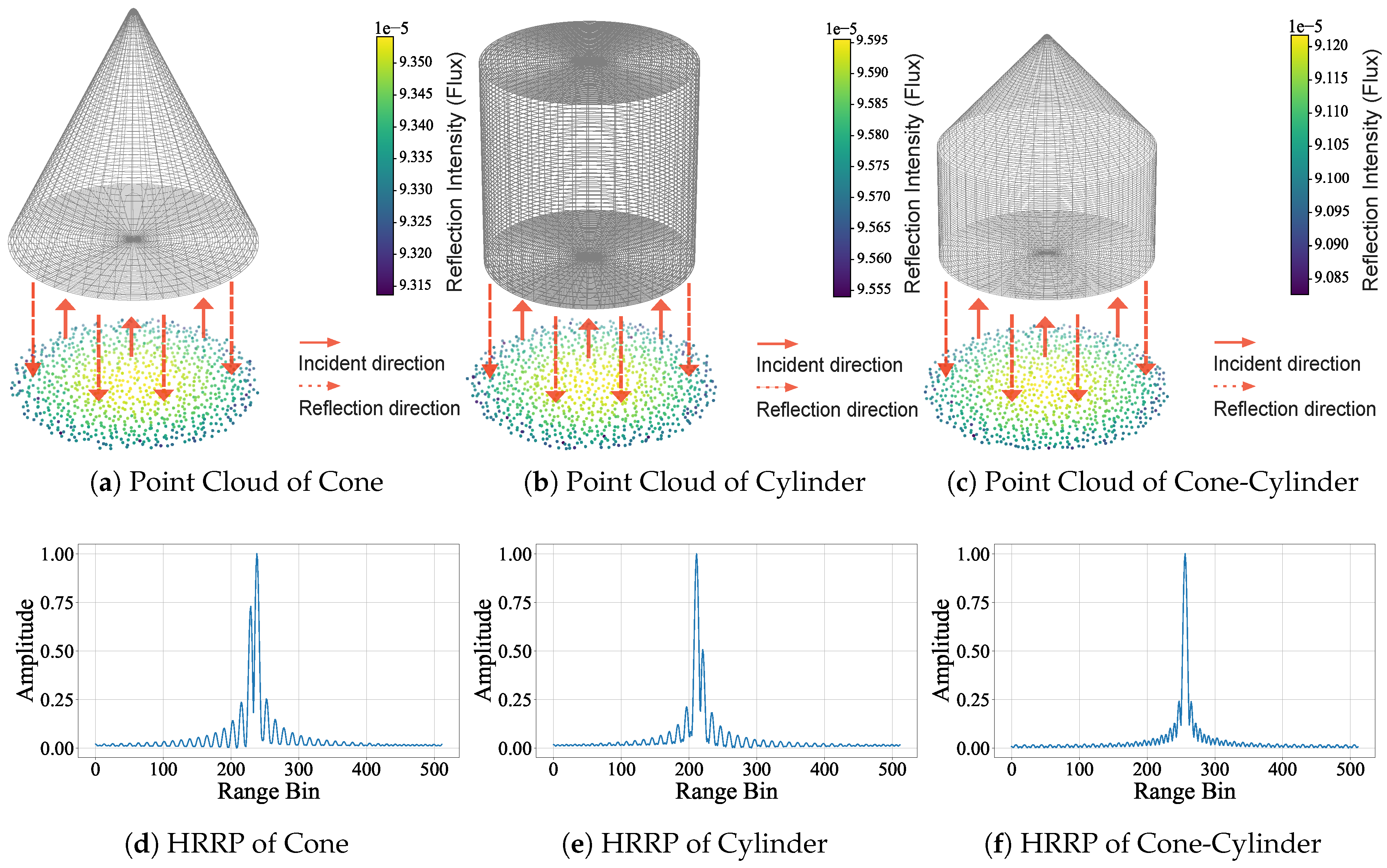
Figure 2.
Overview of Point-HRRP-Net. The framework operates in three stages: (1) Dual-branch Feature Extraction for HRRP and point clouds, (2) Cross-Attention Fusion via the Bi-CA mechanism, and (3) Classification. (HRRP: High Resolution Range Profile; PC: Point Cloud; FFT: Fast Fourier Transform; Bi-CA: Bi-Directional Cross-Attention; DGCNN: Dynamic Graph CNN).
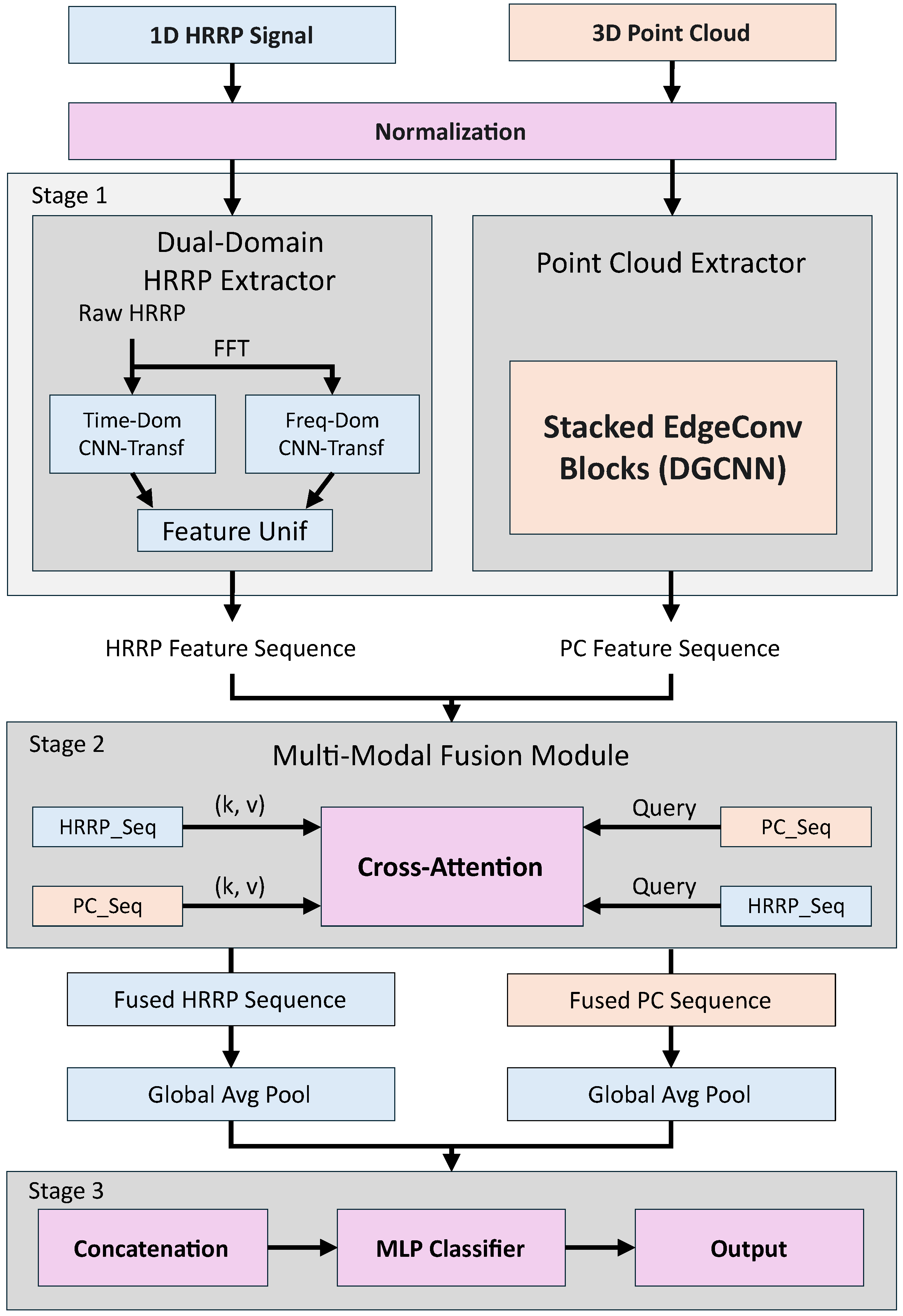
Figure 3.
Structure of the Dual-Domain HRRP Extractor. The module processes the raw HRRP and its amplitude spectrum in parallel. Each branch employs a 1D-CNN for local feature extraction and a Transformer Encoder for global dependency modeling. Finally, the features are projected and concatenated to form a unified HRRP feature sequence.
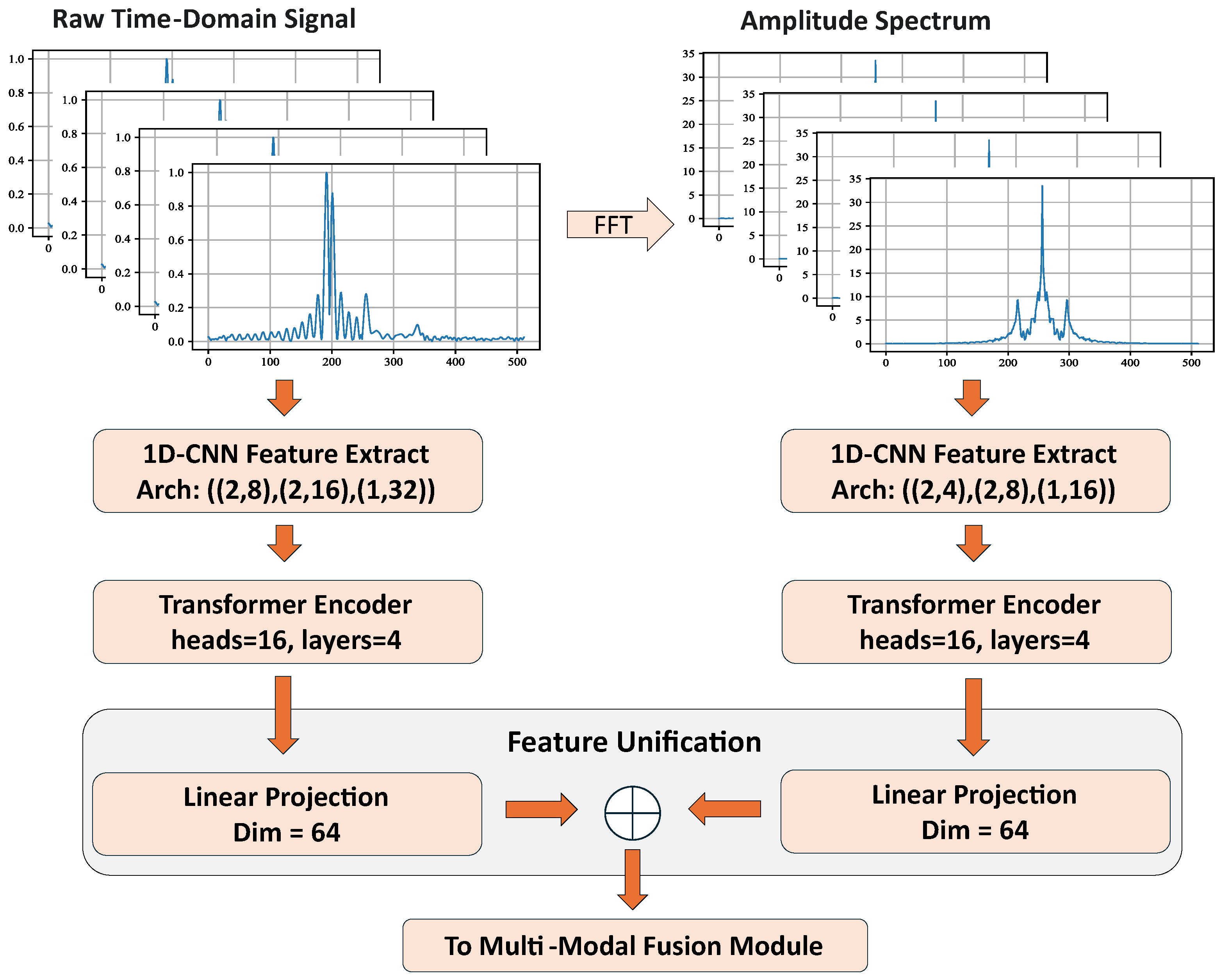
Figure 4.
Data flow of the time-domain 1D-CNN branch. The input tensor of shape traverses three stacked 1D-CNN blocks for local feature extraction and downsampling via Max-Pooling. Subsequently, a Transformer Encoder captures global dependencies to produce the final HRRP feature sequence.
Figure 4.
Data flow of the time-domain 1D-CNN branch. The input tensor of shape traverses three stacked 1D-CNN blocks for local feature extraction and downsampling via Max-Pooling. Subsequently, a Transformer Encoder captures global dependencies to produce the final HRRP feature sequence.
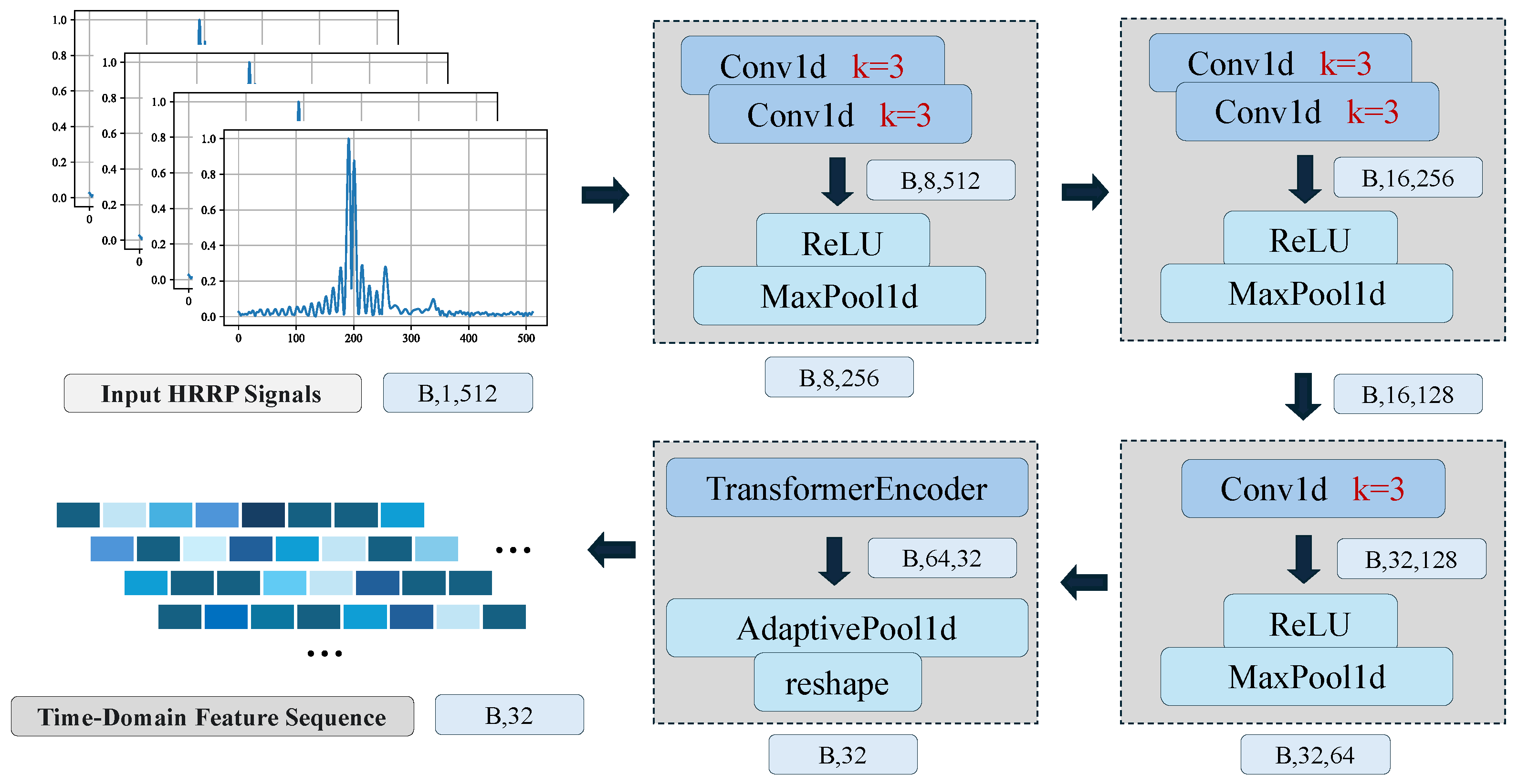
Figure 5.
Mechanism of the Cross-Attention module. The geometric query computes attention weights with electromagnetic keys . These weights aggregate the values to generate the enriched output .
Figure 5.
Mechanism of the Cross-Attention module. The geometric query computes attention weights with electromagnetic keys . These weights aggregate the values to generate the enriched output .
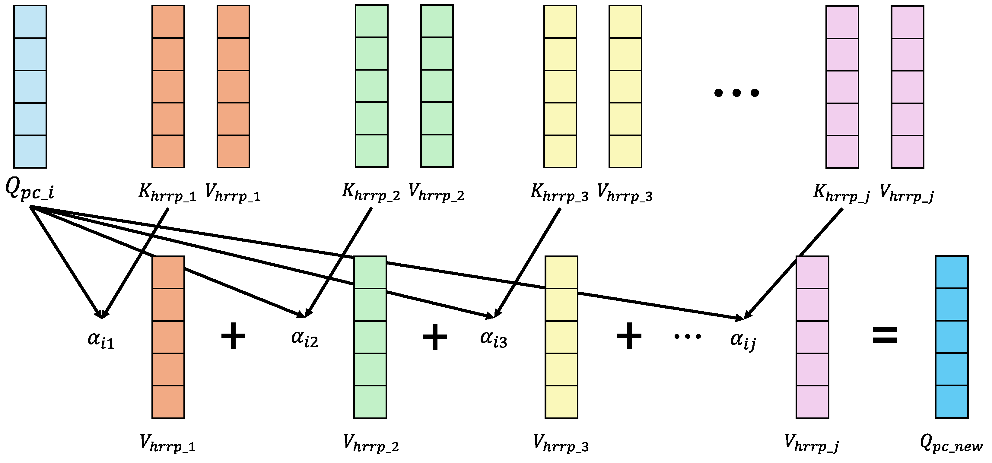
Figure 6.
Illustration of the simulation coordinate system and the definition of the incident angle . The angle represents the line-of-sight for both point cloud generation and electromagnetic simulations, shown here with the cylinder target.
Figure 6.
Illustration of the simulation coordinate system and the definition of the incident angle . The angle represents the line-of-sight for both point cloud generation and electromagnetic simulations, shown here with the cylinder target.
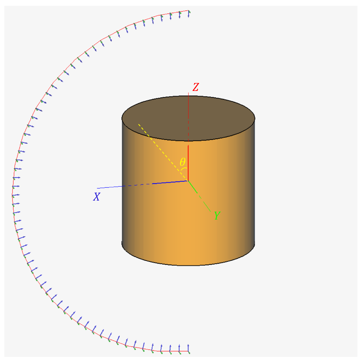
Figure 7.
Longitudinal cross-sections showing the dimensional parameters of the three simulated Perfect Electrical Conductor (PEC) targets. ((a) Cone, (b) Cylinder, and (c) Cone-cylinder composite. The points , , and denote the origin of each target’s local coordinate system. All dimensions are in meters. To ensure numerical stability during simulation, the sharp tips in (a) and (c) are replaced with small paraboloids, as detailed in the text.
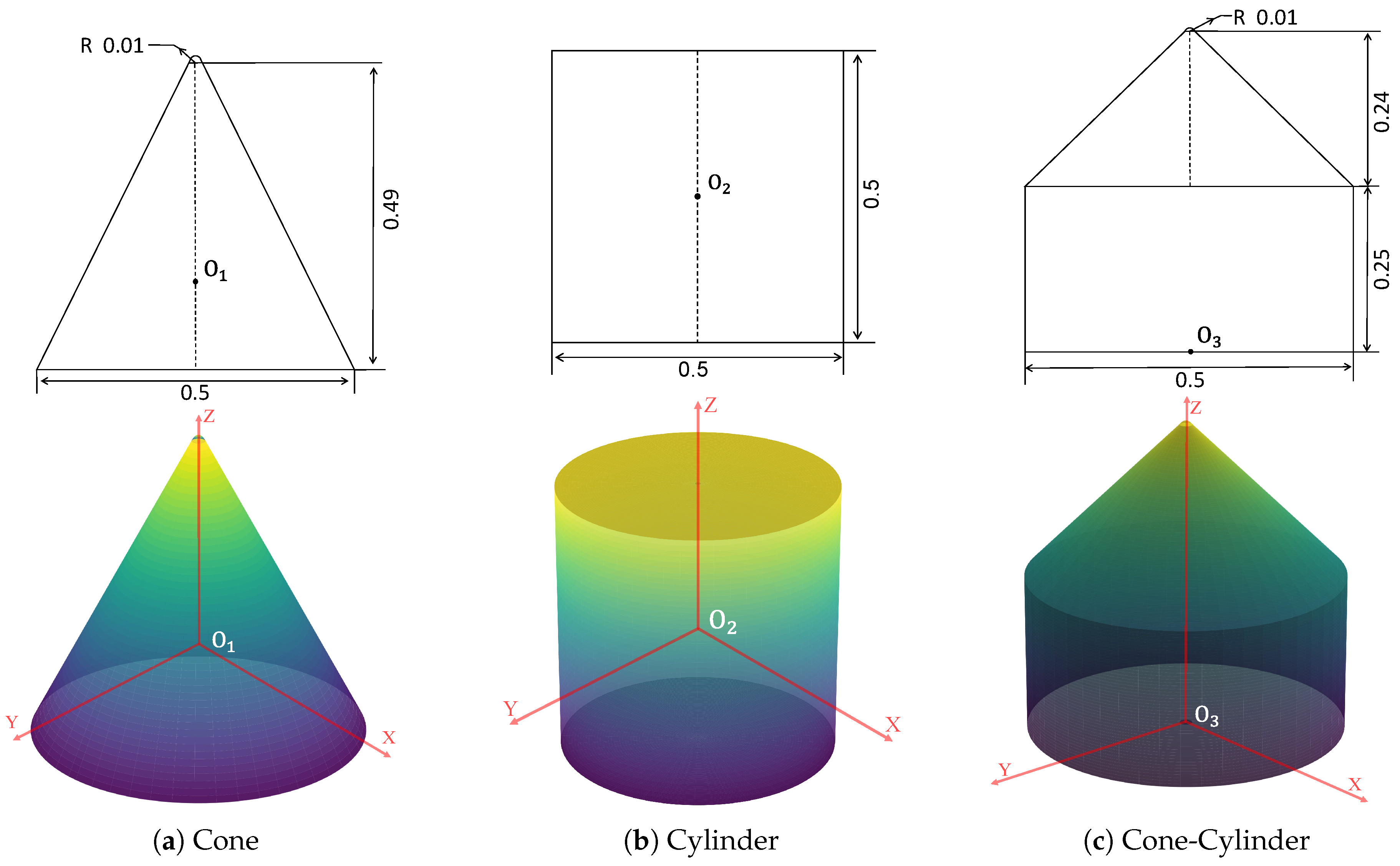
Figure 8.
Visualization of the attention weights in the Bi-CA module. (a, b) Attention distribution on the HRRP time-domain signal and frequency-domain spectrum, respectively, when queried by point cloud features. (c) Attention distribution on the 3D point cloud when queried by HRRP features. In the heatmaps, yellow regions denote higher attention weights (high relevance), whereas blue regions indicate lower weights.
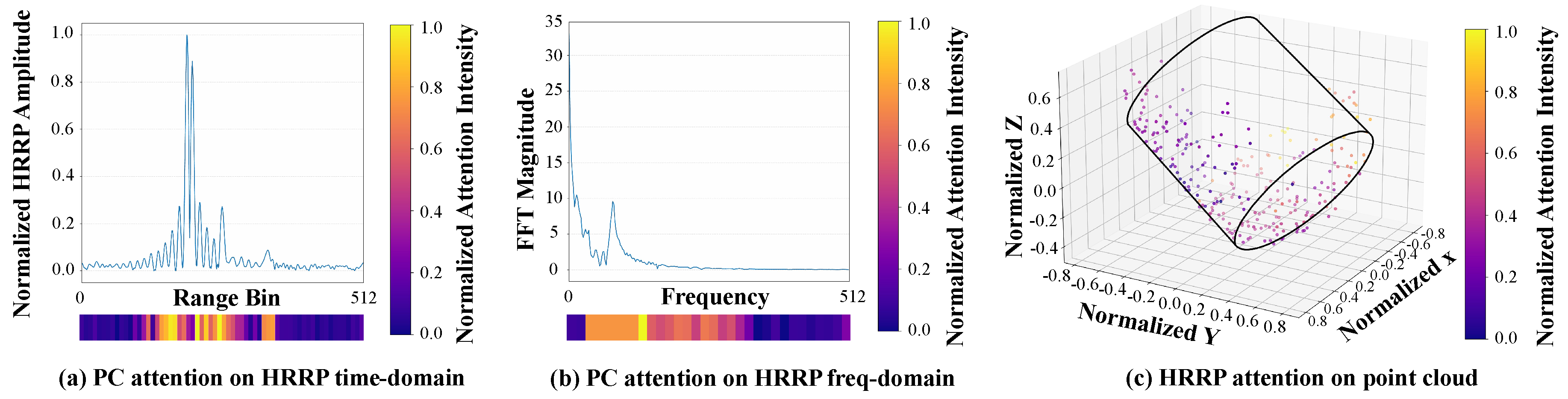
Figure 9.
Impact of Rotational Offset on Classification Accuracy ( Split). The solid green line represents the average accuracy, while the light green shaded area indicates the accuracy fluctuation range across test samples. The x-axis denotes the rotational offset () between the two modalities, and the y-axis represents the classification accuracy.
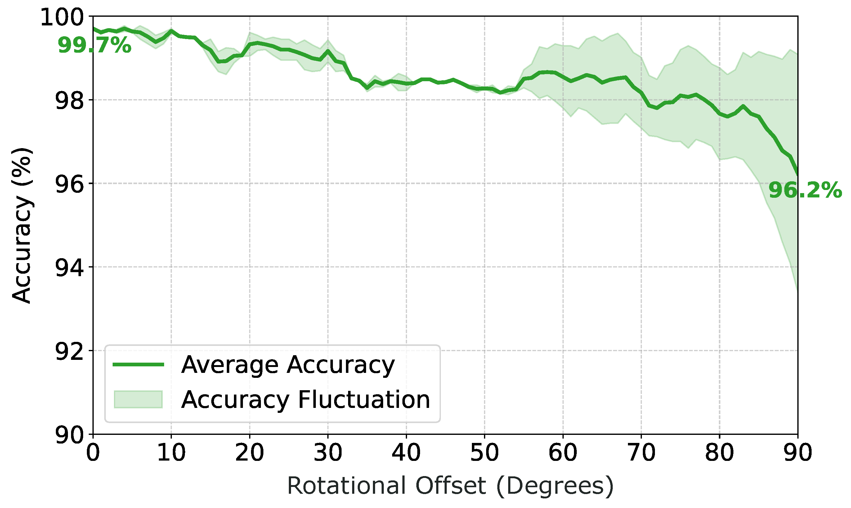
Figure 10.
Sensitivity Analysis of Rotational Offset Across Different Dataset Splits. The graph compares average accuracy trends for dataset splits ranging from to under increasing rotational offset.
Figure 10.
Sensitivity Analysis of Rotational Offset Across Different Dataset Splits. The graph compares average accuracy trends for dataset splits ranging from to under increasing rotational offset.
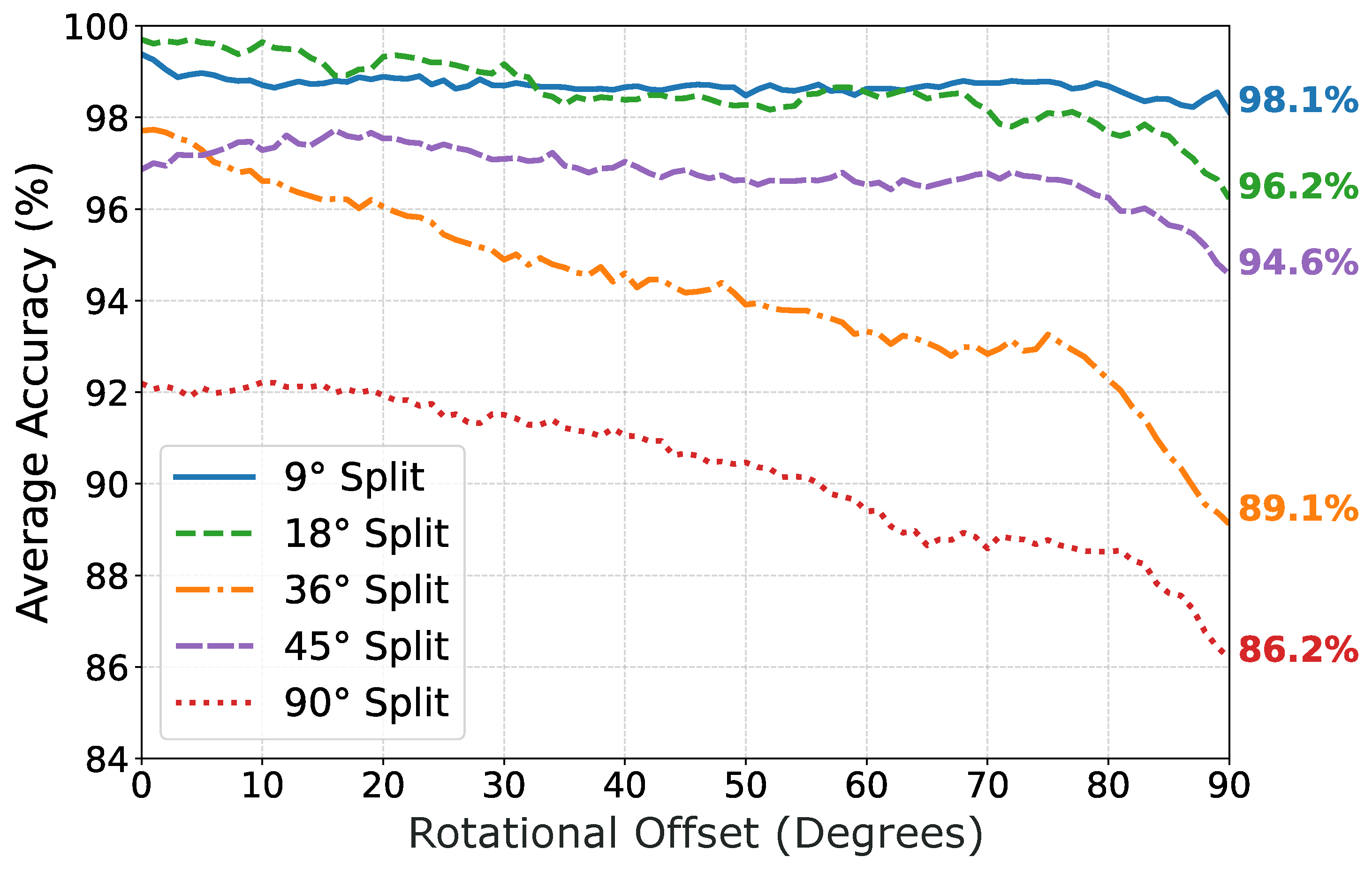
Figure 11.
Performance Degradation under Progressive Stress Tests. The x-axis represents degradation severity across three metrics: HRRP SNR (dB), Point Cloud Jitter (), and Point Cloud Drop rate (%). The curves illustrate the average accuracy of the model trained on the split under four test scenarios: HRRP noise only, PC jitter only, PC point drop only, and the aggregate of all three.
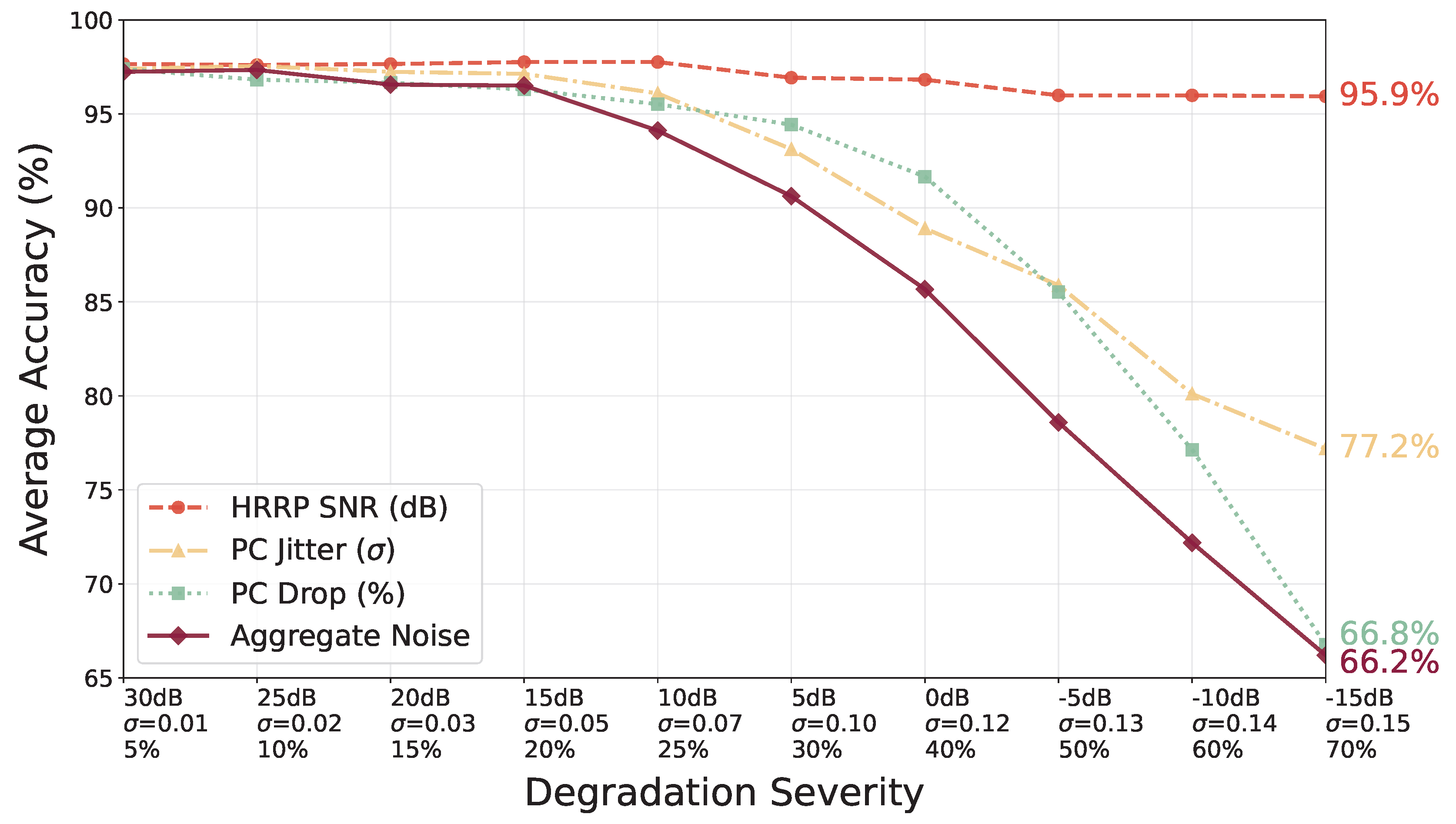
Table 1.
Generalization Performance Comparison against Representative Single-Modality Methods.
| Model | Modality | 9° Split | 18° Split | 36° Split | 45° Split | 90° Split | 180° Split |
|---|---|---|---|---|---|---|---|
| Ours (HRRP-only) | HRRP | 54.22 | 60.26 | 56.15 | 54.22 | 49.74 | 45.62 |
| 1D-Mamba [25] | HRRP | 65.05 | 60.78 | 58.49 | 60.16 | 51.35 | 42.34 |
| Conformer [23] | HRRP | 74.43 | 75.00 | 68.54 | 61.93 | 47.45 | 52.45 |
| MSDP-Net [59] | HRRP | 73.70 | 71.56 | 67.66 | 69.48 | 49.48 | 43.96 |
| Point-Transformer [20] | Point Cloud | 83.12 | 77.50 | 67.55 | 71.82 | 39.79 | 37.81 |
| DGCNN [40] | Point Cloud | 89.74 | 90.16 | 82.92 | 76.25 | 51.77 | 41.56 |
| PointMLP [41] | Point Cloud | 79.84 | 70.52 | 71.41 | 66.93 | 46.88 | 42.97 |
| PointMamba [42] | Point Cloud | 93.33 | 91.51 | 81.93 | 79.90 | 60.57 | 53.80 |
| Point-HRRP-Net (Ours) | Point Cloud + HRRP | 97.51 | 93.84 | 85.57 | 87.29 | 66.34 | 57.67 |
Table 2.
Ablation Study on Fusion Strategies.
| Fusion Strategy | Params (M) | 9° Split (F1) | 45° Split (F1) | 90° Split (F1) | Latency (ms) | FLOPs (G) |
|---|---|---|---|---|---|---|
| Concatenation | 0.8271 | 93.12 | 80.83 | 51.77 | 5.9959 | 0.6273 |
| Addition | 0.7942 | 94.06 | 83.44 | 60.26 | 5.3409 | 0.6272 |
| Product | 0.7942 | 95.83 | 82.40 | 54.69 | 5.3470 | 0.6272 |
| Gating | 0.8436 | 95.73 | 81.77 | 58.44 | 5.9708 | 0.6273 |
| Self-Attention [60] | 0.8271 | 95.94 | 84.17 | 47.81 | 6.9912 | 0.6273 |
| Linear-Attention [50] | 0.9277 | 93.91 | 81.72 | 53.70 | 8.0915 | 0.6448 |
| Efficient-Attention [51] | 0.9277 | 91.72 | 84.58 | 48.54 | 7.6187 | 0.6448 |
| Bi-Mamba [52] | 0.8275 | 95.68 | 82.29 | 46.09 | 8.5317 | 0.6275 |
| Bi-CA (Ours) | 1.0272 | 97.47 | 85.09 | 65.54 | 8.7573 | 0.6624 |
Table 3.
Comprehensive Ablation Study on Feature Extractors. Each row represents a variation from our final model (last row), where one component is replaced to evaluate its contribution to the overall performance and efficiency.
Table 3.
Comprehensive Ablation Study on Feature Extractors. Each row represents a variation from our final model (last row), where one component is replaced to evaluate its contribution to the overall performance and efficiency.
| HRRP Extractor | PC Extractor | Params (M) | FLOPs (G) | 9° Split (F1) | 45° Split (F1) | 90° Split (F1) | Latency (ms) |
|---|---|---|---|---|---|---|---|
| CNN | DGCNN | 1.0272 | 0.6570 | 96.51 | 85.36 | 46.77 | 6.7711 |
| RNN | DGCNN | 1.1203 | 0.7194 | 85.31 | 66.15 | 49.06 | 7.1118 |
| LSTM [17] | DGCNN | 1.3705 | 0.7683 | 92.40 | 74.38 | 56.77 | 7.2894 |
| GRU [18] | DGCNN | 1.5002 | 0.8020 | 95.00 | 79.58 | 46.51 | 6.7926 |
| 1D-Mamba [25] | DGCNN | 1.0247 | 0.7072 | 96.56 | 74.32 | 50.10 | 6.5243 |
| Conformer [23] | DGCNN | 1.1850 | 0.7888 | 95.89 | 83.13 | 58.02 | 7.5473 |
| CNN-Transformer | PointNet [35] | 0.6191 | 0.0950 | 92.81 | 82.19 | 47.60 | 9.0498 |
| CNN-Transformer | PointNet++ [36] | 0.5733 | 1.2934 | 88.70 | 80.10 | 48.02 | 113.3443 |
| CNN-Transformer | PointMLP [41] | 1.6522 | 0.4754 | 84.53 | 73.65 | 54.90 | 14.7948 |
| CNN-Transformer | PointMamba [42] | 0.5422 | 0.0871 | 91.87 | 83.54 | 57.19 | 13.8087 |
| CNN-Transformer (Ours) | DGCNN (Ours) | 1.0272 | 0.6624 | 97.47 | 85.09 | 65.54 | 8.7573 |
Disclaimer/Publisher’s Note: The statements, opinions and data contained in all publications are solely those of the individual author(s) and contributor(s) and not of MDPI and/or the editor(s). MDPI and/or the editor(s) disclaim responsibility for any injury to people or property resulting from any ideas, methods, instructions or products referred to in the content. |
© 2026 by the authors. Licensee MDPI, Basel, Switzerland. This article is an open access article distributed under the terms and conditions of the Creative Commons Attribution (CC BY) license (http://creativecommons.org/licenses/by/4.0/).
Copyright: This open access article is published under a Creative Commons CC BY 4.0 license, which permit the free download, distribution, and reuse, provided that the author and preprint are cited in any reuse.


