
Submitted:
09 January 2026
Posted:
12 January 2026
You are already at the latest version
Abstract
Visual–inertial attitude estimation systems often suffer from accuracy degradation and instability when visual measurements are intermittently lost due to occlusion or illumination changes. To address this issue, this paper proposes an LSTM-EKF framework for dynamic attitude estimation under visual information loss. In the proposed method, an LSTM-based vision prediction network is designed to learn the temporal evolution of visual attitude measurements and to provide reliable pseudo-observations when camera data are unavailable, thereby maintaining continuous EKF updates. The algorithm is validated through turntable experiments, including long-term reciprocating rotation tests, continuous visual occlusion scanning experiments, and attitude accuracy evaluation experiments over an extended angular range. Experimental results show that the proposed LSTM-EKF effectively suppresses IMU error accumulation during visual outages and achieves lower RMSE compared with conventional EKF and AKF methods. In particular, the LSTM-EKF maintains stable estimation performance under a certain degree of visual occlusion and extends the effective attitude measurement range beyond the camera’s observable limits. These results demonstrate that the proposed method improves robustness and accuracy of visual–inertial attitude estimation in environments with intermittent visual degradation.
Keywords:
attitude measurement
; extended Kalman filter
; long short-term memory
; visual occlusion
; sensor fusion
1. Introduction
Accurate and continuous six-degree-of-freedom pose measurement has been widely recognized as one of the keys enabling technologies in intelligent manufacturing, industrial robot calibration, and autonomous driving. Among them, the accuracy of attitude measurement, which involves three rotational degrees of freedom, directly affects the precision of overall pose estimation. Since single-sensor-based schemes are susceptible to environmental disturbances and inherently limited in terms of measurement accuracy and long-term stability, multi-sensor data fusion–based attitude measurement methods have emerged as an effective solution for enhancing system robustness and measurement accuracy [1].
To improve attitude measurement accuracy, Sun et al. proposed a dual-IMU/vision integrated attitude estimation algorithm for mobile platforms, achieving fast and accurate relative attitude estimation [2]. Yan et al. developed a laser-tracking-based attitude measurement method that combines a two-dimensional position-sensitive detector with a monocular vision system [3]. Xiong et al. enhanced the accuracy of vision/IMU fusion algorithms by incorporating a real-time calibration–based multi-factor influence analysis framework together with an AEKF [4]. Overall, compared with single-sensor-based approaches, these multi-sensor fusion methods significantly improve attitude measurement accuracy. However, when information sources are missing in the measurement system—particularly when high-precision sensors fail—the measurement performance deteriorates rapidly, leading to limited system robustness.
KF is one of the most widely used approaches for multi-sensor data fusion. Compared with the standard KF, the EKF exhibits superior nonlinear handling capability. Unlike AKF, EKF does not impose strict requirements on initial parameter settings, and compared with the UKF, it offers lower computational complexity and better real-time performance [5,6,7]. However, the loss of measurement information sources can have a more pronounced adverse impact on EKF-based estimation performance [8].
To address the limitations of conventional EKF, recent studies have explored the integration of neural networks and deep learning techniques with traditional filtering frameworks, aiming to mitigate performance degradation caused by missing or unreliable measurement information during continuous iterative estimation [9].
Recent data-driven approaches integrate neural networks with Kalman filtering to improve state estimation accuracy by learning motion characteristics. LSTM- or BP-based methods have been shown to reduce estimation errors and enhance robustness compared with conventional filters [10,11,12,13]. However, their practical application is often limited by high computational cost, sensitivity to motion changes, and strong dependence on training data, especially under sensor degradation or visual information loss. These limitations motivate the development of an efficient learning-assisted EKF framework capable of maintaining stable and accurate estimation during visual occlusion.
In summary, existing data-driven and hybrid learning-based methods have demonstrated the potential of neural networks in improving tracking accuracy. However, most of these approaches suffer from high computational complexity, limited adaptability to abrupt motion, and strong dependence on data and application scenarios. Motivated by these limitations, proposed a LSTM-EKF–based dynamic attitude measurement framework that integrates temporal prediction into the EKF measurement update process, enabling stable and accurate attitude estimation under prolonged visual occlusion. By using the variation of object attitude obtained from vision measurements as training samples, the proposed LSTM network provides relatively high-accuracy reference outputs when visual measurements are unavailable due to environmental disturbances. Consequently, stable and continuous dynamic attitude measurement of the target can be achieved, enhancing the stability and robustness of the attitude measurement system.
The main contributions of this article are summarized as follows:
- An LSTM-EKF-based dynamic attitude estimation algorithm is proposed to address the degradation of estimation accuracy caused by visual information loss. By integrating temporal prediction into the EKF framework, the proposed method enhances the stability and robustness of attitude estimation under vision-degraded conditions;
- A visual prediction LSTM network is designed to compensate for missing visual measurements, providing reliable pseudo-observations for the EKF when visual data are unavailable. This enables stable attitude estimation during a certain degree of visual occlusion and effectively extends the measurable angular range of the attitude measurement system;
- Extensive experimental validations are conducted on a precision turntable platform, including long-term reciprocating rotation experiments, visual occlusion scanning experiments, and ablation studies. The results demonstrate that the proposed LSTM-EKF approach achieves higher accuracy and stronger robustness than EKF and AKF methods, particularly under visual occlusion.
2. Principle of Dynamic Attitude Measurement
2.1. Attitude Measurement System Components
To ensure real-time performance of the measurement system, both the IMU and the vision sensor are connected to the host computer via wired communication. The IMU is rigidly mounted on the target object. The overall configuration of the IMU/vision-based attitude measurement system is illustrated in Figure 1.
In this system, the following coordinate systems are defined: The origin of the vision coordinate system () is located at the optical center of the vision, along the optical axis, the axis points forward, the axis is horizontally to the right, and the axis points vertically downward. The origin of the cooperative target coordinate system () is located at the center of cooperative target, the vertical direction of the axis points to the IMU, and its and axes are determined by the right-hand rule. The origin of the IMU coordinate system () is at the sensitive center of the IMU, and the , , and axes are parallel to the corresponding axes of the target coordinate system.
The camera coordinate system is defined as the global reference frame. The transformation matrix between the target coordinate system and the IMU coordinate system is obtained through a rotary stage-based dynamic calibration procedure.
As illustrated in Figure 2, data for the dynamic attitude measurement system are acquired by both the IMU and the camera. The target images captured by the camera are first subjected to preprocessing operations, including attitude estimation and time-axis alignment. Subsequently, the preprocessed attitude angle data are evaluated to determine whether the camera output is abnormal. When the camera-derived attitude angles are valid, an EKF is employed for state updating. In contrast, when the camera measurements are abnormal or unavailable, an LSTM–EKF fusion algorithm is activated to maintain stable system operation. The detailed implementation procedure is described as follows.
First, the EPnP [14] algorithm is used to solve the target’s attitude angles in the visual coordinate system, and then the results are transformed into the global coordinate system through a rotation matrix. The monocular camera captures an image of the target, and after processing, the pixel coordinates of the feature points on the target are obtained:
In the EPNP algorithm, the space point P can be represented as the weighted sum of four control points , , in the target coordinate system:.
where represents the coordinates of the target feature points in the target coordinate system, and is the number of target feature points. is the weight coefficient of the control point, satisfying , .
Similarly, from the invariance of the linear relation under the Euclidean transformation, the target feature points can also be expressed in the camera coordinate system as:
In the camera coordinate system, the point can be converted to the point in the camera coordinate system by the rotation matrix and the translation vector :
The image coordinates corresponding to the target feature points are ), and the camera is calibrated by Zhang Zhengyou’s plane calibration method, and the internal reference matrix is A, which can be obtained according to the perspective projection model:
Where is the projection depth of the feature point; , , and are the internal parameters of the camera.
From the above formulas and the correspondence between the four spatial points and the image points, a linear system of equations for the weight coefficient can be obtained. After solving the system of equations, the rotation matrix and the translation vector can be determined by minimizing the reprojection error, and the expression for the reprojection error is:
where and are the principal point coordinates of the camera. Convert to a 3×3 matrix:
Based on the relationship between the rotation matrix and the Euler angle, the target attitude angle can be expressed as:
Since the target is rigidly connected with the test object, the attitude angle of the test object in the camera coordinate system can be obtained by the above formula:
Secondly, the attitude angle under the IMU coordinate system is obtained by the quaternion method, which is converted to the global coordinate system.
The quaternion solution formula based on differential equations is used to calculate the angular velocity data collected by the IMU gyroscope. Assuming the quaternion , the angular velocity vector output by the IMU is , and its differential equation can be expressed as:
In order to solve this differential equation, the system employs the fourth-order Runge-Kutta method [15] for numerical integration. Then, normalization is performed to obtain :
Furthermore, the attitude quaternion is converted into a rotation matrix through the conversion relationship between the quaternion and the rotation matrix, and the conversion formula is as follows:
Then, according to the relationship between the target coordinate system, the inertial coordinate system and the camera coordinate system, the rotation matrix containing the attitude information is converted to the global coordinate system, which is expressed as:
Similarly, based on the relationship between the rotation matrix and the Euler angles, the IMU calculates the attitude angle :
In this way, the Camera and IMU measurement results can be transformed into attitude angles.
2.2. Algorithm Design By LSTM-enhanced Extended Kalman Filter
In the proposed dynamic attitude measurement system, the EKF serves as the core approach for multi-sensor data fusion. In this study, the IMU outputs are formulated as the system state vector , while the attitude angles estimated by the camera are defined as the observation vector . Based on these definitions, the attitude measurement system can be modeled as a nonlinear state-space system, which is expressed as follows:
Where represents the state quantity of the system at time , is the measured value of the system at time , and represent the state noise and measurement noise of the system at time , respectively. and . represents the control input vector. and represent the nonlinear state transition function and observation function.
EKF primarily includes two steps: prediction and update.
Prediction Step:
Where is the Jacobian matrix of the state transition function and is the process noise Jacobian matrix, specifically:
Update Step:
The Kalman Gain:
Where is the Jacobian matrix of the observation equation.
State Update:
Error Covariance Update:
Where is the identity matrix.
Since the LSTM network is a type of recurrent neural network with strong capability in modeling temporal sequences, it has been widely applied in fields such as target tracking, speech translation, and image caption generation. Compared with the conventional RNN, LSTM effectively alleviates the problems of vanishing gradients and exploding gradients during training. Moreover, by introducing three gating mechanisms—namely the forget gate, input gate, and output gate—LSTM is able to selectively retain and update long-term and short-term information. The architecture of the LSTM network is illustrated in Figure 3.
In Figure 3, and represent the output values of the forget gate, input gate, and output gate, respectively; represents the cell state, and represents the update and activation of the current cell state.
Among them, the forget gate is used to control the information to be forgotten from the memory . The formula is as follows:
Where is the sigmoid activation function, which can be defined as:
Equation (23) and the following equations appearing and represent the weight parameters; and represent the bias parameters.
The input gate determines how many inputs enter the current cell state:
Candidate memory provides an alternative input, which is converted to a value between −1 and 1 by a hyperbolic tangent function, calculated as follows:
The cell state can then be found by the following formula:
The output gate determine the output by obtaining the output of the unit:
Based on the above principles, the LSTM-EKF algorithm structure designed in this paper is shown in Figure 4:
Figure 4 illustrates the detailed update procedure of the EKF employed in this study, as well as the basic architecture of the LSTM network used for visual measurement prediction. As shown in the Figure 4, at the EKF update instants when visual information is available, the fused attitude angles are jointly determined by the measurements from the IMU and the camera. When the camera provides normal attitude measurements, a standard EKF update is performed to achieve attitude fusion between the IMU and visual data.
In the case of abnormal or missing visual outputs, the visual attitude variations over the previous time steps are fed into the LSTM network as an input sequence, where the value of is determined through simulation analysis. The LSTM network outputs the predicted visual attitude increment from the last valid visual measurement to the current time step. By adding this predicted increment to the previous visual attitude measurement, the predicted visual attitude at the current time step is obtained, which serves as the observation vector . This predicted observation is then incorporated into the EKF update, enabling continuous and stable attitude estimation even under visual measurement degradation.
Therefore, the system observation vector can be expressed as:
Where is the switching threshold.
By integrating the LSTM network with the EKF, continuous dynamic attitude measurement can be achieved even under abnormal or missing camera measurements. The proposed approach significantly enhances the stability and robustness of the IMU/camera-based attitude measurement system, and effectively maintains high estimation accuracy when the visual system is affected by adverse factors such as illumination variations and occlusions.
3. Training Parameter Settings and Simulation
3.1. Dataset Construction and Network Structure Design
In Section 2, the overall structure of the proposed algorithm is defined. Within the fusion framework, the accuracy of the camera serves as the primary factor affecting the performance of the measurement system. Consequently, during visual occlusion, the accuracy of the visual prediction network directly determines the algorithm’s reliability in this period. To enhance the prediction performance of the neural networks, this section focuses on designing the network architecture.
Considering the output frequency of the camera in the attitude dynamic measurement system, an excessively short input sequence length results in large prediction errors, whereas an overly long input sequence reduces the network’s responsiveness to changes in complex measurement environments. Therefore, we select an optimal input length within the range of 5-to-20-time steps. To determine the best configuration, time-series cross-validation with five folds is employed to evaluate the influence of different input lengths on network performance, as illustrated in Figure 5.
As shown in Figure 5, when the input sequence length increases from 5 to 10, both the RMSE and MAE of the network decrease steadily. However, beyond a length of 10, RMSE and MAE exhibit only slight fluctuations around a nearly constant value. Therefore, we select an input sequence length of 16, as it yields a relatively small loss index. Additionally, increasing the input sequence length significantly increases the algorithm’s training time, which is unfavorable for handling visual occlusion scenarios at the beginning of the measurement process.
The hyperparameters of the neural network are determined using a random search strategy. Specifically, the number of layers is selected from 1, 2, 3 and 4, and the number of cells is chosen from 32, 64, 128 and 256. The combination yielding the minimum RMSE is selected, as shown in Figure 6.
As illustrated in Figure 6, for the LSTM, the minimum RMSE of 0.128° is achieved when the network contains one LSTM layer with 64 hidden units. Consequently, the network adopt different architectural configurations, as depicted in Figure 7.
As shown in Figure 7, the LSTM incorporates a dropout layer following the LSTM layer. This dropout layer is introduced to mitigate overfitting during training on the sample set. Subsequently, a fully connected layer is employed to reduce the dimensionality of the extracted features, thereby lowering computational complexity and further alleviating overfitting. A ReLU activation function is then applied to enhance the network’s ability to model complex nonlinear relationships and to address the vanishing gradient problem. Finally, another fully connected layer is appended to match the output requirements.
The models were developed using MATLAB’s Neural Network Toolbox. The experiments were conducted on a system running Windows 11 with an AMD R9-7945HX CPU, an NVIDIA RTX 4060 GPU with 8 GB of video memory, and 16 GB of RAM. The networks were trained using the Adam optimizer, which adaptively updates the network parameters based on the first- and second-order moments of the gradients.
3.2. Performance Simulation Analysis of Fusion Algorithms
After determining the system structure, simulations are conducted to evaluate the performance of the proposed algorithm. The simulation conditions are summarized in Table 1.
The training of the neural networks in the LSTM-EKF algorithm plays a critical role in the overall system performance. Therefore, prior to initiating the simulation experiments, the network is trained using predefined parameters. The training parameters are summarized in Table 2.
After finalizing the algorithm structure and training the neural networks using the designated datasets, simulation experiments were conducted to evaluate the performance of the proposed LSTM-EKF algorithm. For comparison, the traditional AKF and standard KF algorithms were also implemented. The total simulation duration was set to 60 seconds. During this period, the target was assumed to undergo constant angular motion with a rotational velocity of 5°/s.
To simulate visual occlusion scenarios, camera outputs were artificially removed between 31 and 40 seconds, representing 10 consecutive missing vision outputs. The goal was to evaluate the robustness of the algorithm under camera failure. The simulation results are illustrated in Figure 8.
As illustrated in Figure 8 the IMU-only measurements exhibit significant cumulative errors over time due to sensor drift and noise. These errors can be effectively mitigated through the fusion of IMU and vision data. During periods of visual data loss, the accuracy of both the KF and AKF degrades considerably. The AKF also exhibits a noticeable lag in measurement, attributed to disruptions in the visual input that impair the adaptive adjustment of filter parameters, resulting in model inaccuracies. Nevertheless, the AKF is capable of gradually restoring accuracy once visual information becomes available again. In contrast, the proposed LSTM-EKF algorithm maintains superior estimation accuracy throughout the occlusion period. This improvement is attributed to its integrated visual prediction and residual correction mechanisms. Consequently, the LSTM-EKF demonstrates high-precision measurement capability and effectively suppresses error divergence in the presence of visual occlusion, thereby enhancing the robustness and reliability of the measurement system.
4. Experiment
4.1. Experimental Platform
As illustrated in Figure 9, a precision two-dimensional turntable was employed to construct the experimental platform for validating the performance of the proposed dynamic attitude measurement algorithm.
In Figure 9, the IMU used in the experiment is the ADIS16488, a 10-degree-of-freedom sensor rigidly mounted on a fixed position of the cooperating target. The vision sensor utilized is the Basler acA2500-20gm, offering a resolution of 2590 × 2048 pixels.
4.2. Design of Experiments
To evaluate the performance of the proposed LSTM-EKF algorithm, two experiments were conducted: (1) a long-term reciprocating rotation experiment, and (2) an attitude accuracy evaluation experiment. The goal of the long-term reciprocating rotation experiment is to verify that the LSTM-EKF algorithm can effectively suppress the divergence of IMU cumulative errors during extended measurements. In addition, by comparing with conventional AKF and KF algorithms, this test demonstrates the proposed algorithm’s ability to accurately track target attitude even under visual occlusion.
The attitude accuracy evaluation experiment assesses the angular measurement accuracy at various rotation angles. It aims to validate that, compared with the AKF algorithm, the LSTM-EKF algorithm maintains high accuracy even when the rotation exceeds the vision sensor’s measurement range.
Prior to the experiments, the total station and vision sensor were rigidly mounted at fixed positions, and the cooperative target was secured to the turntable. The IMU was installed inside the target. Subsequently, calibration was performed for both the IMU error model and the intrinsic parameters of the vision sensor. The rotation matrices between all relevant coordinate systems were determined to establish their spatial relationships. The IMU sampling frequency was set to 100 Hz, and the vision sensor was configured to sample at 1 Hz.
The experimental procedures are as follows:
- Long-Term Reciprocating Rotation Experiment:
The turntable was configured to rotate back and forth over a ±50° range. The measurement system was activated, and the turntable executed multiple reciprocating rotations. During the experiment, the vision sensor was intermittently occluded for various durations to simulate visual missing. Upon completion of the predefined number of rotations, the turntable was stopped and stabilized before terminating the measurement.
- 2.
- Camera Occlusion Scanning Experiment:
Ten sets of repeated experiments were conducted for Occlusion Scanning. All algorithms were first evaluated using unobstructed data to obtain the benchmark RMSE. Subsequently, visual occlusion segments with frame lengths ranging from 1 to 30 were introduced at identical time points across all experimental runs. The RMSE of each algorithm with respect to the ground truth was then calculated, and the experimental results were recorded for further analysis.
- 3.
- Attitude Accuracy Evaluation Experiment:
The turntable was programmed to perform a single rotation from 0° to 80°, with measurements taken at every 5° interval. For each angle, repeated measurements were conducted. After the system initialization, the turntable was rotated to the specified angle, and the system recorded the results after stabilization was achieved.
4.3. Experimental Results and Analysis
- Long-Term Reciprocating Rotation Experiment:
The experimental results of the long-term reciprocating rotation experiment are illustrated in Figure 10.
As shown in Figure 10, the shaded regions indicate periods of visual signal loss. The visual output is categorized into measured and predicted values, which are clearly distinguished in the figure. During the occlusion periods, the missing visual data are reconstructed using the LSTM. From left to right, the number of missing visual frames is 5, 10, and 20, respectively.
It is evident that the standalone IMU exhibits significant cumulative errors over prolonged measurements. However, the proposed LSTM-EKF algorithm effectively corrects the IMU drift, significantly enhancing the measurement accuracy. Notably, even during visual occlusion, the LSTM-EKF algorithm maintains reliable attitude tracking and measurement performance.
To further evaluate the robustness of the algorithm, the LSTM-EKF is compared with the traditional AKF and KF algorithms under varying durations of visual occlusion. The comparative results are presented in Figure 11.
As illustrated in Figure 11, the LSTM-EKF algorithm consistently exhibits lower attitude estimation errors than the AKF and KF methods during periods of visual data loss. In Figure 11(a) and 11(b), it is evident that the errors associated with the AKF and KF algorithms progressively increase once the visual input is unavailable. In contrast, the LSTM-EKF maintains stable performance by adaptively correcting the IMU drift during the occlusion interval through its LSTM.
When the duration of visual occlusion becomes prolonged, as shown in Figure 11(c), the performance of the AKF and KF methods deteriorates significantly. Specifically, once the visual loss exceeds 10 seconds, their errors rapidly diverge. However, the proposed LSTM-EKF algorithm effectively suppresses this error divergence by leveraging the visual prediction and residual adaptively correcting mechanism, thereby maintaining a high level of measurement accuracy even in extended occlusion scenarios.
To comprehensively evaluate the performance of the three fusion algorithms, we compare both their overall measurement performance and their performance during visual occlusion. The comparison results are summarized in Table 3.
As shown in Table 3, the LSTM-EKF algorithm achieves the lowest RMSE and ME across the entire measurement duration compared with both AKF and KF, demonstrating superior accuracy and long-term stability. Although KF slightly outperforms AKF due to the constant rotational motion of the turntable, LSTM-EKF still improves the MAE by 19% and reduces the RMSE and ME by approximately 29% relative to KF.
During the visual occlusion periods, the estimation errors of both AKF and KF increase significantly, while the LSTM-EKF maintains consistent accuracy. Compared with AKF—which exhibits lower errors among traditional methods—LSTM-EKF achieves an 85% reduction in ME and approximately 59% reductions in both RMSE and MAE. This performance gain is attributed to the LSTM’s ability to accurately predict during vision loss. Moreover, the MAE and RMSE during occlusion remain close to those over the full sequence, confirming the algorithm’s robustness. These results indicate that the proposed LSTM-EKF algorithm provides accurate and reliable attitude estimation, especially under challenging conditions such as extended visual occlusion.
- 2.
- Camera Occlusion Scanning Experiment:
To evaluate the maximum effective prediction duration of the proposed LSTM network, a visual-missing duration scanning experiment was conducted. Ten long-duration oscillation experiments were performed with the same visual occlusion onset time. Under different visual missing durations, the RMSE of the IMU-only, KF, AKF, and LSTM-EKF methods were systematically compared. The experimental results are presented in Figure 12.
As shown in Figure 12, the estimation accuracy of all compared methods generally degrades as the number of consecutively missing camera frames increases. Nevertheless, among all fusion strategies, the LSTM-EKF method consistently achieves the highest estimation accuracy under different visual missing durations.
When the camera measurements are missing for 1–10 consecutive frames, both the LSTM-EKF and AKF approaches exhibit significantly lower RMSEs than the conventional KF. This improvement can be attributed to the adaptive mechanism of AKF, which is capable of adjusting model and noise parameters within a short time interval to suppress error divergence. However, when the number of consecutively missing frames exceeds 10, the RMSE of AKF also begins to diverge, showing a trend similar to that of the KF.
In contrast, the LSTM-EKF method exploits the LSTM network to predict the camera outputs and provides effective pseudo-measurements to the EKF during visual outages, thereby compensating for missing measurement updates and extending the duration over which RMSE divergence is suppressed. When the number of missing frames exceeds 20, the RMSE of the LSTM-EKF method also starts to diverge. These results indicate that, within 20 consecutive missing camera frames, the proposed LSTM-EKF approach can more effectively correct the accumulated IMU errors and maintain stable EKF updates compared with the KF and AKF methods.
- 3.
- Attitude Accuracy Evaluation Experiment:
Since the effective measurement range of the vision sensor is limited to 55°, visual measurements fail when the turntable rotation angle exceeds this range. The proposed LSTM-EKF algorithm leverages neural network predictions to estimate angles beyond this visual range, thereby effectively extending the measurement capability of the system. To evaluate this, an angular accuracy evaluation experiment was designed with turntable rotation angles ranging from 0° to 80°, in 5° increments, with multiple repeated measurements conducted for each group. As a representative example, the measurement results for an 80° rotation are illustrated in Figure 13.
In Figure 13, two types of colored markers indicate the visual measurement output and the predictions from the LSTM. The total measurement duration was approximately 21 seconds during the 80° rotation. Over this period, the IMU accumulated an error of approximately 1.3°, which continued to diverge over time. However, the errors associated with the LSTM-EKF, AKF, and KF algorithms were significantly smaller, indicating effective suppression of IMU error drift.
When the rotation angle exceeds 55°, the cooperative target moves out of the vision sensor’s observable range. During this visual loss phase, the LSTM-EKF algorithm employs its LSTM to continue correcting the system’s outputs based on learned motion patterns, thereby maintaining high measurement accuracy. The quantitative evaluation results of angular measurement accuracy are summarized in Table 4.
As shown in Table IV, the absolute error of IMU angle measurements increases with larger rotation angles. In contrast, the measurement errors of both the LSTM-EKF and AKF fusion methods are significantly lower than that of the standalone IMU. A comparison between LSTM-EKF and AKF demonstrates that LSTM-EKF consistently achieves higher angular measurement accuracy.
Although the performance of both fusion methods degrades when the target motion exceeds the visual measurement range due to visual loss, the LSTM-EKF algorithm maintains superior accuracy due to its use of a visual prediction network. These allow it to adaptively correct the fusion results even in the absence of camera inputs.
In the angular range of [0°, 55°], where the camera measurements are valid, the maximum absolute error of the LSTM-EKF method is 0.18°, compared to 0.29° for the AKF method. In the range of [55°, 80°], where vision is occluded, the LSTM-EKF maintains a maximum absolute error of 0.26°, while the AKF error increases to 0.38°.
To evaluate the performance contribution of the LSTM network in the proposed LSTM-EKF algorithm, an ablation study was conducted to analyze the impact of the LSTM network on attitude estimation accuracy in the three aforementioned experiments, using RMSE as the evaluation metric. In Table 5, Experiment 1, Experiment 2, and Experiment 3 correspond to the Long-Term Reciprocating Rotation Experiment, the Camera Occlusion Scanning Experiment, and the Attitude Accuracy Evaluation Experiment, respectively. The experimental results are summarized in Table 5.
As shown in Table 5, compared with the EKF algorithm without the LSTM network, the incorporation of the LSTM significantly improves the attitude estimation performance. Specifically, the RMSE is reduced by approximately 52.4% in the Long-Term Reciprocating Rotation Experiment, 21.9% in the Camera Occlusion Scanning Experiment, and 45.7% in the Attitude Accuracy Evaluation Experiment, respectively. Since the Camera Occlusion Scanning Experiment demonstrated the superior performance of the LSTM-EKF method under conditions of up to 20 consecutive missing camera frames, the ablation study herein reports the average RMSE across occlusion durations from 1 to 20 frames.
In summary, the proposed LSTM-EKF method effectively combines the high dynamic responsiveness of the IMU with the high-accuracy characteristics of vision sensors and the temporal prediction capabilities of LSTM neural networks. Compared to conventional vision systems, this approach significantly increases the measurement frequency while reducing the cumulative error typically associated with IMU-based systems during dynamic motion. As a result, the LSTM-EKF algorithm enables high-precision dynamic attitude estimation even under visual occlusion conditions.
5. Conclusions
To address the accuracy degradation of IMU–vision integrated attitude measurement systems under visual information loss, proposed a dynamic attitude estimation method based on an LSTM-enhanced Extended Kalman Filter (LSTM-EKF). By introducing an LSTM network to predict visual measurement increments during camera outages, the proposed framework compensates for missing observations and maintains stable EKF updates, thereby effectively suppressing IMU cumulative error drift.
Experimental results obtained from a precision two-dimensional turntable demonstrate the effectiveness and robustness of the proposed approach. Compared with conventional KF and AKF methods, the LSTM-EKF consistently achieves lower estimation errors in long-term reciprocating motion and maintains reliable attitude tracking during visual occlusion. A continuous visual occlusion scanning experiment further shows that the proposed method can effectively suppress RMSE divergence for up to 20 consecutive missing frames, significantly outperforming both KF and AKF. Moreover, an attitude accuracy evaluation experiment confirms that the LSTM-EKF extends the effective measurement range beyond the vision sensor’s limit, achieving a maximum absolute error of 0.16° over an 80° rotation.
An ablation study further verifies the critical role of the LSTM network in improving system performance. Compared with the EKF without LSTM assistance, the proposed method reduces RMSE by approximately 52.4%, 21.9%, and 45.7% in the long-term reciprocating rotation, continuous occlusion scanning, and attitude accuracy evaluation experiments, respectively. Overall, the proposed LSTM-EKF framework effectively integrates the high dynamic responsiveness of IMU sensors, the accuracy of vision-based measurements, and the temporal prediction capability of LSTM networks, enabling accurate and robust dynamic attitude estimation under visual occlusion. Future work will focus on optimizing neural network structures and extending the proposed framework to more complex dynamic measurement scenarios.
Author Contributions
Conceptualization, Z.G. and Z.X.; methodology, Z.X. and Z.G.; software, H.H., F.W., and S.J.; validation, Z.X., W.Z., and Z.Z. (Ziyue Zhao); formal analysis, Z.X. and Z.G.; investigation, H.H.; resources, Z.G., Z.Z. (Ziyue Zhao) and Z.X.; data curation, Z.Z. (Zhongsheng Zhai) and H.H.; writing—original draft preparation, Z.G. and Z.X.; writing—review and editing, Z.Z. (Ziyue Zhao) and Z.X.; visualization, F.W.; supervision, S.J. and Z.Z. (Ziyue Zhao); project administration, H.H. and Z.Z. (Zhongsheng Zhai); funding acquisition, Z.Z. (Ziyue Zhao) and Z.Z. (Zhongsheng Zhai). All authors have read and agreed to the published version of the manuscript.
Funding
Please add: This research was funded by China-Poland Measurement and Control Technology ‘Belt and Road’ Joint Laboratory Open Project, grant number MCT202302.
Institutional Review Board Statement
Not applicable.
Informed Consent Statement
Not applicable.
Data Availability Statement
The raw data supporting the conclusions of this article will be made available by the authors on request.
Conflicts of Interest
The authors declare no conflicts of interest.
Abbreviations
| LSTM | Long Short-Term Memory |
| EKF | Extended Kalman Filter |
| LSTM-EKF | LSTM-enhanced Extended Kalman Filter |
| IMU | Inertial Measurement Unit |
| RMSE | Root Mean Square Error |
| AKF | Adaptive Kalman Filter |
| AEKF | Adaptive Extended Kalman Filter |
| KF | Kalman Filtering |
| UKF | Unscented Kalman Filter |
| BP | Back Propagation |
| EPNP | Efficient Perspective-n-Point |
| RNN | Recurrent Neural Network |
| MAE | Mean Absolute Error |
| ReUL | Rectified Linear Unit |
| ME | Mean Error |
References
- Liu, Y; Zhou, J; Li, Y; Zhang, Y; He, Y; Wang, J. A high-accuracy pose measurement system for robotic automated assembly in large-scale space. Measurement 2022, vol. 188. [Google Scholar] [CrossRef]
- Martinelli, A. Vision and IMU Data Fusion: Closed-Form Solutions for Attitude, Speed, Absolute Scale, and Bias Determination. IEEE Trans. Rob. 2012, vol. 23. [Google Scholar] [CrossRef]
- C. Sun, L. Huang, P. Wang, and X. Guo, Fused Pose Measurement Algorithm Based on Double IMU and Vision Relative to a Moving Platform. Chinese Journal of Sensors and Actuators 2018, vol. 31(no. 9), 1365–1372.
- Yan, K.; Xiong, Z.; Lao, D.B.; Zhou, W.H.; Zhang, L.G.; Xia, Z.P.; Chen, T. Attitude measurement method based on 2DPSD and monocular vision. In Proceedings of the Applied Optics and Photonics China (2019), Beijing, China, 2019. [Google Scholar] [CrossRef]
- Z. Xiong et al., A laser tracking attitude dynamic measurement method based on real-time calibration and AEKF with a multi-factor influence analysis model. Meas. Sci. Technol. 2025, vol. 36(no. 2). [CrossRef]
- Khodarahmi, M; Maihami, V. A Review on Kalman Filter Models. In Arch. Comput. Methods Eng.; 2022; pp. 1–21. [Google Scholar] [CrossRef]
- Guo, F.; Zhang, X. Adaptive robust Kalman filtering for precise point positioning. Meas. Sci. Technol. 2014, vol. 25(no. 10), 105011. [Google Scholar] [CrossRef]
- Reif, K.; Gunther, S.; Yaz, E.; Unbehauen, R. Stochastic Stability of the Discrete-Time Extended Kalman Filter. IEEE Trans. Autom. Control. 1999, vol. 44(no. 4), 714–728. [Google Scholar] [CrossRef]
- Tan, T. N.; Khenchaf, A.; Comblet, F.; Franck, P.; Champeyroux, J. M.; Reichert, O. Robust-Extended Kalman Filter and Long Short-Term Memory Combination to Enhance the Quality of Single Point Positioning. Appl. Sci.-Basel 2020, vol. 10(no. 12). [Google Scholar] [CrossRef]
- Z. Zhao et al.; Large-Space Laser Tracking Attitude Combination Measurement Using Backpropagation Algorithm Based on Neighborhood Search. Appl. Sci. 2025, vol. 15(no. 3). [CrossRef]
- Huang, Z.; Ye, G.; Yang, P.; et al. Application of multi-sensor fusion localization algorithm based on recurrent neural networks. Sci. Rep. 2025, vol. 15. [Google Scholar] [CrossRef] [PubMed]
- Kong, X. Y.; Yang, G. H. Secure State Estimation for Train-to-Train Communication Systems: A Neural Network-Aided Robust EKF Approach. IEEE Trans. Ind. Electron. 2024, vol. 71(no. 10), 13092–13102. [Google Scholar] [CrossRef]
- Huang, G. S; Wu, Y. F; Kao, M. C. Inertial Sensor Error Compensation for Global Positioning System Signal Blocking “Extended Kalman Filter vs Long- and Short-term Memory”. Sensors and materials: An International Journal on Sensor Technology 2022, vol. 34, pp:2427–2445. [Google Scholar] [CrossRef]
- Vincent; Lepetit; Francesc; et al. EPnP: An Accurate O(n) Solution to the PnP Problem. International Journal of Computer Vision 2009. [Google Scholar] [CrossRef]
- Shi, Y; Zhang, Y; Li, Z; et al. IMU/UWB Fusion Method Using a Complementary Filter and a Kalman Filter for Hybrid Upper Limb Motion Estimation[J]. Sensors (14248220) 2023, 23(15). [Google Scholar] [CrossRef] [PubMed]
Figure 1.
Composition of the attitude measurement system: (a) Camera; (b) IMU; (c) Cooperative Target, (d). Computer.
Figure 1.
Composition of the attitude measurement system: (a) Camera; (b) IMU; (c) Cooperative Target, (d). Computer.
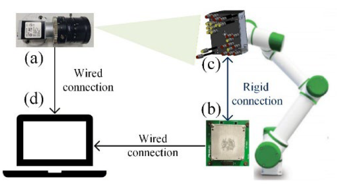
Figure 2.
System flowchart.
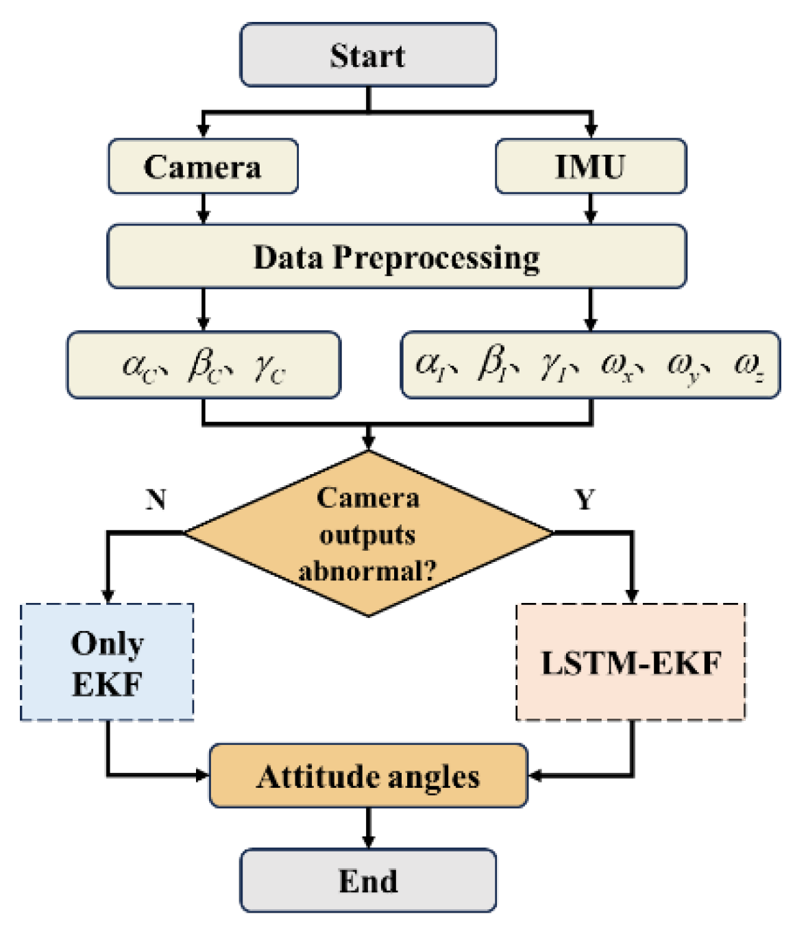
Figure 3.
LSTM structure.
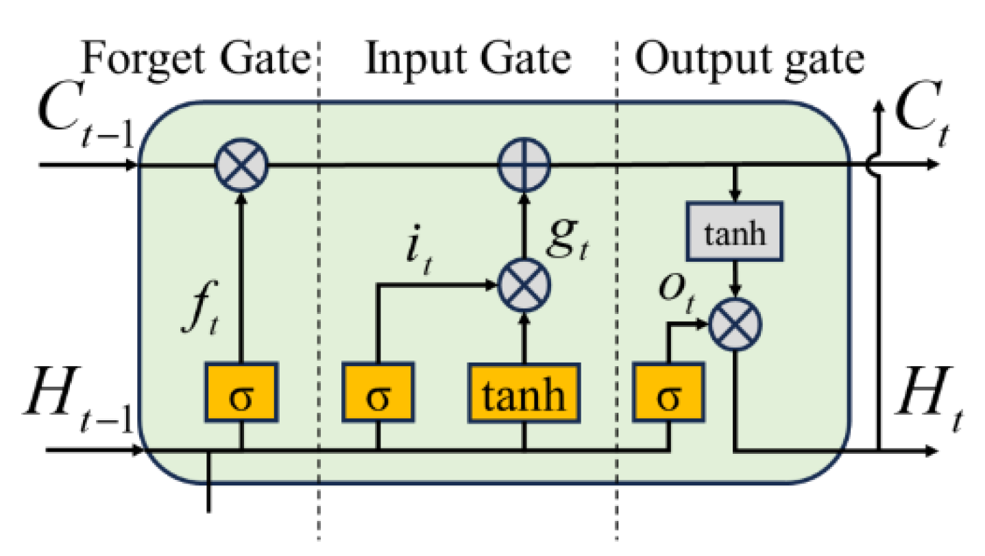
Figure 4.
LSTM-EKF fusion algorithm framework.
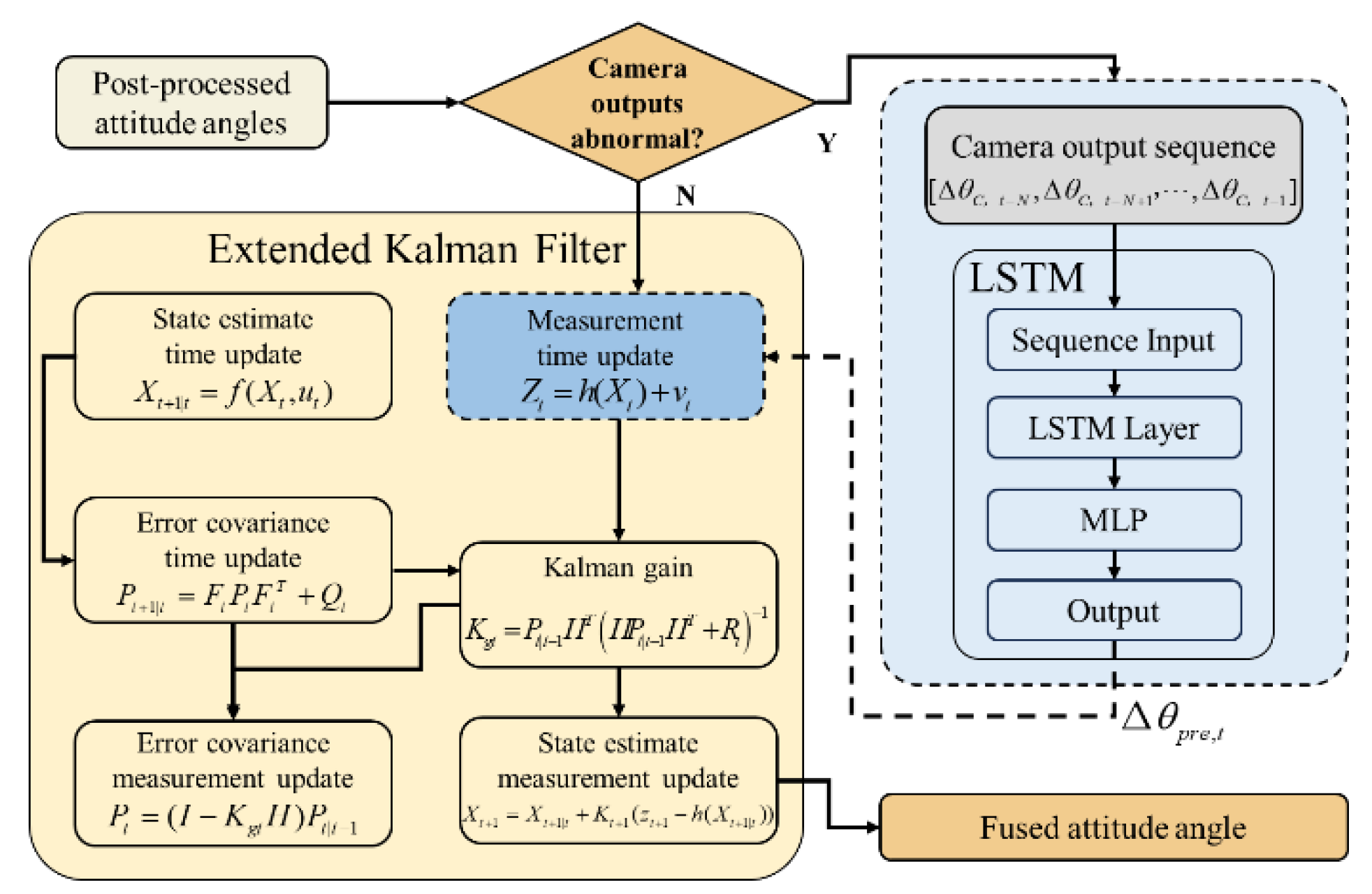
Figure 5.
The result of Input sequence length time-series cross-validation.
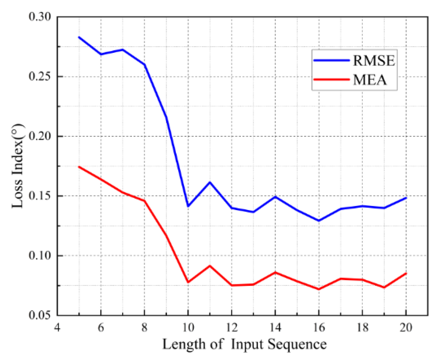
Figure 6.
The effect of different network parameters on the results.
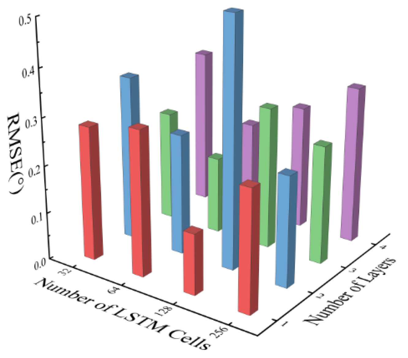
Figure 7.
The LSTM network structures.
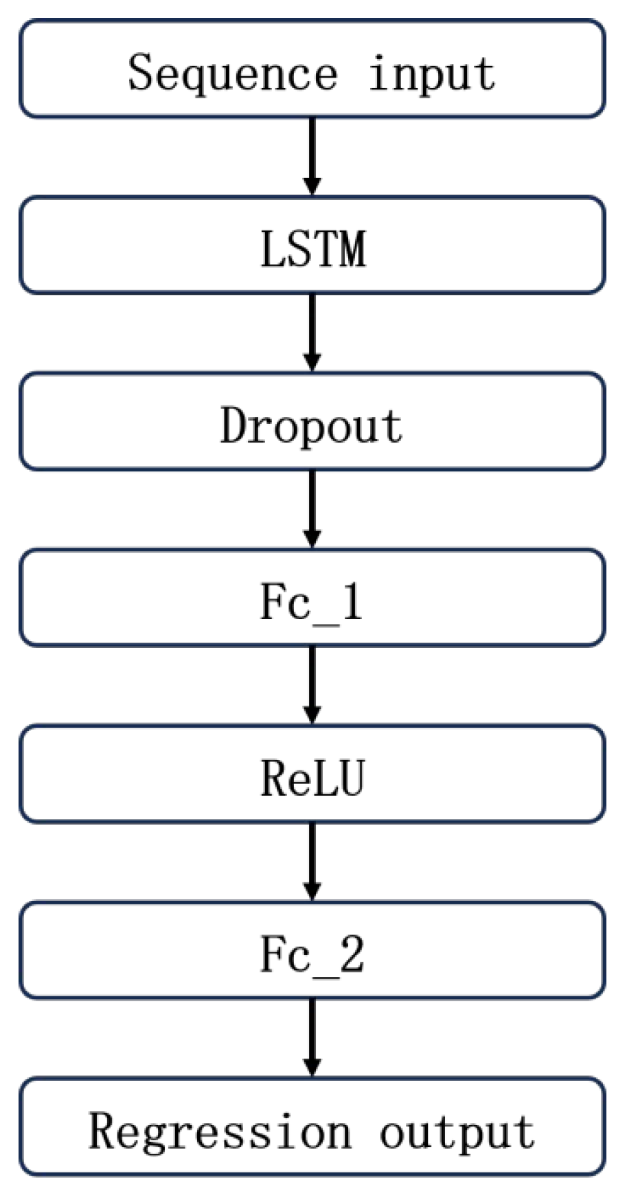
Figure 8.
Error of simulation results.
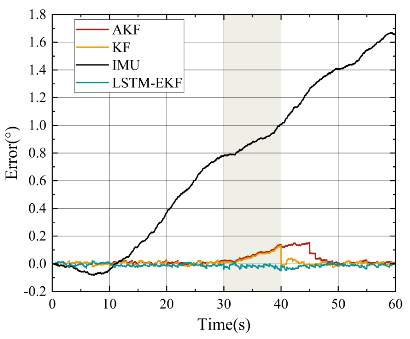
Figure 9.
Experimental platform.
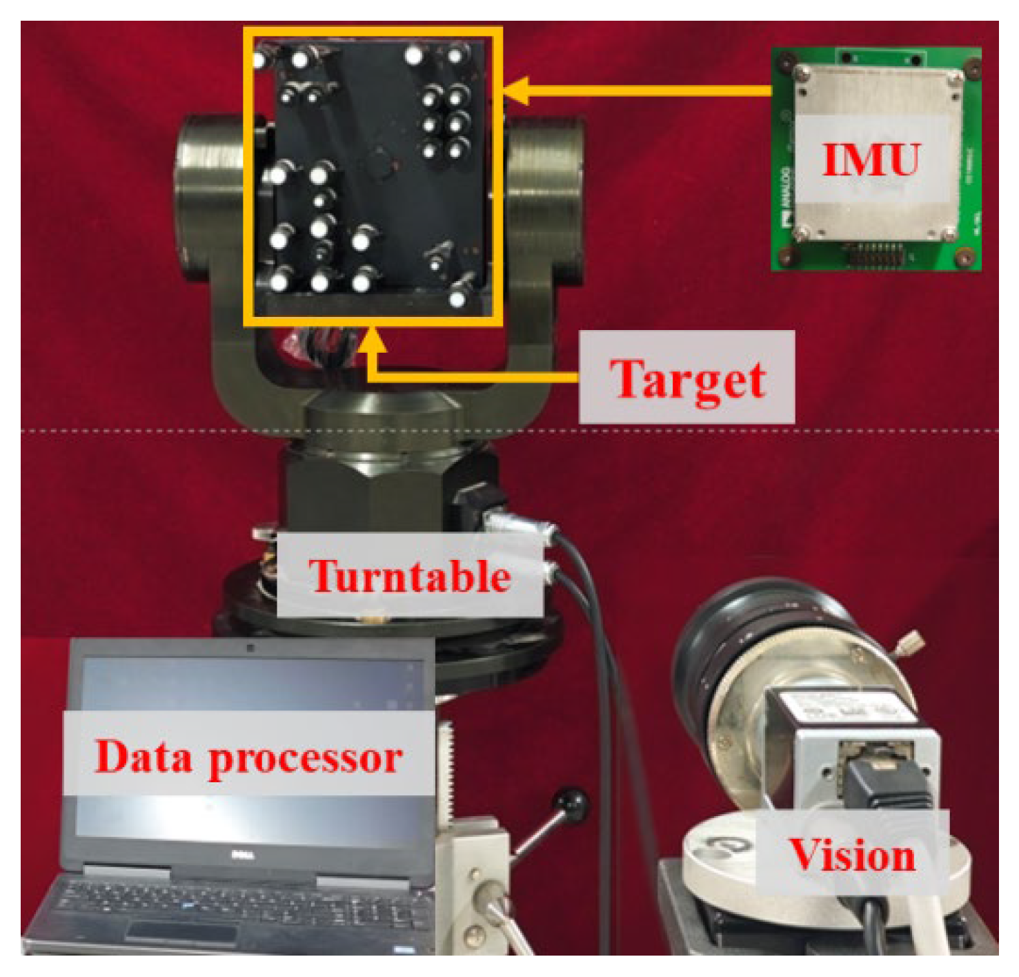
Figure 10.
Rotation measurement results under long-term reciprocating motion.
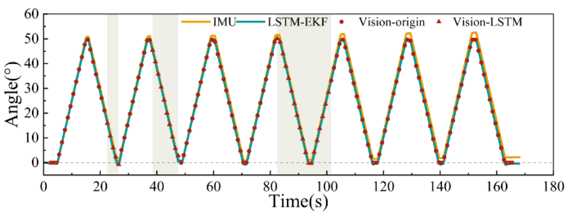
Figure 11.
Error comparison among fusion methods. (a) 5-frame visual loss. (b) 10-frame visual loss. (c) 20-frame visual loss.
Figure 11.
Error comparison among fusion methods. (a) 5-frame visual loss. (b) 10-frame visual loss. (c) 20-frame visual loss.
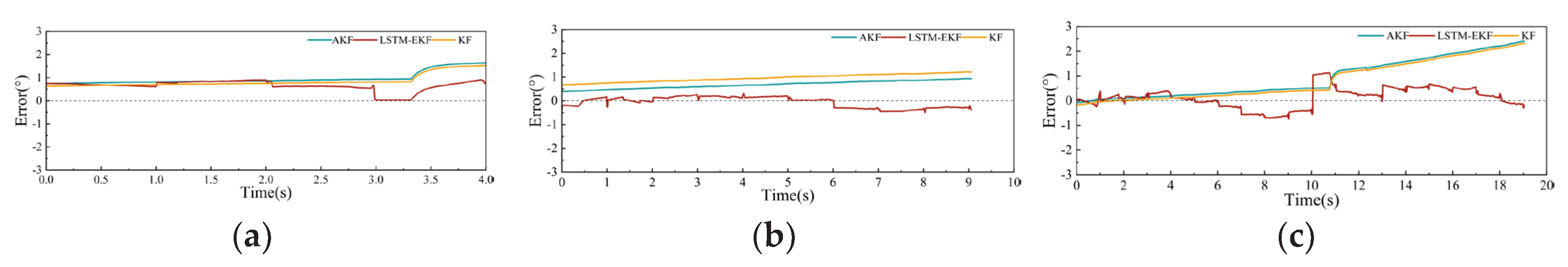
Figure 12.
Fusion results with changes in the number of missing frames from the camera.
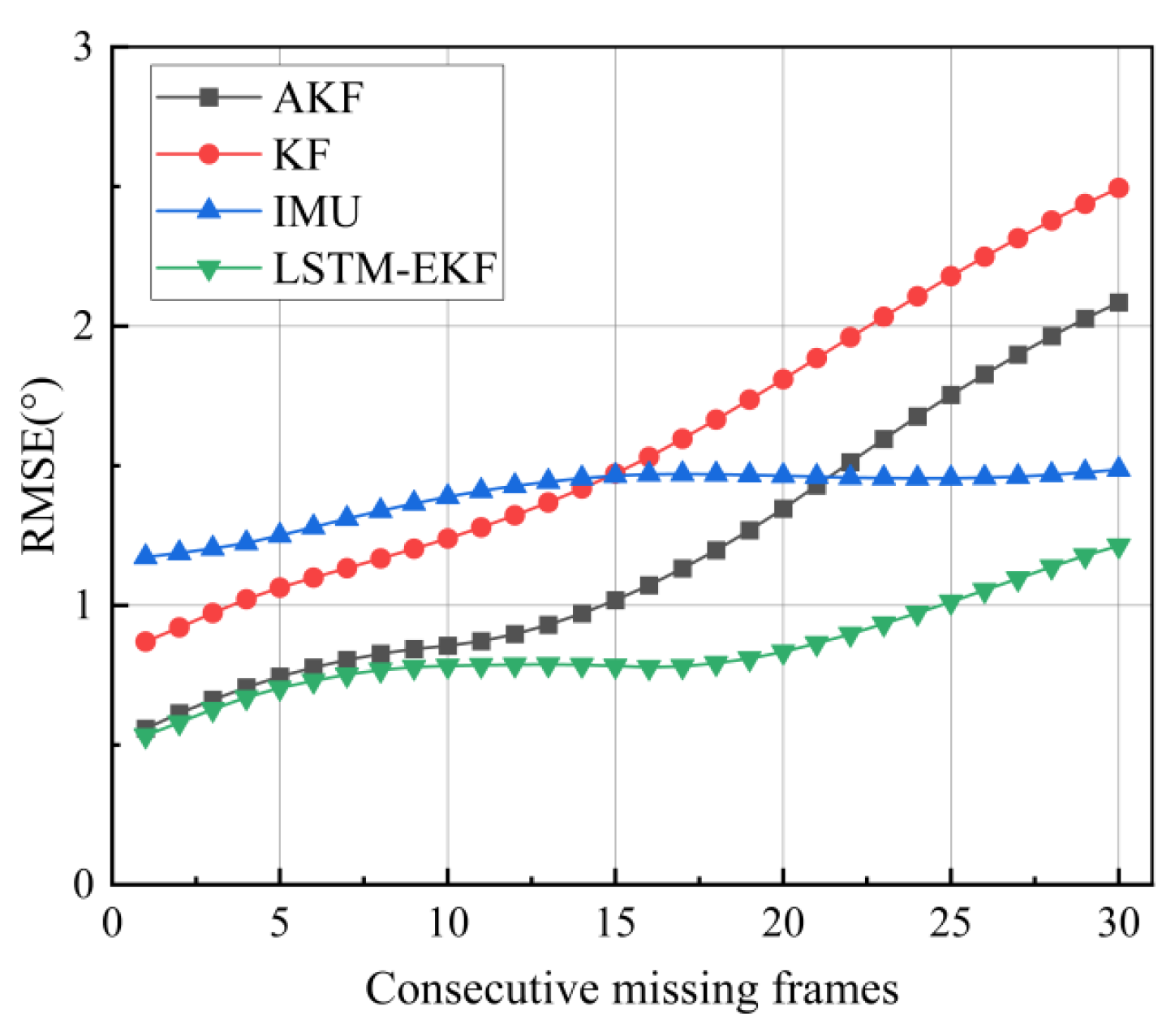
Figure 13.
Measurement results with 80° rotation.
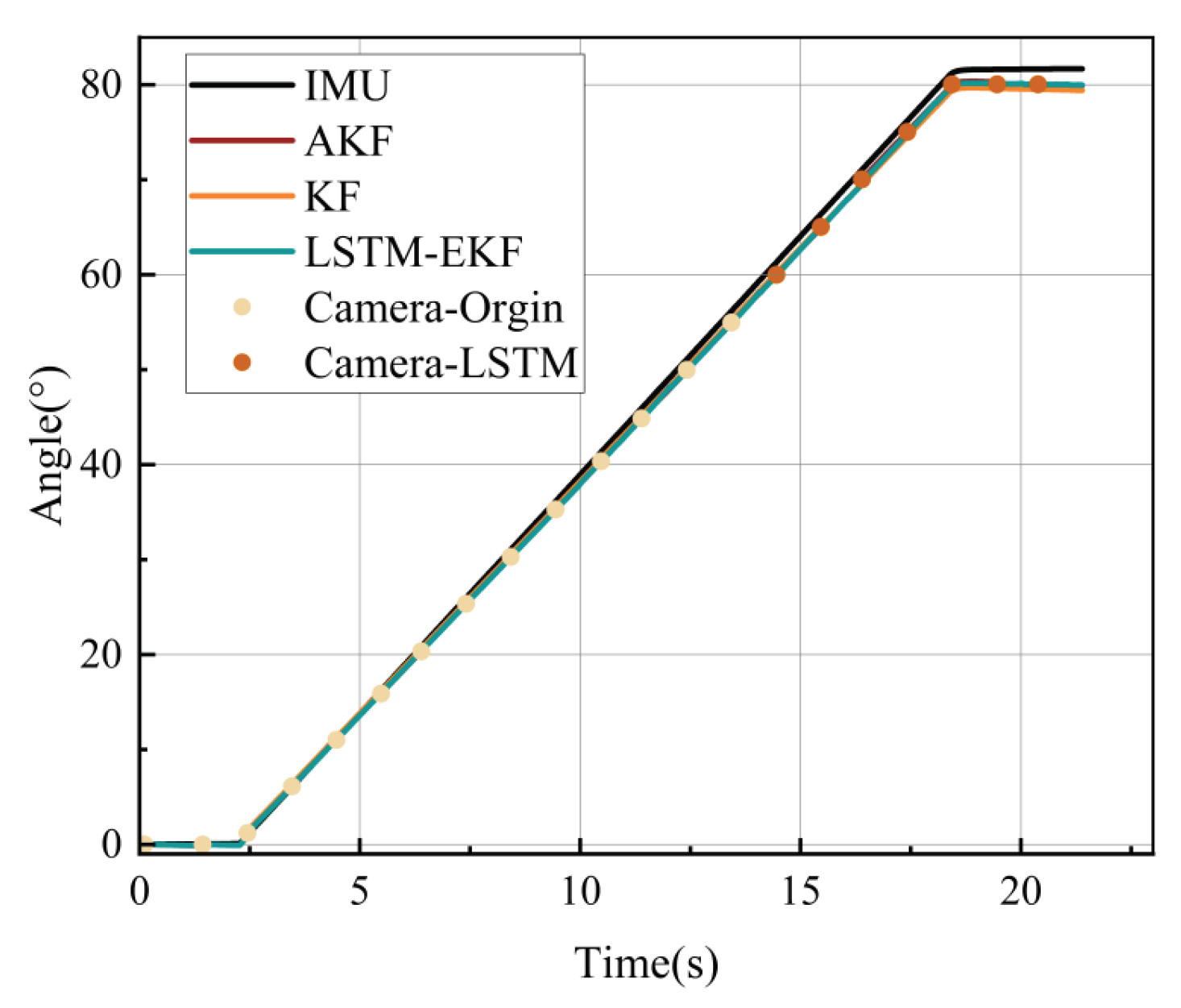

Table 1.
Simulation conditions.
| Sensor | Parameters | Value |
|---|---|---|
| IMU | Gyroscope bias | 0.01°/h |
| Angular velocity random walk | ||
| Sampling interval | 0.01s | |
| Camera | Measurement bias | 0.01° |
| Sampling interval | 1s |
Table 2.
LSTM parameters.
| Parameters | Value |
|---|---|
| Input dimensions | 3×16 |
| Number of LSTM layers | 1 |
| Number of LSTM layer cells | 64 |
| Dataset size | 2400 |
| Initial learning rate | 0.001 |
| Learning rate decay interval | 100 |
| Learning rate decay factor | 0.1 |
| L2 regularization coefficient | 0.01 |
Table 3.
Performance Comparison of Fusion Algorithms.
| Parameters | KF/° | AKF/° | LSTM-EKF/° | |
|---|---|---|---|---|
| Whole | MAE | 0.490 | 0.535 | 0.396 |
| RMSE | 0.668 | 0.698 | 0.469 | |
| ME | 0.418 | 0.518 | 0.294 | |
| Vision Loss | MAE | 0.864 | 0.848 | 0.344 |
| RMSE | 1.054 | 1.049 | 0.428 | |
| ME | 0.856 | 0.845 | 0.121 | |
Table 4.
Absolute error of different methods.
| Reference angle | IMU/° | LSTM-EKF/° | AKF/° | |
|---|---|---|---|---|
| Within visual range | 0 | 0.122 | 0.051 | 0.077 |
| 5 | 0.173 | 0.091 | 0.106 | |
| 10 | 0.213 | 0.104 | 0.152 | |
| 15 | 0.226 | 0.117 | 0.186 | |
| 20 | 0.276 | 0.128 | 0.191 | |
| 25 | 0.290 | 0.136 | 0.221 | |
| 30 | 0.374 | 0.157 | 0.233 | |
| 35 | 0.407 | 0.160 | 0.248 | |
| 40 | 0.526 | 0.157 | 0.225 | |
| 45 | 0.628 | 0.150 | 0.220 | |
| 50 | 0.720 | 0.151 | 0.284 | |
| 55 | 0.779 | 0.182 | 0.267 | |
| Out of visual range | 60 | 0.812 | 0.204 | 0.342 |
| 65 | 0.848 | 0.221 | 0.352 | |
| 70 | 0.858 | 0.236 | 0.379 | |
| 75 | 0.883 | 0.255 | 0.334 | |
| 80 | 1.001 | 0.264 | 0.384 | |
Table 5.
Ablation experiment.
| Algorithm | Experiment 1/° | Experiment 2/° | Experiment 3/° |
|---|---|---|---|
| LSTM-EKF | 0.463 | 0.753 | 0.14 |
| Only EKF | 0.972 | 0.964 | 0.258 |
Disclaimer/Publisher’s Note: The statements, opinions and data contained in all publications are solely those of the individual author(s) and contributor(s) and not of MDPI and/or the editor(s). MDPI and/or the editor(s) disclaim responsibility for any injury to people or property resulting from any ideas, methods, instructions or products referred to in the content. |
© 2026 by the authors. Licensee MDPI, Basel, Switzerland. This article is an open access article distributed under the terms and conditions of the Creative Commons Attribution (CC BY) license.
Copyright: This open access article is published under a Creative Commons CC BY 4.0 license, which permit the free download, distribution, and reuse, provided that the author and preprint are cited in any reuse.


