
Submitted:
11 January 2026
Posted:
12 January 2026
You are already at the latest version
Abstract
The standard $\varepsilon$--$\delta$ definition of continuity is inherently quantitative, yet the precise dependence of the admissible radius $\delta$ on the accuracy $\varepsilon$ and the base point $x_0$ is rarely treated as an independent mathematical object. In this paper, we introduce the \textit{radius of continuity} through two variants: the radius of pointwise continuity and the radius of uniform continuity, defined as explicit numerical invariants that capture the maximal symmetric neighborhood on which a real-valued function maintains a prescribed tolerance. We establish the fundamental structural properties of these radii, including their behavior under algebraic operations such as sums, products, and compositions, and demonstrate their inverse relationship to the classical modulus of continuity. Furthermore, we prove that the finiteness pattern of these radii characterizes constant versus non-constant functions. To illustrate the utility of this framework, we derive closed-form expressions for the pointwise radius of quadratic polynomials and the uniform radius of the normal probability density function. These examples highlight how the radius of continuity encodes geometric and probabilistic features, such as local curvature and global scale parameters. Ultimately, this perspective bridges the gap between real analysis and quantitative methods in metric geometry, offering a concrete measure of the stability of a function's continuity.
Keywords:
continuity
; foundations
; elementary functions
MSC: 26A03; 26A06; 26A09; 26A15
“When you can measure what you are speaking about, and express it in numbers, you know something about it.”
— Lord Kelvin (1824–1907)
1. Introduction
1.1. Real-Valued Functions and Continuity
We work throughout in the function space of all real-valued functions defined on the real line. Within this space, continuity remains one of the central regularity properties. In standard real analysis, a function is said to be continuous at a point if for every there exists a such that for all
This – definition, and its various equivalent formulations in terms of sequences or inverse images of open sets, provides the standard language for studying local behaviour of real-valued functions [1,2].
A stronger notion, uniform continuity on a set , requires that for each there is a single that statement (1) works simultaneously for all points . Uniform continuity is closely related to the classical modulus of continuity of a function, which quantifies the size of oscillations at a given spatial scale and plays an important role in analysis on metric spaces and in regularity theory [3].
In the present paper we remain in this classical setting—real-valued functions on equipped with the Euclidean metric —but shift the emphasis from the qualitative statement “f is (uniformly) continuous” to a quantitative description of how far one can move in the domain while preserving a prescribed -accuracy in the range. Our goal is to refine the usual continuity framework by associating to each function a family of radii that encode the local and global “size” of its continuity.
1.2. Motivation
The – definition of continuity is inherently quantitative: given and a point , any admissible determines a neighbourhood on which f fluctuates by at most . However, in most textbooks and classroom proofs one only exhibits some convenient ; the collection of all admissible radii is rarely examined systematically [1,2]. This leaves several natural quantitative questions unanswered. For instance: for a fixed accuracy level , what is the largest radius around on which the -tolerance still holds? How does this maximal radius depend on and on the structure of f?
In earlier work, the author proposed a global classification of the function space into blocks according to the cardinalities of the sets of continuity and differentiability points [4]. That framework was at macroscale and qualitative: it distinguished functions by the size and location of their continuity sets but did not deal with it in microscale nor quantify the strength of continuity at individual points or uniformly on . The present paper aims to complement that perspective by introducing and studying the radius of continuity at a point and its uniform counterpart.
More precisely, for a given function f, point , and accuracy level , we consider the set of all radii for which the – condition holds, and define the pointwise radius of continuity as the supremum of this set. Analogously, we define the uniform radius of continuity by taking the largest radius that works simultaneously for all . These radii can be expressed in terms of pointwise and uniform oscillation functions, thereby connecting our viewpoint to classical moduli of continuity [3,5,6,7].
This radius-based approach has several advantages. It packages the infinitary quantifiers in the usual continuity definition into concrete numerical invariants; it allows for explicit closed-form computations in important families of functions (for example, quadratic polynomials or normal density functions); and it offers a way to compare the “stability” of different functions under perturbations of the input. At a more conceptual level, radii of continuity provide a bridge between textbook – arguments and quantitative notions that are commonly used in modern analysis and numerical applications, where explicit control over neighbourhood sizes is often required.
1.3. Organization of the Paper
The remainder of the paper is organized as follows. In Section 2 we introduce the pointwise and uniform radii of continuity, develop equivalent descriptions in terms of local and uniform oscillation, and establish basic structural properties. In particular, we characterize non-constant and constant functions in through the finiteness or infiniteness of their associated radii. Section 3 is devoted to explicit computations: we derive a closed-form formula for the pointwise radius of continuity of a quadratic polynomial and analyze the uniform radius of continuity for the normal probability density function, illustrating how the abstract theory translates into concrete expressions. Finally, Section 4 concludes the paper with a discussion on the main findings and outlines several directions for future work.
2. The Radius of Continuity: Definitions & General Properties
2.1. Radius of Pointwise Continuity
In this section, we introduce, for each function f, point , and accuracy level , the set of all radii for which the usual – condition holds at , and we define the pointwise radius of continuity as the supremum of this set (Figure 1). This quantity admits an equivalent description in terms of the local oscillation of f [5,6] on the symmetric interval , or, after a shift of variables, in terms of an h-dependent oscillation around the origin. We then collect a number of elementary but useful properties of , including an evenness property in the spatial variable, natural scaling relations, and inequalities that arise when f is globally Lipschitz. Further bounds describe how radii behave under algebraic operations: the radius for a sum or product of functions can be estimated in terms of the radii of the individual factors, and similar control holds for compositions under mild regularity conditions. These results show that the radius of continuity is compatible with the standard algebraic operations in , and can therefore be propagated through many common constructions. Finally, we prove that the finiteness pattern of characterizes whether f is constant or not: a non-constant function necessarily has finite radius at some continuity point, whereas a function with infinite radius everywhere must be constant.
Definition 1
(Radius of Pointwise Continuity). Let be a real-valued function with a nonempty set of continuity points . For and define the pointwise admissible continuity admissible radius as:
Remark 1
(Shifted-h formulation of and ). Equivalently, in terms of the local oscillation
we have:
Proposition 1
(Properties of Radius of Pointwise Continuity). Let . Then, for and the radious of pointwise continuity has the following properties:
- (A)
- Single–function properties.
- (i)
- Evenness. If f is even, then .
- (ii)
- Scaling. If , then ; if , then .
- (iii)
- Large– for bounded f. If everywhere and , then for all (the constant is sharp in general).
- (iv)
- Monotonicity in . If , then .
- (v)
- Input translation. For one has .
- (vi)
- Lipschitz lower bound. If f is L-Lipschitz on [8], then ; in particular, if f is globally L-Lipschitz, .
- (vii)
- Continuity criterion. f is continuous at iff for every .
- (B)
- Two–function properties.
- (viii)
- Composition. If g is continuous at with modulus η (i.e., ), then
- (ix)
-
Sum (lower bound). For and any ,(There is no universal matching upper bound; e.g., , .)
- (x)
-
Linear combination (lower bound). For and any ,with the convention from (ii) when a coefficient is 0.
- (xi)
- Product (one convenient bound). If on , then for any ,
Proof.
(i) for even f (substitute ). (ii) ; for , . (iii) . (iv) . (v) . (vi) On , ; take . (vii) Equivalent to the ε–δ definition. (viii) If then ; hence . (ix) By triangle inequality and a split ; the counterexample , shows no universal upper bound. (x) Combine (ii) with (ix). (xi) Use , bound on , and choose the two tolerances to sum to ε. □
Theorem 1
(Characterization of Radius of Pointwise Continuity). Let be a real-valued function with a nonempty set of continuity points . For and the following are equivalent:
- (i)
- f is non-constant.
- (ii)
- There is there exists such that .
Proof.
(ii) ⇒ (i). Suppose (ii) holds and, towards a contradiction, assume f is constant: . Fix any (indeed, ) and any . Then for all x, so and thus , contradicting (ii).
(i) ⇒ (ii). Assume f is non-constant. Fix . Then there are with and . Set
Since , at least one of a or b (call it p) satisfies . Consequently, any forces the open interval to contain p, and hence to contain a point where . By the definition of we obtain the finite bound
This supplies, for the given , an explicit with . Since was arbitrary, (ii) follows. □
Corollary 1.
With defined as above, the following are equivalent:
- (i)
- f is constant.
- (ii)
- For every and every , we have .
2.2. Radius of Uniform Continuity
In this section we pass from the local picture at a single point to a global one by introducing, for each function f and accuracy level , the set of all radii that make the – condition hold simultaneously for every . The uniform radius of continuity is then defined as the supremum of this set and measures, in a single number, how far one can move anywhere in the domain without exceeding the prescribed error (Figure 2). We show that admits a clean formulation in terms of the uniform oscillation of f [5,7], obtained by taking the supremum of over all pairs of points at distance less than . This viewpoint allows us to derive a collection of general properties of and to compare it directly with the pointwise radius , for instance by bounding the former in terms of the infimum of the latter over all base points. In particular, whenever f is uniformly continuous, the uniform radius is strictly positive for each , while for merely pointwise continuous functions may degenerate to zero even though each remains positive. Finally, we obtain a characterization analogous to the pointwise case: the pattern of finiteness or infiniteness of completely determines whether f is constant or non-constant, so that the uniform radius encodes global regularity information in a quantitative form.
Definition 2
(Radius of Uniform Continuity). Let be a real-valued function with a nonempty set of continuity points . For define the uniform admissible radius as:
Remark 2
(Shifted-h formulation of and ). For the uniform case, introduce the uniform local oscillation
Then:
Proposition 2
(Properties of Radius of Uniform Continuity). Let . Then, for the radius of uniform continuity has the following properties:
- (A)
- Single–function properties.
- (i)
- Scaling. If , then ; if , then .
- (ii)
- Monotonicity in . If , then .
- (iii)
- Translation/reflection invariance. For or , we have .
- (iv)
- Large– for bounded f. If everywhere and , then (sharp in general).
- (v)
- Lipschitz lower bound. If f is globally L-Lipschitz, then .
- (vi)
- Uniform continuity criterion. f is uniformly continuous on iff for every .
- (vii)
- Link to pointwise radii. .
- (B)
- Two–function properties.
- (viii)
- Composition. If g admits a global modulus η with , then
- (ix)
-
Sum (lower bound). For any ,(There is no universal matching upper bound; e.g., , .)
- (x)
-
Linear combination (lower bound). For and any ,with the convention in (i) if a coefficient is 0.
- (xi)
- Product (global bounds). If and on , then for any ,
Proof.
(i). If , . (ii) Inclusion of level sets . (iii) Both translations and leave unchanged: and . (iv) For all , . (v) Global Lipschitz gives ; take . (vi) This is exactly the ε–δ definition of uniform continuity. (vii) If then, fixing any , , hence ; take sups and then the infimum over . (viii) If then ; thus . (ix) Triangle inequality with split . (x) Apply (i) to and and then (ix). (xi) Using , pick and and invoke the uniform radii of and , respectively. □
Theorem 2
(Characterization of Radius of Uniform Continuity ). Let be a real-valued function with a nonempty set of continuity points . For the following are equivalent:
- (i)
- f is non-constant ⟺
- (ii)
- There exists , .
Proof.
If f is constant, then for all , so and .
Conversely, suppose f is non-constant, pick with and set . Then for any , the pair satisfies but , so . Hence
This mirrors the pointwise result with and shows the same finite-radius phenomenon in the uniform setting. □
Corollary 2.
With defined as above, the following are equivalent:
- (i)
- f is constant.
- (ii)
- For every , we have .
3. Examples and Explicit Computations
In this section we illustrate the general theory by working out two concrete families of functions in detail. First, in Section 3.1 we study the quadratic polynomial and compute an explicit closed-form expression for the pointwise radius of continuity in terms of , , and the coefficients . This formula allows us to analyze how the radius behaves as the base point moves along the real line, showing in particular that it decays at infinity and attains its maximal value at the vertex . We also identify a simple symmetry condition on the coefficients under which the radius becomes an even function of . Second, in Section 3.2 we turn to a probabilistic example and consider the normal density with parameters and . Using an explicit Lipschitz constant for this density, we derive a closed-form expression for the uniform radius of continuity , which exhibits a piecewise behaviour in : linear growth up to a threshold followed by saturation at infinity. The resulting formula makes transparent how the uniform radius depends on the scale parameter , and thereby demonstrates how our radius-of-continuity framework captures both geometric and probabilistic features of a function in a quantitative way.
3.1. Radius of Pointwise Continuity of the Quadratic Polynomial
Example 1.
Let be the quadratic polynomial. We calculate in the following three steps:
Step 1 — Increment at .
Step 2 — Exact oscillation on .
Step 3 — Solve .
Behavior and Evaluations
We have:
- 1.
- Asymptotic Equivalency:
- 2.
- Left/Right Branch:
- 3.
- Vertex:
- 4.
- Symmetry Condition:
- 5.
- Figure 3 presents the radius of pointwise continuity for the quadratic polynomial function.
3.2. Radius of Uniform Continuity of the General Normal Probability Density Function
Example 2.
Let be the probability density of the normal distribution . We calculate as follows:
Step 1 (Function and derivative).
Step 2 (Global Lipschitz constant). Let . Set . For , has
and g is maximized at with . Hence
Step 3 (Uniform oscillation upper bound). By the mean value theorem, for all and ,
Taking the sup over x and gives
Step 4 (Sharpness—matching lower bound). Choosing x near (where is maximal) and with the sign of ,
so for any and small enough δ,
Together with (23),
Step 5 (Saturation ceiling). . Thus
We have:
- 1.
- Asymptotic (small ε):
- 2.
-
Parameter dependence:The radius is independent of μ. For fixed , grows quadratically in σ (). The threshold decreases like , and the break radius increases linearly in σ.
- 3.
-
Monotonicity and jump:is strictly increasing and linear on with slope . It has a jump at :
- 4.
-
Scaling identity:If is the pdf for distribution and is pdf for the standard normal distribution, then for :
- 5.
- Figure 4 presents the radius of uniform continuity for the normal probability density function.
4. Discussion
4.1. Summary of the Radius-of-Continuity Viewpoint
In this paper we proposed the radius of continuity as a quantitative refinement of the classical – definition for real-valued functions on . For each function f, point , and accuracy level , the pointwise radius captures the largest symmetric neighbourhood on which the deviation remains below . On the global side, the uniform radius measures how far we may move anywhere in the domain while enforcing the same tolerance uniformly in . We showed that both radii admit natural descriptions in terms of pointwise and uniform oscillation, which clarify their structural properties and their behaviour under algebraic operations such as sums, products, and compositions. The resulting invariants distinguish constant functions from non-constant ones and allow us to compare the “stability” of different functions on a common quantitative scale. The explicit computations for a quadratic polynomial and for the normal density illustrate how these abstract notions lead to concrete formulas that encode geometric and probabilistic information about the underlying functions.
4.2. Relation to Classical Moduli of Continuity and Proofs
From a conceptual perspective, the radii and can be viewed as inverse objects to the pointwise and uniform moduli of continuity. While a modulus assigns, for each spatial scale , an upper bound on , our radii fix a vertical tolerance and ask for the largest admissible horizontal scale. Thus the radius-of-continuity framework repackages the traditional – quantifiers into numerical invariants that are often easier to visualize and to compute explicitly. At the same time, the proofs in Section 2 make clear that the standard techniques used in real analysis – arguments—such as bounding slopes, factoring expressions, or exploiting Lipschitz estimates—extend seamlessly to the analysis of radii. In this sense the present approach does not replace the classical theory, but rather sits on top of it: the same inequalities that certify continuity now yield quantitative control of and , providing a bridge between elementary real analysis and more metric-oriented notions of regularity [9,10].
4.3. Future Work
Several directions for further investigation emerge naturally from this study. First, it would be interesting to develop a more systematic comparison between the pointwise and uniform radii, for example by identifying classes of functions for which can be reconstructed from the family . Second, in the special case of absolutely continuous functions, one may hope to express radii in terms of the derivative, leading to integral or differential characterizations that parallel the usual connections between absolute continuity and bounded variation [11]. Third, the definitions extend verbatim to general metric spaces, and it remains to explore how the underlying geometry (for instance, doubling properties or curvature bounds) constrains the possible profiles of and . Finally, higher dimensional examples—such as multivariate polynomials, radial functions, or densities on —could provide additional insight into how radii interact with phenomena like anisotropy and directional derivatives, and how they might be used in applications that require explicit control over perturbations in several variables.
Funding
This research received no external funding.
Acknowledgments
Special thanks go to my wife, Bahareh, as many of the concepts developed here took shape during our casual conversations while hiking in nature.
Conflicts of Interest
The author declares no conflicts of interest.
References
- Abbott, S. (2015). Understanding Analysis (2nd ed.). Springer. [CrossRef]
- Tao, T. (2016). Analysis I (3rd ed.). Springer. [CrossRef]
- Heinonen, J. (2001). Lectures on Analysis on Metric Spaces. Springer. [CrossRef]
- Soltanifar, M. (2023). A Classification of Elements of Function Space F(R,R). Mathematics, 11(17), 3715. [CrossRef]
- Davidson, K. R., & Donsig, A. P. (2010). Real Analysis and Applications: Theory in Practice. Springer. [CrossRef]
- Pugh, C. C. (2015). Real Mathematical Analysis (2nd ed.). Springer. [CrossRef]
- Aksoy, A. G., & Khamsi, M. A. (2010). A Problem Book in Real Analysis. Springer. [CrossRef]
- Cobzaş, Ş., Miculescu, R., & Nicolae, A. (2019). Lipschitz Functions. Springer. [CrossRef]
- Kohlenbach, U., López-Acedo, G., & Nicolae, A. (2019). Moduli of Regularity and Rates of Convergence for Fejér Monotone Sequences. Israel Journal of Mathematics, 232, 261–297. [CrossRef]
- Kohlenbach, U. (2024). On the Computational Content of Moduli of Regularity and Their Logical Strength. Manuscript. https://www2.mathematik.tu-darmstadt.de/~kohlenbach/.
- Axler, S. (2020). Measure, Integration & Real Analysis. Springer. [CrossRef]
Figure 1.
Geometric illustration of the pointwise radius of continuity for a continuous function f at a fixed point : the horizontal band in the range is matched with symmetric intervals in the domain. Admissible radii correspond to intervals on which , while the maximal radius is attained at the first intersection of the graph of f with the -boundary.
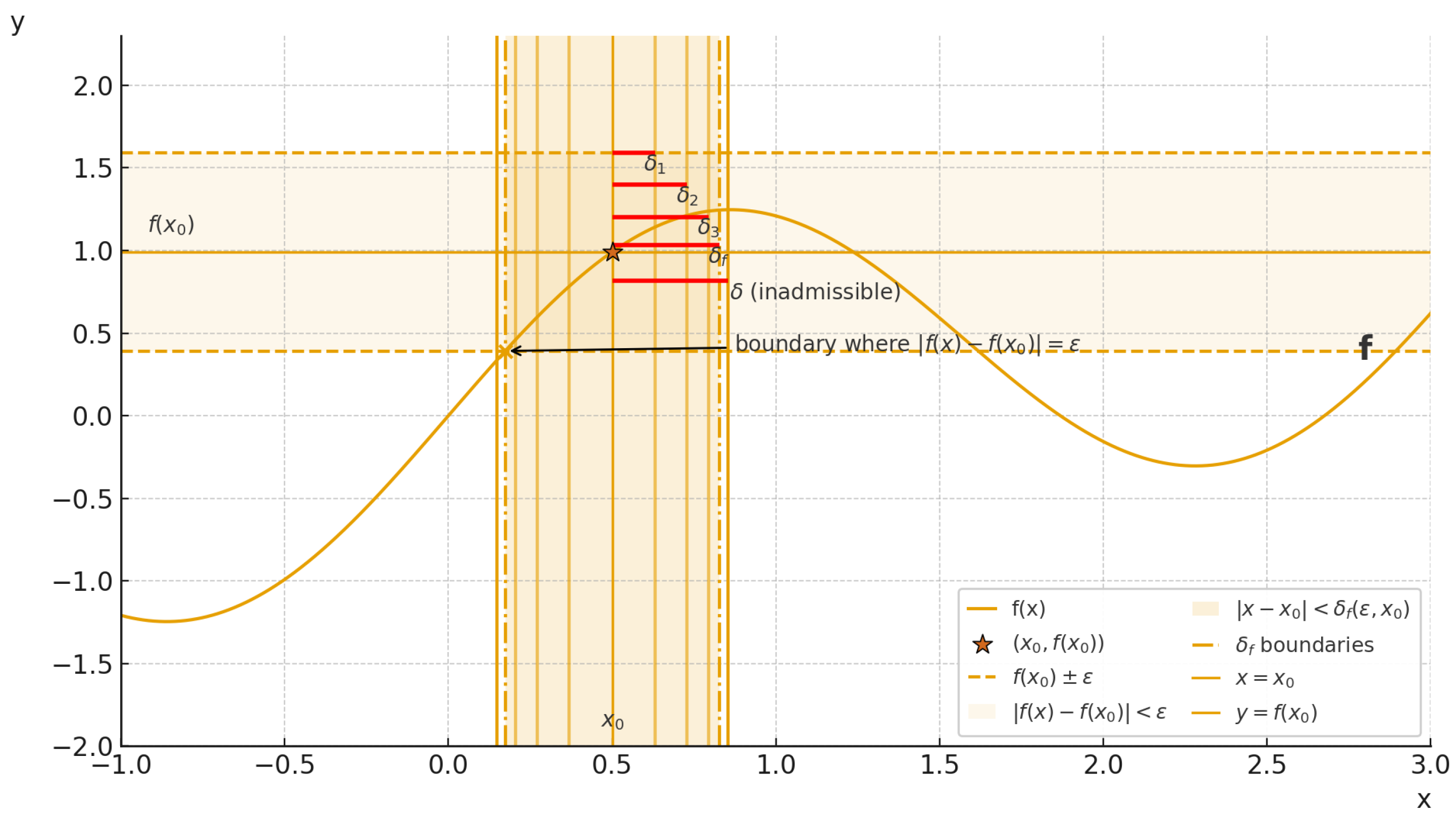
Figure 2.
Geometric illustration of the uniform radius of continuity : a single radius controls all pairs of points with , forcing their function values to lie in the same horizontal -band around . The highlighted pair and shows that, whenever , the vertical lines through and remain inside this band, illustrating that is chosen independently of the base point.
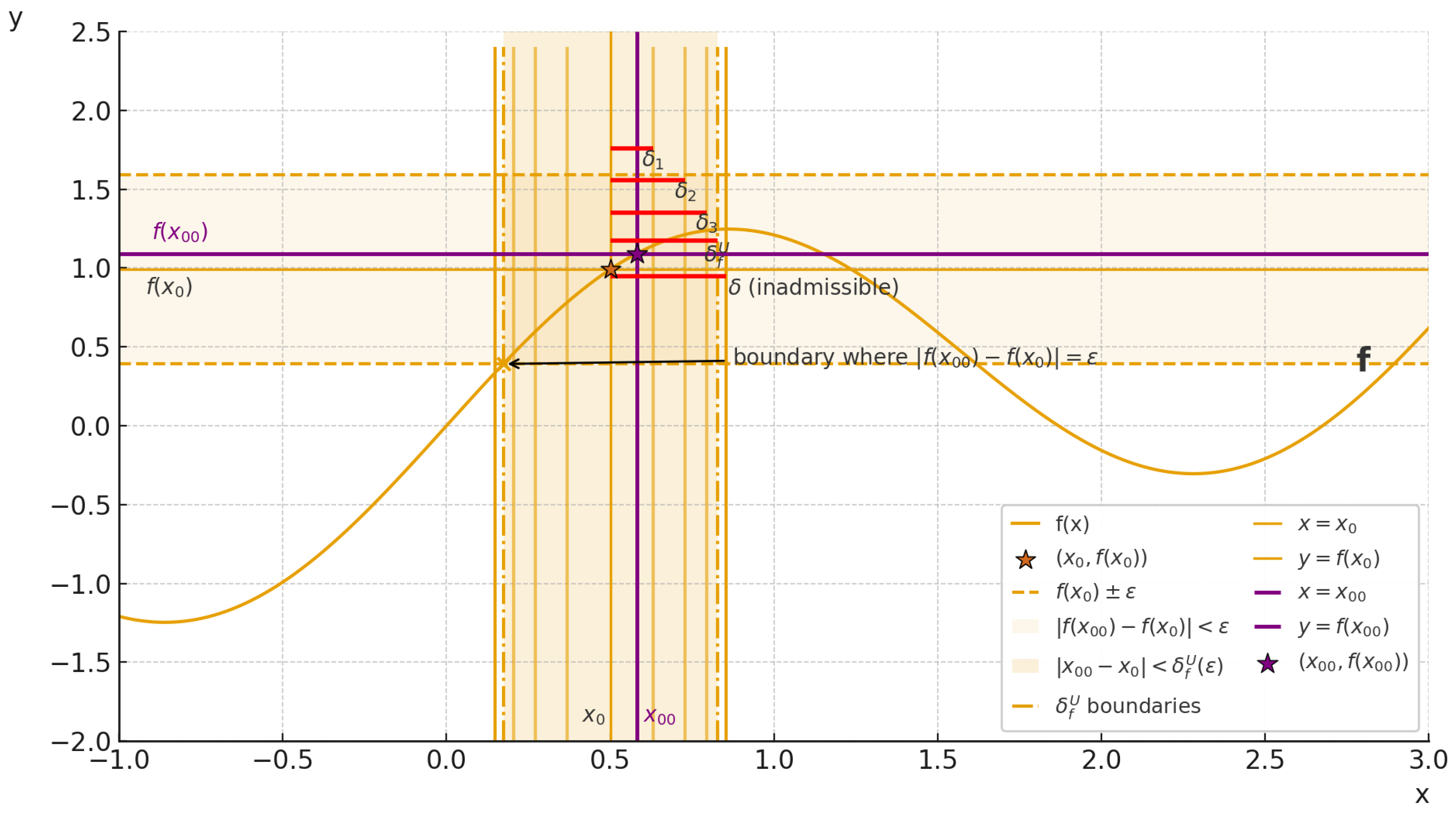
Figure 3.
Pointwise radius of continuity for the quadratic on with . The anti-symmetric curve attains its maximum at the vertex and decays rapidly as , illustrating how the admissible neighbourhood size shrinks away from the point of minimal slope.
Figure 3.
Pointwise radius of continuity for the quadratic on with . The anti-symmetric curve attains its maximum at the vertex and decays rapidly as , illustrating how the admissible neighbourhood size shrinks away from the point of minimal slope.
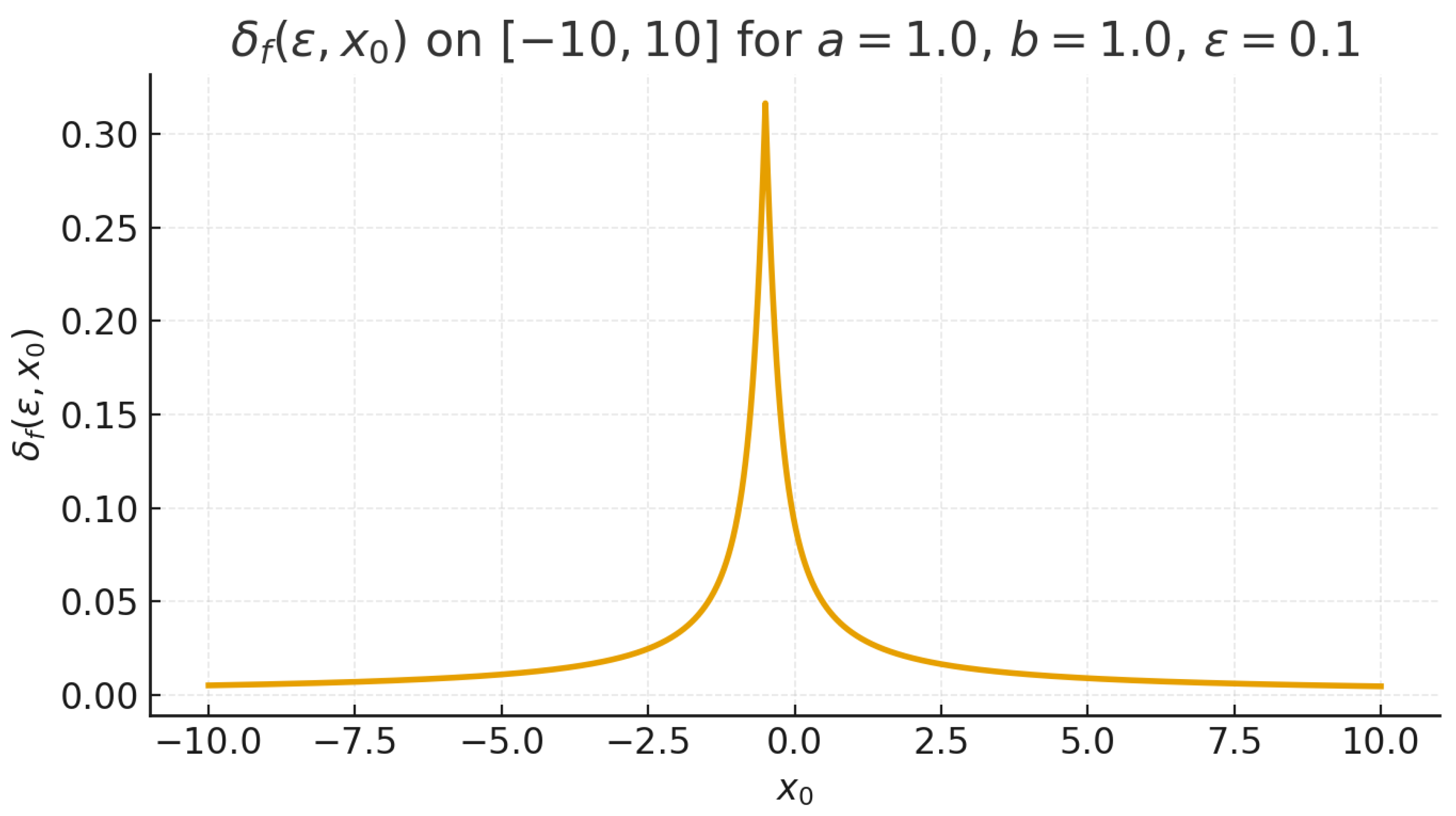
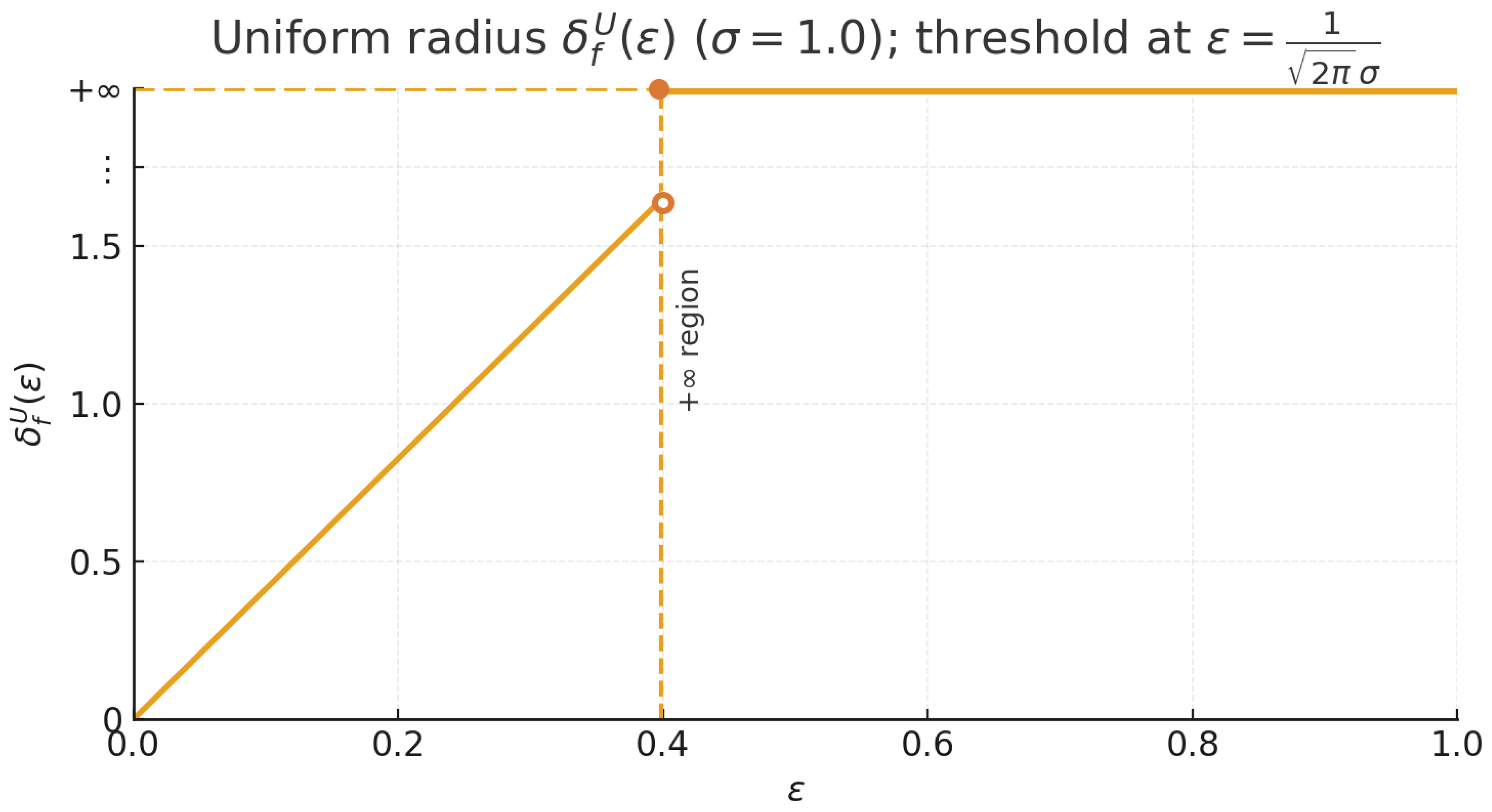
Figure 4.
Uniform radius of continuity for the Gaussian density with . For small the radius grows linearly until the critical value ; beyond this threshold the -band already covers the full range of f and becomes infinite.
Figure 4.
Uniform radius of continuity for the Gaussian density with . For small the radius grows linearly until the critical value ; beyond this threshold the -band already covers the full range of f and becomes infinite.
Disclaimer/Publisher’s Note: The statements, opinions and data contained in all publications are solely those of the individual author(s) and contributor(s) and not of MDPI and/or the editor(s). MDPI and/or the editor(s) disclaim responsibility for any injury to people or property resulting from any ideas, methods, instructions or products referred to in the content. |
© 2026 by the authors. Licensee MDPI, Basel, Switzerland. This article is an open access article distributed under the terms and conditions of the Creative Commons Attribution (CC BY) license (http://creativecommons.org/licenses/by/4.0/).
Copyright: This open access article is published under a Creative Commons CC BY 4.0 license, which permit the free download, distribution, and reuse, provided that the author and preprint are cited in any reuse.


