
Submitted:
08 January 2026
Posted:
09 January 2026
You are already at the latest version
Abstract
Finite element analysis (FEA) remains the gold standard for simulating piezoelectric microactuators because it resolves coupled electromechanical fields with high fidelity. However, transient FEA becomes prohibitively expensive when thousands of actuators must be simulated. This work presents a data-driven surrogate modeling framework for tileable, PZT-5H microactuators enabling fast, dynamic, and parallel predictions of actuator displacement over multi-step horizons from short displacement history windows, augmented with the corresponding prescribed voltage and traction samples over that same history window. High-fidelity COMSOL simulations are used to generate a dataset aiming to encompass the full operational envelope of our actuator under stochastically sampled and procedurally generated input waveform families. From these families, we construct a supervised learning dataset of time histories, displacement, and applied loads, then we train a recurrent sequence-to-sequence neural network that predicts a multi-step open-loop displacement rollout conditioned on the most recent electromechanical history. The resulting model can be leveraged to perform batched inference for millions of actuators on GPU hardware, opening up a wide range of new applications such as reinforcement learning via digital twins, scalable design for piezoelectric artificial-muscle systems, and accelerated optimization.
Keywords:
deep neural networks
; data-driven surrogate modeling
; transient finite element analysis
; piezoelectric microactuators
; GPU-accelerated simulation
; microelectromechanical systems (MEMS)
; reduced-order modeling
1. Introduction
Piezoelectric microactuators enable high-precision motion control at the micro- and nanoscale, appearing across numerous systems including nanopositioning stages for atomic force microscopy (AFM) [1], microfluidic pumps and valves [2], micropositioners, energy harvesters, and precision sensors [3]. Designing such systems typically relies on the finite element method (FEM) to resolve coupled electromechanical fields. While grounded in well-established constitutive models and numerical formulations, transient FEM for fine meshes and extensive time horizons quickly become computationally and temporally expensive, scaling even more unfavorably as model complexity grows. In this work, we focus on creating accelerated simulations through surrogate modeling, driven by accurate and traceable transient FEM data.
First proposed in Chigullapalli and Clark (2012), the s-drive piezoelectric microactuator architecture exploits lateral deflection to produce extremely large translational deflections [4]. Apart from an s-drive’s ability to yield significant deflection on its own, it is particularly intriguing due to its nestability, yielding designs with multiplicative displacement, stiffness, or rotation based on the number of s-drives used. Furthermore, the s-drive exploits the inverse piezoelectric effect to produce in-plane motion under applied voltage, and conversely, generates electric response under mechanical loading via the direct piezoelectric effect. This dual capability makes the architecture particularly attractive for advanced robotics, producing precise motion and simultaneously rich electrical signals that encode external mechanical stimuli. Yet, when scaling microscale actuation to macroscale displacement, s-drive-based architectures often require thousands, if not millions, of actuators, causing computational resource and runtime requirements to combinatorially explode, making traditional methods unfeasible for large scale design.
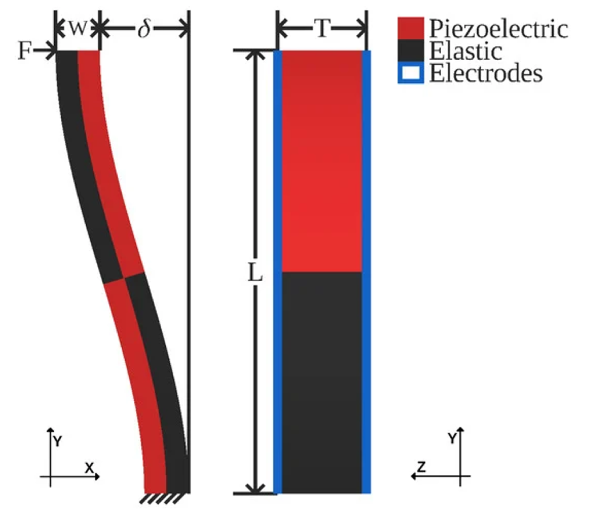
Figure 1.
S-drive design (Jones and Clark 2021).
Reduced-order models (ROMs) directly address these bottlenecks by approximating the full-order dynamics in a lower-dimensional representation. Classical ROMs like POD-Galerkin, Krylov subspace methods, and balanced truncation can be highly effective for linear or weakly nonlinear systems, yet they often struggle with nonlinear, hysteretic, and path-dependent solves without significant augmentation, and are often run concurrently on CPUs. On the other hand, modern neural surrogates can replace expensive PDE solvers with learned dynamics models that are highly optimized for GPUs, exploiting parallelism and millisecond-scale inference.
Much research, both recent and otherwise, has demonstrated the necessity for surrogate modeling. Notably, much promise has been shown in surrogate approaches for time-dependent PDEs and engineering systems, including non-intrusive, high-fidelity predictions of parameterized PDE solutions [5], LSTM-based acceleration in CAE design loops [6], and Gaussian-process surrogates for reliability analysis on complex engineering structures [7]. Furthermore, Meethal et al. (2022) demonstrated a surrogate-FEM middle ground, combining classical FEM with neural networks, creating well-performing and generalizable surrogate models for forward and inverse problems [8].
Despite these advances, modeling s-drive-based, tileable piezoelectric microactuators under time-varying electromechanical loading has received comparatively limited attention, particularly in the context of scalable microactuator-based systems simulation. In contrast to the aforementioned methods, we seek to develop a highly specialized and lightweight surrogate, suited for simulating many actuators where throughput is more important than single-actuator latency.
In this paper, we introduce a recurrent sequence-to-sequence surrogate that learns actuator dynamics from COMSOL-generated trajectories.
Throughout this work, the surrogate operates in a history-conditioned forecasting setting: given the most recent window of displacements together with the corresponding voltage/traction samples over that same history window, the model predicts the next H displacement futures as an open-loop rollout within the range of electromechanical conditions represented in the training data, enabling fast inference for long-horizon simulations and ensemble predictions.
Contributions:
- 1.
- A COMSOL-to-dataset pipeline that produces time-series trajectories spanning diverse voltage/traction waveforms.
- 2.
- A lightweight, GPU-optimized recursive sequence-to-sequence surrogate that predicts displacement rollouts from short history windows.
- 3.
- Evaluation on a holdout set showing strong fidelity in the main displacement channel and fast runtimes for a single actuator.
- 4.
- Evaluation of surrogate runtime scaling; performing batched inference across multiple GPUs, yielding predictions for millions of actuators.
Limitation
Because the surrogate is trained exclusively on finite element data, its accuracy is evaluated relative to the underlying FEA model and does not account for experimental or fabrication-induced discrepancies. Despite this, previous works have demonstrated permissible inaccuracies when comparing empirical actuator displacement to those yielded by FEM [9].

Table 1.
Comparison of ROM methods demonstrating their relation to governing equations, online complexity (for a single actuator), ability to generalize to unseen data, limitations, and common applications. The table taxonomy is as follows: number of layers, hidden units per layer, input feature dimension, number of query points, trainable parameter count, number of polynomial terms, inducing points, reduced-order-model state dimension
| Method | Governing Equations | Online Runtime Complexity | Generalization | Limitations | Examples and Applications |
|---|---|---|---|---|---|
| Long Short-Term Memory Networks (LSTMs) | No; data-driven, non-intrusive | ; (fixed architecture) | Moderate; typically strong within training envelope | Requires extensive and diverse data; training cost | Fluid Dynamics [10,11,12]; Aircraft landing load simulations [13] |
| Physics-Informed Neural Networks (PINNs) | No; residuals only needed for training | ; (fixed architecture) | Strong; physics residual helps with unseen inputs, and typically strong generalization within the training envelope | Training cost; retraining per problem | Non-Intrusive ROM of parameterized dynamic systems [14] |
| Polynomial Chaos Expansion (PCE) | No; statistical basis expansion | ; (fixed architecture) | Moderate; weak outside design/parameter space, stronger within | Curse of dimensionality | Dynamic analysis of structures with uncertainties [15] |
| Gaussian Process Regression (GPR) | No; nonparametric regression on data | (Sparse Variational GP) [16] | Moderate; Strong in-range, extrapolation trends to the kernel’s mean | Poor scaling with dataset size, curse of dimensionality, kernel sensitivity | ROM of geometrically nonlinear structures [17] |
| Proper Orthogonal Decomposition (POD-Galerkin) | Yes; projection onto basis | (Implicit); (Explicit) | Weak; limited to snapshot manifold, otherwise typically moderate-strong | Poor for highly nonlinear or hysteretic problems (without augmentation) | Microstructure modeling [18]; Blood-flow modeling [19] |
| Krylov Subspace Methods | Yes; projection of governing equations | (Implicit); (Explicit) | Moderate; typically strong for linear systems but weak under nonlinearity | Requires full system matrices; | Nodal analysis for MEMS simulations [20] |
| Balanced Truncation | Yes; needs full state-space matrices | (Implicit); (Explicit) | Typically Moderate | Can struggle with nonlinear dynamics (without augmentation) | Biological oscillator simulations [21] |
2. Methodology
The methodology described in this section defines a data-driven surrogate intended to approximate transient finite element simulations of a single s-drive actuator under prescribed electromechanical loading, rather than a first-principles physical model.
2.1. Actuator Design
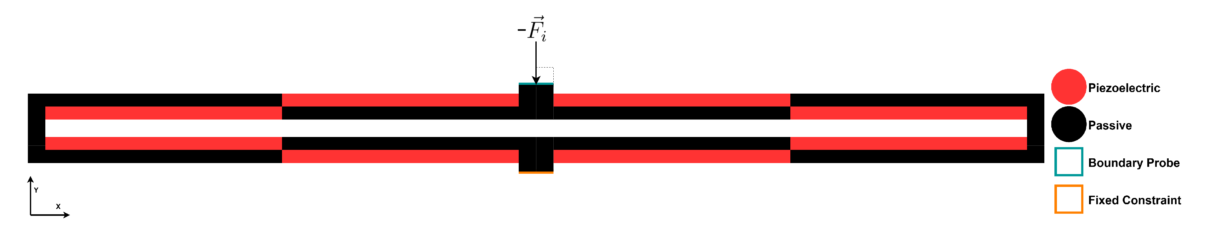
We instantiate our s-drive-based actuator in COMSOL Multiphysics 5.5, defining boundary conditions to excite coupled electromechanical dynamics while enabling consistent measurements of free-shuttle displacement:
- 1.
- Fixed constraint: the exterior face of the fixed shuttle on the -plane is clamped.
- 2.
- Traction + Displacement Probe: the opposing shuttle’s exterior face is subjected to time-varying traction load, and its displacement is recorded via a boundary probe during solves.
- 3.
- Voltage Terminals: a checkerboarded terminal pattern applies voltage on the top electrodes (), and all bottom () surfaces are grounded.
See Figure 4.
Figure 2.
S-drive-based actuator design (Jones and Clark 2021).
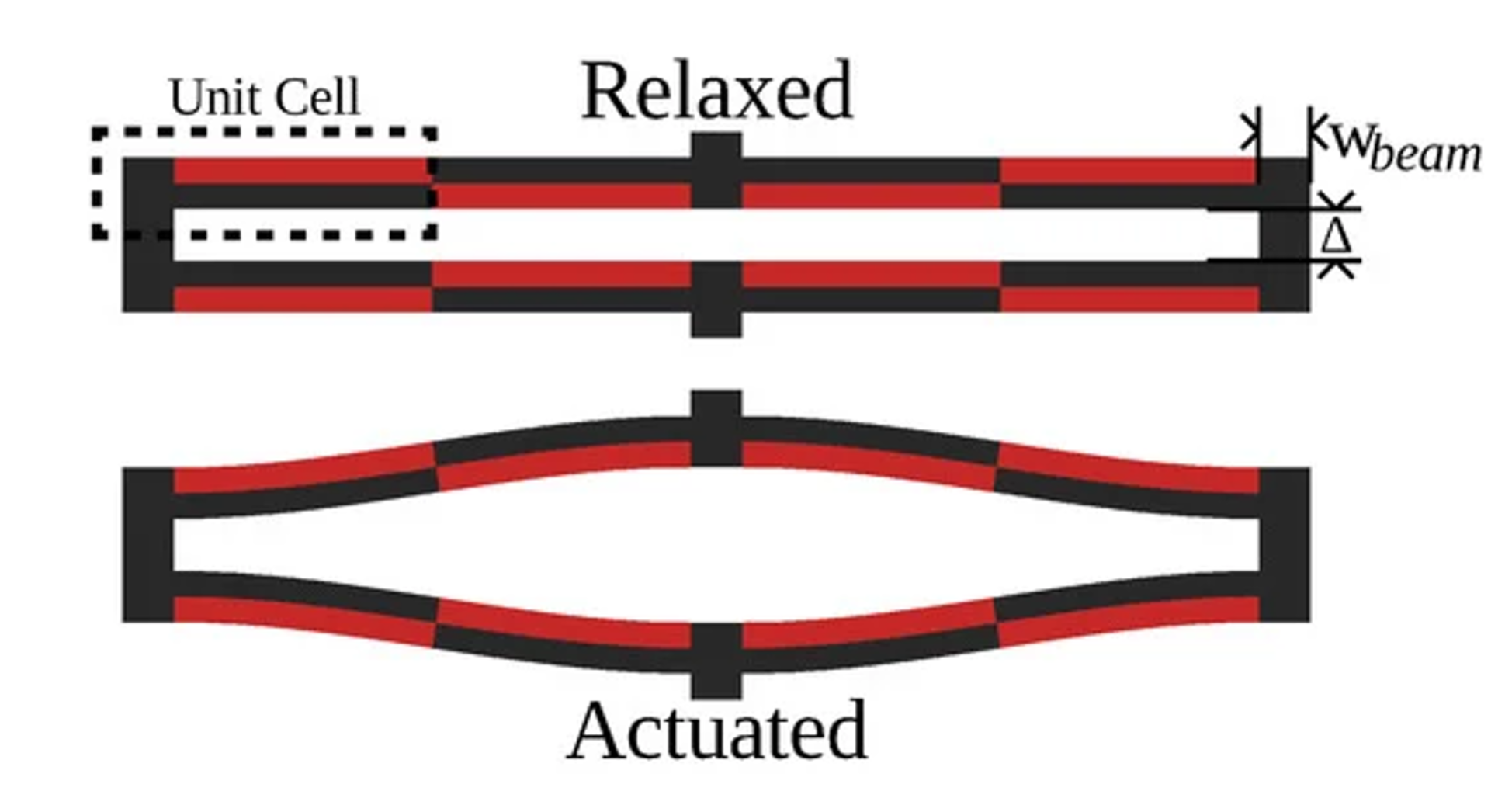
Figure 3.
Electrical Potential of our PZT-5H Actuator.
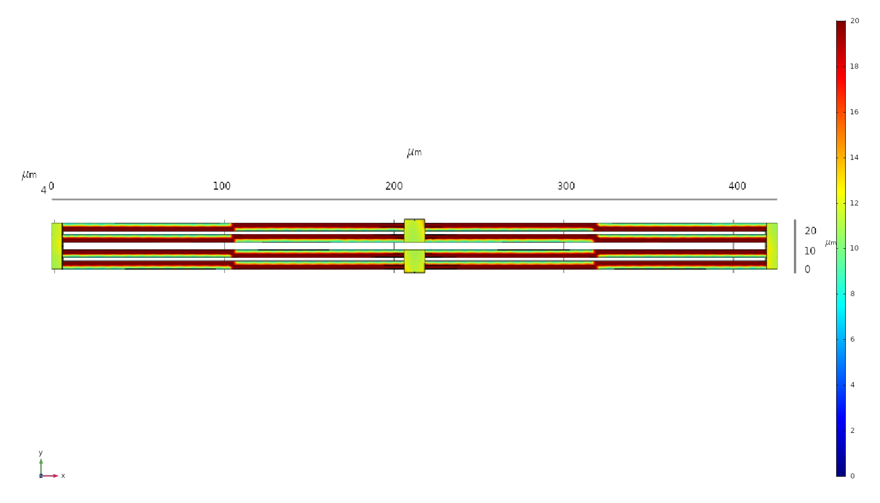
Figure 4.
Our PZT-5H Microactuator. Here is the traction we apply to the free-shuttle boundary at simulation step i. We define the boundary probe and fixed constraint as blue and orange, respectively. The actuator spans the bounding box [424 , 28 , 6 ].
Figure 4.
Our PZT-5H Microactuator. Here is the traction we apply to the free-shuttle boundary at simulation step i. We define the boundary probe and fixed constraint as blue and orange, respectively. The actuator spans the bounding box [424 , 28 , 6 ].
2.2. Material Selection
Prior work has validated s-drive actuator configurations in PZT-based devices via simulation, fabrication, and empirical tests [9]. We select PZT-5H due to its high piezoelectric coefficient (reported as [22]), making it a well-suited candidate for maximizing actuation. Despite its high piezoelectric response, it is important to note that lead-based ceramics like PZT-5H are highly toxic; thus, many biocompatible alternatives like PVDF and PVDF-TrFe have become particularly intriguing in recent years. However, due to their lower piezoelectric coefficients = 13-35 24-39 [23] and corresponding displacements, we select PZT-5H to demonstrate our surrogate’s ability to capture extreme nonlinearity and displacement.
For the s-drive, we are largely interested in higher values; measuring the stress produced orthogonally to the polarization axis. Unfortunately, is often much harder to measure experimentally; therefore, is more commonly used as a metric for deflection. Despite this, they have the following empirical relationship [24]
Importantly, all material properties are used solely within the finite element simulations that generate training data and are not explicitly enforced within the surrogate model.
2.3. Input Waveform Generation
To elicit a wide range of dynamic responses, we generate excitation waveforms in two stages: (i) 2500 ms of randomly sampled voltage V and traction MPa sampled at ms timesteps and (ii) 2500 ms of all permutations of the following families sampled at ms:
- Voltage waveforms (11 families): pseudorandom binary sequences (PRBS); square-pulse trains with random pulse widths; multi-sine signals (sum of five sinusoids with random frequencies and phases); logarithmic-frequency chirps; triangular waves with random frequency; sawtooth waves with random frequency; random telegraph (two-state) processes; sparse impulse trains (short high-amplitude pulses); hold-then-step waveforms; amplitude-modulated sine waves; and colored noise (white noise filtered by a moving-average filter).
- Force waveforms (12 families): pure sinusoidal waves with random frequency; linear ramps (increasing or decreasing); linear-frequency chirps; logarithmic-frequency chirps; piecewise-linear interpolations between randomly sampled anchor points; multi-sine signals (sum of five sinusoids); triangular waves with random frequency; sawtooth waves with random frequency; sparse impulse trains; hold-then-step waveforms; amplitude-modulated sine waves; and colored noise.
2.4. Simulation Hyperparameters
Due to the invariance in nonlinearity introduced by stochastically sampling our interpolation functions, different solver parameters were fixed for each waveform sampling method across all 4 transient runs:
- 1.
-
Gaussian Noise (ms),
- Time-Stepping Method: Backward Differentiation Formula (BDF) order 2;
- Relative Tolerance: ;
- Nonlinear Method: Constant (Newton);
- Nonlinear Method Maximum Iterations: 65;
- 2.
-
Waveform Family Combinations (ms)
- Time-Stepping Method: Backward Differentiation Formula (BDF) order 1;
- Relative Tolerance: ;
- Nonlinear Method: Constant (Newton);
- Nonlinear Method Maximum Iterations: 20;
For all runs, Jacobians were updated on every iteration, we used tolerance as our termination technique and the solution as the criterion.
The mesh is physics-controlled with a normal element size. COMSOL’s meshing procedure selected maximum element size , minimum element size , maximum element growth rate , curvature factor and, resolution of narrow regions as parameters. The resulting mesh consisted of 3881 domain elements, 3726 boundary elements, and 1654 edge elements yielding 34932 degrees of freedom.
2.5. Transient FEA Simulations and Data Collection
During transient solves, interpolation functions provide voltage inputs to terminals and traction inputs to the free-shuttle boundary, respectively. The interpolated traction is applied normally to the main face of the free shuttle, perturbing displacement in response to external mechanical stimuli. Then, the interpolated voltage is applied to the actuator’s terminals. These interpolated inputs span a large portion of the actuator’s operational envelope, giving the surrogate robust and diverse data. Here, the operational envelope refers to the range of voltage and traction inputs defined by the procedurally generated waveform families and bounds used in the finite element simulations, rather than the full space of physically realizable operating conditions. From our completed solves, we extract our boundary probe’s displacement components and the interpolated load values. Across 4 simulations, this yields time-indexed samples spanning the bulk of the actuator’s operational envelope.
2.6. Data Preprocessing
The raw dataset is exported from COMSOL for each transient simulation. Each simulation produces three displacement channels per timestep, denoted as and , corresponding to the and z displacement of the probe-surface. Furthermore, the simulation provides two interpolated electromechanical load function tables, representing the voltage load and external traction applied to the actuator during the transient solve for each timestep.
After parsing the exported COMSOL data, we construct the displacement matrix
and our feature vector, which appends the interpolation table.
2.6.1. Sliding-Window Sequence Generation
In initial prototypes, we mapped voltage-force and displacement histories to the displacement tuple at the next timestep. Despite its simplicity, this method incurs longer runtimes as often larger “strides” can be taken without excessive error. Enabling stride mechanisms, we train a multi-step surrogate that maps a short history of observed electromechanical states to a future displacement trajectory. Let L denote the encoder history length and H denote the prediction horizon. Our current training script fixes these to
We then construct a maximally-overlapping (stride-1) supervised dataset with examples:
for , this yields input tensors of shape and target tensors of shape .
During the rollout, the surrogate is evaluated in a history-conditioned forecasting setting: the encoder receives the most recent L samples of , while the decoder is driven by displacement (initialized with a zeroed start token and then fed its own predictions).
2.6.2. Training and Validation Splitting
After generating sliding windows, we split the data into training and validation sets with a split. The resulting shapes for our training and validation sets are:
- . This array represents 449883 samples of displacement/electromechanical loading histories of length 32, representing of time series of approximately seconds.
- . This array represents 449883 samples of displacement futures of length 100, representing of time series of approximately seconds.
- . This array represents 49988 samples of displacement/electromechanical loading histories of length 32, representing of time series of approximately seconds.
- . This array represents 49988 samples of displacement futures of length 100, representing of time series of approximately seconds.
Limitation
Training and validation splits are performed after sliding-window generation; consequently, validation windows may be temporally adjacent to training windows and share overlapping history; the reported validation metrics therefore may only reflect interpolation performance within the simulated input space rather than trajectory-level extrapolation.
2.6.3. Feature Standardization
To stabilize optimization and prevent single-channel domination on the gradient, all five input vectors are standardized using global mean and standard deviation computed over the entire concatenated feature stream:
with in our implementation. The standardized windows are then
Standardization is applied independently to each input and output channel using global statistics; consequently, channels with small physical variance are weighted equally during training and may exhibit large relative error or low despite having small absolute displacement errors.
2.7. Surrogate Model Architecture
The goal is to learn a fast surrogate for the actuator’s transient response conditioned on a recent history of electromechanical states. Contrary to learning a single future state, we predict a future displacement trajectory. This is crucial for efficient rollouts on numerous actuators because predicting H steps at once amortizes the model’s overhead. Given our standardized history window , our sequence to sequence surrogate produces
where each row is a predicted displacement vector. Our lightweight implementation is well-suited for massive parallel instantiation on GPU hardware.
Our model uses Gated Recurrent Unit (GRU) layers to capture temporal dependencies. Introduced in 2014 by Kyunghyun Cho, the GRU architecture uses update and reset gates to control information flow with fewer parameters than its counterparts; LSTMs and Transformers [25].
- 1.
- a 2-layer GRU encoder that compresses the L-step input history into a stacked hidden state;
- 2.
- a 2-layer GRU decoder that autoregressively generates H future displacement vectors conditioned on the encoder’s hidden state;
- 3.
- and finally, a linear projection that maps the decoder hidden vectors to displacement outputs.
We set the hidden size to 64, and the decoder input dimension is fixed to the output dimension 3.
Dropout and Regularization
Three distinct regularization mechanisms appear in the model definition: (i) input dropout applied to encoder inputs with probability ; (ii) recurrent-layer dropout internal to PyTorch’s stacked GRU layers with probability between layers; and (iii) dropout applied to decoder outputs before projection with probability . During training, we also inject Gaussian noise into the standardized input windows.
2.7.1. GRU Encoder
Let denote the standardized encoder input sequence, where . We first apply feature dropout to the encoder inputs
and then apply additive Gaussian noise to the standardized windows with standard deviation :
The encoder stacks 2 GRU layers. For completeness, the GRU updates at a time t for a single layer are
In our stacked architecture, the input to layer ℓ is the hidden sequence produced by . The encoder returns the final hidden state for all layers,
which is used to initialize the decoder hidden state.
2.7.2. GRU Decoder
The decoder is a stacked GRU with the same number of layers and hidden sizes as the encoder. Unlike the encoder, the decoder input at each step is a predicted displacement vector in . The model uses a fixed start of sequence token equal to the zero displacement vector
Conditioned on the encoder hidden state, the decoder generates a rollout autoregressively for :
where is the decoder output. Before mapping to displacements, dropout is applied to :
and the projection
yields our displacement prediction . Then, finally, the decoder input is set to its own prediction:
Stacking the predictions yields .
2.7.3. Loss Function and Optimization
The mean-squared error over all horizon steps and the displacement channels’ loss function
encourages the model to minimize the difference between displacement channels from its prediction and our training set.
2.8. Training Hyperparameters
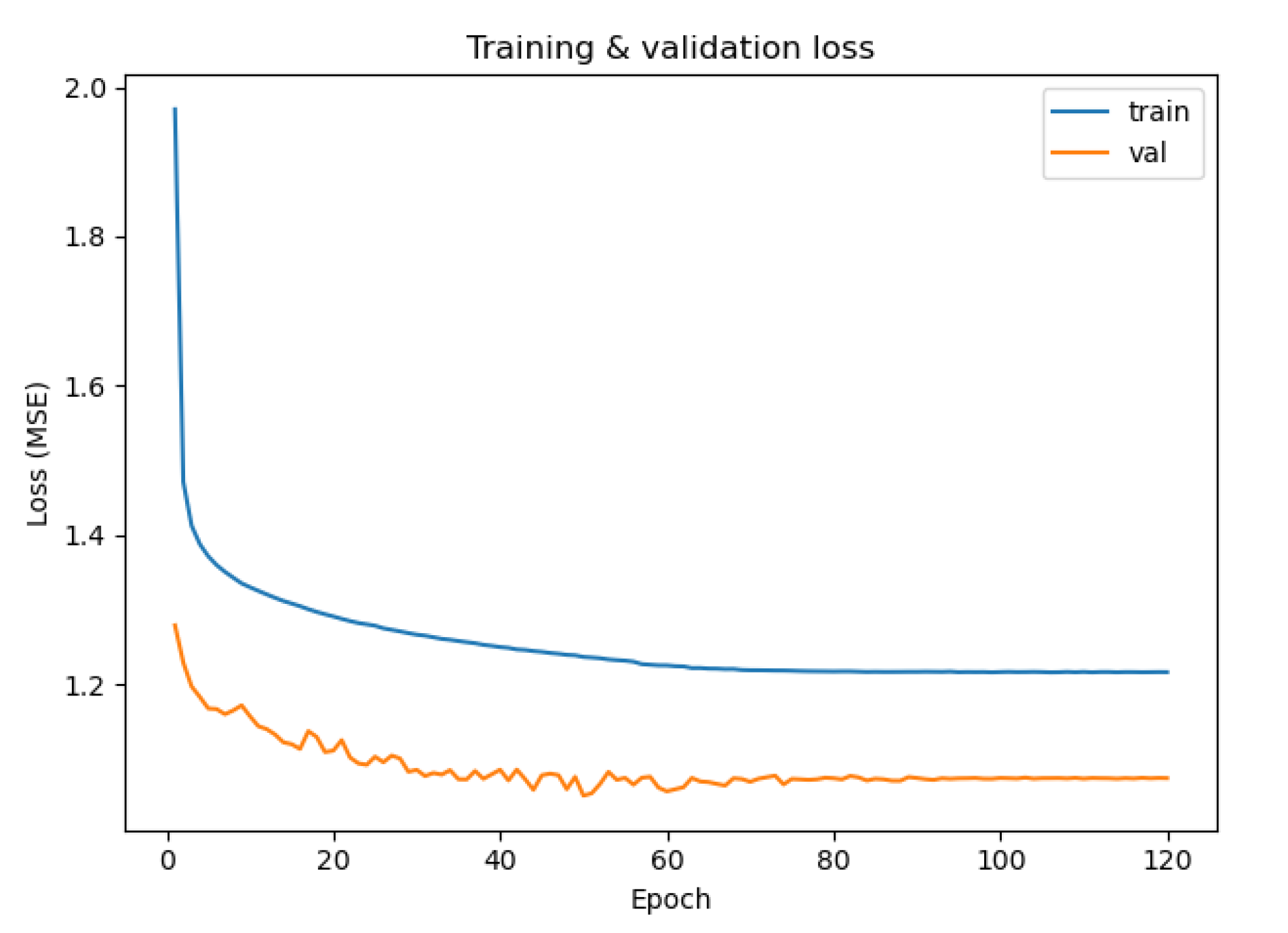
We train the surrogate using the Adam optimizer [26] with learning rate and minimize the horizon-averaged MSE in Equaton (18). Training uses automatic mixed precision (AMP) with gradient scaling, global-norm gradient clipping (), and additive Gaussian noise applied to inputs with standard deviation to standardized input windows. A ReduceLROnPlateau scheduler monitors validation loss and decays the learning rate by a factor of after 5 epochs without improvement, with a learning rate floor of . Model training concludes after 120 epochs, retaining the checkpoint with the lowest validation loss using a fixed random seed.
Figure 5.
Surrogate model training vs. validation loss during optimization.
3. Results
3.1. Single-Surrogate Performance
All results in this section evaluate surrogate predictions relative to held-out finite element simulations and are intended to assess fidelity and computational efficiency with respect to transient FEA.
Model training terminated after 120 epochs, reaching on a subset of the training set and on the validation set. The coefficient of determination () is reported for completeness but should be interpreted with caution for the u and w displacement channels. measures how much of the variation in the data you explain, not how big the error is. These channels exhibit extremely small physical variation in the finite element data, such that even very small absolute prediction errors can produce large negative values. For these channels, absolute error metrics provide a more meaningful indication of surrogate accuracy than variance-normalized measures.
Despite relatively strong metrics across all horizon windows, there are significant discrepancies between performance across the three displacement channels (see Table 2). The explanation for this inconsistency is simple; the actuator produces significant deflection in y-direction , whereas its out of plane deflections are limited to nanometers (see Table 3). Because s-drive actuation is designed to produce large in-plane displacement, performance in the v direction is the primary engineering metric of interest, while u and w displacements are secondary and remain near zero under normal operation. Correcting out-of-plane inaccuracy can be easily achieved by (i) introducing a weighted-sum loss function or (ii) applying torsional or oblique traction to encourage diverse out-of-plane deflections during FEA.
Note that our tolerance-based stride selection is an oracle benchmarking mechanism because it uses the held-out FEA displacement to choose ; in deployment, stride selection must be estimated without access to ground truth (either through a learned mechanism or set constant). The tolerance-based stride mechanism simply serves as a demonstration of how throughput can be maximized by exploiting the autoregressive nature of our architecture. Importantly, we observe that differing stride selections introduce significant changes in simulation runtime and accuracy (see Figure 6 and Figure 7). We run our surrogate across various stride lengths across the validation set. We execute our runtime evaluation script using the SLURM workload manager with 64 cores on two Intel(R) Xeon(R) Platinum 8168 CPUs @2.70GHz, an NVIDIA Tesla V100 with of VRAM, and of memory.
We observed the following noteworthy results:
- 1.
- Longest time to completion at seconds.
- 2.
- Shortest time to completion at seconds.
- 3.
- Highest u-channel accuracy: .
- 4.
- Highest v-channel accuracy: .
- 5.
- Highest w-channel accuracy: .
Apart from channel-wise accuracy, we test how runtime varies across all the valid stride lengths . From our results, we observe a monotonically decreasing curve with a steep initial drop for small horizon distances in Figure 7. Thus, our surrogate is suited for extremely high fidelity solves, producing up to for v-channel displacement, well within the empirically observed accuracy discontinuity between COMSOL FEA on PZT s-drives and the experimental validation () [9]. Because the surrogate is trained and evaluated exclusively on finite element simulations, its fidelity reflects consistency with the numerical model and does not include experimental uncertainties or fabrication effects. Furthermore, lower fidelity solves yield lower accuracy but with orders-of-magnitude speedups.
3.2. Multi-Surrogate Runtime Performance
Instantiating our model into a multi-surrogate setup, we push a single surrogate into both of our NVIDIA H100’s with of VRAM each, of 4800 MT/s memory, and 64 cores from -core Intel Xeon Platinums @Ghz. Concretely, we replicate the trained sequence-to-sequence forecaster once per GPU and execute inference using BF16 autocast on CUDA with TF32-enabled matrix multiplies. Each replica processes a batched set of actuator states in parallel, while a CPU dispatcher assigns shards to devices so that both GPUs remain fully saturated throughout the rollouts. Our end-to-end evaluation script reports (i) total wall-clock time for a full validation set rollout and (ii) effective throughput (samples/second), where a sample denotes one surrogate state advanced by one rollout window.
3.2.1. Tolerance-Driven Stride Selection
To reduce redundant evaluations on horizon rollouts, we reuse the model’s multi-step forecast in chunks. Concretely, given a window prediction for sample i, we compute a per-step RMSE
Given a user specified tolerance (instantiated as in our implementation), we select a per-sample stride
We then advance the rolling input buffer by inserting the next k normalized predicted displacement steps and shifting the history window forward. For a rollout of length N, the number of required windows is , therefore, a smaller k increases the number of required windows and runtime.
3.2.2. Scaling Behavior: Throughput and Simulation Runtime
To characterize scaling, we sweep the batch size over powers of two:
Figure 8 and Figure 9 summarize the results. Sequence throughput rapidly increases with batch size as kernel launch overhead decreases and GPU utilization improves: from samples/s at batch size 2 to samples/s by batch size 2048, and reaching samples/s by batch size (16384), a net speedup of . Beyond , performance plateaus in the range samples/s, with only marginal gains from further increases in batch size. Practically, this indicates that once both H100s are saturated, additional batching primarily increases memory costs without meaningful improvement of throughput.
The batch-size sweep exhibits a bi-modal runtime profile because our benchmark couples workload size and rollout length to the dynamically chosen stride length. In each run, the total number of simulated surrogates scales as , while the rollout advances in chunks of length k selected by the tolerance mechanism. Because the end-to-end runtime is easily approximated by , the runtime becomes piecewise and can change abruptly even when the median stride differs by only a few points. For example, once S saturates at the full validation set (), a stride of , requires windows, whereas a modest reduction to increases this to 24994 windows (a increase), and the degenerate case forces windows, producing a sharp wall-clock spike despite similar per-window GPU throughput. Conversely, where the tolerance mechanism permits larger strides, e.g., , the same rollout only requires windows, yielding an order-of-magnitude reduction in total runtime, albeit with significant error. Despite this great variance, there is still a strong correlation between batch size and runtime. Importantly, there is no “one size fits all” stride selection method. On the surface, this seems like a limitation; however, this framework can be tailored both for extremely large-scale, high-throughput simulations involving millions of actuators and for small-scale analyses that closely reproduce transient finite element responses under tighter stride or tolerance settings.
4. Discussion
The following discussion interprets the results in terms of fidelity to transient finite element simulations and the computational tradeoffs enabled by data-driven surrogate modeling.
Figure 10.
S-drive-based muscle design (Jones and Clark 2021).
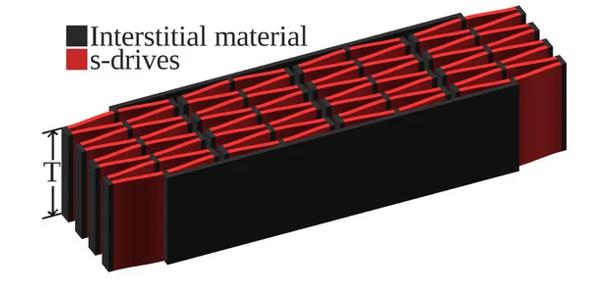
Figure 11.
Visualization of an actuator array () alongside a U.S. penny for scale. Full video available at https://youtu.be/eyIukrxz_YM?si=1i4F-cFcoKplFSmO.
Figure 11.
Visualization of an actuator array () alongside a U.S. penny for scale. Full video available at https://youtu.be/eyIukrxz_YM?si=1i4F-cFcoKplFSmO.
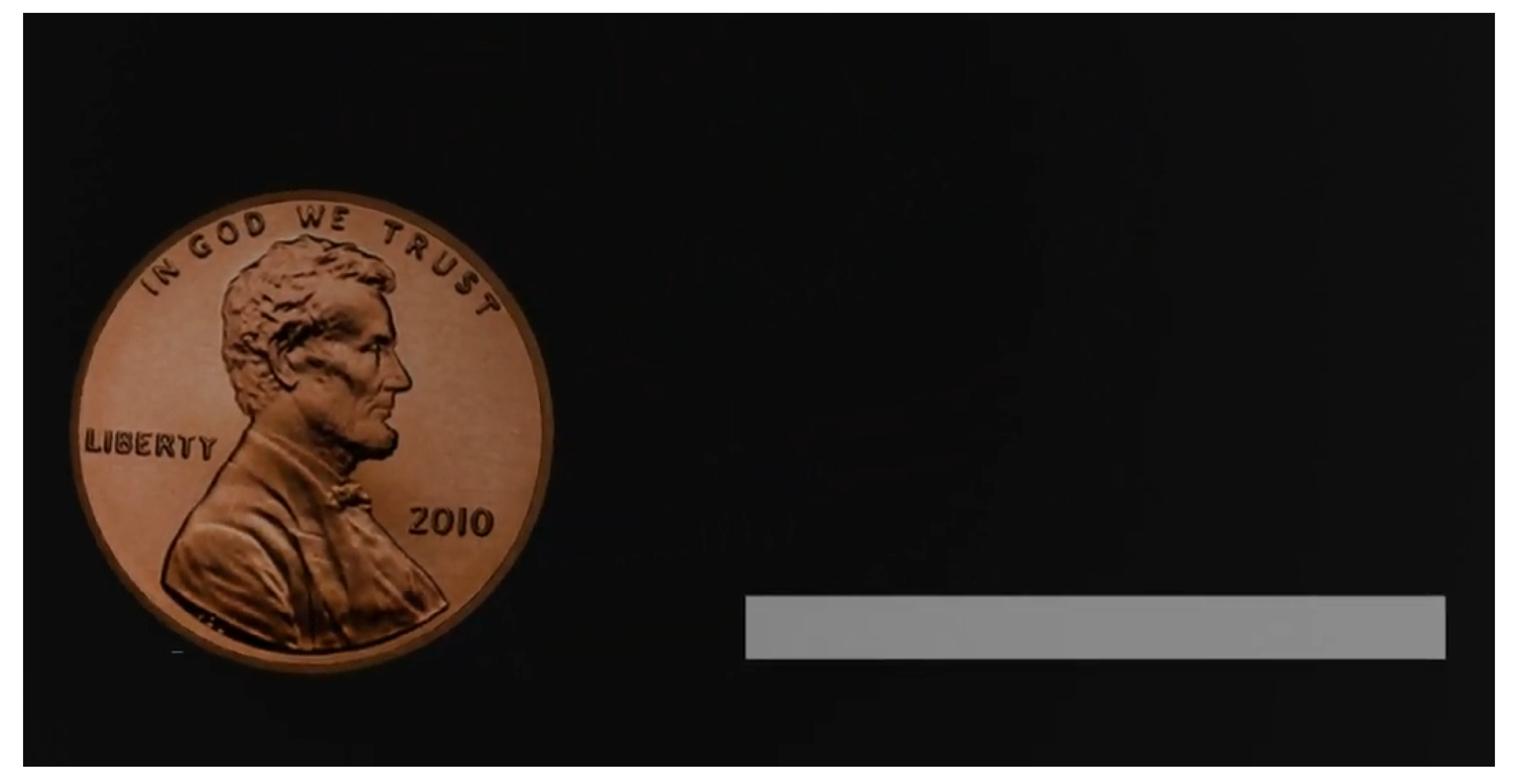
Despite the imperfect performance on u and w displacement channels, the surrogate’s millisecond-scale inference enables substantial reductions in simulation time relative to transient finite element analysis. Using GPU hardware, we can now predict the dynamic response of over 67 million independent actuators in minutes, whereas traditional PDE solvers like COMSOL are simply unable to solve or even construct such systems. Despite this, FEA tools like COMSOL and ANSYS remain invaluable due to their ease-of-use, non-intrusiveness, and grounding in constitutive equations. In summary, by trading reduced fidelity to finite element predictions for substantial gains in computational throughput and parallelizability, the surrogate unlocks a range of tasks that were previously infeasible with direct finite element analysis.
- Model-Based Reinforcement Learning (MBRL) Direct policy optimization on finite-element models is computationally prohibitive: single transient FEA simulations can take minutes, hours, or even days depending on model size and parameters, making the millions of interactions required by reinforcement learning infeasible. Despite the poor runtime with these models, they are greatly limited by how many degrees of freedom they need to solve, limiting them to smaller-scale assemblies. In contrast, our surrogate can serve as a component-wise dynamics model in an MBRL loop, making predictions in milliseconds, reducing runtimes significantly, and allowing for large-scale assemblies. This dramatic speedup, combined with a highly portable neural network, makes policy optimization practical for piezoelectric microactuator-based systems.
-
Architecture Search Parker et al. demonstrated the feasibility of architecture search in piezoelectric microactuator design, performing systematic sweeps of electrode width, passive-region width, and layer thickness via finite-element analysis to identify geometries that maximize in-plane deflection [27]. Their study highlights the viability and importance of autonomous exploration of geometry search spaces on piezoelectric microactuator-based systems. While focusing on single s-drive optimization, a full-actuator surrogate could be used to accelerate optimization on actuator assemblies.Cheney et al. demonstrated that compositional-pattern-producing networks (CPPNs) combined with a library of various materials allow for the evolution of optimized morphologies for trivial tasks such as locomotion [28]. In theory, a similar approach could be applied by leveraging this surrogate framework, creating optimal geometries of microactuator-based robots for specific tasks.
Due to the difficulty in manufacturing high-fidelity s-drive microactuators, the surrogate is trained and evaluated exclusively on finite element data, its fidelity reflects consistency with the underlying numerical model and does not capture experimental uncertainties or fabrication-induced variability.
5. Conclusions
We have presented a data-driven surrogate modeling framework for replacing transient finite element simulations with a surrogate that leverages stacked gated recurrent units to predict boundary displacements of piezoelectric microactuators with millisecond-scale latency. By generating a two-stage waveform library and simulating each sequence with high-fidelity COMSOL FEA on a PZT-5H actuator, we compiled a diverse dataset of half a million time steps covering the device’s dynamic envelope. Our GRU model, trained on 32-step sliding windows of normalized displacements and interpolated load values, achieves millisecond-scale inference per rollout window when reproducing transient finite element responses and is easily parallelizable on GPU hardware.
Future work will focus on mechanical coupling, empirical validation, and realizing intelligent s-drive-based actuator systems. Through reinforcement learning and genetic search, we aim to create intelligent microrobots, blurring the lines between artificial and biological systems. Before this, much work needs to be done on streamlining the fabrication process of these microstructures and designing surrogate frameworks that perform as closely as possible to their real-world counterparts.
Author Contributions
Conceptualization, J.S. and J.C.; methodology, J.S.; software, J.S. and J.C.; validation, J.S.; formal analysis, J.S.; investigation, J.S.; resources, J.C.; data curation, J.S.; writing—original draft preparation, J.S. and D.T.; writing—review and editing, J.S., J.C. and D.T.; visualization, J.S.; supervision, J.C.; project administration, J.S.; CRediT taxonomy
Funding
This research received no external funding
Data Availability Statement: Data available in a publicly accessible repository
FEA dataset, surrogate training and batched inference scripts are available on Github at https://github.com/John-Scumniotales/PZT-5H-Microactuator-Surrogate-Modelling-Scripts. Due to model size, COMSOL files are available only upon request.
Acknowledgments
The authors gratefully acknowledge the use of HPC nodes managed by the Oregon State University College of Engineering. We thank COE IT for maintaining these systems, enabling rapid model training and simulation workflows. We thank “Yanez Designs” for the 3D penny model used in Figure 11.
References
- Rugar, D.; Hansma, P. Atomic Force Microscopy. Physics Today 1990, 43, 23–30. [Google Scholar] [CrossRef]
- Bußmann, A.B.; Durasiewicz, C.P.; Kibler, S.H.A.; Wald, C.K. Piezoelectric titanium based microfluidic pump and valves for implantable medical applications. Sensors and Actuators A: Physical 2021, 323, 112649. [Google Scholar] [CrossRef]
- Mangi, M.A.; Elahi, H.; Ali, A.; Jabbar, H.; Aqeel, A.B.; Farrukh, A.; Bibi, S.; Altabey, W.A.; Kouritem, S.A.; Noori, M. Applications of piezoelectric-based sensors, actuators, and energy harvesters. Sensors and Actuators Reports 2025, 9, 100302. [Google Scholar] [CrossRef]
- Extremely Large Deflection Actuators for Translation or Rotation, Vol. ASME International Mechanical Engineering Congress and Exposition, 2012; : Micro- and Nano-Systems Engineering and Packaging, Parts A and B; Volume 9. [CrossRef]
- Nikolopoulos, S.; Kalogeris, I.; Papadopoulos, V. Non-intrusive Surrogate Modeling for Parametrized Time-dependent PDEs using Convolutional Autoencoders. arXiv 2021, arXiv:math. [Google Scholar]
- Kohar, C.P.; Greve, L.; Eller, T.K.; Connolly, D.S.; Inal, K. A machine learning framework for accelerating the design process using CAE simulations: An application to finite element analysis in structural crashworthiness. Computer Methods in Applied Mechanics and Engineering 2021, 385, 114008. [Google Scholar] [CrossRef]
- Su, G.; Peng, L.; Hu, L. A Gaussian process-based dynamic surrogate model for complex engineering structural reliability analysis. Structural Safety 2017, 68, 97–109. [Google Scholar] [CrossRef]
- Meethal, R.E.; Obst, B.; Khalil, M.; Ghantasala, A.; Kodakkal, A.; Bletzinger, K.U.; Wüchner, R. Finite Element Method-enhanced Neural Network for Forward and Inverse Problems. 2023. [Google Scholar] [CrossRef]
- Chigullapalli, A. Modeling and Validation of S-Drive: A Nestable Piezoelectric Actuator. 2014. [Google Scholar]
- Mohan, A.T.; Gaitonde, D.V. A Deep Learning based Approach to Reduced Order Modeling for Turbulent Flow Control using LSTM Neural Networks. arXiv 2018, arXiv:1804.09269. [Google Scholar] [CrossRef]
- Halder, R.; Damodaran, M.; Cheong, K.B. Deep Learning-Driven Nonlinear Reduced-Order Models for Predicting Wave-Structure Interaction. arXiv 2023, arXiv:physics.flu. [Google Scholar] [CrossRef]
- Ahmed, S.E.; San, O.; Rasheed, A.; Iliescu, T. A long short-term memory embedding for hybrid uplifted reduced order models. Physica D: Nonlinear Phenomena 2020, 409, 132471. [Google Scholar] [CrossRef]
- Lazzara, M.; Chevalier, M.; Colombo, M.; Garay Garcia, J.; Lapeyre, C.; Teste, O. Surrogate modelling for an aircraft dynamic landing loads simulation using an LSTM AutoEncoder-based dimensionality reduction approach. Aerospace Science and Technology 2022, 126, 107629. [Google Scholar] [CrossRef]
- Dave, H.; Cotteleer, L.; Parente, A. Physics-informed non-intrusive reduced-order modeling of parameterized dynamical systems. Computer Methods in Applied Mechanics and Engineering 2025, 443, 118045. [Google Scholar] [CrossRef]
- Yang, J.; Faverjon, B.; Peters, H.; Kessissoglou, N. Application of Polynomial Chaos Expansion and Model Order Reduction for Dynamic Analysis of Structures with Uncertainties. Procedia IUTAM;Dynamical Analysis of Multibody Systems with Design Uncertainties 2015, 13, 63–70. [Google Scholar] [CrossRef]
- Hensman, J.; Fusi, N.; Lawrence, N.D. Gaussian Processes for Big Data. arXiv 2013, arXiv:1309.6835. [Google Scholar] [CrossRef]
- Park, K.; Allen, M.S. A Gaussian process regression reduced order model for geometrically nonlinear structures. Mechanical Systems and Signal Processing 2023, 184, 109720. [Google Scholar] [CrossRef]
- Gobat, G.; Opreni, A.; Fresca, S.; Manzoni, A.; Frangi, A. Reduced order modeling of nonlinear microstructures through Proper Orthogonal Decomposition. Mechanical Systems and Signal Processing 2022, 171, 108864. [Google Scholar] [CrossRef]
- Chatpattanasiri, C.; Franzetti, G.; Bonfanti, M.; Diaz-Zuccarini, V.; Balabani, S. Towards Reduced Order Models via Robust Proper Orthogonal Decomposition to capture personalised aortic haemodynamics. Journal of Biomechanics 2023, 158, 111759. [Google Scholar] [CrossRef]
- Bai, Z.; Bindel, D.; Clark, J.; Demmel, J.; Pister, K.; Zhou, N. New numerical techniques and tools in SUGAR for 3D MEMS simulation. 2001. [Google Scholar]
- Padoan, A.; Forni, F.; Sepulchre, R. Balanced truncation for model reduction of biological oscillators. Biological Cybernetics 2021, 115. [Google Scholar] [CrossRef]
- Hooker, M.W. Properties of PZT-Based Piezoelectric Ceramics Between -150 and 250 C 1998.
- Bhadwal, N.; Ben Mrad, R.; Behdinan, K. Review of Piezoelectric Properties and Power Output of PVDF and Copolymer-Based Piezoelectric Nanogenerators. Nanomaterials 2023, 13. [Google Scholar] [CrossRef]
- Li, J.F. Lead-free piezoelectric materials; Wiley-VCH: Weinheim, 2021. [Google Scholar]
- Chung, J.; Gülçehre, Ç.; Cho, K.; Bengio, Y. Empirical Evaluation of Gated Recurrent Neural Networks on Sequence Modeling. CoRR 2014, abs/1412.3555, 1412.3555. [Google Scholar]
- Kingma, D.P.; Ba, J. Adam: A Method for Stochastic Optimization. arXiv 2017, arXiv:1412.6980. [Google Scholar] [CrossRef]
- Megginson, P.; Clark, J.; Clarson, R. Optimizing the Electrode Geometry of an In-Plane Unimorph Piezoelectric Microactuator for Maximum Deflection. Modelling 2024, 5, 1084–1100. [Google Scholar] [CrossRef]
- Cheney, N.; MacCurdy, R.; Clune, J.; Lipson, H. Unshackling Evolution: Evolving Soft Robots with Multiple Materials and a Powerful Generative Encoding. 2013. [Google Scholar] [CrossRef]
Figure 6.
displacement values () measured in microns predicted from our surrogate on the validation set with stride values and 32 ordered from left to right.
Figure 6.
displacement values () measured in microns predicted from our surrogate on the validation set with stride values and 32 ordered from left to right.
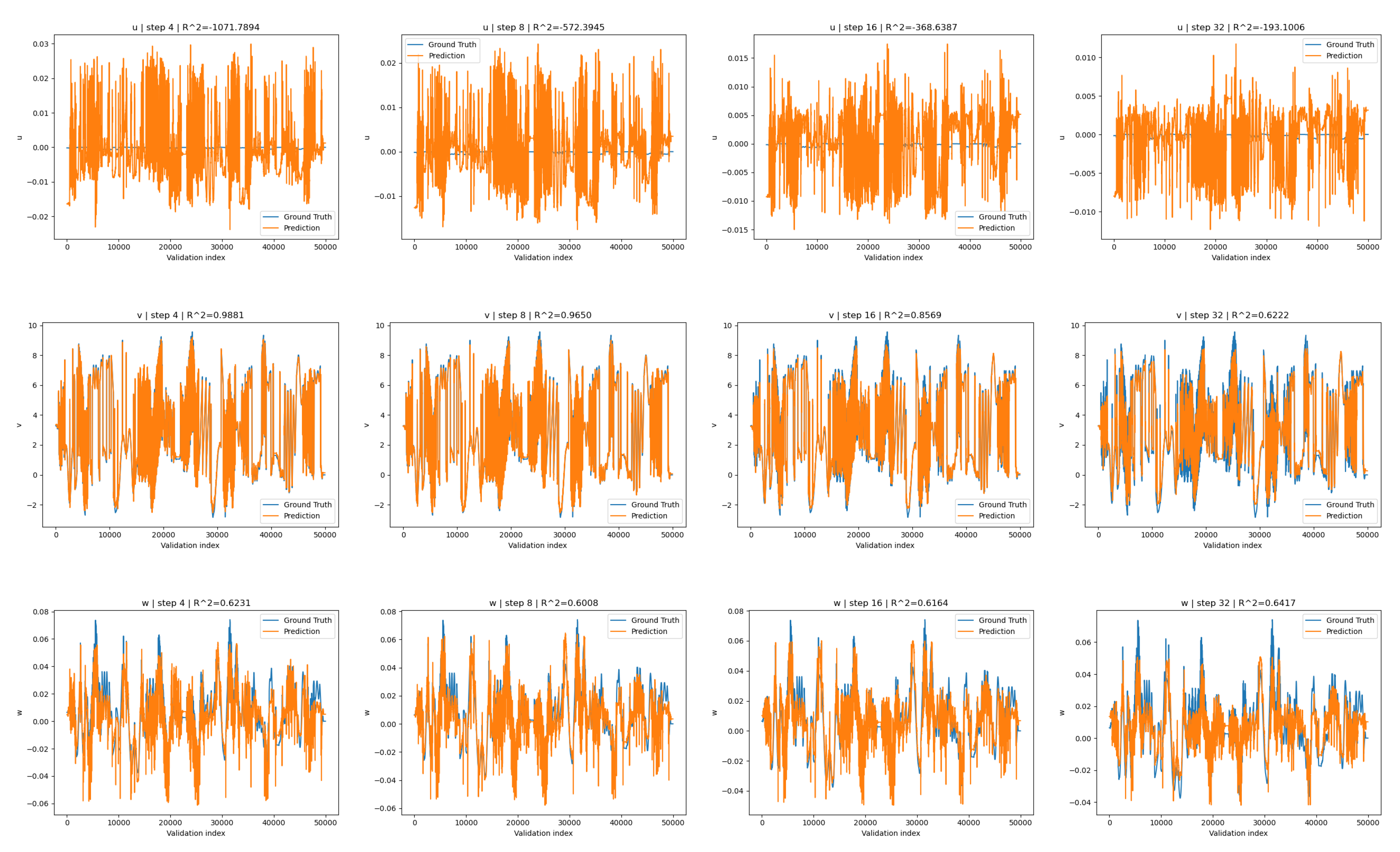
Figure 7.
Surrogate-evaluation runtime (ms) vs. horizon length.
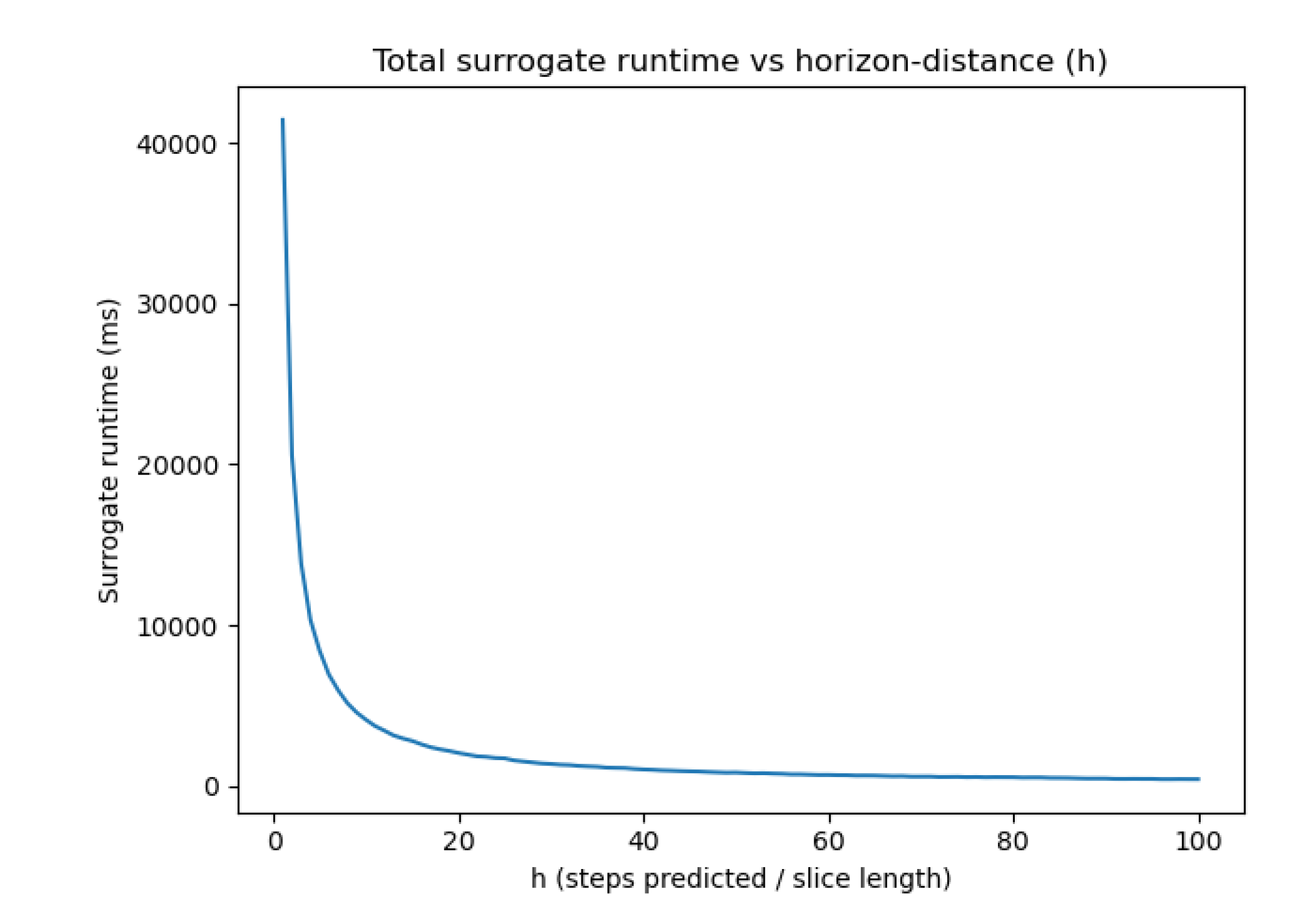
Figure 8.
Batch size vs simulation runtime on 49988 validation samples.
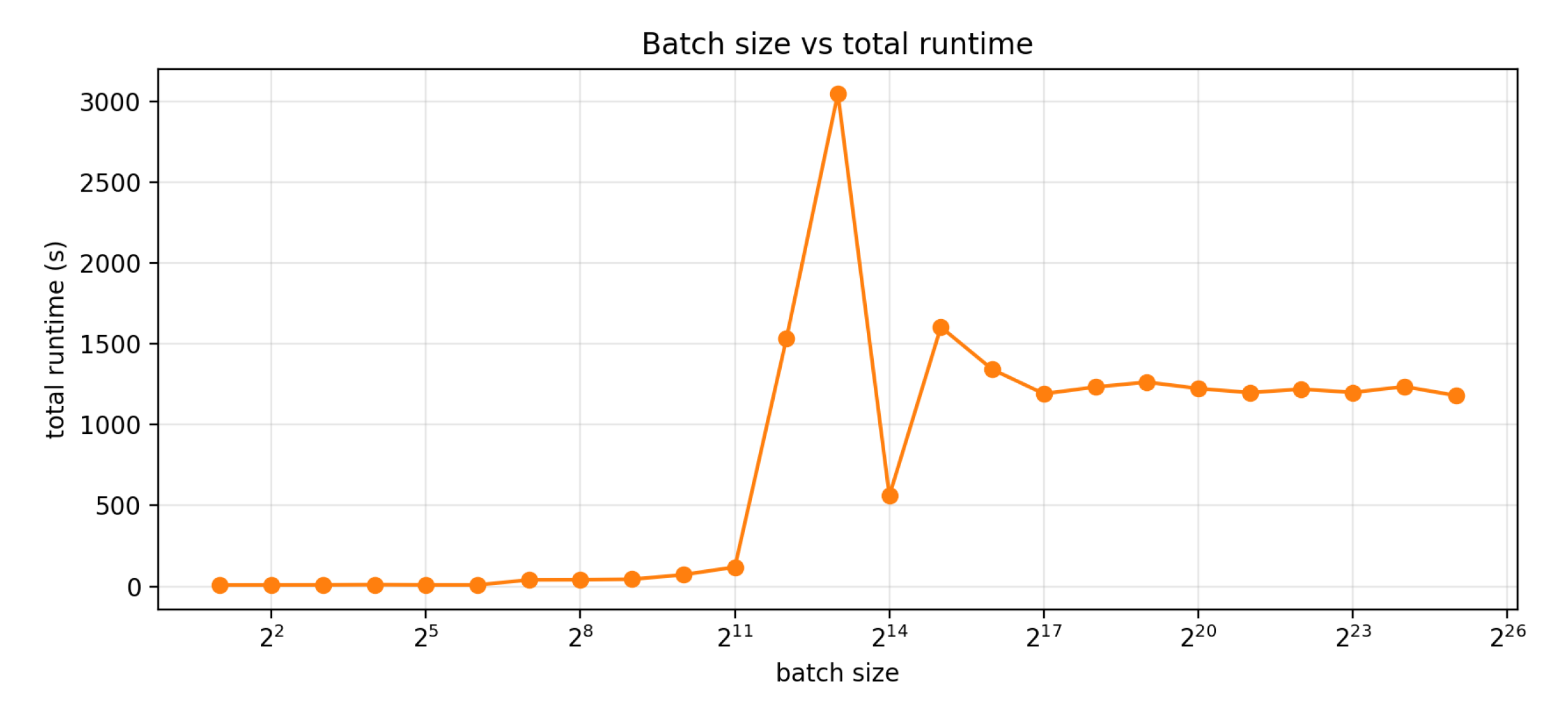
Figure 9.
Batch size vs sample throughput on 49988 validation samples.
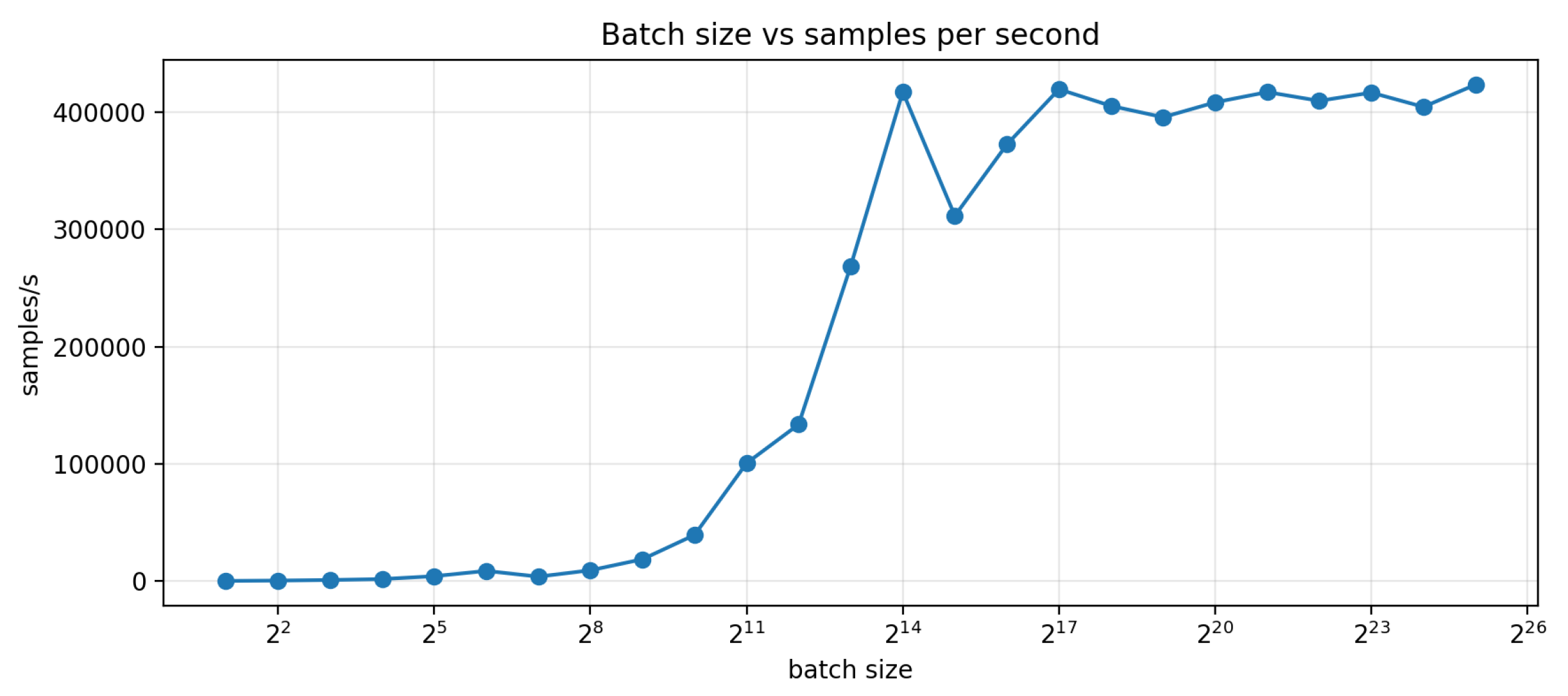
Table 2.
Horizon-offset Accuracy Metrics.
| Forecast offset | |||||||||
|---|---|---|---|---|---|---|---|---|---|
| 1 | -2529.5193 | 0.9919 | 0.4015 | 0.000131 | 0.064094 | 0.000222 | 13.177775 | 0.020391 | 0.133553 |
| 2 | -1708.5314 | 0.9927 | 0.5391 | 0.000089 | 0.057791 | 0.000171 | 10.831262 | 0.019363 | 0.117193 |
| 4 | -1071.7894 | 0.9881 | 0.6231 | 0.000056 | 0.094217 | 0.000140 | 8.580334 | 0.024723 | 0.105975 |
| 8 | -572.3945 | 0.9650 | 0.6008 | 0.000030 | 0.276449 | 0.000148 | 6.273164 | 0.042349 | 0.109068 |
| 16 | -368.6387 | 0.8569 | 0.6164 | 0.000019 | 1.132312 | 0.000142 | 5.037027 | 0.085707 | 0.106912 |
| 32 | -193.1006 | 0.6222 | 0.6417 | 0.000010 | 2.989624 | 0.000133 | 3.650484 | 0.139266 | 0.103341 |
| 64 | -154.2807 | 0.4955 | 0.5109 | 0.000008 | 3.994171 | 0.000182 | 3.265867 | 0.160972 | 0.120734 |
| 100 | -174.1376 | 0.4016 | 0.3725 | 0.000009 | 4.741710 | 0.000233 | 3.469326 | 0.175389 | 0.136763 |
Table 3.
COMSOL FEA free-shuttle boundary displacement data.
| Channel | Min | Max | Mean |
|---|---|---|---|
| u | |||
| v | |||
| w |
Disclaimer/Publisher’s Note: The statements, opinions and data contained in all publications are solely those of the individual author(s) and contributor(s) and not of MDPI and/or the editor(s). MDPI and/or the editor(s) disclaim responsibility for any injury to people or property resulting from any ideas, methods, instructions or products referred to in the content. |
© 2026 by the authors. Licensee MDPI, Basel, Switzerland. This article is an open access article distributed under the terms and conditions of the Creative Commons Attribution (CC BY) license (http://creativecommons.org/licenses/by/4.0/).
Copyright: This open access article is published under a Creative Commons CC BY 4.0 license, which permit the free download, distribution, and reuse, provided that the author and preprint are cited in any reuse.


