
Submitted:
18 July 2025
Posted:
21 July 2025
You are already at the latest version
Abstract
Hybrid modeling aims to combine physical and data-driven models to increase simulation accuracy without losing physical interpretability. In the context of dynamic mechanical systems, this enables the compensation of modeling inaccuracies that arise from simplifications, missing effects, or uncertain parameters. In this work, a hybrid model is used as a starting point, in which the discrepancy between simulation and measurement is learned and compensated by a data-driven correction element. To integrate such models into commercial multibody system (MBS) software like MSC Adams and Simpack, the formulation is adapted to operate directly on the force level. This allows implementation via standard co-simulation interfaces without modifying the system’s differential equations or solvers. The method is demonstrated using a single-mass oscillator with synthetic measurement data. Results show that the coupled simulation works reliably and that the hybrid model significantly improves accuracy while remaining compatible with established industrial simulation workflows.
Keywords:
Hybrid Modeling
; MSC Adams
; Simpack
1. Introduction
Accurate modeling of dynamic systems is a central task in engineering. Traditional approaches are typically classified as white-box, black-box, or gray-box modeling, each with inherent advantages and limitations. [1,2]
White-box models are based entirely on physical principles, such as Newton’s laws or balance equations, and require detailed knowledge of system parameters and interactions. They offer transparency, interpretability, and extrapolation capabilities, but often suffer from modeling inaccuracies due to simplifications or unknown effects, such as friction or wear. [1,2]
Black-box models, by contrast, rely purely on data. Machine learning techniques are used to learn input–output relationships without explicit knowledge of the underlying physics. These models are flexible and can capture complex phenomena, but they require large datasets, lack physical interpretability, and often perform poorly outside the range of the training data. [1,2]
Gray-box models blend both approaches by embedding data-driven components into physical structures, or vice versa. This hybridization improves generalization while capturing unmodeled dynamics. Examples include physics-informed neural networks (PINNs), which incorporate physical laws into the training loss, and surrogate models that approximate detailed simulations to reduce computational costs and enable an efficient analysis of macroscopic behavior. [1,2]
Hybrid modeling, a specific form of gray-box modeling, emphasizes a close interplay between physical and data-driven components. Neither model dominates; instead, both work in tandem to bridge the gap between idealized models and real-world behavior. [1,3]
Commercial MBS software such as MSC Adams or Simpack already offer interfaces for co-simulation, e.g. with MATLAB/Simulink. These are often used for control engineering or complex subsystems, but in principle also allow the integration of data-driven models for model correction. It has been shown that hybrid approaches can be successfully used for modeling specific components such as rubber-metal bushings [4]. This can be easily implemented as a discrepancy of force using a co-simulation. In this article, however, the focus is on cases in which modeling differences cannot be clearly assigned to individual elements, but result from general model simplifications or unknown effects. The aim is to systematically compensate for such discrepancies at the force level and thus to be able to model complex dynamic systems more realistically.
2. Hybrid Modeling
For a dynamic system, measurements are given. Furthermore, a white-box model in form of an equation of motion
is given, which does not fully capture the actual behavior of the system and therefore only provides an approximation . This may be due to unmodeled phenomena or imprecise parameterization. As a result, a discrepancy
between measurement and model arises.
In [3] a continuous hybrid modeling approach was proposed, in which the discrepancy (2) is modeled using a black-box method. This correction term is then added to the white-box model, resulting in the hybrid formulation
For multibody systems (MBS), the equation of motion is generally given by the second-order differential equation
where is the mass matrix, contains the generalized centrifugal and Coriolis forces, and contains the generalized applied forces. [5]
Then the introduced hybrid model can be implemented in the form
However, in many practical cases – particularly when using commercial simulation software such as MSC Adams or Simpack – direct modification of the equations of motion is not possible. [5,6]
2.1. Force Variation
To address this limitation, the black-box correction can be applied at the force level instead of at the acceleration level. The governing equation is reformulated as
from which the force discrepancy can be computed as
This formulation allows hybrid correction to be introduced using a force element, without the need to alter the underlying integration scheme. It is therefore well suited for implementation in commercial simulation tools like MSC Adams (Section 2.3.1) or Simpack (Section 2.3.2).
2.2. Application Example: Single-Mass Oscillator
A single-mass oscillator with external excitation, as shown in Figure 1a), is used as an application example. The mass m is connected to the environment by a non-linear spring and a non-linear damper and is excited with a harmonic force . In addition, a frictional force acts between the mass and the ground. The displacement of the mass is denoted by q. The free-body diagram can be seen in Figure 1b). The complete equation of motion is given by
with
The white-box model chosen as the basis for hybrid modeling neglects the dissipative effects, so that the reduced equation of motion is given by
The force discrepancy can then be calculated via
and serves as target for the black-box model. The input consists of the displacement q and the velocity .
2.3. Implementation
Synthetic measurement data is generated using MATLAB. Therefore, the equation of motion (8) is solved numerically using the Dormand-Prince method from the Runge-Kutta family. Additionally, a measuring noise of of the maximum values is added. The results can be seen in Figure 2 in black. The numerical solution of the white-box model (13) is shown in gray.
Equation (14) is used to calculate the discrepancies , which serve as target. As input, the state variables q and are used. A feedforward, fully connected neural network for regression with the MATLAB default setting is used as the black box model. Randomly, of the data is used for training and the remaining for testing. The root mean square error (RMSE)
between the training data and the prediction is for the training data set, and for the test data set.
The results can be seen in Figure 3. The trained model is saved in a *.mat file for later use with MSC Adams and Simpack.
2.3.1. MSC Adams
The white-box model (13) is built in MSC Adams. The elements used and the setup can be seen in Figure 4a)-b). It consists of a point mass and three SForce elements: the nonlinear spring force F_spring, the excitation F, and the discrepancy force F_Delta. Three state variables are defined: the displacement state_q and the velocity state_dq of the point mass, as well as the force Delta_F, which is the value of the force F_Delta. To calculate Delta_F, the black-box model is integrated by a co-simulation with MATLAB/Simulink. For this purpose, the model is exported using the controls plugin. As input, the state variable Delta_F is selected, and the state variables state_q and state_dq are selected as outputs. [7]
In MATLAB/Simulink, the exported S-function model "MSC Software" can be coupled with the black-box model using the "RegressionNeuralNetwork Predict" block. The model structure in Simulink is shown in Figure 4c).
2.3.2. Simpack
As for the application in MSC Adams, the white-box model (13) is now implemented in Simpack 2024x. The elements used and the setup can be seen in Figure 5a)-b) It consists of a point mass and three force elements. The point mass is connected to the initial system via a joint Element, allowing only motion in one direction. The force elements are a non-linear spring force FSpring connecting the point mass to the origin, an excitation force FExcitation that provides the harmonic excitation, and a controllable input Fdelta. As a model output, there are two stat variables defined, the displacement Yq and the velocity Ydq of the point mass. The force variable UIdeltaF is defined as the model input. For the calculation of the discrepancy force deltaF the data-driven model is integrated via a co-simulation with MATLAB/Simulink. To start a co-simulation between Simpack and MATLAB/Simulink, a "simat" block is added to Simulink to generate the interface. In the "simat" settings, the absolute path of the Simpack model is entered. Similar to the hybrid model using MSC Adams, the "simat" block is coupled with the "RegressionNeuralNetwork Predict" block. The model structure in Simulink is shown in Figure 5c). The command server for co-simulation must also be started in Simpack. Then the co simulation of the two programs can be started from MATLAB/Simulink.
3. Results
The results using the different software are shown in Figure 6, a quantitative evaluation can be found in Table 1. The RMSE is used for the displacement q and for the velocity .The synthetic measurements are shown in red. For comparison, the results of the continuous method (MATLAB) are also shown in black. A neural network with the default settings was trained as the data-driven model. Since the targets of the black-box models for and have different units, the normalized root mean square error (NRMSE) [8]
for and analogous for is given in Table 1.
The results are close to the measurements, only at the beginning there is a slight phase shift in which the hybrid model lags behind the measurements. This is probably due to the transient response of the system and its underrepresentation in the data.
The results of the hybrid modeling MSC Adams (green) and Simpack (magenta) are almost congruent with each other and with the measurements. The differences can be attributed to the use of different solvers.
4. Discussion
Overall, the results of the hybrid modeling using both the original continuous method from [3] and the variation are very good and also very similar. Since no optimization of the hyperparameters took place, the results presented here do not allow any statement to be made as to which of the methods provides more accurate results.
5. Conclusions
In this work, a variation of the continuous method for hybrid modeling based on force-level discrepancies was presented. This enables the correction of modeling inaccuracies using data-driven elements without modifying the system’s differential equations or interfering with the numerical solver, thus allowing seamless integration into commercial MBS software such as MSC Adams or Simpack.
While previous hybrid modeling efforts have focused on clearly identifiable components - such as rubber-metal bushings, the approach presented here addresses more general model inaccuracies that cannot be assigned to a specific force element. This makes it suitable for complex multibody systems where simplifications, parameter uncertainties, or unknown effects affect the model as a whole.
The study demonstrates the general feasibility of this approach, though it has not yet been applied to real measurements. As system complexity increases, challenges will arise, particularly in localizing and interpreting force discrepancies. In such cases, expert knowledge remains crucial.
Nevertheless, the promising results with synthetic data, combined with compatibility across established simulation tools, provide a solid foundation for future work. In particular, the ability to embed hybrid models component-wise offers new potential for realistic simulation and efficient modeling of complex mechanical systems.
Supplementary Materials
The following supporting information can be downloaded at the website of this paper posted on Preprints.org.
Author Contributions
Conceptualization, M.W. and J.S.; methodology, M.W. and W.S.; software, M.W. and J.M.L.; writing—original draft preparation, M.W. and J.M.L.; writing—review and editing, M.W., J.M.L., J.S. and W.S.; supervision, J.S. and W.S.
Funding
This research was funded by the Deutsche Forschungsgemeinschaft (DFG, German Research Foundation) under the DFG Priority Programme 2353: Daring More Intelligence - Design Assistants in Mechanics and Dynamics – Project number 501834605.
Data Availability Statement
No new data were created or analyzed in this study. Data sharing is not applicable to this article.
Conflicts of Interest
The authors declare no conflicts of interest.
References
- Von Rueden, L.; Mayer, S.; Sifa, R.; Bauckhage, C.; Garcke, J. Combining Machine Learning and Simulation to a Hybrid Modelling Approach: Current and Future Directions. In Advances in Intelligent Data Analysis XVIII; Berthold, M.R., Feelders, A., Krempl, G., Eds.; Springer International Publishing: Cham, 2020; Vol. 12080, pp. 548–560. [Google Scholar] [CrossRef]
- Willard, J.; Jia, X.; Xu, S.; Steinbach, M.; Kumar, V. Integrating Scientific Knowledge with Machine Learning for Engineering and Environmental Systems, 2020. [CrossRef]
- Wohlleben, M.; Röder, B.; Ebel, H.; Muth, L.; Sextro, W.; Eberhard, P. Hybrid Modeling of Multibody Systems: Comparison of Two Discrepancy Models for Trajectory Prediction. Proceedings inApplied Mathematics and Mechanics 2024, 24. [Google Scholar] [CrossRef]
- Wohlleben, M.; Schütte, J.; Berkemeier, M.; Peitz, S.; Sextro, W. Evaluating Physics-Based, Hybrid, and Data-Driven Models for Rubber-Metal Bushings, 2025. [CrossRef]
- Schiehlen, W.; Eberhard, P. Technische Dynamik; Springer Fachmedien Wiesbaden, 2017. [CrossRef]
- Ryan, R.R. ADAMS — Multibody System Analysis Software. In Multibody Systems Handbook; Schiehlen, W., Ed.; Springer Berlin Heidelberg: Berlin, Heidelberg, 1990; pp. 361–402. [Google Scholar] [CrossRef]
- Adams 2021.1 - Adams Controls User’s Guide. User’s Guide, MSC Software Corporation, U.S.A.
- Statistics - CIRPwiki. https://cirpwiki.info/wiki/Statistics#Normalization.
Figure 1.
a) Sketch and b) free body diagram of the single-mass oscillator under consideration.
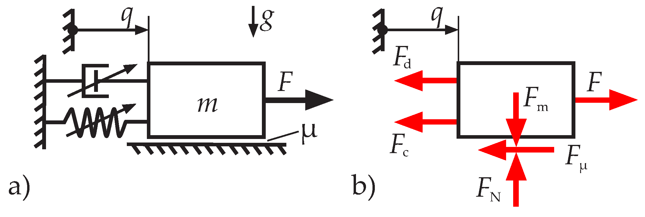
Figure 2.
Synthetic measurements (black) and results of the white-box model (gray).
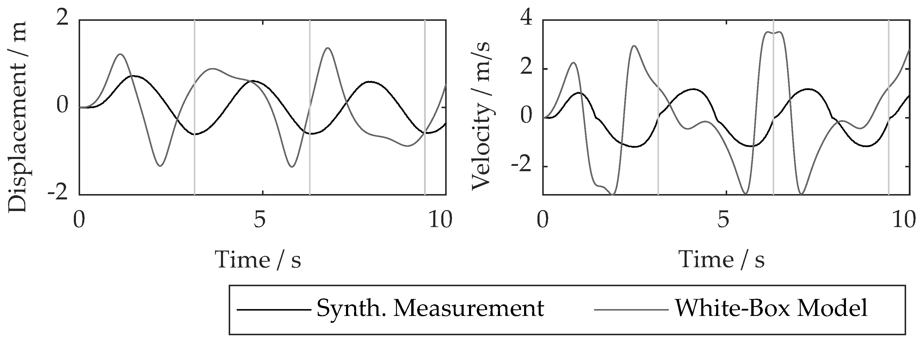
Figure 3.
Training (red) and test (black) data for the black-box model, as well as prediction results for the test data (blue).
Figure 3.
Training (red) and test (black) data for the black-box model, as well as prediction results for the test data (blue).
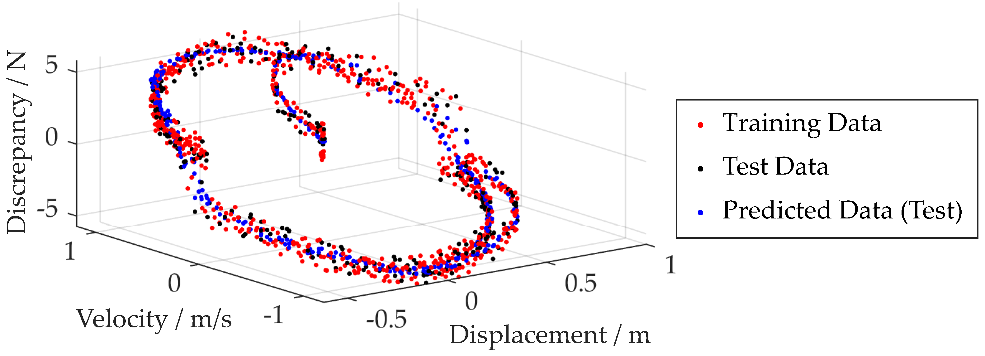
Figure 4.
a) Elements and b) model setup in MSC Adams and c) model setup in Simulink.
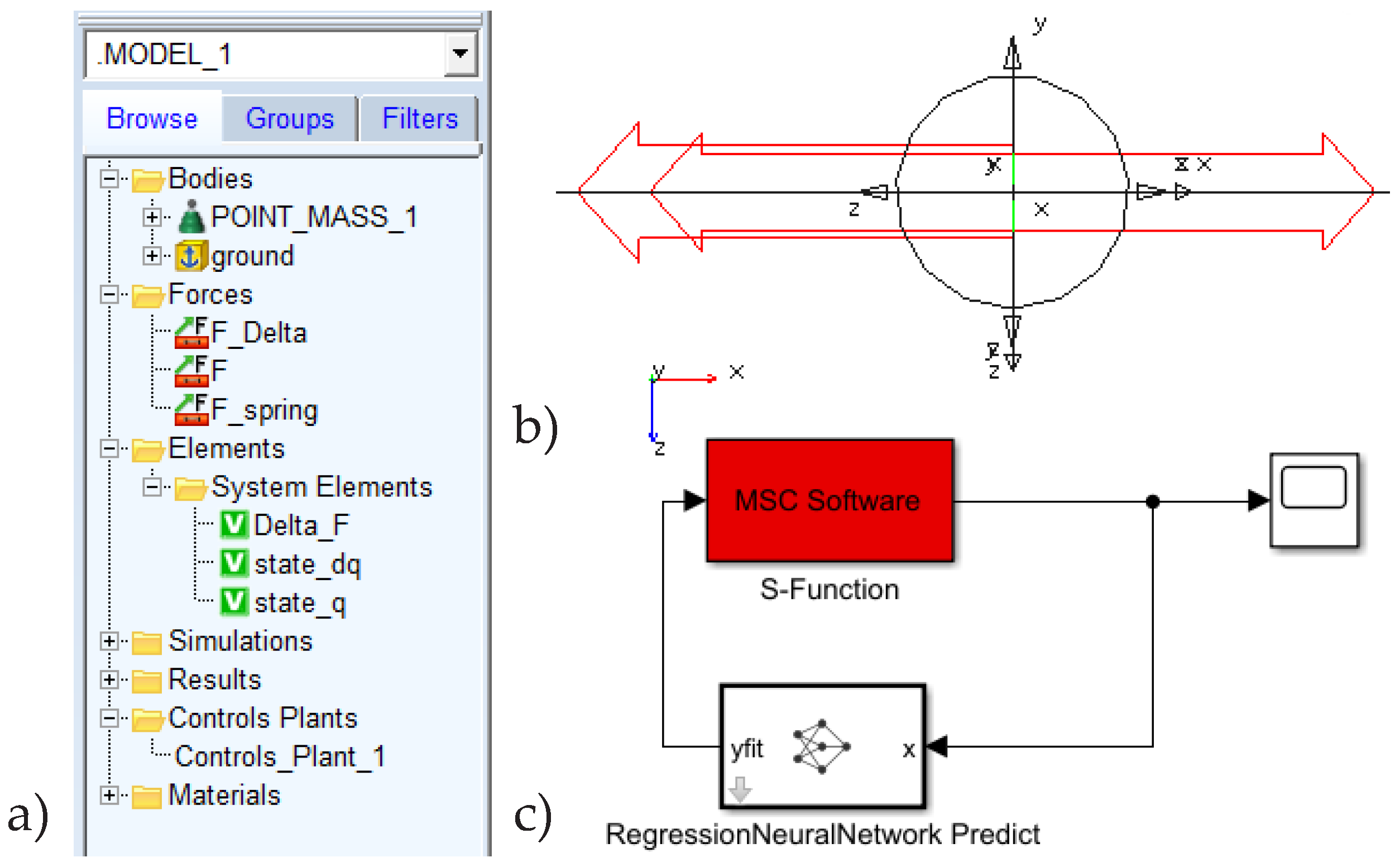
Figure 5.
a) Elements and b) model setup in Simpack and c) model setup in Simulink.
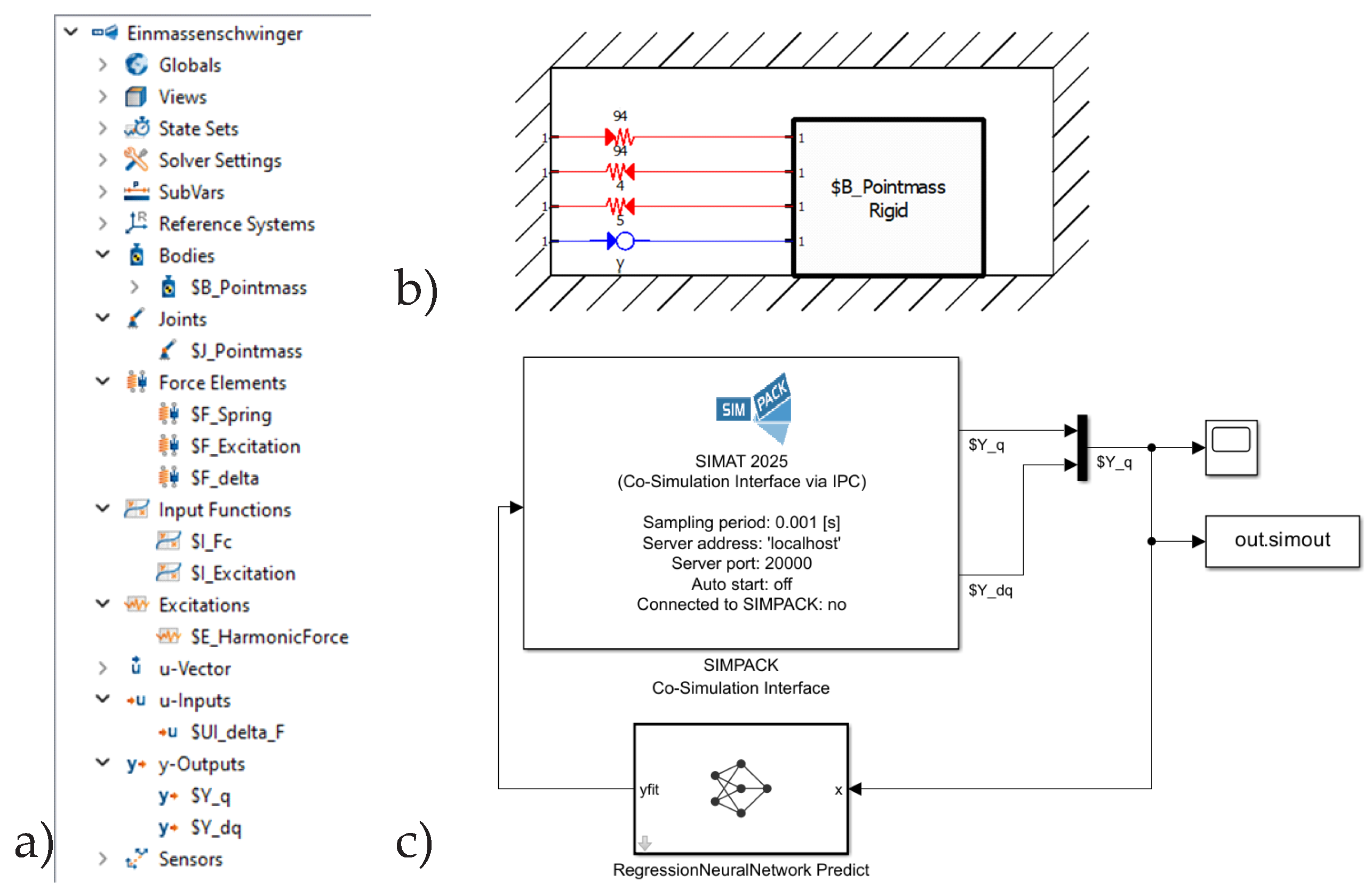
Figure 6.
Synthetic measurement and results of hybrid modeling.
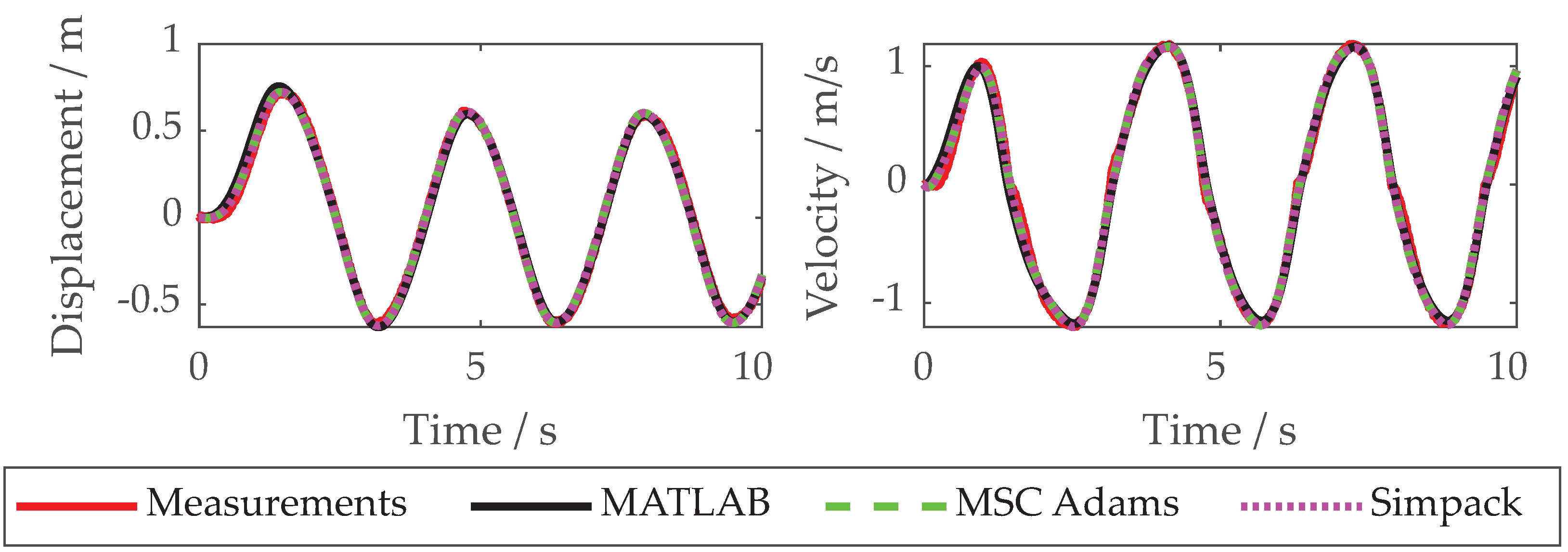

Table 1.
MAPE of the trained black-box models and RMSE for hybrid modeling in different software.
| Data-driven Model (NRMSE) |
train | test | train | test |
| MATLAB | MSC Adams | Simpack | ||
| Displacement (RMSE) | ||||
| Velocity (RMSE) | ||||
Disclaimer/Publisher’s Note: The statements, opinions and data contained in all publications are solely those of the individual author(s) and contributor(s) and not of MDPI and/or the editor(s). MDPI and/or the editor(s) disclaim responsibility for any injury to people or property resulting from any ideas, methods, instructions or products referred to in the content. |
© 2025 by the authors. Licensee MDPI, Basel, Switzerland. This article is an open access article distributed under the terms and conditions of the Creative Commons Attribution (CC BY) license (http://creativecommons.org/licenses/by/4.0/).
Copyright: This open access article is published under a Creative Commons CC BY 4.0 license, which permit the free download, distribution, and reuse, provided that the author and preprint are cited in any reuse.


