

Submitted:
03 March 2026
Posted:
04 March 2026
Read the latest preprint version here
Abstract
Motivated by Matsas et al. (2024), who demonstrated that time can serve as the fundamental unit for physical quantities, thereby obviating the need for traditional length–mass–time (LMT) dimensions, this study expands on some of the presented results. Using a Lorentz transformation (LT) matrix approach, we first validate the three-clock protocol, confirming distance derivation as a function of three proper clock times in a round-trip-like arrangement in Minkowski spacetime and additionally identifying moving clocks velocities without a distance measurement, which is already implicitly identified. The investigation was then extended to Tangherlini’s 4D spacetime framework (1958) to test the hypothesis that absolute velocity can be resolved through subluminal motion experiments. While initial three-clock scenarios resulted in systematic absolute velocity cancellation, a breakthrough was achieved by applying relativistic transverse Doppler effect logic. This approach successfully circumvents cancellation effects by identifying those electromagnetic waves in transit as becoming ‚anonymous‛ and owned by the Absolute Rest Frame (ARF), independent of source origin. We demonstrate that the ratio of transverse to longitudinal wave-vector components ky/kx provides a direct measure of the peculiar velocity relative to the Cosmic Microwave Background (CMB), fully reconciling with aberration angle methodologies utilised in Planck 2013 mission measurements. The findings reveal that both frameworks are mathematically equivalent representations of the same underlying reality, inevitably predicting absolute velocity despite historical objections. Consequently, a plausible absolute velocity methodology without instantaneous signals is proven possible, closing the "cancellation gap" via wave-vector geometry, and confirming the Tangherlini and special relativity theory (STR) frameworks.
Keywords:
absolute rest
; absolute velocity
; Tangherlini transformation
; postulate of relativity
; physical units
; relativistic transverse Doppler effect
; cosmic microwave background
; wave vector geometry
1. Introduction
In a 2024 study, Matsas et al. [1] introduced a compelling conceptual framework in which time serves as the sole fundamental unit for all physical quantities, thereby superseding the traditional length–mass–time (LMT) dimensional system. A particularly significant implication of this framework is the ability to measure spatial distance using only three inertial clocks. This is made possible by employing the Unruh protocol Bill Unruh, undisclosed private communication, according to [1]. This unusual measurement can be achieved via a round-trip configuration involving one stationary clock C3 and two relatively moving clocks C1 and C2, as illustrated in Figure 1. Although such a result is unattainable within a Galilean coordinate system, it becomes viable in Minkowski spacetime. This is because the reduction in degrees of freedom is caused by the implementation of Einstein’s light-speed isotropy postulate. The distance-measurement formula derived in [1] is based on the worldlines of three inertial clocks forming a triangle in a Minkowski diagram and is expressed as follows:
where is the C3 clock time at the stationary system origin, and and are the respective trip durations of moving clocks (C1 and C2) at unspecified velocities. This formula can be expanded to the following equivalent expression:
1.1. Experimental Protocol
In this study, we employed a motion protocol that differs slightly from the original arrangement in [1]; however it remains physically equivalent.
- Reference Frame: The stationary laboratory frame is designated as system B (base platform).
- Clock C1 Initiation: Clock C1 approaches from the negative -axis side at a constant, unknown velocity . When passing the origin, it is synchronised to .
- Base Synchronisation: The stationary clock C3 is simultaneously reset to at the moment of C1’s departure from the origin.
- Clock C2 Worldline: Clock C2 is launched from a distant point on the positive -axis at velocity on a reciprocal heading towards the origin. To ensure a continuous trajectory, a negligible -axis offset is assumed. Upon encountering C1 at an unknown position , C2 is synchronised to .
- Procedural Independence: Although this round-trip arrangement aligns with the triangular geometry in Minkowski spacetime used in [1], the individual legs of the trip can be executed sequentially in practice, as the recorded durations are independent of the specific epoch of initiation. The delay δ between the C1 arrivals and C2 arrival could be measured by an additional unsynchronised clock, similar to C3, located at . This would increase the accumulated total duration on clock C3. For derivation clarity, we assume that δ=0 to maintain consistency with the reference [1].
- Data Transmission C1: At the point of encounter with C2, clock C1 transmits its elapsed proper time to the origin of B to support future calculations, whereas C2 resets the time to 0.
- Data Transmission C2: Upon reaching the origin, clock C2 communicates the recorded duration to the base to support future calculations.
- Final Measurement: The stationary clock C3 records the total round-trip time , which represents the sum of the consecutive durations for clock C1 ( to reach the unknown distance and for clock C2 ( to reach the origin from .
Using this protocol, we confirm that the acquired data appear sufficient to resolve not only the unknown distance LB but also the previously undetermined velocities and . Additionally, an analysis of this scenario was performed in the 4D Tangherlini framework.
2. Methods
2.1. Background
Section 3 presents a validation of the distance formula in Equation (1) using the widely accepted LT matrix for relativistic kinematics. Although the validation of the distance was expected, the emergence of new velocity formulae in Equation (12) presented a distinct challenge. We recognise that the methodology must be adequate to the specific context in which the Tangherlini transformation (TT) is perceived. TT remains outside the mainstream; indeed, rejection is often declared a priori. Will [2] (pp 325,326), referencing the Mansouri-Sexl [3] generalisation of coordinates transformation, remarked that adopting the infinite signal speed required for absolute clock synchronisation is a “perverse choice.” Irrespective of conceptual difficulty infinite speed might cause, such terminology can stifle objective scientific discussion. However, Tangherlini methodically derived the transformation from Einstein field equations and was fully aware of the instantaneous signal problem, yet expressing hope for absolute velocity detection via subluminal signals or rotational motion. Unlike earlier attempts, such as Eagle [4], requiring electrically controlled vibrating quartz rods, or Mansouri-Sexl [3], whose derivation appears to stem from a misinterpretation of LT time coordinates [3] (p 301 eq. 3.4)—the methods adopted here seek to ground the discussion in objective, theoretical, and potentially measurable evidence.
2.2. The Adopted Approach
The following rules characterise our approach:
- We adopt the standard idealisations of imposed by the STR [5], including the Einsteinian definition of inertial systems where Newtonian mechanics holds, and the use of ideal rigid measuring rods abstraction within a Euclidean geometric framework.
- We assume that the TT applied to 4-vectors results in physically valid transformed quantities, unless a contradiction is proved, thereby granting the TT the same initial mathematical confidence as the LT.
- Confidence in the TT is further bolstered by the fact that, beyond Tangherlini’s general relativity (GR) approach, these transformations can be derived from the fundamental postulates presented in Appendix A.
- To maintain a clear focus on the correspondence (or lack thereof) between these theories, we intentionally exclude quantum theory or complex GR metrics. Following Descartes’ Rule of Analysis in Discourse on Method [6] p.35): we aim to “divide each difficulty into as many parts as required” to achieve clarity by not introducing associated important, but separate concerns. In commenting on light propagation we usually stay within the classical view proven useful in the original STR.
- Following Point 2, transformed physical quantities are deemed potentially measurable. The failure to determine absolute velocity excludes experimental confirmation; otherwise the theory must still be deemed theoretically sound and worthy of experimental effort.
- Similarly to the STR approach, in the Tangherlini framework we implicitly assume the same idealisations and simplifications of physical reality as presented in Point 1.
- Non linear system of equations frequently appear and they are solved using Maple™2019 algebra package. It is also used to verify transformations to reduce the chance of algebraic errors.
2.3. Notation Convention
In the following sections we introduce up to four coordinate systems: A representing the ARF, B for the base system and B1, B2 for clocks C1 and C2 respectively, which we recognise from the LT-based scenario. The notation used in this paper designates the last one or two symbols in the relevant variable’s suffix to determine in which frame the quantity is observed/measured, while one or two preceding characters may define the frame to which the quantity belongs or identify a specific feature; hence, denotes the velocity of system B as measured in A. Similarly, for the C2 clock’s system B2, we have , which is the velocity of system B2 in A. The symbol refers to a vector aligned with the -axis measured in system B1 and representing the length L. This allows for a unique distinction between similar quantities in different frames. The transformed vector symbols change the suffix sequence accordingly. Some symbols have additional superscript to relate them to time axes. The convention is that time in the reference rest system, is represented by simple variable and for relatively moving systems by , , as needed. In the transformation context, the same transformed quantity may be expressed as a function of the rest system time or that of the moving system time, therefore for example is the length vector in the moving system time coordinate, while the same in the rest frame coordinates is un-primed , both representing the same quantity.
3. Distance and Velocity Calculations in Minkowski Spacetime
The following derivations implicitly assume the idealisations and simplifications of the physical reality typical of the STR [5]. The preferred method for these derivations is linear algebra, utilising the Lorentz transformation (LT) matrix which is defined as follows:
We assume that a stationary inertial base system B, is represented by a 4D Cartesian coordinate system. Within this frame, we analyse the motion of two inertial point masses represented by clocks C1 and C2, moving along the -axis. The 4-vector represents an unknown, reference distance:
The transformation of the fixed in B to the local C1 coordinates using the LT matrix multiplied by yields the moving point approaching C1, which is at the origin of the inertial system designated as B1:
The transformed vector is initially expressed in terms of the base system time and must be converted to the local proper time of C1:
The converted vector in the local primed coordinates is obtained by substituting the expression for from Equation (6) and subsequent simplifications:
The time required for to come into contact with the C1 origin can be determined when , which is calculated from the following equation:
where is the proper time of clock C1.
C2 differs from C1 only in terms of the magnitude of the velocity and sign; hence, it can be deduced from Figure 1, then, by analogy,
In clock C3, the duration of the round trip is the sum of the successive durations on each segment as given by the following expression:
The minus sign in the denominator makes the C2 clock duration (proper time) positive.
Given that the clock times were measured, there are three equations and three unknowns: and , as follows:
The solution of the nonlinear system of equations (11) obtained by the Maple™ package with respect to and is as follows:
The expression for in (12) is valid only for the positive value. Although it appears algebraically distinct from the original Equation (1), it is equivalent to the expanded original form in Equation (2). The constant speed of light is absent in (2), because it was set to the dimensionless value of one in [1], in accordance with the Minkowski diagram convention.
Although we reject negative (unless it represents a coordinate on the negative side of ), we must decide which velocity variant to choose. In the scenario illustrated in Figure 1, it was found that, all the roots preceded by the plus sign represent the consistent solution of the system. Another feature of this system should be noted: The travel times of clocks C1 and C2 in B to , respectively can be calculated.
3.1. Conceptual Implications
The ability to measure using clocks alone is a noteworthy discovery by Unruh and Matsas et al. [1]; however, the capacity to obtain velocities without using presynchronised clocks is arguably more significant. Conventionally, velocity measurement requires two distant, synchronised clocks by definition: (with some exceptions, such as Doppler effect measurements or dual light-pulse round-trip measurements for uniform motion). Surprisingly, no explicit distance is necessary for the velocity expressions in Equation (12), because it is entirely factored into the temporal parameter arrangement. The three clocks, moving relative to one another, indicate their proper times without regard for any specific coordinate system; clocks possess no inherent knowledge of sensors or reference frames. Once we prove Equation (12), the result in Equation (13) is not unexpected. However, this simple and beautiful formula leads to the remarkable conclusion that three convention-independent invariant clock proper times can practically determine without any physical implementation of a coordinate system or pairwise synchronised clocks only, at most, by designating a distant point as without actually measuring it. The main thesis of one fundamental unit sufficient in physics postulated by Matsas et al. [1] is convincingly demonstrated. It may be premature to conclude that Equation (13) shows nature’s preference for a particular one-way velocity of light isotropy convention. Although duration was captured at locally in B1, all the equations leading to Equation (13) were derived using the STR framework. There are additional interesting consequences of Equation (13), which is discussed in Section 4.3.
These findings suggest that the three-clock-based measurement result is a natural consequence of the spacetime geometry. This prompted an investigation into the possible implications of the three-clock scenario within Tangherlini spacetime, introduced in the 1958 doctoral thesis at Stanford University [7]. Although the mathematical difference between the LT and the corresponding Tangherlini transformation (TT) matrices is subtle, the physical ramifications are vast. A scenario similar to that shown in Figure 1 can be applied by employing a hypothetical absolute ARF concept and three moving clock frames in relative motion.
4. Three Clocks in Tangherlini Spacetime
The transformation derived by Tangherlini provides an analytical relativistic framework similar to that in STR [5]. Originally named the “absolute Lorentz transformation” (ALT), the TT was derived from the Einstein field equations in the absence of gravitational sources. We found that the same transformation can be derived from first principles based on fundamental postulates, including the assumption of an ARF, as well as the experimentally established isotropy of the round-trip average speed of light and potentially controversial invariance of the instantaneous signal hypothesis (see Appendix A for the exact formulation of the postulates). No relativistic effects were assumed a priori; time dilation and length contraction emerged naturally.
Unlike the STR convention, where absolute velocity is outside the scope of measurement, we treat the ARF as a reference inertial system where is the absolute time variable; however, it is immeasurable. Thus far, according to the present consensus, absolute velocity suggestions appear fallacious, as once asserted by Eddington [8]. In contrast, Tangherlini attempted to reason about the possibility of detecting absolute motion based on the presented theory, but this was inconclusive at that time. First, he noted that if two distant clocks are not absolutely synchronised, it is not possible to calculate the one-way relative velocity of anything, because there is no way of correlating the time of arrival in terms of the time of departure [7] (p48). In Chapter 6 of [7] (p73–74), a suggestion is made that using subluminal signals, it would be possible to detect the absolute motion of the Earth. However, despite the focused, detailed analysis, no closed-form explicit solution or sufficient details of the measurement method demonstrating this possibility could be found. Additionally, in the final chapter of [7] (p101), Tangherlini concluded that in the examples presented in the doctoral thesis, absolute velocity always cancels out when measurements are performed “in the usual manner”. We assume that these methods do not depend on the prior absolute synchronisation of separated clocks, which seems to be impossible without instantaneous signals.
After determining that velocities can be measured with only three clocks, as shown in Equation (12), the question emerged as to whether this method was sufficiently ‘unusual’ to prove absolute velocity. The Unruh three-clock protocol [1] requires only three measurable proper times, and no two distant clocks appear to be synchronised, only by the coincidence of their positions in a predefined location to reset them to 0. We attempted the proof based on a methodology similar to that in Section 3, but with the TT matrix, which is represented as follows:
The infinity subscript in the TT matrix symbol emphasises the role of the instantaneous signal postulate. Matrix (14) differs from the LT matrix (3) because of the absence of the space-dependent time coordinate, which is now zero. Although the impossibility of absolute synchronisation with infinitely fast signals appears to be a fundamental obstacle, the significance of the TT framework would be profound if such obstacles could be circumvented.
4.1. Three-Clock Thought Experiment in Tangherlini 4D Spacetime
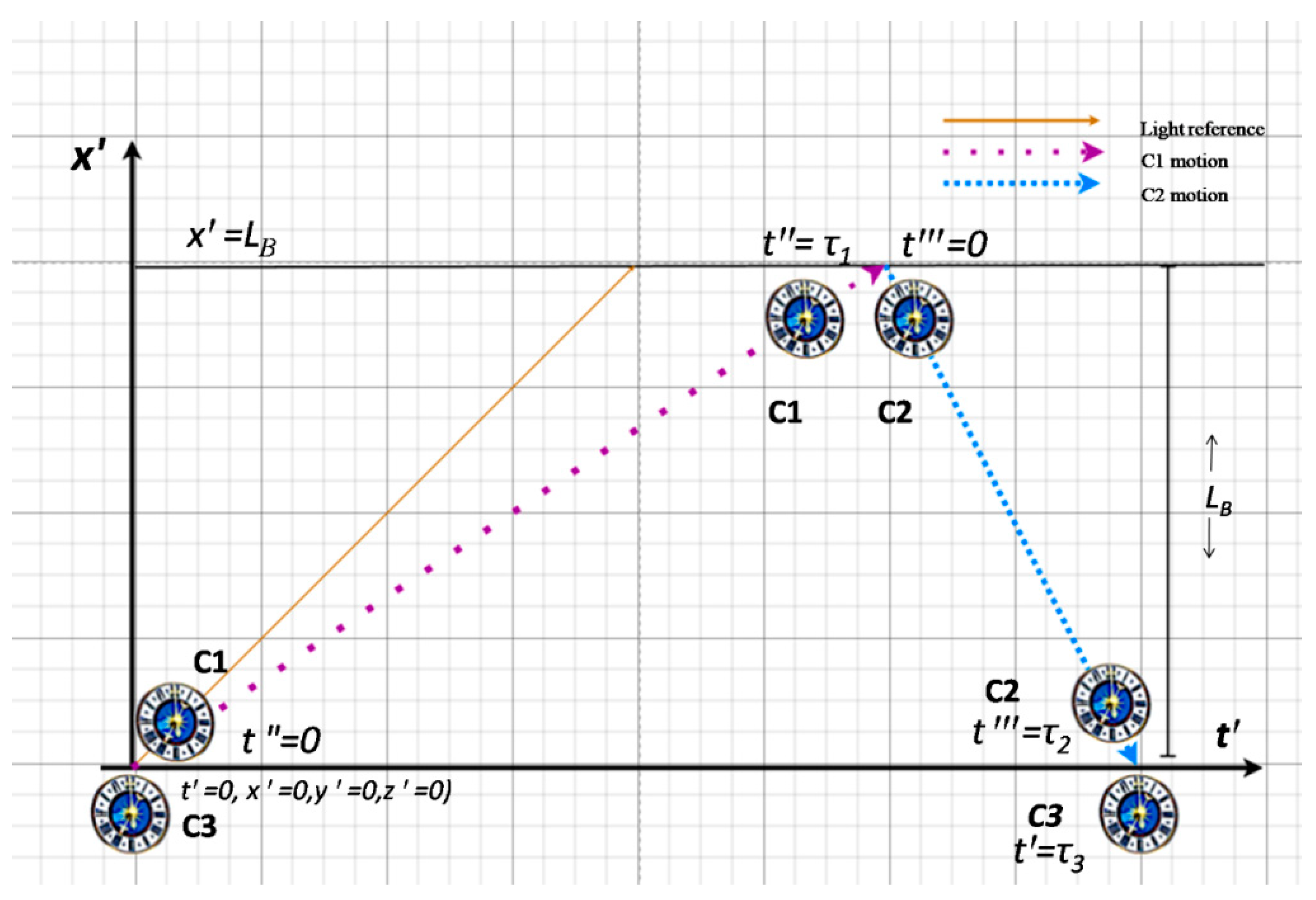
The graphical representation of the scenario differs slightly from that of the previous case in terms of axes symbols, as shown in Figure 2.
This shows the perspective of the base system denoted by B with the system clock C3, which is an inertial moving system with respect to the hypothetical ARF denoted by A, which thus far, according to the present consensus, cannot be identified. However, it is treated here as a special purpose inertial system with a time variable , wherein no measurement can be made because no reference points are known in empty space. The scenario is shown as if C2 starts instantaneously when C1 arrives, making it truly unrealistic but as explained on page 2. It can be programmed to arrive later and have a delay δ measured and factored in the equations accordingly. Therefore we proceed with the simplest case and assume fixed and zero delay .
In partial agreement with Poincaré’s [9] objections regarding the absolute space coordinate axes This idea came from Poincaré claiming that “absolute space is nonsense, and it is necessary for us to begin by referring space to a system of axes invariably bound to our body (which we must always suppose put backin the initial attitude).” With no features in space, the only way to bootstrap the derivation is to assume that at time t=0, some abstract coordinate system in A is momentarily aligned with the moving one and stays where it was as the distance increases. Absolute space then has no role other than being a passive container for inertial systems as far as this simple linear algebra model is concerned., we instead consider the absolute rest state to be a unique property of the subclass of inertial systems out of the class of all inertial systems rather than the state of the ‘void’. Our position disagrees with Newton’s concept of absolute space, which “remains always similar and immovable.” [10], but aligns with Einstein’s remark on the ether: “the idea of motion may not be applied to it” [11].
The inaccessibility of the featureless absolute space to measurement and the same with respect to any inertial absolute system A, can be overcome by using the inverse transformation (TT−1) from any inertial system where times and lengths are measurable and can be formally related to A, based on the presented model. Currently, absolute velocity remains hypothetical until its measurability is proved.
4.2. Derivation and Mathematical Reconciliation
In system B, we designate a fixed distant point as a 4-vector at which the worldline of C1 ends and that of C2 begins:
Instead of relative velocities as in the LT-based three-clock scenario, we look for absolute velocities with respect to the initially undefined absolute frame A. There is no obvious way to measure the relative velocity in Tangherlini spacetime; therefore, we need to introduce the base system’s absolute velocity vector in A with an unknown magnitude . For simplicity, as in the STR standard configuration, this vector is aligned with the virtual -axis of A and with the collinear x’-axis of B, as prescribed by the Tangherlini standard coordinate configuration (x-boost).
We can determine the vector equation of motion (EOM) of in A as by applying the inverse TT matrix .
The variable in B must be eliminated from the transformed vector so that the absolute time is consistently expressed in absolute coordinates.
can now be expressed in absolute time coordinates as follows:
The moving clock C1 is associated with the symbol B1, which represents its local coordinate system, and must be converted to this system, in which a fixed is considered to be a moving point towards the origin of B1. The absolute velocity of B1 in A is designated as . Therefore, it must be transformed using the transformation matrix .
The variable must be eliminated from the transformed vector so that can be consistently expressed in the coordinates.
After the substitution, can be expressed in B1 terms of the coordinate as follows:
The marker in the B1 frame appears to move towards the B1 origin. The time at which clock C1 coincides with the marker is when its coordinate is 0:
The trip duration of clock C1 is now determined. Because of the downwards worldline orientation, the duration of clock C2 follows the same formula (22), but with a different velocity symbol and with the sign inverted so that remains positive.
We have determined the durations on paths from the perspective of moving clocks C1 and C2; now, we need to find the relative velocities and of these clocks in B and the time of the round trip measured by clock C3. The vector EOM of C1 in A is given by the 4-vector :
Applying TT to yields the following:
After Equation (25) is converted to local time t’ of B, the relative EOM of C1 is expressed as follows:
Similarly, for B2:
The relative velocities and in Tangherlini spacetime are then obtained using the same formula except that is replaced :
The round-trip time registered by clock C3 is as follows:
We obtain the system of the following three nonlinear equations from Equations (22), (23) and (29):
From this system, we cannot calculate because we have three unknown velocities and therefore four unknowns, with only three equations. We cannot rely on the method described in Section 2 because it is not yet practically feasible. However, this is not an obstacle because is a free parameter that can be measured by traditional methods, particularly using the return time of the light signal on the round trip: .
The system solution was attempted using Maple™ 2019. Unfortunately, despite the unusual nature of the three-clock method, which does not explicitly rely on distant clock synchronisation, no solution was found because of the usual absolute velocity cancellation.
In confirming and analysing the disappointing but widely expected null result, an important connection was found between the Minkowski and Tangherlini frameworks.
- Using proper times represented by Equations (30);
- Substituting them into the positive root of the equation for LB and to all velocity roots denoted as using Equations (12); and
- Assuming that and is a real positive number, the result of algebraic simplification is as follows:
This was as expected for . The absolute velocities did cancel each other; thus, remained invariant. However, no cancellation was observed for the STR relative velocities. One instance of the STR velocity can be the result of an unlimited number of combinations of . Measuring any of the velocities from to is insufficient to solve for because of one extra degree of freedom. At this point, all the classic predictions seem to confirm the postulate of relativity as formulated by Poincaré [12] ( on June 5, 1905), placing the inability to detect the absolute movement of the Earth as the foundation (see the discussion on page 18). Poincaré reported that his principle, which is consistent with the Lorentz transformation, was thoroughly reviewed and rederived with full mathematical rigour [12]. This finding made it pointless for him and most of his successors to look elsewhere. However, the peculiar relationships in Equations (31) and their potential significance have triggered further investigations.
4.3. Variable Speed of Light vs. Conventional Isotropy
The variable light velocities in the standard coordinate configuration in the Tangherlini framework are given by:
where and are the positive variable magnitudes of the velocity of light on the -axis in the positive and negative directions, respectively; hence, all relative velocities are functions of absolute velocities. First, we analyse the results in Equation (13). Using the proper times given in Equation (30) and substituting them into the first equation of Equation (13), we obtain the following:
where is the current time coordinate at the instant of x= in the propagation of C1 in B in the LT-based scenario. One proper time corresponds to an unlimited number of pairs . The Lorentz coordinates with Tangherlini coordinates can be related knowing that their -axes are perfectly aligned thus x in Lorentz coordinates of B are the same as x’ in Tangherlini coordinates: . The common axes can serve as a bridge between the two theories.
In the Tangherlini framework perspective is the relative velocity of B1 in B given by the first Equation (28); therefore the variable distance travelled is:
where is the time coordinate in the Tangherlini framework at the instance of the distance . Both models have different coordinate labels because non-primed variables belong to the reference rest frames, which differ in both cases. For the motion from the STR perspective, the same motion is described as which according to Equation (31) expands to
where is the time coordinate in the STR framework. This leads to the following system which can be solved for and :
One of the two solutions including is of interest, from which the relationship between and can be found:
This allows bidirectional conversions between the Tangherlini and STR frameworks because the -axes are identical when they statically coincide in B. In four dimensions the conversion scheme between the Tangherlni and STR systems is: { }. This also indicates the irreducible degree of freedom because elimination from the scope. This degree of freedom is the main reason for all the cancellations. It was previously believed that removing this freedom could occur only by implementing the nonexistent instantaneous signal synchronisation. Fortunately, this is not the only option. An attempt to demonstate this, follows in the next section.
4.4. Closing the Cancellation Gap
Our attention has shifted towards identifying a missing equation that would allow for the recovery of the absolute velocity . The term ‘cancellation gap’ refers to the historical period when absolute velocity was categorically denied based on inevitable cancellations of assumed absolute velocity in many theoretical models, which denial continues until now. Thus far, our derivation of the TT has assumed an empty, featureless, and passive space, focusing on the relative kinematics between a hypothetical privileged inertial system and any other selected inertial systems. The relativistic TT was derived from the empirical law of isotropy of the average round-trip speed of light without assuming a specific physical cause for this behaviour. However, it is logical to conclude that this behaviour is not caused by inertial systems themselves. This raises a critical question: is there an overlooked property of light that could resolve the absolute velocity?
The most vital observation is that while light is emitted and absorbed by atoms to facilitate measurement, its orderly, causal propagation from a point on one inertial system to another point on the same or another system is related to a property of the vacuum and the nature of electromagnetic (EM) field itself. Once emitted, a beam of light exists independently of any inertial system, propagating as a coherent standalone entity—much like a ‘rigid rod’ of fixed length. Considering light from a distant star that may no longer exist, it travels through the void and interacts with any inertial system it encounters. At the moment of interaction, the original source is irrelevant; only the freely propagating beam matters. While a stationary observer in the ARF would measure an intrinsic frequency, a moving observer in system B would measure a changed frequency. This invites us to look beyond the average round-trip speed of light and examine the Doppler effect as an additional fundamental property. We consider a monochromatic EM wave, also referred to as radiation, propagating along the -axis from the positive side towards a detector and clock C3 at the origin of the base system B.
Let be the wave 4-vector of the outgoing wave from A in free space towards an observer described in the ARF as
The outgoing wave becomes an incoming wave in base system B. TT is applied to convert this vector to B as follows:
where .
The explicit presence of in the two components of the wave vector in Equation (39) suggests a mechanism for determining the absolute velocity, provided that the angular frequency and wave number can be accurately measured. However, a critical interpretive challenge arises: the temporal component of the transformed wave 4-vector in frame B cannot be regarded as the valid Doppler frequency.
Although Equation (39) shows the absolute frequency scaled by —a result that initially appears to be the ‘preferred frame’ asymmetry sought in this study—this derived frequency contradicts established analyses of absolute transformations. For instance, Sfarti [13] utilised the algebraic form of the TT to demonstrate that the resulting Doppler shift is identical to that of the STR. Other authors, such as Drągowski and Włodarczyk [14], confirmed this equivalence using an absolute transformation (following the Rembieliński framework).
This convergence is expected, given that TT is consistent with Einstein field equations; consequently, the choice of synchronisation convention should not alter the predicted physical observables. It is therefore necessary to clarify the mathematical discrepancy in the wave 4-vector transformation that suggests otherwise, specifically by examining how the induced longitudinal projection affects the temporal component with the expected relativistic shift.
To explain the mechanism underlying the LT result, a generic format of the wave 4-vector in the source S space is utilised.
LT is applied from a moving source S perspective to make predictions in B:
where is the LT matrix, is the velocity of base system B receding from the initial coincidence point with the radiation source system S and is the angular frequency in the source.
The reason for this difference is now clear. The temporal component is intertwined with the spatial component, unlike when using TT. Absolute time scaling by TT cannot reflect the frequency change because of the interaction with sensors, which are tied to the spatial coordinates of B. In practical terms, the TT effect yields an ideal local frequency that changes because of time dilation. This cannot be measured without the moving B-attached sensor physical interaction, which would change the frequency to the default value predicted by the STR. However, this is not the end of the problem. A more interesting result can be obtained by analysing the transverse Doppler effect.
Initially, we assume that “transverse” is relative to the observer in B, which is moving along the local axis. Therefore, the wave 4-vector must be appropriately “tilted” to propagate along the moving axis. Starting with the LT we obtain:
where is a function of velocity In the Planck 2013 space mission report [15], the referenced article by Challinor and van Leeuwen [16] explain the theoretical foundation of the transformation of the received radiation from the Cosmic Microwave Background (CMB), and provides a formula for the frequency in the CMB which was adapted to our notation as follows:
where is the photon propagation direction unit vector and is a spatial vector of magnitude . In the direction aligned with -axis in B, the formula changes to , and is the same as in the equation to obtained by comparing temporal elements in Equation (44). Our approach transforms motion from the CMB frame to B frame, whereas in [16] the CMB motion in the observer-centric system is preferred. Both approaches are equivalent as demonstrated in Equation (42).
Next, we consider the case in which the source emits radiation that is perpendicularly to the and axes.
A nonzero longitudinal wave number component emerges, which is absent in the source system emitting radiation, perpendicular to the and axes. Additionally, the transverse component exposes an unchanged stationary frequency in (if measurable). These are well-known facts.
In a standard scenario, the velocity of the system B can be measured using two consecutive round-trip experiments, and then is calculated after measuring and then substituting the experimental velocity value into the temporal element expression in Equation (44) to obtain . Subsequently, the theory can be tested by receiving information from the source to determine what the frequency was, then to verify whether it matches. However, what can be done if the source relative velocity is unknown because it is no longer present, and is also unknown because there is no one to measure it? The solution is in the ratio of R= .
We can now find the unknown velocity .
where is the aberration angle in the moving system B.
Using trigonometric identities we obtained /c, which is the same as the Einstein’s aberration formula in [5] (p56). These are frequency-independent expressions and the aberration angle can be measurable, as for example in the Planck 2013 mission [15].
The critical question remains: among infinitely many possible inertial systems, which one is responsible for this random wave? The source may no longer exist. We conclude that to maintain the propagation and frequency the only possible system remaining must be consistent with the ARF, wherein radiation always propagates even in the absence of particles. Relative spaces of inertial systems are abstractions and can only be involved through interactions such as measurements or by the presence of media affecting the speed of light. We acknowledge that radiation originates from moving bodies; however, in transit, we assume that EM waves become anonymous and ‘owned’ by the ARF. The original radiation sources no longer matter because any unique observed frequency can result from an unlimited number of combinations of source speeds and local frequencies which appears as an unsolvable ambiguity. However, Equations (46) are not ambiguous in B.
Although this conflicts with standard STR narratives that dismiss absolute velocity, it is supported by evidence: the speeds of the solar system and Earth have already been measured against the CMB using aberration angles in the sea of anonymous waves. This can also be verified in the Tangherlini framework:
We conclude that and have the same form of expressions as for the LT case; therefore, and are the same velocities of B relative to the ARF or the source frame S because we chose both S and the absolute system A to perform transformations predicting the effects in B. They generally agree, with at least one exception. While the relative velocity of S in B for the LT case is by definition, , this is different in the TT case. To obtain of the ARF velocity in B ( we need to transform the origin vector of S into B resulting in:
The exception is due to the STR clock synchronization convention; therefore, velocities acceleration, and other derivatives like momentum will never agree in numerical values; however, the predicted physical effects will all be the same, as we have demonstrated. Because we did not need to synchronise distant clocks anywhere in the universe with instantaneous signals and still identified the absolute velocity, Tangherini theory is a correct, convention-free special relativity theory. Although being conventional, the STR is an equally correct theory, as demonstrated. However, it is superior for practical use because it is not feasible to absolutely synchronise distant clocks based on the known velocity of the Earth, which fluctuates constantly, including the solar-centric and polar axis relative rotation.
Although we presented a limited derivation in the standard configuration of coordinates with an -axis-aligned absolute velocity vector, three-dimensional generalisations exist within the STR and TT frameworks. Chang [17] presented such generalisation for TT.
The absolute velocity derivation presented above, does not immediately necessitate novel experimental methods to detect it because this aspect has already been addressed in CMB research [15]. However, another method cannot be ruled out. The presented findings close the over-120-year gap in understanding the fundamental nature of Minkowski spacetime and naturally reconcile the concept of the CMB relative velocity with the current STR framework by making the “peculiar velocity” (Ellis and Baldwin [18]) compatible with the absolute one, owing to the concept of anonymous radiation introduced on page 17.
5. Discussion and Conclusions
5.1. Historical Perspective of the Absolute Velocity Problem
Given the contentious nature of the concept of absolute velocity, it is beneficial to consider its historical context to comprehend why it remained largely unexamined for an extended period.
The investigation of relative motion began to gain significant momentum around 1887 after the Michelson–Morley ‘null’ experiments [19], which demonstrated the constancy of the round-trip average speed of light, indicating in their opinion the lack of motion of the Earth in the supposed ether, contrary to well-known orbital and rotational motions. After their experiments, Michelson and Morley [19] stated that any relative motion between the Earth and the ether must be very small; however, we know that this is not the case.
Assuming one way velocity isotropy and the invariance of physical laws in all inertial frames, Einstein [20] rederived Lorentz transformation published in 1905, translated in [5] and special relativity was born.
Shortly before that, Poincaré [12] formulated one of the earlier versions (June 5, 1905) of the postulate of relativity which can be translated as follows:
It seems that this impossibility of experimentally demonstrating the absolute movement of the Earth is a general law of Nature; we are naturally inclined to admit this law, which we will call the Postulate of Relativity, and to admit it without restriction. Whether this postulate, which has so far been in agreement with experience, should be confirmed or refuted later by more precise experiments, it is in any case interesting to see what the consequences may be. Translation from [12] by Google Translate.
Unlike in Einstein’s systematic derivation approach, this formulation seems to assume the absence of absolute movement of the Earth a priori, without mentioning the problems related to one-way velocity measurement. The uncertainty expressed in the last sentence of the quote may explain the long-standing desire to detect the ether and the absolute motion relative to it. It also supports the idea of potential falsification. Poincaré referred to the electromagnetic radiation as vibrations of the ether until the end of his life; for example, in Last Essays [21]. The falsification option is presented in this study by deriving the velocity of an arbitrary system relative to an anonymous radiation source system S in Equation (46). The “impossibility of experimentally demonstrating the absolute movement of the Earth” as a law of nature is incorrect. However, it does not invalidate the principle of relativity in the vast majority of physical scenarios in the scope of STR.
The concept of absolute velocity and the variable one-way velocity of light have been rendered obsolete in contemporary physics. Nevertheless, certain researchers have persisted in exploring methodologies to circumvent the challenges associated with instantaneous synchronisation. Notable examples of such efforts are documented for example in the works of Mansouri and Sexl [22], Selleri [23,24], Tangherlini [25], Greaves [26], Spavieri, Gillies and Haug [27]. The emphasis is frequently on rotating frames and the empirically validated Sagnac effect.
5.2. The Significance of the Instantaneous Signal
The detectability of absolute motion is intricately linked to the concept of instantaneous signals, which have consistently been subjects of debate. An instantaneous signal is something that our intuitive understanding of time demands; however, this notion is generally deemed unscientific. There appears to be a consensus that simultaneity is inherently relative, and intuitive instantaneous perception is a mistaken generalisation, as noted by Canales [28]. Einstein [29] described this mistake as stemming from the failure to differentiate between what is simultaneously observed and what is simultaneously occurring. Nonetheless, he made a noteworthy observation during a discussion in 1911 [30] regarding the concept of a signal propagating infinitely fast, which would allow us to define time. This stands somewhat in contrast to the notion of time as defined in his 1905 paper [20] and [5] (in English).
The instantaneous temporal relation between distant events is typically understood as ‘now.’ This concept was officially dismissed by Eddington [8], who asserted that there was no absolute ‘Now,’ but rather a multitude of relative ‘nows’ unique to each observer. However, this concept proved difficult to relinquish for some physicists. According to Jammer [31] quoting Rudolf Carnap, the problem of ‘now’ was a significant concern for Einstein. Without delving into the full complexity of this issue, it is noted that the instantaneous temporal relation was a source of uncertainty for other physicists, such as Bell [32]. He posited the existence of a mechanism by which the setting of a measuring device influences the reading on another instrument at any distance, necessitating an instantaneous signal, thereby implying that the underlying theory cannot be Lorentz invariant. Without making any judgment on whether Bell’s signal can indeed be instantaneous or merely superfast, we acknowledge that Lorentz invariance exists within the STR convention and does not exclude superluminal signals contrary to popular belief. This is because they are not excluded in the Tangherlni framework which has proven to be consistent with STR. Apparent backward-in-time-travelling signals are merely convention-related synchronisation artefacts, akin to the case of crossing time zones in fast jets travelling in the East-West direction when one may arrive earlier than departed.
The nature of an instantaneous signal is such that it appears as a limit of a set of superluminal signals with ever-increasing velocity, none of which has a maximum value. This peculiar ‘signal’ can also be intuitively dismissed. Even the intuition of a creative mind, allowing for the instantaneous perception of the entire universe at once, may struggle to conceptualize a signal moving from here to a distant galaxy or beyond instantaneously, let alone finding the immediately reflected signal returning to the source at the exact moment of emission (but not earlier). Such an instantaneous signal appears to contravene causality based on simple local common-sense reasoning. At the time of emission, one might expect the signal to be delivered where it is not present. In considering the concept of transmission, one must address the paradox of its existence and return from a state of non-existence at the same moment because it is already coexisting at emission time. Typically, a signal can be characterised as a brief EM pulse or a minute particle, such as a photon or a tachyon. The notion of an infinite velocity implies that the signal does not traverse space; rather, it is omnipresent and absent at the same moment of emission. However, mathematics offers a more accommodating framework than mere imagination. The concept of instantaneous signal velocity, represented by an unbounded numerical series without a definitive maximum, mitigates concerns regarding intuitive non-causality, as such a scenario appears physically impossible. The sequence of emission and return events remains intact, irrespective of the brevity of the interval between them. This unattainable limit demarcates the boundary of causality and coexistence, with the latter not necessarily being experimentally accessible by signals. This perspective on the instantaneous signal, however, is inherently open to scientific scrutiny. The absence of observable instantaneous signals in nature has historically hindered philosophers and scientists from synchronising time across distant locations. The primary obstacle is the issue of circularity, in which two clocks at separate locations must display the same time simultaneously, with ‘simultaneously’ defined as events occurring at the same time. Einstein addressed this dilemma by postulating a constant one-way velocity of light and synchronise distant clocks accordingly, thus cutting the Gordian knot.
We have successfully demonstrated that no instantaneous signal is necessary to determine the absolute velocity in the Tangherlini and STR frameworks, both theories consistently represent the same reality, comparable to two faces of the same coin or two maps of the Earth in different projections.
5.3. Peculiar Velocity vs. Absolute.
The peculiar velocity term is usually defined as the deviation of galaxies’ velocity from the Hubble flow [33], but it is also commonly used as the velocity relative to the CMB. For example Ellis and Baldwin [18] stated that “the standard interpretation of the dipole anisotropy in the microwave background radiation as being due to our peculiar velocity in a homogeneous isotropic universe” other interpretations regard this velocity as relative to a locally defined common rest frame. It is uncommon to refer to the peculiar velocity as absolute velocity because the STR does not define such a category. Otherwise, it might as well be true the CMB in our local region may not be the same elsewhere, even though there is no evidence of that. In the presented approach, the rest frame emerged as an anonymous, unavoidable and unique reference frame representing an inertial system that justifies the Doppler effect when a radiation source and frequency cannot be identified. This emerged from purely kinematical considerations using the STR framework and the properties of the wave vector, resulting in Equation (48). This is in agreement with Einstein’s [5] (p56) derivation of the Doppler effect and the aberration angle. Subsequently, this result was also consistent with the Tangherlini framework where the ARF is a fundamental postulate. Linear algebra underlying our approach to the STR does not know the boundary of the universe; therefore the ARF theoretically extends to infinity and such ARF generalisation could be premature. It is more appropriate to say that the emergent ARF extends to the area wherever light propagates. We may call peculiar velocity absolute within these bounds. The STR does not support absolute velocity and the ARF; however, if the latter is found, it will not differ from any other inertial system, as demonstrated by CMB methods [15,16], and our results. These findings were unexpected, despite the crucial role played by the LT in determining the solar system velocity with respect to the CMB. The unusual nature of our findings is reflected by the long-standing view of late Jose G. Vargas [34]: “there is more to structure in special relativity than meets the eye.”
5.4. Results
The initial goal of this research was to verify whether an unusual method based on the Unruh protocol presented by Matsas et al. [1] could provide an opportunity to detect the ubiquitous absolute velocity because this method appears independent of the three distant clocks synchronisation in the inertial frame of interest B. This was an attempt to verify Tangherlini’s suggestions that the absolute motion of the Earth could be detected using subluminal signals, as mentioned on page 7. In the process, several interesting results were obtained.
- The three-clock scenario based on the Unruh protocol described by Matsas et al. [1] in Minkowski spacetime was implemented as an algebraic, STR-based model, leading to the system of equations (11). The system had solutions (12) consisting of eight roots, half of which were of the opposite sign to their counterparts. The original distance formula from [1] is fully reproduced by the first solution in Equations (12). Two previously unpublished relative velocity expressions for moving clocks not presented in [1] emerged.
- Owing to established dependencies, an important connection between the Tangherlini and STR frameworks has been revealed, indicating the complementarity of the former rather than being antagonistic or irrelevant. We derived the coordinate conversion equations between the standard STR and Tangherlini coordinates as: , resulting from Equations (36) and (37). This shows that the two theories are closely related and free of contradiction through a shared foundation, rather than juxtaposition without true correspondence. Only practical usefulness keeps them apart.
- Our hypothesis of the possible detection of the absolute velocity using subluminal signals based on the ‘unusual’ model represented by Equations (30) was not confirmed, as the absolute velocities still cancelled out “in the usual manner” [7] (p101), even though no explicit distant clock synchronisation was needed in the stationary system in the Tangherlini framework.
- Our research continued despite the first null result and succeeded, although not outside uniformly translating systems as suggested by Tangherlini [7] (p105). The missing extra equation was found from the transverse Doppler effect, which is measurable in the moving system, as shown on Page 15. This was first achieved using the STR approach. We presented possibility of determining the velocity of the base system B () by deriving the aberration angle expression in Equation (46) and similar for the absolute velocity in Tangherlini framework, both indistinguishable.where is the transverse Doppler effect-induced aberration angle and is the relative velocity of the moving base system B in an undisclosed radiating source system S and is the absolute velocity. Both A and S have the common feature of the isotropy of the round-trip average speed of light. The wave vector has two nonzero components sufficient to derive the expressions above, without knowing anything about the undisclosed system’s emitter velocity or the frequency. This approach has not been explored earlier because stationary and moving system examples in the literature always explored known two or more inertial systems, where physical quantities can be measured. The present example invokes an anonymous system from which only the incoming wave is measured. This is somewhat related to the CMB radiation, where no microwave can be linked to a particular emitter initial state.
- The Tagherlini framework and the corresponding STR allowed the detection of what we have defined as the absolute velocity in the assumed ARF. In the context of the existing CMB it does not appear peculiar anymore. Whether referring to it as ‘the absolute’ in the context of the universe governed by theories other than special relativity, it requires further scrutiny. The presented approach calls for a public discussion because of the long-standing controversy. Finding a Lorentz transformation capable of reconciling this controversy was entirely unexpected.
5.5. Conclusions
- The three-clock scenario presented in Section 4.2 was expected to help circumvent absolute velocity cancellation because the clocks were not synchronized using Einstein’s convention. This hypothesis was proven false; however, it revealed that the STR and Tangherlini frameworks are equivalent representations of the same reality. One three-clock scenario in the STR framework maps to an unlimited number of absolute velocity combinations in the Tangherlini framework, proving that their relationship is consistent and not accidental.
- Despite this general consensus, the absolute velocity can be detected by measuring the transverse Doppler effect modelled within the STR framework and confirmed to match the Tangherlini framework solution. This measurement is physically tied to the aberration angle () extraction utilized in CMB missions (e.g., Planck 2013 [15]). The difference is in the choice of the stationary system: while CMB analysis typically utilises a moving observer-centric approach [16], the presented solution utilises an anonymous radiation source-based approach. Both approaches were found to be fully equivalent, and reconciliation with the STR framework is evident. The reconciling equations derived from the ratio are in the STR framework and Tangherllini framework respectively.
- Poincaré’s postulate of relativity, based on the impossibility of detecting absolute motion, has survived for over 120 years because one equation—present but unsuspected to be the key in Einstein’s 1905 paper [5,20] — was missing to close the absolute velocity cancellation gap. Textbooks and other publications focusing on two-frame, well defined scenarios have overlooked cases in which the radiation source is unknown, yet the wave vector holds sufficient geometric information regarding the wave relationship to a moving object in the ARF. Although absolute velocities have no influence on physical processes, the transverse Doppler effect in EM waves is a notable exception.
- We conclude that when in transit, EM waves become anonymous and “owned” by the ARF. Original radiation sources no longer matter because any emission may be stopped, and any unique observed frequency may result from an unlimited number of combinations of source speeds and local emission frequencies.
- The famous Andromeda paradox, as presented by Penrose [35] (p 260), is no longer valid because it relies on conventional “tilted” time axes for two observers that do not reflect absolute simultaneity.
- This study realigns physics with the reality of absolute velocity. No experimental result confirmed within STR is invalidated; however, narratives dismissing absolute motion must be reviewed. We hope that the results will spur further research to expand and unify knowledge [35].
Author Contributions
The author contributed to all aspects of the work.
Funding
This research received no funding.
Institutional Review Board Statement
Not applicable.
Informed Consent Statement
Not applicable.
Data Availability Statement
New data were generated from the mathematical model. Detailed Maple computation results may be available upon request.
Conflicts of Interest
The author declares no conflicts of interest.
Abbreviations:
The following abbreviations are used in this manuscript:
| ALT | Absolute Lorentz Transformation |
| ARF | Absolute Rest Frame |
| CMB | Cosmic Microwave Background |
| EOM | Equation of Motion |
| GR | General Relativity |
| LT | Lorentz Transformation |
| STR | Special Theory of Relativity |
| TT | Tangherlini Transformation |
Appendix A. On Absolute Rest, Velocity and Tangherlini Transformation
Tangherlini’s [7] derivation of the transformation referred to in this study was originally based on the Einstein field equations, resulting in transformation equations compatible in structure with the LT equations derived by Einstein, as presented in [5] (p48). The arrangement of the two relatively moving coordinate systems can be referred to as the standard configuration, where the relative velocity vector is aligned with the first spatial axis (usually x). The mathematical representations of the TT, the postulates leading to its derivation and resulting properties are collectively referred to as the TT framework.
With respect to the TT framework, the ARF must be postulated a priori to allow different derivation processes using a method other than that of Tangherlini. For example, Selleri [23] defines the ARF as the one in which the velocity of light is the same in any direction, without demanding that moving frames follow the same rule. The impossibility of absolute synchronisation with instantaneous signals—let alone without them— appears to be the fundamental obstacle to the use of TT on a larger scale. The TT framework appears to be the only sensible but impractical alternative to the STR framework. Both frameworks share the same foundation, namely, the empirical law of isotropy of the round-trip average speed of light discovered by Michelson and Morley [19].
The TT framework can be derived from the first principles of Newtonian kinematics without reference to inertial rotational motion or the forcing postulates of length contraction or time dilation, as in some previous approaches. However, the frequently analysed Sagnac effect appears to be a legitimate approach.
The necessary and sufficient set of postulates and constraints for completely defining the TT is as follows:
Postulate 1: There exists an absolute rest frame represented by an inertial system A, with three Cartesian coordinate axes that can be bound (aligned) to preexisting axes of an inertial system M at time t=0 and t’=0. In that system, the one-way velocity of light is constant and equal to c in all directions, and there is only one system A (together with all its possible translations and rotations, all being at rest with it).
Postulate 2: The round-trip average speed of light in any inertial system is a constant, whose value c= 299792458 m/s, and is independent of the relative direction and velocity of those systems.
Postulate 3: An instantaneous signal being represented as the limit of all signals moving in the same direction with ever increasing velocity , observed in the absolute inertial system A as , is invariant in all inertial frames such that when observed in an inertial moving system M of the absolute velocity vMA, it is , where .
Constraint 1: The spatial origin of system M moving in the system A coordinates transforms to the origin point in M at rest with itself as M(0,0,0) at every instance of time t’.
Constraint 2: The determinant of the linear coordinate transformation matrix is equal to +1, as in the case of the LT and Galilean transformation matrices.
The TT matrix meeting the postulates and constraints can be derived and is shown in Equation (14). Including the full derivation process in this paper would exceed a sensible publication word count limit.
References
- Matsas George, E. A. The number of fundamental constants from a spacetime based perspective. Scientific Reports 2024, 14, 22594. [Google Scholar] [CrossRef]
- Will M. C., Theory and Experiment in Gravitational Physics; Cambridge University Press: Cambridge, 1993.
- Mannnsouri, R.; Sexl, R.U. A Test Theory of Special Relativity: I. Simultaneity and Clock Synchronization. General Relativity and Gravitation 1977, vol. 8(no. 7), 497–513. [Google Scholar] [CrossRef]
- Eagle, A. A criticism of the special theory of relativity. Lond. Edinb. Dubl. Phil. Mag. & J. Sci. vol. 26, 410–414, 1938. [CrossRef]
- Einstein, A. “On the Electrodynamics of Moving Bodies,” in The Principle of Relativity; Dover Publications, Inc.: USA, 1923; p. 140. Available online: https://archive.org/details/principleofrelat0000halo/page/n3/mode/2up.
- Descartes, R. Discourse On The Methodof Conducting One’s Reason Well and of Seeking the Truth in the Sciences; Press of Jan Maire: Leiden, 1637; Available online: https://dn710004.ca.archive.org/0/items/descartes-discourse-on-method-heffernan-archive/.
- Tangherlini, F.R. The Velocity of Light in Uniformly Moving Frame- PhD Disertation Stanford University1958. The Abraham Zelmanov Journal 2009, vol. 2, 44–110. [Google Scholar]
- Eddington, A.S. The Nature of the Physical World; Cambridge University Press: Cambridge, 1929; Available online: https://www.gutenberg.org/cache/epub/72963/pg72963-images.html.
- Poincaré, H. The Value of Science; Science Press: New York, 1907. [Google Scholar]
- Newton, I. The Mathematic Principles of Natural Philosophy; Daniel Adee: New York, 1848. [Google Scholar]
- Einstein, A. “Ether and the Theory of Relativity,” in Sidelights on Relativity; METHUEN & CO. LTD.: London, 1922; Volume ch. 1, p. 24. [Google Scholar]
- Poincaré, H. Sur la dynamique de l’électron. Rendiconti del Circolo Matematico di Palermo 1906, 21 vol. 21, 1906, 129–176. pp. 129–176. [Google Scholar] [CrossRef]
- Sfarti, A. Necessary Conditions for Equivalence with the Special Theory of Relativity. Lith. J.Phys. 2009, vol. 49(no. 4), 383–388. [Google Scholar] [CrossRef]
- Drągowski, M.; Włodarczyk, M. The Doppler Effect and the Anisotropy of the Speed of Light. Found Phys. 2020, vol. 50, 429–440. [Google Scholar] [CrossRef]
- Aghanim, N. Planck 2013 results. XXVII. Doppler boosting of the CMB:Eppur si muove. Astronmy and Astrophysics 2014, vol. 571(no. A27), 1–11. [Google Scholar] [CrossRef]
- Challinor, A.; van Leeuwen, F. Peculiar velocity effects in high-resolution microwave background experiments. Phys. Rev.D 2002, vol. 65(no. 10), 103001. [Google Scholar] [CrossRef]
- Chang, T. Maxwell’s Equations In Anisotropic Space. Phys. Lett. 1979, vol. 70A(no. 1), 1–2. [Google Scholar] [CrossRef]
- Ellis, G. F. R.; Baldwin, J. E. On the expected anisotropy of radio source counts. 1984, vol. 206(no. 2), 377–381. [Google Scholar] [CrossRef]
- Michelson, A. A.; Morley, E. W. On the relative motion of the earth and the luminiferous ether. Am. J. Sci. vol. 34(no. 203), 333–345, 1887. [CrossRef]
- Einstein, A. Zur Elektrodynamik bewegter Körper. Annalen der Physik, Band 17 1905, vol. 17, 1905. Available online: https://dn790008.ca.archive.org/0/items/zurelektrodynami00aein/zurelektrodynami00aein.pdf. [CrossRef]
- Poincaré, H. Mathematics and Science:Last Essays; Dover Publications, Inc.: New York, 1963; Available online: https://henripoincarepapers.univ-nantes.fr/chp/hp-pdf/hp1963ms.pdf.
- Mannnsouri, R.; Sexl, R.U. A Test Theory of Special Relativity: I. Simultaneity and Clock Synchronization. General Relativity and Gravitation 1977, vol. 8(no. 7), 497–513. [Google Scholar] [CrossRef]
- Selleri, F. “Noninvariant One-Way Speed Of Light And Locally Equivalent Reference Frames,” Found. Phys. Lett. 1997, vol. 10, 73–8. [Google Scholar] [CrossRef]
- Selleri, F. “Noninvariant One-Way Velocity of Light,” Found. Phys. 1996, vol. 26, 641–664. [Google Scholar] [CrossRef]
- Tangherlini, F. R. Galilean-Like Transformation Allowed by General Covariance and Consistent with Special Relativity. Journ. Mod. Phys. 2014, vol. 5, 230–243. [Google Scholar] [CrossRef]
- Greaves, E.D.; Ruiz-Camacho, J.; Rodrigues, A.M. A one-way speed of light experiment. American Journal Of Physics 2009, vol. 77(no. 10), 894–896. [Google Scholar] [CrossRef]
- Spavieri, G.; Gillies, E. G.; Haug, G.T. The Sagnac effect and the role of simultaneity in relativity theory. J. Mod. Opt. 2021, vol. 68(no. 4), 202–216. [Google Scholar] [CrossRef]
- Canales, J. Einstein, Bergson and the Experiment That Failed:Intellectual Cooperation at the League of Nations. MLN 2005, vol. 120(no. 5), 1168–1191. [Google Scholar] [CrossRef]
- Einstein, A. Physics and Reality. Journal of the Franklin Institute vol. 221(no. 3), 377–378, 1936. [CrossRef]
- Einstein, A. “”Discussion” Following Lecture Version of “Theory of Relativity”,” in The Collected Papers of Albert Einstein. In The Swiss Years Writings 1909-1911 (English translation supplement); Princeton University Press: Princeton, 1994; Volume 3, Available online: https://einsteinpapers.press.princeton.edu/vol3-doc/478.
- Jammer, M. Concepts of Simultaneity: From Antiquity to Einstein and Beyond; Johns Hopkins University Press: Baltimore, 2006. [Google Scholar]
- Bell, J. S. On the Einstein Podolsky Rosen paradox. Physics 1964, vol. 1, 195–200. Available online: https://journals.aps.org/ppf/pdf/10.1103/PhysicsPhysiqueFizika.1.195. [CrossRef]
- Springbob, C. M. The Galaxy 6Df Survey: peculiar velocity field and Cosmography. MNRAS 2014, vol. 446, 2677–2697. [Google Scholar] [CrossRef]
- Vargas, J. G. U(1) SU(2) from the tangent bundle. J. Phys.: Conference Series 474 2013, 1–17. [Google Scholar] [CrossRef]
- Penrose, R. The Emperor’s New Mind; Oxford Unversity Press: New York, 1999. [Google Scholar]
Figure 1.
The three-clock scenario (angles not to scale).
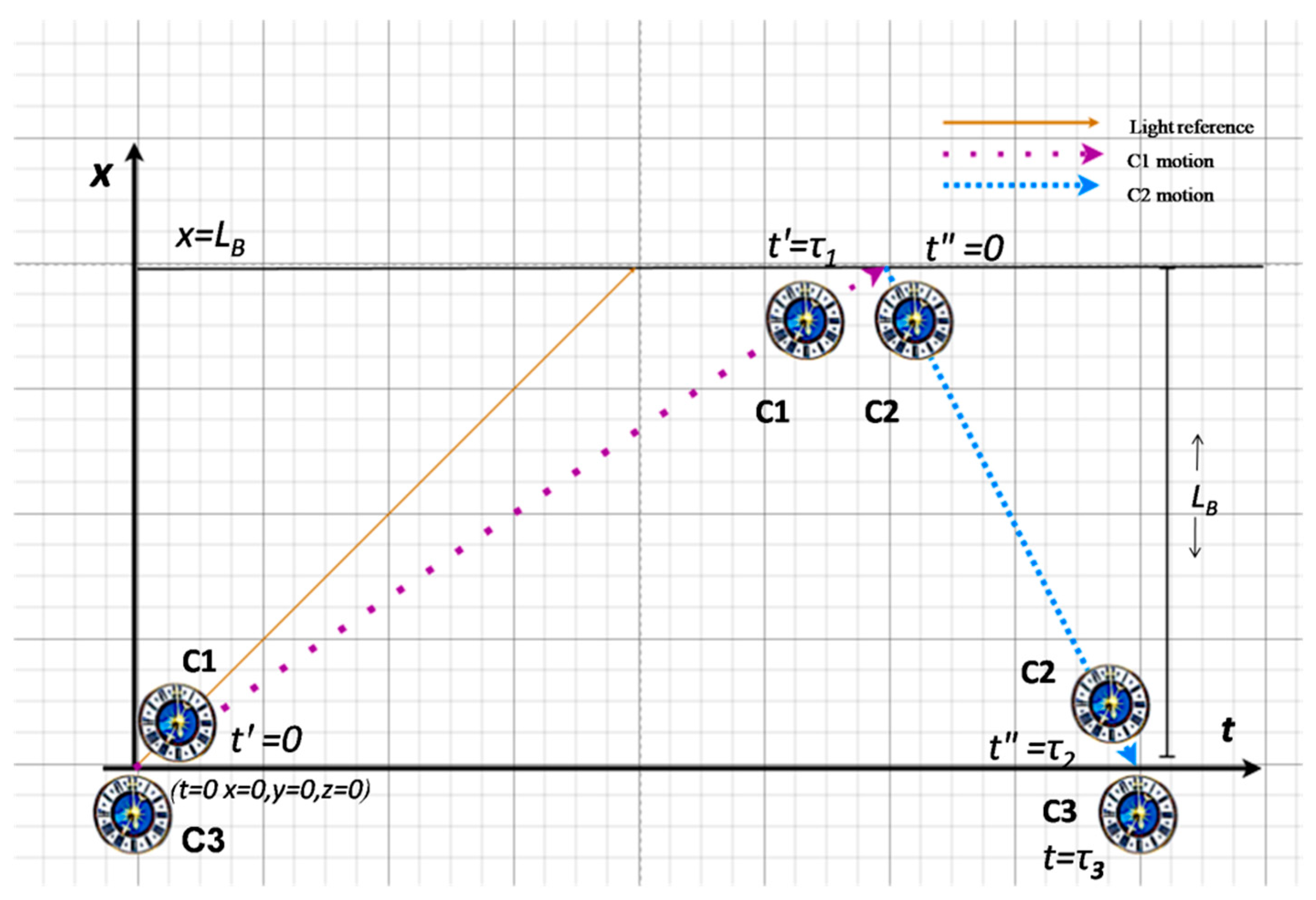
Figure 2.
Two-clock round-trip scenario in system B (angles not to scale).
Disclaimer/Publisher’s Note: The statements, opinions and data contained in all publications are solely those of the individual author(s) and contributor(s) and not of MDPI and/or the editor(s). MDPI and/or the editor(s) disclaim responsibility for any injury to people or property resulting from any ideas, methods, instructions or products referred to in the content. |
© 2026 by the author. Licensee MDPI, Basel, Switzerland. This article is an open access article distributed under the terms and conditions of the Creative Commons Attribution (CC BY) license (http://creativecommons.org/licenses/by/4.0/).
Copyright: This open access article is published under a Creative Commons CC BY 4.0 license, which permit the free download, distribution, and reuse, provided that the author and preprint are cited in any reuse.