
Submitted:
05 January 2026
Posted:
06 January 2026
You are already at the latest version
Abstract
To address the issues of detail loss and unstable segmentation quality in image segmentation, this paper proposes a muti-strategy improved dung beetle optimization algorithm and applied to muti-threshold image segmentation, thus, we have developed a Multi-strategy Improved Dung Beetle Optimizer Kapur entropy Multi-threshold Image segmentation Algorithm (MIDBO-KMIA). This algorithm enhanced global search capability and convergence stability, improved segmentation accuracy and algorithm robustness, and solved the problems of detail preservation and segmentation quality in complex scenarios. Firstly, Sobol sequences were adopted to initialize the population, enhancing its diversity. Secondly, a muti-stage perturbation update mechanism was introduced to prevent convergence to local optima and improved global exploration. Thirdly, the convergence precision was further improved by optimizing the hybrid dynamic switching mechanism and proposing dynamic mutation update and distance selection update strategies. Finally, the MIDBO algorithm was applied to Kapur entropy multi-threshold image segmentation, and experimental research was conducted using Peak Signal-to-Noise Ratio (PSNR), SIMilarity index (SSIM), and Feature SIMilarity index (FSIM) as evaluation metrics. The experimental results demonstrate that the performance of the multi-strategy improved dung beetle optimization Kapur entropy multi-threshold image segmentation algorithm is significantly better than other algorithms, which can more effectively solve the problems of detail preservation and segmentation quality in complex scenes, and enhance the ability to adapt to complex image scenes.
Keywords:
multi-strategy
; dung beetle optimization
; multi-threshold image segmentation
1. Introduction
Image segmentation technology is the main task of image analysis and recognition [1], which involves segmenting the target image into multiple regions with unique attributes and extracting regions of interest from them [2]. There are many methods for image segmentation, among which threshold-based segmentation methods can determine segmentation thresholds based on local or global information of the image, including single threshold segmentation and multi threshold segmentation. In practical life, the application of multi-threshold segmentation is more widespread [3].
The multi-threshold selection methods for images include maximum blur entropy [4], minimum cross entropy [5], and Tsallis entropy [6]. Since the one-dimensional threshold segmentation method employed the one-dimensional histogram of the image for calculation, the spatial information of the image has not been fully utilized. Therefore, some scholars have introduced neighborhood grayscale information of pixels and proposed entropy threshold segmentation methods based on two-dimensional histograms of images, such as two-dimensional arbitrary entropy threshold method [7]. and two-dimensional Tsallis entropy threshold method [8]. However, the existing multi-threshold segmentation methods have higher computational complexity, and as the number of thresholds increases, the computational cost required to find the optimal threshold also increases [9]. When processing large amounts of image data, the increase in computation complexity will be more pronounced.
The swarm intelligence optimization algorithm is mainly a metaheuristic algorithm that simulates the collective behavior of animals to achieve optimization. Due to its simple principles, easy implementation, and high optimization efficiency, it is widely used to solve optimization problems such as workshop scheduling, path optimization, and feature selection etc. So far, various swarm intelligence optimization algorithms, such as the Whale Optimization Algorithm (WOA) [10], the Artificial Bee Colony (ABC) [11], Grey Wolf Optimizer (GWO) [12], Snake Optimizer (SO) [13], Beetle Antennae Search(BAS) [14], Multi-Verse Optimizer (MVO) [15], and Flower Pollination Algorithm (FPA) [16], etc. have been applied to optimization problems in different fields. Therefore, many researchers try to combine intelligent algorithms with image segmentation methods, and optimize algorithms in different ways for different algorithms to improve the accuracy and speed of image segmentation.
Mahajan et al. [17] proposed a novel technique for multi-level threshold combined Fuzzy Entropy Type II (FE-TII) with metaheuristics. Zhao et al. [18] developed the ant colony optimization algorithm based on random backup strategy and chaos enhancement strategy, and applied it to two-dimensional Kapur entropy multi-threshold image segmentation method to obtain higher segmentation accuracy. Ramesh Babu et al. [19] proposed the variation of convolution neural network model LeNet-5 for classification and the Otsu multi-thresholding method with an optimization algorithm for the segmentation of the images. Jia et al. [20] proposed a Differential Evolution Chaotic Whale Optimization Algorithm (DECWOA), new adaptive inertia weights are introduced into the individual whale position update formula, improve the global search speed and accuracy of the whale optimization algorithm. Bourzik et al. [21] proposed method is based on optimizing the normalized mean square reconstruction error. The performance of our method is tested using the reconstruction error of binary, grayscale, and color images with varying moments’ order using separable discrete Krawtchouk-Charlier moments. Nasir et al. [22] developed a metaheuristic algorithm that combines the Grey Wolf Optimizer with the hunting process of wolf packs to find the global solution and prevent the problem of local optimum. Xue et al. [23] proposed a swarm intelligence optimization algorithm called as Dung Beetle Optimization (DBO) algorithm, in 2023, to achieve optimization goal by imitating the behavior of Dung Beetles such as rolling, dancing, breeding, foraging and stealing.
The DBO algorithm has four subpopulations, each subpopulation has different search modes, which can give consideration to both global search and local development capabilities, and has strong optimization speed and accuracy. However, the updating method for each subpopulation in the DBO algorithm is relatively simple, and the global search ability is weak; Due to the lack of information exchange between individuals, the local development ability is also limited. In response to the above problems, Jiachen et al. [24] improved dung beetle optimization algorithm combined with Dynamic Window Approach (DWA) is proposed for the path planning problem in static and dynamic environments. Xia et al. [25] proposed an integrated variant of DBO with the adaptive strategy, the dynamic boundaries individual position micro-adjustment strategy, and the mutation strategy. Although the above improvement strategies have improved the optimization performance of the DBO algorithm, the solution effect of the DBO algorithm is still not ideal when facing complex optimization problems.
Therefore, in this paper, a Multi-strategy Improved Dung Beetle Optimizer Kapur entropy Multi-threshold Image Segmentation Algorithm (MIDBO-KMIA) is proposed. In the MIDBO-KMIA, firstly, the improved DBO algorithm is proposed. In this improved DBO algorithm, the population is initialized using the Sobol sequence to enhance its diversity and ergodicity, a multi-level perturbation mechanism is introduced in the DBO algorithm, dynamic perturbations are applied to the global optimal solution to prevent getting stuck in local optimal solutions based on the different characteristics of each implementation stage, a dynamic switching mechanism is proposed, which flexibly switches between both distance-based individual selection and update strategies and mutation update strategies that converge on the global optimum through the setting of counters, in order to increase interaction between populations and improve the search ability of the algorithm. Secondly, the improved DBO algorithm will be applied to 2D Otsu multi threshold image segmentation, that is, the MIDBO-KMIA is ultimately proposed. Finally, to verify the performance of the proposed MIDBO-KMIA, simulation experiments are carried out. Firstly, the performance of the improved DBO algorithm is tested via using the testing function of CEC2022. Secondly, the MIDBO-KMIA is validated. The experimental results show that the improved DBO algorithm has excellent optimization ability and the MIDBO-KMIA has the highest accuracy in image seg-mentation for 2D Otsu image.
2. Dung Beetle Optimization Algorithm
The idea of the dung beetle optimization algorithm comes from the beetle's habits of rolling balls, dancing, foraging, breeding and stealing. Each behavior has its own update rules, and each update strategy has its own focus. Each dung beetle population consists of four distinct search agents: Ball-rolling dung beetles, breeding dung beetles (breeding balls), small dung beetles, and stealing dung beetles, with the proportions of these four types of dung beetles in the population being 20%, 20%, 25%, and 35%, respectively.
2.1. Rolling Ball Beetle
The dung beetle uses celestial clues (such as the position of the sun or wind direction) for navigation to ensure that the dung ball rolls along a straight path. The ball-rolling behavior of dung beetle can be divided into two modes: Obstacle mode and obstacle-free mode. In obstacle-free mode, some natural factors may also cause the dung beetle to deviate from its original direction. The position update of the dung beetle during rolling can be expressed as shown as Equation (1):
In Equation (1), represents the current iteration; represents the position information of the -th beetle at the -th iteration; is a constant value representing a deflection coefficient; stands for a continuous value belonging to ; means a natural coefficient assigned a value of -1 or 1; expresses the global worst position; is used to simulate changes in light intensity.
When a dung beetle encounters an obstacle and cannot move forward, it can adjust its direction by dancing to replan its route. Generally, the Tangent function is employed for simulating the dung beetle's dancing behavior to obtain a new rolling direction. After the dung beetle determines its new direction, it continues to roll forward. The position of the dancing behavior of the rolling dung beetle is defined as follows:
In Equation (2), , when equals 0, , or , the position of the dung beetle is not updated.
2.2. Breeding Dung Beetle
Female dung beetle will push their dung balls to a safe area to provide a safe environment for their offspring [26]. Therefore, a boundary selection strategy is proposed to simulate the safe area for dung beetle egg laying, which is described as:
In Equation (3), means the current local optimal solution; , and denote the lower and upper bounds of the feasible region, respectively; and represent the lower and upper bounds of the optimization problem, respectively.
During each iteration, the dung beetle’s egg-laying area can dynamically change, and the position of the breeding ball is also dynamically updated by:
In Equation (4), represents the position information of the -th breeding ball, whose iteration is . and represent two independent random vectors of size , denotes the dimension of the optimization problem.
2.3. Small Dung Beetle
Small dung beetles will search for food in the optimal foraging area, which is also dynamically updated using a boundary selection strategy. The optimal foraging area is defined as Equation (5):
In Equation (5), represents the global optimal solution, and represents the lower and upper limits of the optimal foraging area, respectively. Similarly, after determining the foraging boundary, the small dung beetle will forage within this area [27]. The iteration process of the position of the dung beetle is expressed as:
In Equation (6), represents the position information of the -th small beetle at the th iteration. denotes a random number following a normal distribution, and means a random vector, whose value belong to (0,1).
2.4. Stealing Dung Beetle
Thief dung beetles will steal dung balls from other dung beetles as their own food, and the optimal stealing area is the position of the global optimal solution. Let be the most suitable place to compete for food, then the position of stealing dung beetles is updated as follows:
In Equation (7), is a constant value, and is a random vector of size that follows a normal distribution.
3. A New Multi-Threshold Image Segmentation Algorithm
In this section, the research approach is to first improve the basic dung beetle optimization algorithm and obtain a multi-strategy improved beetle algorithm. Afterwards, it was applied to the field of Kapur entropy multi threshold image segmentation, and a Multi-strategy Improved Dung Beetle Optimizer Kapur entropy Multi-threshold Image Segmentation Algorithm (MIDBO-KMIA) was proposed, abbreviated as a new Multi-threshold Image Segmentation Algorithm (MISA).
3.1. Improved Dung Beetle Algorithm Based on Multiple Strategies
The improved dung beetle optimization algorithm based on multiple strategies first uses Sobol sequences to initialize the population, so as to make the individual distribution of the population more uniform; Secondly, according to the characteristics of different stages of algorithm iteration, the global optimal position is updated by multistage perturbation to avoid the algorithm falling into the local optimal position and improve the global exploration ability; Finally, a hybrid dynamic switching mechanism is established, which adaptively switches between distance selection update strategy and mutation update strategy based on the comparison results of random numbers and probability parameters, enhance local refinement ability and improve the overall performance of the algorithm.
3.1.1. Sobol Sequence Initialization Population
In the process of population initialization, the initial values of the population should be distributed in the search space as uniformly as possible to ensure high ergodicity and diversity. The basic dung beetle optimization algorithm uses random numbers to initialize the population. This method has low ergodicity, uneven population distribution, and unpredictability, so it affects the convergence and optimization performance of the algorithm. Therefore, we propose to initialize the population with Sobol sequence.
Sobol is a low-divergence sequence. By using a deterministic pseudo-random number sequence instead of a pseudo-random number sequence, the reasonable sampling direction is selected to fill the points as evenly as possible into the multidimensional hypercube. Therefore, the Sobol sequence has the characteristics of fast computation, fast sampling speed, and high efficiency of high-dimensional sequences. The initial population position generated by the Sobol sequence is defined as:
In Equation (8), is the value range of the global solution, and is the -th random number generated by the Sobol sequence.
Assuming that the searching space is two-dimensional, the value range is in [0,1], and the population size is 100. Random initialization method and Sobol sequence initialization method are used to initialize the population, and the initialization results are shown in Figure 1. It can be seen that the initial population generated by the Sobol sequence method has a more uniform individual distribution and a wider coverage of the solution space.
3.1.2. Multi-Stage Disturbance Update
In the dung beetle optimization algorithm, the position of the rolling ball beetle is updated according to Equation (1), only the rolling behavior has good global search ability at all stages of the algorithm. However, with the increase of the number of iterations, the dynamic upper and lower bounds are getting smaller and smaller, and the feeding behavior of the dung beetle will change from global search to local search. The reproduction and theft behaviors are searched locally in the dynamic upper and lower bounds near the optimal individual. To sum up, in the later stage of the algorithm iteration, the dung beetle population is mostly concentrated near the optimal individuals, so the population diversity is low, and it is very easy to fall into local optimization.
In order to solve the local optimization problem in the dung beetle algorithm, a multi-stage perturbation strategy mechanism for the optimal individual is proposed to realize the perturbation of the global optimal position update, so as to avoid the algorithm falling into the local optimization and improve the global exploration ability.
The multi-stage perturbation strategy mechanism of the optimal individual is to update the radius parameters of the original normal perturbation of the global optimal position according to the algorithm process, so as to realize the perturbation of the global optimal position update. Specifically, the global optimal individual position is perturbed according to the normal random distribution with adjustable variance to obtain a new global optimal individual position . The updated formula of is as follows:
In Equation (9), represents the radius parameter of the normal perturbation of the original global optimal position, and the update formula of is as follows:
In Equation (10), , let , , and are the control parameters for radius variation, and here , is the current number of iterations, and represents the maximum number of iterations. The variation graph of its disturbance radius is shown in Figure 2.
As shown in Figure 2, the disturbance radius is divided into three stages according to the algorithm process, and the globally optimal position update is disturbed.
In the early stages of algorithm iteration, the reference value of the global optimal position is relatively small, and the larger disturbance radius makes the new global optimal position have a larger change, so there is a larger scope to find the global optimal position, which can avoid the population approaching the fixed global optimal position, and maintain diversity and universality. This helps the algorithm explore a broader range in the early stages of iteration to find the global optimal solution.
In the middle of the algorithm iteration, the algorithm gradually narrows the range to find the global optimum, and the disturbance radius also decreases with the increase of the number of iterations. The smooth curve attenuation reduces the sudden change, which reduces the possible oscillation phenomenon in the search process, avoids the drastic change of the search range, and effectively reduces the oscillation phenomenon in the search path.
In the late stages of iteration, the algorithm is already very close to the global optimum. It applies a fixed and extremely small perturbation radius to the current optimal position, so as to reduce the randomness of the search process and enable the search agents to focus more on local, minor adjustments, further enhance the stability and reliability of the solution.
3.1.3. Hybrid Dynamic Switching Mechanism
The four action behaviors of the dung beetles are allocated in fixed proportions, and each individual can only perform one action behavior, which may lead to the decline of the searching performance of the algorithm. In addition, when updating individuals, they mainly rely on their own historical position information, lack of sufficient population information exchange and variation mechanisms, which may cause the algorithm to fall into a local optimum during the update iteration process, and make it difficult to escape from the local optimum. In response to the above issues, a hybrid dynamic switching mechanism is proposed, that is, the dual position update dynamic switching method, which adaptively selects distance based individual selection and update strategies and mutation update strategy close to the globally optimal to improve algorithm performance.
- Distance-based Individual Selection and Updating Strategy
In the dung beetle optimization algorithms, distance-based individual selection and update strategies utilizes distance information between individuals to guide the search process and achieve more effective optimization. The specific implementation of this strategy in the hybrid dynamic switching strategy is as follows:
First, the average value of all individuals in the population for each dimension is calculated to get an average vector . Euclidean distance is used to calculate the distance between each individual and the average position vector, and sort the distances. The individual closest to the average position is selected as the reference individua , which represents the individuals with better-performing in the population. The position is updated as follows:
In Equation (11), is a control parameter that gradually decreases as the number of iterations increases, the formula is as follows
In Equation (12), is a random factor vector, the formula is as follows:
In Equation (13), is a random number, is a random vector with dimension dim, and is a Boolean vector, as well as the random number .
The control parameter and the random factor are both aimed at controlling the randomness of individual selection. When is less than the parameter , is “true”. In the early stages of iteration, since the value of is larger, there are fewer “1” in and fewer “true” in , so the main elements of z come from (i.e., more random values), which makes the update of individual positions more random and helps the algorithm perform a global search and explore a broader solution space. As the number of iterations increases, the value gradually decreases, the number of “1” in increases, and the number of “true” in increases. Therefore, the element of gradually approaches the values of (a fixed random number). This reduces the randomness of individual position updates, which helps the algorithm to perform local search and finely optimize the already found optimal solutions.
Equation (11) combines the influence of the reference individual and the population center , and updates the individual position by adjusting the parameter and random factor . The second and third terms in Equation (11) represent the trends of approaching both the reference individual and the population center, respectively.
- 2.
- Mutation update towards global optimum
When updating positions, the global optimum plays an important role in updating the population positions. The position update formula, which uses the global optimum as the traction direction, is as follows:
In Equations (14) and (15), is the -th element of a random vector with dimension dim, is between and used to adjust the amplitude of variation.
The distance between the current individual and the optimal individual in the -th dimension is calculated, and the random factor and cosine factor cos are used to guide the individual to perform periodic mutation update. The global optimal position provides a target direction for updating position to ensure that individuals move toward a better solution direction.
- 3.
- Dynamic switching mechanism
According to Equations (14) and (15), there is a significant difference between the distance based individual selection update mechanism and the globally optimal mutation update strategy. However, in Equation (10), the iteration of the original algorithm only uses a single position update mode, and the obvious problems of this fixed mode update strategy are, on the one hand, it is difficult to achieve an adaptive balance between global exploration and local development, on the other hand, it is easy to cause algorithms to fall into the problem of local optimization or insufficient convergence accuracy.
Therefore, this paper proposes a dynamic switching mechanism to achieve adaptive switching be-tween distance selection update and mutation update strategies, so as to maintain population diversity, enhance local refinement ability, and effectively improve the overall performance of the algorithm.
First, a probability parameter is defined as follows:
In Equation (16), is the fitness function of the -th individual, and is the found best fitness value so far, It is related to the fitness of the current search agent, the current optimal fitness, and the random number.
By dynamically adjusting the difference in optimal fitness values between the current individual and the globally optimal individual, the individuals can still maintain appropriate exploration ability when approaching the optimal solution. Therefore, the dynamic switching mechanism is implemented as follows:
If a random number (between 0 and 1) is less than the current , the position update is performed according to Equation (11). If the random number is greater than the current , the position update is performed according to Equation (14). In addition, a forced switching mechanism is introduced to avoid the problem that the optimal position is locally optimal, which leads to the stagnation of the algorithm.
Specifically, a counter is set for each search agent. When the search agent cannot find a better position in an iteration, this counter will increase by 1. Otherwise, it will be reset to 0. When the counter exceeds a specified threshold, the parameter of the search agent is set to 1, and the counter corresponding to the search agent will be reset to 0.
In conclusion, the dynamic switching mechanism realizes the flexible switching between the two update mechanisms through the probability parameter and the counter, avoids local optimization, and promotes the balance between global and local search. At the same time, a greedy selection strategy is adopted. After the temporary new position of the individual is updated by Equations. (10) and (13) each time, the two positions of the individuals are compared, and the individual position with the better fitness value is selected as the updated individual position.
3.1.4. MIDBO Algorithm
On the basis of the dung beetle optimization algorithm, in order to solve the problems of traditional algorithms such as local optimization, insufficient population diversity, and low convergence accuracy, Sobol sequence is introduced to improve the quality of the initial population, and a multi-stage perturbation strategy is used to enhance the global exploration ability; By setting a hybrid dynamic switching mechanism, dynamic selection mutation update, and distance selection update strategy, the convergence accuracy of the algorithm can be improved.
In this section, aiming at our proposed multi-strategy improved dung beetle optimizer (MIDBO) algorithm, its implementation process is as follows:
Step 1: Initialize parameters of the proposed algorithm, including population size N, maximum iteration , rolling beetle ratio, foraging beetle ratio, upper and lower bounds of the search space and , and dimension of the objective function.
Step 2: Use the Sobol sequence to initialize the initial population.
Step 3: Calculate the fitness value of each dung beetle individual to obtain the global optimum position , global worst position , and local optimum position .
Step 4: Update the position of the rolling beetle using Equation (1) or Equation (2), update the position of the breeding beetle using Equation (4), update the position of the small beetle using Equation (6), and update the position of the stealing beetle using Equation (7), as well as update the position of the global optimum of the population.
Step 5: Perform a multi-stage perturbation update on the global optimal solution using Equations. (9) and (10) to obtain a new global optimal position.
Step 6: Calculate the control parameter . If the random number is less than , the Beetle population is updated using Equation (11). Otherwise, the position using Equation (14) is updated.
Step 7: Determine whether the maximum iteration has been reached. If so, proceed to Step 8; Otherwise, return to Step 2.
Step 8: Output the optimal value of the algorithm.
The algorithm flowchart is shown in Figure 3.
3.2. MIDBO-KMIA
In this section, after the multi-strategy improved beetle algorithm will be applied to the Kapur entropy multi-threshold image segmentation problem, the Kapur entropy multi threshold image segmentation method (MIDBO-KMIA) optimized based on the multi strategy improved beetle algorithm will be proposed.
In the field of image segmentation, it is a key issue to achieve the optimal threshold selection with high precision and efficiency. In the best threshold selection method, the Kapur entropy based multi threshold image segmentation model utilizes the segmentation method based on maximizing information entropy and probability distribution characteristics of different gray levels of the image, and sets multiple thresholds to divide the image into different regions to maximize the entropy value of each segmentation region, so as to achieve the best expression of image information.
In the specific implementation process, Kapur entropy multi-threshold segmentation uses the grayscale histogram of the image as the probability distribution basis, calculates the total entropy value under each threshold combination, and selects the threshold group that maximizes the total entropy value as the optimal segmentation threshold. The complexity of the objective function for Kapur entropy multi-threshold segmentation increases exponentially with the increase of number of thresholds, so it is can usually solved by combining with swarm intelligence optimization algorithms (such as genetic algorithms, particle swarm optimization algorithms, etc.) to improve the efficiency and accuracy of the algorithm.
Therefore, in view of the problem of easy loss of details and unstable segmentation quality in image segmentation, Kapur entropy multi-threshold image segmentation algorithm based on multi-strategy improved dung beetle optimizer is proposed. By enhancing the global search capability and convergence stability, the optimization efficiency and segmentation effect of the Kapur multi-threshold segmentation model has been improved to solve the problem of maintaining details and segmentation quality in complex scenes.
The implementation steps of Kapur entropy multi-threshold image segmentation method based on multi strategy improved dung beetle algorithm optimization are as follows:
Step 1: Use the Sobol sequence to initialize the population and set the initial parameters.
Step 2: Read the image and perform grayscale processing, set the number of thresholds, construct a two-dimensional Kapur threshold optimization function, and create a fitness function based on the Kapur entropy calculation method.
Step 3: Execute steps 3 to 6 of the improved algorithm in Section 3.1.4 for iterative optimization.
Step 4: When the termination condition of the algorithm is met, the algorithm stops iterating and outputs the optimal position and its fitness value; Otherwise, it jumps to Step 3.
Step 5: Use the optimal threshold obtained from the optimization process to segment the foreground and background objects in the image.
By using the MIDBO algorithm to solve and optimize the threshold selection process in Kapur entropy multi threshold image segmentation problems, segmentation accuracy of the image and stability of algorithm can be improved, and the adaptability of the model to complex image scenes can be enhanced.
4. Verification Experiments of Algorithm Performance
4.1. Verification Experiments of Multi-Strategy Improved Dung Beetle Optimization Algorithm Performance
In this section, the test functions are used to validate the performance of the improved beetle algorithm under various strategies, the implementation process is as follows.
4.1.1. Experimental Environment
All simulation experiments in this section were performed on a Lenovo computer equipped with an Intel Core i9 processor, 16 GB of memory, and the Windows 11 operating system using the MATLAB R2019a platform.
4.1.2. Experimental Setup and Test Function
To verify the performance of the proposed MIDBO (Multi-strategy Improved Dung Beetle Optimizer) algorithm, comparisons were made with six other algorithms (GWO [12], SO [13], MVO [15], DBO [23], FPA [16], and BAS [14]). All algorithms are tested for performance using 12 test functions with different features in CEC2022. Among them, F1 is a unimodal function, F2-F5 are multimodal functions, F6-F8 are mixed functions, and F9-F12 are composite multimodal functions. The test functions are shown in Table 1.
In order to ensure the fairness and objectivity of the experiment results, all parameters are uniformly set as follows: The overall size of each algorithm was 50, and the maximum number of iterations was 500; Each test function was run independently 20 times, and the best value (Best), mean, and standard deviation (Std) were calculated after running. Among them, the optimal value was used to compare the optimization performance of the algorithm, the average value was used to compare the average optimization level of the algorithm, and the standard deviation was used to compare the optimization stability of the method. The running results are shown in Table 2.
4.1.3. Results Analyses Based CEC2022 Test Function
There are the 12 test functions in CEC2022, which may be divided into four categories as follows: (1) The single-peak function. It has only one optimal solution and no local traps, used to detect the convergence speed and local development ability of the algorithm; (2) Multi-modal functions. It has multiple local optima, which are used to detect the ability of algorithm to escape from local optima; (3) Mixed functions. It consists of three or more benchmark functions, greatly increasing the complexity of algorithm optimization; (4) Composite function. The combination of three or more mixed functions or benchmark functions further increases the challenge of algorithm optimization.
The experimental results were shown in Table 2. It can be seen from Table 2 that the optimization accuracy of the proposed MIDBO algorithm is higher for all 12 functions. Among them, functions F1, F3, F5, F6, F9, and F11 all achieved the theoretical optimal value. For the single-peak function F1, the proposed MIDBO algorithm achieved the theoretical optimal value, and its mean and standard deviation are both ranked first. For multi-peak functions, the proposed MIDBO algorithm achieved the theoretical optimum for functions F3 and F5, while the results for functions F2 and F4 were close to the theoretical optimum. The standard deviation and mean of function F2 were better than the comparison algorithm, while the standard deviation of function F4 is slightly lower than the comparison algorithm. For mixed functions, the proposed MIDBO algorithm achieved the theoretical optimal value in function F6, while the optimal values for functions F7 and F8 were better. However, the standard deviation of function F8 was slightly lower than that of the comparison algorithm. For composite functions, the proposed MIDBO algorithm achieved theoretical optimal values in both function F9 and F11, especially in function F9 where the standard deviation was one order of magnitude smaller than other algorithms. In functions F10 and F12, the best values have the best effect, but the standard deviation effect is slightly worse. The overall experimental results indicate that the performance of the proposed MIDBO algorithm is superior to other compared algorithms and has good stability.
Figure 4 shows the convergence curves of the proposed MIDBO algorithm and various different algorithms on the CEC2022 test functions. In the single-peak function F1, the proposed MIDBO algorithm exhibited a faster convergence rate and achieved the highest convergence accuracy. For multi-modal functions from F2 to F5, the proposed MIDBO algorithm demonstrated significantly better convergence speed and accuracy than other algorithms within 100 iterations. For mixed functions from function F6 to function F8, the performance of the proposed MIDBO algorithm ranked first in both convergence speed and accuracy, with a notable advantage. In the composite functions (F9-F12), the MIDBO algorithm performs well in functions F9 and F11, but its convergence accuracy on F10 and F12 is slightly lower than that of the comparison algorithm.
Overall, for different types of test functions in the CEC2022 testing set, the proposed MIDBO algorithm significantly outperforms other comparison algorithms in terms of optimization performance.
4.1.4. Wilcoxon Signed-Rank Test
To further compare the differences between the proposed MIDBO algorithm and other algorithms, the nonparametric statistical test method, namely, the Wilcoxon signed-rank test, was employed. The test results are expressed as -values, with a significance level set at 0.05. If the value is less than 0.05, it indicates a significant difference between the proposed MIDBO algorithm and other algorithms. If the value is greater than 0.05, it indicates that the difference between the proposed MIDBO and other algorithms is not significant. For each test function, the results of 30 independent runs of the proposed MIDBO algorithm were compared with those of other algorithms. The test results are shown in Table 3. Table 3 has shown that the Wilcoxon signed rank test results of the MIDBO algorithm were usually less than 0.05. Therefore, the performance of the MIDBO algorithm is superior to other algorithms, which is of great significance.
4.1.5. Verification of the Effectiveness of Improved Strategies
To demonstrate the effectiveness of the improved strategy, optimization tests were conducted on the original DBO algorithm, SDBO algorithm (only using Sobol sequence initialization), FDBO algorithm (using only multi- stage perturbation updates), MDBO algorithm (using only dynamic hybrid switching mechanism), and MIDBO algorithm (the algorithm proposed in this paper). To ensure experimental fairness, each algorithm was independently run 30 times on 12 test functions, with a dimension of 10 and a maximum iteration of 300. The maximum value, minimum value, average value, and standard deviation were used as evaluation metrics to assess the convergence accuracy and speed of the algorithms. The results were shown in Table 4, and the convergence curves of test functions are shown in Figure 3.
As shown in Table 4, it can be seen that the SDBO algorithm outperforms the DBO algorithm in terms of Best, Mean, and Std. This indicates that the Sobol chaotic mapping improves the quality and diversity of the initial population, which can, to some extent, enhance the optimization ability of the algorithm. However, the performance of the SDBO algorithm is slightly inferior compared to the FDBO algorithm and the MDBO algorithm. Therefore, the SDBO algorithm is more commonly used as an auxiliary strategy to improve convergence speed. In the single-peak function F1, the performance of the FDBO algorithm is relatively high, approaching the theoretical optimal value, and its optimization ability is second only to the MIDBO algorithm improved by the mixed strategy. In the multi-modal functions from F2 to F5, the optimization ability of the FDBO algorithm is suppressed, which indicates that the multi-stage perturbation strategy can effectively guide the population towards the optimal value, but it is relatively easy to fall into local optima. The MDBO algorithm utilizes a forced switching mechanism for mutation strategy, which helps the algorithm to get rid of local optima and ensure that the overall is close to the global optimum. Therefore, it performs well in various types of testing functions.
Compared to a single improvement strategy, the MIDBO algorithm combines the advantages of algorithms such as the SDBO algorithm, the FDBO algorithm, and the MDBO algorithm. Firstly, the Sobol chaotic mapping of SDBO algorithm was utilized to increase population diversity and improve the optimization speed of the algorithm. Then, the MDBO algorithm was integrated to balance the ability of global search and local search, a flexible switching mechanism was utilized to get rid of local optima. At the same time, the local development ability of the FDBO algorithm was employed for accelerating the optimization iteration of algorithm and improve later convergence speed. Therefore, the MIDBO algorithm performs the best in terms of stability, accuracy, and robustness. Table 4 shows that the MIDBO algorithm achieved the best results in terms of optimal value, mean, and standard deviation in the 12 test functions. It has also achieved theoretical optimal values in functions F1, F2, F4, F6, F8, F9, and F11, especially in terms of functions F1, F4, F5, F8, and F11, where its performance far exceeds that of algorithms improved by a single strategy. This indicates that the various strategies of the MIDBO algorithm have a complementary effect beyond complementarity, greatly improving the optimization ability of the algorithm.
Figure 5 shows the iteration curves of the MIDBO algorithm and various optimization algorithms. From Figure 5, it can be seen that for the single-peak function F1 and multi-modal functions (from F2 to F5), the convergence speed and accuracy of the MIDBO algorithm were significantly better than other algorithms within 300 iterations. For mixed functions (F6-F8), as the number of iterations increases, the convergence speed and accuracy advantages of the MIDBO algorithm become more apparent. In the composite functions (from F9 to F12), the MIDBO algorithm performed well in functions F9 and F11, but its convergence accuracy on functions F10 and F12 was lower than that of the comparison algorithm.
Overall, for different types of test functions in the CEC2022 test set, the MIDBO algorithm out-performs other single optimization algorithms in terms of optimization performance.
4.2. Performance Verification of MIDBO-KMIA
4.2.1. Experimental Design
To validate the performance of the multi-strategy improved dung beetle optimization Kapur entropy multi-threshold image segmentation algorithm (MIDBO-KMIA), four classic images from the Pericles library, namely Camera, Pepper, House2, and Plane were selected as segmentation images, and two-dimensional Kapur was used as the fitness function for image segmentation experiments. In the experiments, DBO algorithm, FPA algorithm, SO algorithm, GWO algorithm, and WOA algorithm are used as comparison objects, the multi threshold image segmentation algorithm based on MIDBO algorithm were compared and verified. The population size was set to 100, the number of iterations was set to 30, and each algorithm was run independently 30 times. The thresholds were set to 4, 6, 8, and 12, respectively. The Peak Signal-to-Noise Ratio (PSNR), SIMilarity index (SSIM), and Feature SIMilarity index (FSIM) were used to measure the segmentation accuracy of the images.
4.2.2. Analyses of Threshold Segmentation Results
The experimental results of the multi-threshold image segmentation method based on the proposed MIDBO algorithm and comparison algorithms were shown in Table 5, Table 6 and Table 7. From these Tables, it can be seen that under the same number of thresholds, the multi-threshold image segmentation method based on the proposed MIDBO algorithm obtained better data values, improved image segmentation quality and accuracy, and achieved better segmentation results.
According to the data in the table, the MIDBO algorithm performed well in terms of PSNR, SSIM, and FSIM. In the PSNR metric, the overall PSNR value is significantly higher and more stable, with only the PSNR value slightly lower than the SO algorithm at the Camera threshold of 12, this indicates that the MIDBO algorithm effectively reduces noise interference. For the SSIM metric, the MIDBO algorithm performed the best overall, only slightly inferior to other algorithms in the Camera and House2 images. When the Plan segmentation threshold was 12, the SSIM value reached 0.94, this greatly ensures the high fidelity of image structural information and proves the excellent ability of the MIDBO algorithm in detail preservation and feature capture. In the FSIM metric, the MIDBO algorithm ranked first overall in terms of performance.
In summary, the MIDBO algorithm can achieve better PSNR, SSIM, and FSIM values in most cases, its effectiveness and practical value in image segmentation have been displayed.
The performance of the multi-strategy improved dung beetle optimization Kapur entropy multi-threshold image segmentation algorithm (MIDBO-KMIA) was shown in Figure 6 and Figure 7.
Figure 6 and Figure 7 indicate that the segmentation effect is positively correlated with the number of thresholds. As the number of thresholds increases, the expression of information becomes more comprehensive, and the quality of detail processing and segmentation are significantly improved.
In summary, compared with various comparative algorithms, the MIDBO algorithm and the MIDBO-KMIA proposed in this paper have strong stability, good segmentation quality, and high seg-mentation accuracy, and have the best comprehensive performance in multi threshold image segmentation.
5. Conclusions and Future Work
In this paper, a multi-strategy improved dung beetle optimization (MIDBO) algorithm is proposed, which uses Sobol sequences to initialize the population, enhances the traversal and diversity of the population, and effectively avoids local convergence of the algorithm; The introduced multi-stage perturbation update mechanism is beneficial for the algorithm to escape from local optima and avoid algorithms stagnation; A hybrid dynamic switching mechanism was constructed to switch between mutation update and distance selection update through probability parameters and counters. Based on the MIDBO algorithm and that its performance has been verified, the multi-strategy improved dung beetle optimization Kapur entropy multi-threshold image segmentation algorithm (MIDBO-KMIA) is proposed. The experimental results have shown that the MIDBO algorithm has high convergence speed and accuracy, and the MIDBO-KMIA has made significant progress in quality indicators such as PSNR, SSIM, and FSIM, especially in image detail preservation and noise suppression. So, it has fully verified that the proposed MIDBO algorithm and MIDBO-KMIA has better the effectiveness and robustness , and the adaptability of the model to complex image scenes comparison with other algorithms.
In future work, we will further optimize the processing speed of algorithms on large-scale image sets and study the fusion application of deep learning and swarm intelligence algorithms to cope with more complex image segmentation tasks. In addition, we will consider extending MIDBO-KMIA to color and medical image segmentation to meet the diverse segmentation needs in practical scenarios, so as to further enhance the generality and practicality of the algorithm in practical applications.
Author Contributions
L.J.: Conceptualization, Investigation, Methodology, Software, Writing—original draft, Formal analysis. L.M., L.H.: Investigation, Software—review and editing. Z.T., G.Y.: Investigation, Writing—review, editing and Funding acquisition. G.Y.: supervision All authors have read and agreed to the published version of the manuscript.
Funding
This research was funded in part by the Key Project for Natural Science Research of Universities in Anhui Province under Grant No.2023AH052917, in part by Anhui Province Excellent Young Teacher Cultivation Project under Grant No. YQYB2025079.
Data Availability Statement
The datasets generated and/or analyzed during the current study are available from the corresponding author on reasonable request.
Conflicts of Interest
The authors declare no conflicts of interest.
References
- Abdulateef SK, Salman MD. A Comprehensive Review of Image Segmentation Techniques. Iraqi Journal for Electrical and Electronic Engineering. 2021;17(2):166-75. [CrossRef]
- Hao S, Huang C, Heidari AA, Chen H, Liang G. An improved weighted mean of vectors optimizer for multi-threshold image segmentation: case study of breast cancer. Cluster Computing. 2024;27(10):13945-4004. [CrossRef]
- Amiriebrahimabadi M, Rouhi Z, Mansouri N. A Comprehensive Survey of Multi-Level Thresholding Segmentation Methods for Image Processing. Archives of Computational Methods in Engineering. 2024;31(6):3647-97. [CrossRef]
- Ning G. Two-dimensional Otsu multi-threshold image segmentation based on hybrid whale optimization algorithm. Multimedia Tools and Applications. 2023;82(10):15007-26. [CrossRef]
- Yin P-Y. Multilevel minimum cross entropy threshold selection based on particle swarm optimization. Applied Mathematics and Computation. 2007;184(2):503-13. [CrossRef]
- Sharma A, Chaturvedi R, Kumar S, Dwivedi UK. Multi-level image thresholding based on Kapur and Tsallis entropy using firefly algorithm. Journal of Interdisciplinary Mathematics. 2020;23(2):563-71. [CrossRef]
- Nobre RH, Rodrigues FAA, Marques RCP, Nobre JS, Neto JFSR, Medeiros FNS. SAR Image Segmentation With Rényi's Entropy. IEEE Signal Processing Letters. 2016;23(11):1551-5. [CrossRef]
- Wang S, Fan J. Simplified expression and recursive algorithm of multi-threshold Tsallis entropy. Expert Systems with Applications. 2024;237:121690. [CrossRef]
- Abualigah L, Almotairi KH, Elaziz MA. Multilevel thresholding image segmentation using meta-heuristic optimization algorithms: comparative analysis, open challenges and new trends. Applied Intelligence. 2023;53(10):11654-704. [CrossRef]
- Nadimi-Shahraki MH, Zamani H, Asghari Varzaneh Z, Mirjalili S. A Systematic Review of the Whale Optimization Algorithm: Theoretical Foundation, Improvements, and Hybridizations. Archives of Computational Methods in Engineering. 2023;30(7):4113-59. [CrossRef]
- Huo F, Wang Y, Ren W. Improved artificial bee colony algorithm and its application in image threshold segmentation. Multimedia Tools and Applications. 2022;81(2):2189-212. [CrossRef]
- Makhadmeh SN, Al-Betar MA, Doush IA, Awadallah MA, Kassaymeh S, Mirjalili S, et al. Recent Advances in Grey Wolf Optimizer, its Versions and Applications: Review. IEEE Access. 2024;12:22991-3028. [CrossRef]
- Song H, Wang J, Bei J, Wang M. Modified snake optimizer based multi-level thresholding for color image segmentation of agricultural diseases. Expert Systems with Applications. 2024;255:124624. [CrossRef]
- Chen D, Li X, Li S. A Novel Convolutional Neural Network Model Based on Beetle Antennae Search Optimization Algorithm for Computerized Tomography Diagnosis. IEEE Transactions on Neural Networks and Learning Systems. 2023;34(3):1418-29. [CrossRef]
- Sawant SS, Prabukumar M, Loganathan A, Alenizi FA, Ingaleshwar S. Multi-objective multi-verse optimizer based unsupervised band selection for hyperspectral image classification. International Journal of Remote Sensing. 2022;43(11):3990-4024. [CrossRef]
- Alanazi F, Bilal M, Armghan A, Hussan MR. A Metaheuristic Approach Based Feasibility Assessment and Design of Solar, Wind, and Grid Powered Charging of Electric Vehicles. IEEE Access. 2024;12:82599-621. [CrossRef]
- Mahajan S, Mittal N, Pandit AK. Image segmentation using multilevel thresholding based on type II fuzzy entropy and marine predators algorithm. Multimedia Tools and Applications. 2021;80(13):19335-59. [CrossRef]
- Zhao D, Liu L, Yu F, Heidari AA, Wang M, Liang G, et al. Chaotic random spare ant colony optimization for multi-threshold image segmentation of 2D Kapur entropy. Knowledge-Based Systems. 2021;216:106510. [CrossRef]
- Ramesh Babu P, Srikrishna A, Gera VR. Diagnosis of tomato leaf disease using OTSU multi-threshold image segmentation-based chimp optimization algorithm and LeNet-5 classifier. Journal of Plant Diseases and Protection. 2024;131(6):2221-36. [CrossRef]
- Jia H, Wen Q, Wang Y, Mirjalili S. Catch fish optimization algorithm: a new human behavior algorithm for solving clustering problems. Cluster Computing. 2024;27(9):13295-332. [CrossRef]
- Bourzik A, Bouikhalene B, El-Mekkaoui J, Hjouji A. Accurate image reconstruction by separable krawtchouk-charlier moments with automatic parameter selection using artificial bee colony optimization. Multimedia Tools and Applications. 2025;84(16):16083-104. [CrossRef]
- Nasir M, Sadollah A, Mirjalili S, Mansouri SA, Safaraliev M, Rezaee Jordehi A. A Comprehensive Review on Applications of Grey Wolf Optimizer in Energy Systems. Archives of Computational Methods in Engineering. 2025;32(4):2279-319. [CrossRef]
- Xue J, Shen B. Dung beetle optimizer: a new meta-heuristic algorithm for global optimization. The Journal of Supercomputing. 2023;79(7):7305-36. [CrossRef]
- Jiachen H, Li-hui F. Robot path planning based on improved dung beetle optimizer algorithm. Journal of the Brazilian Society of Mechanical Sciences and Engineering. 2024;46(4):235. [CrossRef]
- Xia H, Chen L, Xu H. Multi-strategy dung beetle optimizer for global optimization and feature selection. International Journal of Machine Learning and Cybernetics. 2025;16(1):189-231. [CrossRef]
- Bei J, Wang J, Song H, Liu H. Slime mould algorithm with mechanism of leadership and self-phagocytosis for multilevel thresholding of color image. Applied Soft Computing. 2024;163:111836. [CrossRef]
- Qian Y, Tu J, Luo G, Sha C, Heidari AA, Chen H. Multi-threshold remote sensing image segmentation with improved ant colony optimizer with salp foraging. Journal of Computational Design and Engineering. 2023;10(6):2200-21. [CrossRef]
Figure 1.
(a) Random initialization method; (b) Sobol sequence initialization method.
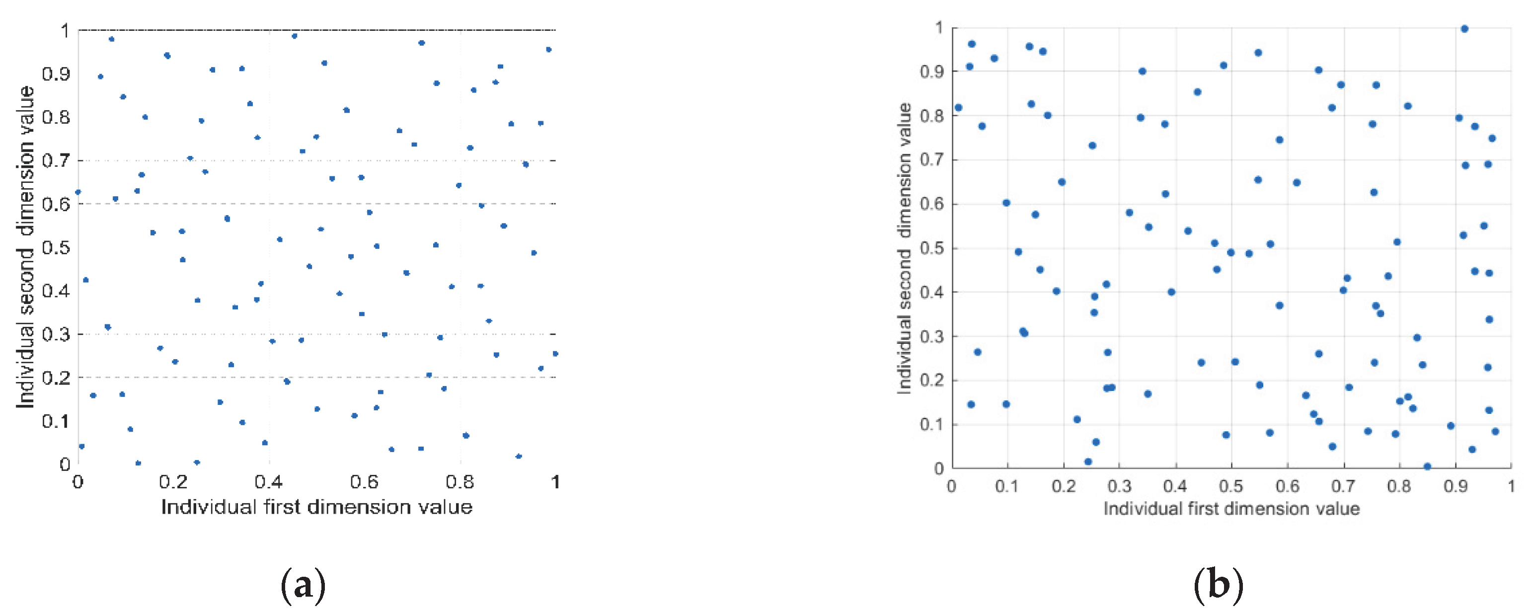
Figure 2.
Change in disturbance radius.
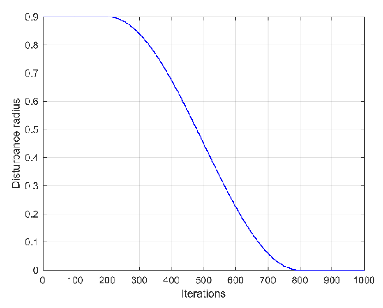
Figure 3.
MIDBO algorithm flowchart.

Figure 4.
Iteration diagram of the CEC2022 test function under different functions: (a) F1, (b) F2, (c) F3, (d) F4, (e) F5, (f) F6, (g) F7, (h) F8, (i) F9, (j) F10, (k) F11, (l) F12.
Figure 4.
Iteration diagram of the CEC2022 test function under different functions: (a) F1, (b) F2, (c) F3, (d) F4, (e) F5, (f) F6, (g) F7, (h) F8, (i) F9, (j) F10, (k) F11, (l) F12.
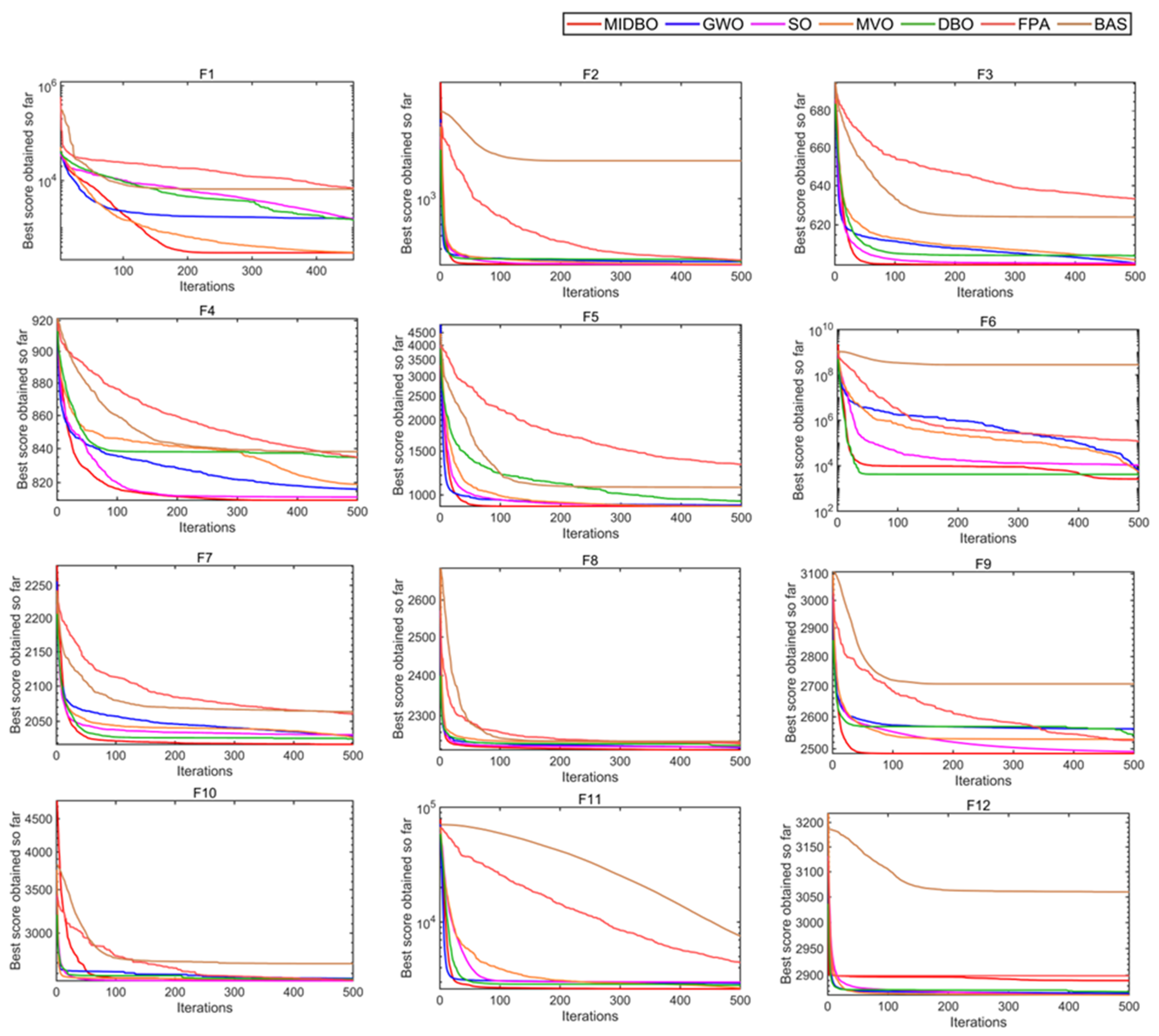
Figure 5.
Iteration diagram of improved algorithm CEC2022 test function under different functions: (a) F1, (b) F2, (c) F3, (d) F4, (e) F5, (f) F6, (g) F7, (h) F8, (i) F9, (j) F10, (k) F11, (l) F12.
Figure 5.
Iteration diagram of improved algorithm CEC2022 test function under different functions: (a) F1, (b) F2, (c) F3, (d) F4, (e) F5, (f) F6, (g) F7, (h) F8, (i) F9, (j) F10, (k) F11, (l) F12.
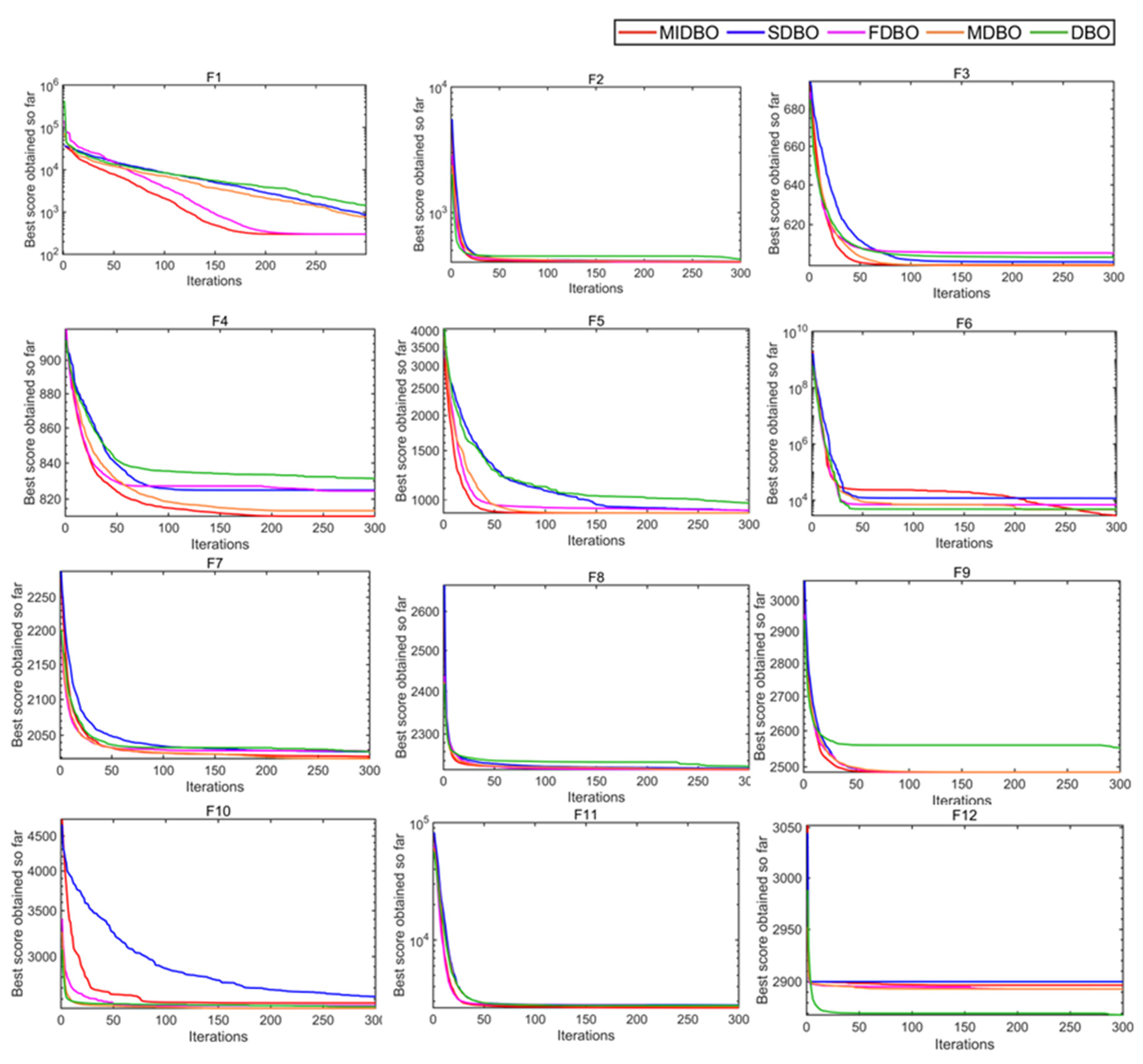
Figure 6.
When n = 4, 6, 8, 12, the effect of Camera graphic segmentation.
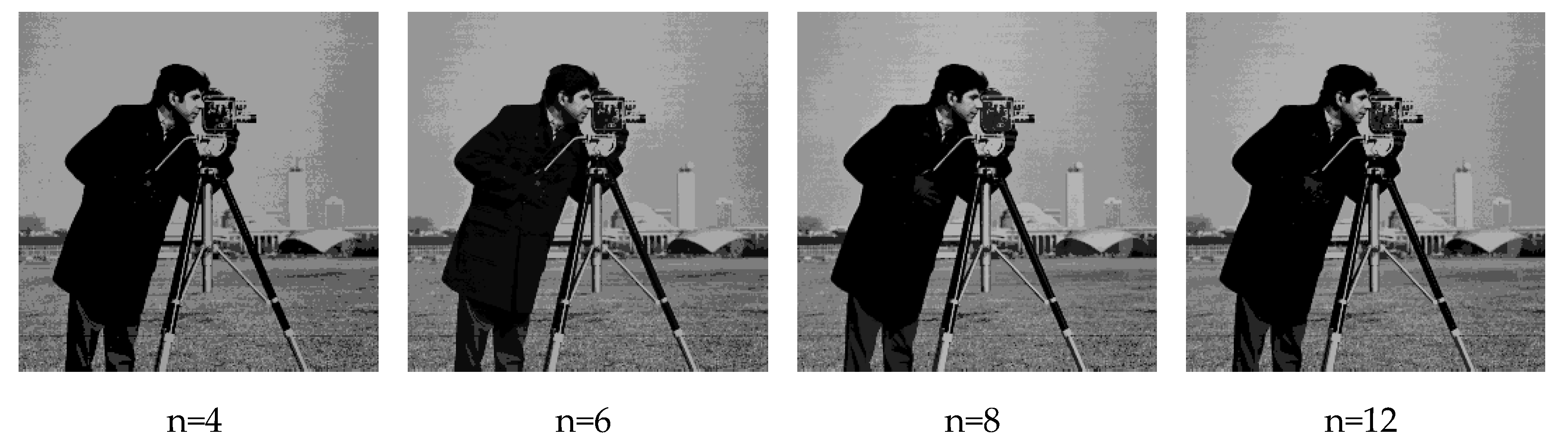
Figure 7.
When n = 4, 6, 8, 12, the effect of Plane graphic segmentation.
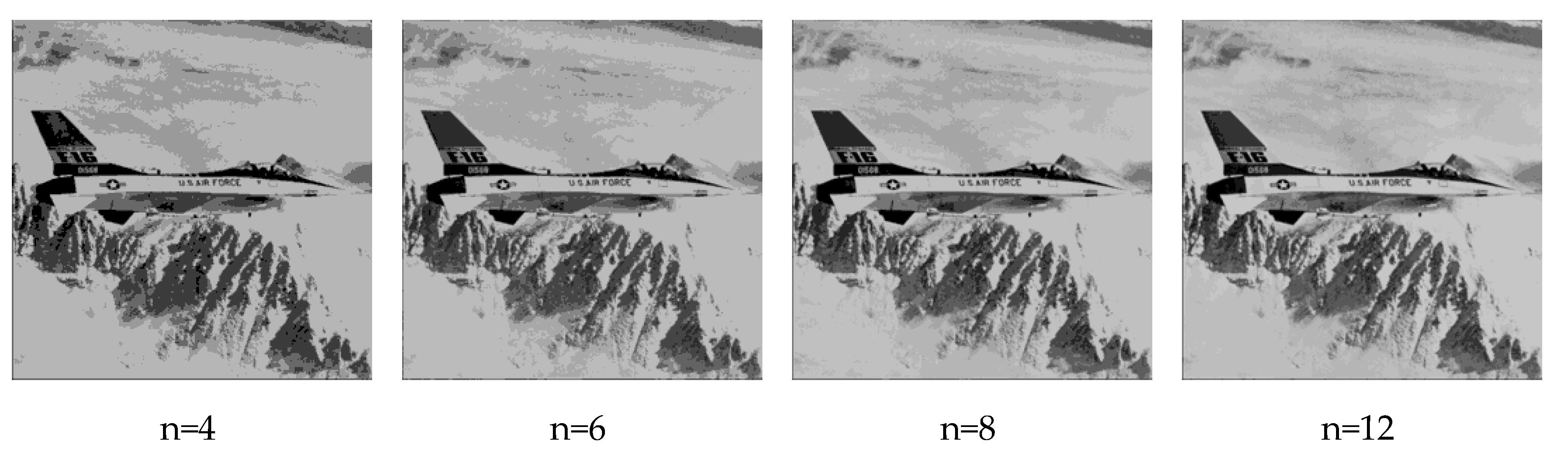

Table 1.
Test function information.
| Function name | No. | Functions | |
|---|---|---|---|
| Unimodal Function |
1 | Shifted and full Rotated Zakharov Function | 300 |
| Basic Functions |
2 | Shifted and fully rotated Rosenbrock’s Function | 400 |
| 3 | Shifted and full Rotated Expanded Schaffer’s f6 Function | 600 | |
| 4 | Shifted and full Rotated Non-Continuous Rastrigin’s Function | 800 | |
| 5 | Shifted and full Rotated Levy Function | 900 | |
| Hybrid Functions |
6 | Hybrid Function 1 (N = 3) | 1800 |
| 7 | Hybrid Function 2 (N = 6) | 2000 | |
| 8 | Hybrid Function 3 (N = 5) | 2200 | |
| Composition Functions |
9 | Composition Function 1 (N = 5) | 2300 |
| 10 | Composition Function 2 (N = 4) | 2400 | |
| 11 | Composition Function 3 (N = 5) | 2600 | |
| 12 | Composition Function 4 (N = 6) | 2700 | |
Table 2.
CEC2022 Test Function 2 Results.
| Func. | Dim. | Indi. | MIDBO | GWO | SO | MVO | DBO | FPA | BAS | ||||
|---|---|---|---|---|---|---|---|---|---|---|---|---|---|
| F1 | 10 | Best | 300 | 345.3092 | 318.3107 | 300.0108 | 300 | 1001.255 | 1988.901 | ||||
| Std | 1.98E-13 | 1607.695 | 1087.288 | 0.03542 | 668.6178 | 2912.941 | 2071.044 | ||||||
| Mean | 300 | 1737.622 | 1262.631 | 300.0489 | 576.2715 | 5345.38 | 52.18.876 | ||||||
| F2 | 10 | Best | 400.1135 | 402.0848 | 400.0849 | 400.0387 | 400.0513 | 412.3448 | 629.5263 | ||||
| Std | 1.9476 | 23.1172 | 2.7056 | 12.5278 | 27.8919 | 9.1908 | 700.6967 | ||||||
| Mean | 401.6285 | 422.3099 | 404.0562 | 408.4185 | 419.7833 | 427.7779 | 1640.674 | ||||||
| F3 | 10 | Best | 600.0023 | 600.0828 | 600.6971 | 600.1822 | 600.1631 | 622.5199 | 611.012 | ||||
| Std | 0.5624 | 0.5627 | 1.1817 | 3.1383 | 5.0678 | 6.0866 | 8.3312 | ||||||
| Mean | 600.2731 | 600.5877 | 601.4654 | 602.0208 | 605.0228 | 633.1458 | 625.2483 | ||||||
| F4 | 10 | Best | 803.9798 | 804.1978 | 804.5676 | 808.956 | 810.7761 | 825.7786 | 819.7244 | ||||
| Std | 3.2685 | 0.5627 | 3.8431 | 11.2878 | 11.9834 | 4.9787 | 10.0399 | ||||||
| Mean | 808.5898 | 814.9306 | 810.357 | 823.2847 | 830.4716 | 835.568 | 839.1543 | ||||||
| F5 | 10 | Best | 900 | 900.1186 | 900.2933 | 900.0014 | 900.4638 | 1031.73 | 917.2049 | ||||
| Std | 0.0693 | 11.5821 | 8.3399 | 0.5909 | 26.5231 | 190.3919 | 87.0764 | ||||||
| Mean | 900.0507 | 905.1358 | 902.081 | 900.2423 | 926.039 | 1309.526 | 1065.214 | ||||||
| F6 | 10 | Best | 1803.5 | 1913.462 | 2065.397 | 1967.53 | 2138.233 | 9387.876 | 1848.408 | ||||
| Std | 239.1878 | 2319.833 | 3568.985 | 2393.873 | 1934.538 | 77376.31 | 2374.0863 | ||||||
| Mean | 1959.214 | 6110.882 | 7523.001 | 4186.314 | 5370.294 | 93423.94 | 4431.624 | ||||||
| F7 | 10 | Best | 2000.624 | 2005.941 | 2006.657 | 2017.7 | 2001.62 | 2044.477 | 2033.249 | ||||
| Std | 6.9295 | 10.0903 | 5.6428 | 28.1291 | 12.4153 | 8.8352 | 20.824 | ||||||
| Mean | 2020.596 | 2009.362 | 2028.812 | 2031.539 | 2027.971 | 2058.375 | 2060.787 | ||||||
| F8 | 10 | Best | 2200.159 | 2210.208 | 2205.768 | 2221.976 | 2220.567 | 2228.081 | 2217.587 | ||||
| Std | 7.5046 | 4.4646 | 5.6428 | 42.2656 | 4.1016 | 3.6022 | 16.1669 | ||||||
| Mean | 2218.1 | 2223.985 | 2223.56 | 2243.028 | 2225.904 | 2234.494 | 2232.519 | ||||||
| F9 | 10 | Best | 2485.502 | 2529.293 | 2488.065 | 2529.289 | 2529.284 | 2494.609 | 2656.135 | ||||
| Std | 1.53E-12 | 41.98763 | 2.2671 | 26.8173 | 34.1851 | 29.5603 | 37.0427 | ||||||
| Mean | 2485.502 | 2562.242 | 2491.389 | 2534.23 | 2549.373 | 2524.606 | 2722.926 | ||||||
| F10 | 10 | Best | 2403.54 | 2500.22 | 2422.562 | 2500.203 | 2500.381 | 2508.011 | 2502.788 | ||||
| Std | 63.4296 | 83.6739 | 59.7726 | 135.8494 | 62.1079 | 124.0359 | 301.3793 | ||||||
| Mean | 2560.141 | 2561.251 | 2527.178 | 2590.259 | 2539.257 | 2576.715 | 2694.086 | ||||||
| F11 | 10 | Best | 2600 | 2731.359 | 2993.586 | 2603.593 | 2600 | 3175.546 | 4039.877 | ||||
| Std | 54.0871 | 93.1558 | 64.0764 | 203.5316 | 243.9764 | 553.838 | 1687.189 | ||||||
| Mean | 2623.544 | 2959.11 | 3016.3085 | 2751.437 | 2853.169 | 4349.104 | 7289.763 | ||||||
| F12 | 10 | Best | 2846.017 | 2862.752 | 2855.21 | 2858.638 | 2863.159 | 2864.106 | 2946.976 | ||||
| Std | 13.5219 | 4.8807 | 4.7232 | 1.4237 | 16.3449 | 7.6466 | 64.0214 | ||||||
| Mean | 2896.449 | 2866.59 | 2864.581 | 2863.478 | 2872.096 | 2897.395 | 3069.284 | ||||||
*Note: In the Table 2, Func. denotes Function, Dim. denotes Dimension, Indi. denotes Indicators.
Table 3.
Wilcoxon rank sum test results.
| Function | GWO | SO | MVO | DBO | FPA | BAS |
|---|---|---|---|---|---|---|
| F1 | 5.5321E-74 | 5.5321E-74 | 5.5321E-74 | 5.5321E-74 | 5.5321E-74 | 5.5321E-74 |
| F2 | 7.3994E-62 | 7.3994E-62 | 7.3994E-62 | 7.3994E-62 | 7.3994E-62 | 7.3994E-62 |
| F3 | 1.8973E-55 | 1.8974E-55 | 1.8974E-55 | 1.8974E-55 | 1.8974E-55 | 1.8974E-55 |
| F4 | 1.3598E-83 | 1.3598E-83 | 1.3598E-83 | 1.3598E-83 | 1.3598E-83 | 1.3598E-83 |
| F5 | 5.4567E-59 | 5.4567E-59 | 5.4567E-59 | 5.4567E-59 | 5.4567E-59 | 5.4567E-59 |
| F6 | 4.8442E-69 | 4.8442E-69 | 4.8442E-69 | 4.8442E-69 | 4.8442E-69 | 4.8442E-69 |
| F7 | 1.0967E-81 | 1.0967E-81 | 1.0967E-81 | 1.0967E-81 | 1.0967E-81 | 1.0967E-81 |
| F8 | 1.4881E-45 | 1.4881E-45 | 1.4881E-45 | 1.4881E-45 | 1.4881E-45 | 1.4881E-45 |
| F9 | 9.7451E-79 | 9.7451E-79 | 9.7451E-79 | 9.7451E-79 | 9.7451E-79 | 9.7451E-79 |
| F10 | 7.2771E-47 | 7.2771E-47 | 7.2771E-47 | 7.2771E-47 | 7.2771E-47 | 7.2771E-47 |
| F11 | 8.9699E-68 | 8.9699E-68 | 8.9699E-68 | 8.9699E-68 | 8.9699E-68 | 8.9699E-68 |
| F12 | 4.9385E-76 | 4.9385E-76 | 4.9385E-76 | 4.9385E-76 | 4.9385E-76 | 4.9385E-76 |
Table 4.
Comparison of optimization results for multiple improvement strategies.
| Function | Indicators | DBO | SDBO | FDBO | MDBO | MIDBO |
|---|---|---|---|---|---|---|
| F1 | Best | 322.2929 | 321.6293 | 300.3925 | 301.7422 | 300 |
| 300 | Mean | 483.0199 | 320.859 | 300.0004 | 308.6264 | 300 |
| Std | 246.5947 | 86.5498 | 0.0014611 | 31.9939 | 2.9363E-13 | |
| F2 | Best | 400.5527 | 400.049 | 400.3191 | 400.0393 | 400.0249 |
| 400 | Mean | 427.8402 | 404.5403 | 409.3614 | 407.4164 | 404.0657 |
| Std | 32.4372 | 2.572 | 16.8402 | 15.4863 | 2.5672 | |
| F3 | Best | 600.0179 | 600.0032 | 600.2285 | 600.0002 | 600.0001 |
| 600 | Mean | 607.6264 | 601.6133 | 604.9408 | 600.0765 | 600.0241 |
| Std | 8.116 | 2.2539 | 6.1834 | 0.2824 | 0.53487 | |
| F4 | Best | 810.9445 | 804.9748 | 808.9546 | 804.2699 | 804.1748 |
| 800 | Mean | 832.6764 | 825.6367 | 826.1342 | 813.5914 | 810.2481 |
| Std | 11.3855 | 10.6511 | 10.4774 | 5.8411 | 3.2546 | |
| F5 | Best | 900.0919 | 900.0079 | 900.0895 | 900 | 900 |
| 800 | Mean | 940.6964 | 924.9668 | 940.7126 | 900.0776 | 900.1898 |
| Std | 74.988 | 37.9901 | 68.5948 | 0.07706 | 0.2028 | |
| F6 | Best | 1883.3084 | 1881.6132 | 1819.4202 | 1884.9456 | 1814.0878 |
| 1800 | Mean | 5009.0288 | 14100.7001 | 7991.9951 | 5909.5978 | 2325.9438 |
| Std | 2269.6112 | 12613.1149 | 11537.774 | 4289.004 | 809.6063 | |
| F7 | Best | 2019.6384 | 2003.5749 | 2001.3025 | 2000.9953 | 2004.9748 |
| 2000 | Mean | 2029.484 | 2028.1521 | 2029.8622 | 2021.676 | 2021.2029 |
| Std | 15.6998 | 12.9299 | 13.6341 | 6.6804 | 5.3636 | |
| F8 | Best | 2220.1304 | 2220.2234 | 2203.6886 | 2203.9429 | 2200.5355 |
| 2200 | Mean | 226.1435 | 2222.3121 | 2220.1613 | 2222.014 | 2219.2819 |
| Std | 4.9128 | 6.3306 | 3.7943 | 5.173 | 2.0135 | |
| F9 | Best | 2529.2844 | 2485.5017 | 2485.5017 | 2485.5017 | 2485.5017 |
| 2300 | Mean | 2542.2794 | 2492.6967 | 2485.5018 | 2485.502 | 2488.4953 |
| Std | 24.9954 | 16.3847 | 39.4088 | 0.0005607 | 0.000216 | |
| F10 | Best | 2500.3708 | 2500.4565 | 2455.0457 | 2450.2654 | 2400.2008 |
| 2400 | Mean | 2556.2397 | 2626.9604 | 2573.4804 | 2520.514 | 2558.5539 |
| Std | 64.9599 | 125.0734 | 64.4409 | 52.7332 | 57.5874 | |
| F11 | Best | 2600 | 2600 | 2600 | 2600 | 2600 |
| 2600 | Mean | 2845.5632 | 2791.4051 | 2744.7952 | 2703.8944 | 2620.3293 |
| Std | 230.5968 | 154.3065 | 159.0115 | 158.1639 | 51.9195 | |
| F12 | Best | 2861.1537 | 2846.7353 | 2847.6924 | 2846.6503 | 2900.0014 |
| 2700 | Mean | 2869.9378 | 2898.2265 | 2893.4513 | 2887.7465 | 2900.002 |
| Std | 15.2099 | 9.7251 | 17.0214 | 22.5967 | 0.0001819 |
Table 5.
PSNR values for multi-threshold image segmentation using various algorithms when m = 4, 6, 8, and 12.
Table 5.
PSNR values for multi-threshold image segmentation using various algorithms when m = 4, 6, 8, and 12.
| Image | Threshold quantity | MIDBO | DBO | FPA | SO | GWO | WOA |
|---|---|---|---|---|---|---|---|
| Camera | 4 | 22.30 | 22.27 | 21.96 | 21.99 | 19.96 | 22.14 |
| 6 | 24.80 | 24.34 | 23.76 | 24.09 | 21.05 | 24.29 | |
| 8 | 26.49 | 24.49 | 25.74 | 26.19 | 23.60 | 26.40 | |
| 12 | 28.57 | 28.30 | 26.97 | 28.86 | 25.03 | 28.85 | |
| Pepper | 4 | 21.01 | 20.82 | 20.01 | 20.93 | 16.90 | 20.81 |
| 6 | 24.03 | 22.62 | 22.52 | 23.16 | 21.37 | 23.10 | |
| 8 | 25.58 | 24.76 | 23.58 | 24.86 | 20.32 | 24.41 | |
| 12 | 28.91 | 26.25 | 27.29 | 27.33 | 25.40 | 26.17 | |
| Plane | 4 | 22.00 | 21.94 | 21.19 | 21.99 | 18.52 | 21.86 |
| 6 | 25.15 | 25.01 | 23.53 | 25.08 | 21.50 | 21.88 | |
| 8 | 26.95 | 26.80 | 26.49 | 26.65 | 25.72 | 26.75 | |
| 12 | 30.20 | 27.60 | 27.88 | 28.64 | 25.45 | 29.06 | |
| House2 | 4 | 22.91 | 21.10 | 21.96 | 21.29 | 20.10 | 22.53 |
| 6 | 24.72 | 24.55 | 24.32 | 23.46 | 23.15 | 23.50 | |
| 8 | 27.66 | 25.01 | 25.34 | 26.58 | 25.12 | 26.24 | |
| 12 | 29.62 | 29.09 | 28.32 | 29.54 | 25.73 | 27.46 |
Table 6.
SSIM values for multi-threshold image segmentation using various algorithms when m = 4, 6, 8, and 12.
Table 6.
SSIM values for multi-threshold image segmentation using various algorithms when m = 4, 6, 8, and 12.
| Image | Threshold quantity | MIDBO | DBO | FPA | SO | GWO | WOA |
|---|---|---|---|---|---|---|---|
| Camera | 4 | 0.69 | 0.70 | 0.68 | 0.68 | 0.69 | 0.69 |
| 6 | 0.73 | 0.73 | 0.72 | 0.71 | 0.64 | 0.72 | |
| 8 | 0.87 | 0.82 | 0.76 | 0.76 | 0.87 | 0.76 | |
| 12 | 0.89 | 0.83 | 0.76 | 0.92 | 0.73 | 0.89 | |
| Pepper | 4 | 0.73 | 0.73 | 0.71 | 0.73 | 0.67 | 0.71 |
| 6 | 0.80 | 0.77 | 0.78 | 0.78 | 0.75 | 0.78 | |
| 8 | 0.85 | 0.83 | 0.80 | 0.84 | 0.76 | 0.82 | |
| 12 | 0.91 | 0.88 | 0.89 | 0.90 | 0.86 | 0.86 | |
| Plane | 4 | 0.83 | 0.82 | 0.82 | 0.83 | 0.71 | 0.83 |
| 6 | 0.88 | 0.88 | 0.85 | 0.87 | 0.78 | 0.83 | |
| 8 | 0.90 | 0.90 | 0.89 | 0.90 | 0.88 | 0.89 | |
| 12 | 0.94 | 0.91 | 0.92 | 0.93 | 0.87 | 0.92 | |
| House2 | 4 | 0.80 | 0.77 | 0.80 | 0.86 | 0.61 | 0.78 |
| 6 | 0.82 | 0.85 | 0.83 | 0.81 | 0.79 | 0.84 | |
| 8 | 0.89 | 0.84 | 0.85 | 0.85 | 0.84 | 0.86 | |
| 12 | 0.89 | 0.89 | 0.90 | 0.89 | 0.85 | 0.86 |
Table 7.
FSIM values for multi-threshold image segmentation using various algorithms when m = 4, 6, 8, and 12.
Table 7.
FSIM values for multi-threshold image segmentation using various algorithms when m = 4, 6, 8, and 12.
| Image | Threshold quantity | MIDBO | DBO | FPA | SO | GWO | WOA |
|---|---|---|---|---|---|---|---|
| Camera | 4 | 0.86 | 0.86 | 0.85 | 0.84 | 0.85 | 0.85 |
| 6 | 0.90 | 0.90 | 0.89 | 0.89 | 0.81 | 0.89 | |
| 8 | 0.91 | 0.87 | 0.93 | 0.93 | 0.83 | 0.93 | |
| 12 | 0.94 | 0.94 | 0.93 | 0.94 | 0.90 | 0.94 | |
| Pepper | 4 | 0.77 | 0.77 | 0.76 | 0.76 | 0.72 | 0.77 |
| 6 | 0.83 | 0.82 | 0.81 | 0.83 | 0.79 | 0.82 | |
| 8 | 0.87 | 0.85 | 0.83 | 0.86 | 0.79 | 0.85 | |
| 12 | 0.92 | 0.89 | 0.90 | 0.91 | 0.87 | 0.88 | |
| Plane | 4 | 0.84 | 0.85 | 0.83 | 0.84 | 0.74 | 0.84 |
| 6 | 0.90 | 0.90 | 0.86 | 0.90 | 0.82 | 0.84 | |
| 8 | 0.92 | 0.92 | 0.92 | 0.92 | 0.91 | 0.92 | |
| 12 | 0.96 | 0.93 | 0.94 | 0.94 | 0.89 | 0.95 | |
| Hoe2 | 4 | 0.82 | 0.81 | 0.82 | 0.81 | 0.76 | 0.80 |
| 6 | 0.87 | 0.86 | 0.83 | 0.83 | 0.83 | 0.84 | |
| 8 | 0.91 | 0.87 | 0.88 | 0.89 | 0.87 | 0.88 | |
| 12 | 0.94 | 0.94 | 0.91 | 0.94 | 0.89 | 0.89 |
Disclaimer/Publisher’s Note: The statements, opinions and data contained in all publications are solely those of the individual author(s) and contributor(s) and not of MDPI and/or the editor(s). MDPI and/or the editor(s) disclaim responsibility for any injury to people or property resulting from any ideas, methods, instructions or products referred to in the content. |
© 2026 by the authors. Licensee MDPI, Basel, Switzerland. This article is an open access article distributed under the terms and conditions of the Creative Commons Attribution (CC BY) license (http://creativecommons.org/licenses/by/4.0/).
Copyright: This open access article is published under a Creative Commons CC BY 4.0 license, which permit the free download, distribution, and reuse, provided that the author and preprint are cited in any reuse.


