
Submitted:
31 July 2025
Posted:
31 July 2025
You are already at the latest version
Abstract
In image segmentation, local thresholding algorithms may yield more accurate and robust results since they are based on the features of images. Therefore, the common patterns exhibit in the same image category is crucial to improve the quality of segmentation results. In present paper, a new local thresholding algorithm that using gradient aided histogram is proposed to process the images that have apparent texture or periodical structure. It is found that clustering pixels with similar gray-level gradient plays an important role for the multi-level image segmentation. The famous global thresholding algorithms, such as Kapur and Otsu, are adopted to make the comparison. The results are quantitatively illustrated in terms of PSNR (Peak Signal-to-Noise Ratio) and FSIM (Feature Similarity Index). It is shown that the proposed algorithm can effectively recognize the common features of the images that belong to the same category, and maintain the stable performances when the number of threshold increases. Furthermore, the processing time of present algorithm is competitive to those of other algorithms, which shows the potential application in real time scenes.
Keywords:
local thresholding method
; image segmentation
; Otsu method
; 2-D Gradient orientation histogram
1. Introduction
With the popularization of imaging devices, the demand for image data analyses has significantly increased. As a result, image processing has become an essential component in various applications, with image segmentation serving as a fundamental and crucial step. This step divides an image into multiple regions based on its characteristics such as color, brightness, contour, and semantics. The technique has been extensively applied in numerous fields [1,2,3,4,5] and continues to evolve. Technically, the threshold-based image segmentation has become the most frequently used method due to its simplicity, efficiency, and stability [6].
Threshold-based segmentation can generally be categorized into global and local thresholding methods. The global methods apply a single or multiple thresholds to segment the entire image, offering computational efficiency and algorithmic simplicity. In 1985, Kapur [7] proposed the maximum Shannon entropy threshold method. This method selects an optimal threshold based on the image’s one-dimensional (1-D) gray-level histogram, and then segment it into foreground and background regions. Another typical global thresholding is Otsu’s method [8], which determines the optimal threshold by maximizing the between-class variance of the foreground and background. Both approaches are automatic thresholding algorithms that based on the 1-D gray-level histogram of an image. However, the 1-D histogram only counts the number of pixels that have the same gray-level values without considering the association information between different pixels, such as the spatial distribution information of pixels in the image. If the spatial correlation information between different pixels is nontrivial, the above mentioned global algorithms may not perform optimally [7]. To address the limitations of 1-D histogram, Abutaleb [9] proposed a two-dimensional (2-D) histogram in 1989, which incorporates both the gray values of pixels and their local average gray values. This approach extended Kapur’s method to 2-D histogram, determining the optimal threshold vector by maximizing the sum of the 2-D Shannon entropy of the foreground and background regions, particularly performs well in images with low signal-to-noise ratios (SNR). Since then, many other 2-D histogram-based thresholding methods have been proposed by utilizing different objective function [10,11,12,13,14]. However, the enhanced accuracy comes at the cost of increased computational complexity. The computation time grows exponentially as the number of thresholds increases. Furthermore, traditional 2-D entropy methods tend to recognize the pixels located on the main diagonal of the 2-D histogram, which may result in the loss of edge information [15].
While global thresholding techniques are efficient and straightforward, local techniques offer higher segmentation accuracy [16,17]. The local thresholding methods first divide the image into several independent regions that satisfy a given homogeneity criterion [18,19], and these regions are segmented by using region-specific thresholds subsequently. These methods incorporate pixel-wise correlation information [20,21,22], including backscatters and texture measures [23], statistical measures like mean intensity and standard deviation [24], as well as color and distance [25]. The local thresholding methods employ feature-based preprocessing prior to segmentation, and this hierarchical approach effectively reduces the segmentation error, enhances noise resistance, and achieves superior image quality.
Therefore, incorporating additional image feature information can significantly enhance segmentation accuracy. Among these features, texture information [26], which partially reflects edge characteristics and can be quantified through gradient-based measurements, is widely utilized in image processing applications [27,28,29,30,31,32,33,34,35,36,37,38,39]. Crucially, such edge information of an image captures the outlines, structures, and transitions of objects in the image. It typically corresponds to regions where the gray values changes dramatically in the image, and plays an important role in separating different areas or objects. The extraction of texture information would be helpful to keep the predominant patterns of an image. Specifically, for texture-rich images, proper utilization of such information may play a crucial role in segmentation tasks. Therefore, a unified approach that can effectively act on different texture-rich image categories is important to reveal the relationships between texture patterns and pixel gradient clustering.
In this paper, we propose a local thresholding method that utilizes a gradient orientation histogram to extract local texture features from images. This method clusters pixels with similar gradient directions into distinct subsets using a 2-D gradient orientation histogram, which incorporates both the gray values of pixels and their gradient orientations. Local thresholding is then applied to each subset. The remainder to this paper is organized as follows. Section 2 briefly introduces the pixel-wise gradient orientation and reviews both the 1-D Otsu method and 2-D Otsu method. Section 3 presents the construction of the 2-D gradient orientation histogram and the process of the local threshoding method. Section 4 reports on the experimental results from two datasets and discussions. In Section 5, the conclusions are presented.
2. Related Works
2.1. Pixel-Wise Gradient Orientation
The pixel-wise gradient orientation [40,41,42,43] serves as an effective descriptor for local structural features, particularly in texture characterization. One of the ways to generate it is as follows, for a pixel located at position , its gradient along the vertical and horizontal axes can be respectively defined as:
where represents the gray-level value of pixel at ,
Then the orientation of this pixel can be calculated by:
where the domain of is .
2.2. 1-D Otsu’s Method
Define the range of gray levels in a given image of size as , where L represents the maximum gray-level of the image, such as 256. Then the gray-level histogram of the image can be computed by the probability distribution:
where is the number of pixels that gray-level values equal to i.
Assuming that the gray-level histogram of the image is divided into two classes and by a threshold at level t, then the probabilities of class occurrences and the class mean gray-level values are given by:
and
Thus, the entire image’s mean gray-level value can be obtained as follows:
The between-class variance can be represented by:
The optimal threshold can be obtained by maximizing Equation (8), i.e.,
Based on a set of thresholds , the image can be divided into classes, denoted as , and the mean gray-level values are defined as:
where
Then the between-class variance can be calculated by:
The optimal threshold vector can be obtained by maximizing the multi between-class variance,
2.3. 2-D Otsu’s Method
For 2-D Otsu method [44], for a given image of size , the value of is ranging from 0 to . At position , the average gray value of its local neighborhood can be obtained via:
where denotes the integer part of , n is the size of the local square centered at . Then the 2-D gray-level histogram of the image is given by:
where returns 1 when and , else returns 0. Using a threshold vector to partition the histogram into two classes and (background and objects), then the probabilities of class occurrence are given by:
The corresponding class mean levels are:
The total mean level vector of the 2-D histogram is:
The between-class variance matrix is defined as:
The trace of can be used to measure the between-class variance, it is computed by:
where
Then the optimal threshold vector is determined by:
3. Proposed Method
Traditional 2-D entropy threshold methods may cause the loss of a considerable number of pixels, leading to the loss of nontrivial edge information. Consequently, a novel algorithm is proposed to avoid such cases so that the segmentation accuracy can be improved. For a texture-rich image, the edge pattern is deeply related with the gradient of pixels’ gray-level. Therefore, a 2-D gradient orientation histogram is adopted to cluster the image pixels into distinct regions. And the local thresholding to each region demonstrates the advantages.
3.1. Construction of 2-D Gradient Orientation Histogram
For a pixel located at position in a given image of size , its gray-level gradient orientation with respect to the horizontal axis is:
where denotes the transform of the radian angle to degree. and can be calculated by Equation (1) and Equation (2), and the domain of is . The pixel’s gray-level value, , and the gradient orientation can be adopted to construct the 2-D gradient orientation histogram by
The 2-D probability distribution is determined by normalization of Equation (24),
3.2. Main Step of Segmentation
For a digital image of size , the normalized 2-D gradient orientation histogram can be obtained via Equation (25). Different from Equation (15), the distribution of is not concentrated at the main diagonal of the 2-D histogram, as it is shown in Figure 1. The probability distribution of each gradient orientation angle in the image can be obtained by:
where k ranging from . Using Otsu’s method with a set of thresholds , the distribution of Equation (26) can be segmented into three distinct parts, denoted as , with each part comprising pixels that have similar gradient orientation angles. After normalization, the gray-level probability distribution of three classes are respectively defined as:
where the cumulative probabilities of three classes are defined as:
The mean gradient orientation angles of three classes are as follows:
The entire image’s mean gradient orientation angle can be obtained by:
The between-class variance of orientation can be represented by:
Maximizing the objective function yields the optimal set of thresholds as follows:
Using the optimal threshold , the 2-D gradient orientation histogram is clustered into three parts with the largest between-class variance. Each part contains pixels with similar gradient orientation information. Figure 2 shows an example, with the optimal vector , the pixels of each gradient orientation part can be sorted by gray-level value and yields the corresponding histogram.
After clustering the image, the Otsu’s method mentioned in Section 2.2 is used to perform local thresholding segmentation on the three regions. The three segmentation results are then combined to obtain the final segmentation result. Figure 3 illustrates the overall segmentation process.
3.3. Image Test Sets and Quality Evaluation Parameters
Image texture not only characterizes local structural patterns but also effectively captures inter-object boundary information. Due to its important role in object recognition, texture features have been widely employed in image analysis. To further show the relationship between texture information and image segmentation, images with diverse texture characteristics are adopted in the experiments. Figure 4 displays three images with obvious texture features from the MATLAB image library, with resolutions of (a),(b) and (c).
Beside Figure 4, more real-world images from various scenes are essential to test the proposed algorithm. The Describable Textures Dataset (DTD, R1.0.1) [45] is an image dataset consisting of 47 different categories of real-world texture images, with each category named by an adjective. It is designed as a public benchmark and can be used to study the problem of extracting semantic properties of textures and patterns. In this paper, the segmentation experiment employs 81 ’woven’, 119 ’lacelike’, 107 ’pitted’, and 119 ’blotchy’ images. Here are a few examples from this dataset (Figure 5).
To evaluate the effectiveness of the local thresholding method proposed above, we adopt PSNR (Peak Signal-to-Noise Ratio) and FSIM (Feature Similarity Index) as quality indices. PSNR [46] represents the ratio of the peak signal to the noise. As it can precisely measure the difference between the input image and the output image, it is currently the most frequently used objective metric for evaluating image quality. A higher PSNR value indicates less distortion in the output image and better segmentation quality. It is defined as:
where the is the mean squared error between the input image and the output image, and L is the maximum gray-level value in the image, usually 255. can be written as:
where is the size of the image, and represent the input image and the output image, respectively.
FSIM [47] is proposed based on the principle that human visual system understands an image mainly according to its low-level features. It is utilized to measure the similarity between two images based on phase congruence (PC) and image gradient magnitude (GM). Here, PC serves as a dimensionless indicator of the importance of local structures and is used as the primary feature in the FSIM. GM acts as the secondary feature in FSIM. Both features playing complementary roles in characterizing the local quality of an image. FSIM is defined as:
where means the whole image spatial domain, is the local similarity at pixel x, is the maximum PC value at pixel x. Please refer to [47] for more details about and .
4. Experimental Results and Discussions
To demonstrate the performance of the proposed method, we tested images from MATLAB image library (Figure 4) and the DTD dataset (Figure 5). The Kapur method [48], 1-D Otsu method [49], 2-D Otsu method, and the proposed method were applied to segment these images, with the number of thresholds set to 2, 3, 4, and 5.
4.1. Algorithm Performance and Computational Cost
Figure 6 demonstrates the two-level thresholding performances for three images of Figure 4. It is found that the proposed method keeps more details than others, and can avoid lots of mis-segmentations. Notably, this advantage keeps with the increasing number of threshold and can be quantitatively illustrated. Table 1 presents the PSNR and FSIM results at different threshold levels for these three images. In each row, the maximum PSNR and FSIM values (with bold font) indicate that the corresponding method is the most suitable one for the image listed at the beginning of the row. The proposed method achieved the best PSNR and FSIM values for all three texture-rich images across all threshold levels. It performs better than 1-D histogram-based methods because it incorporates more pixel-wise correlation information for segmentation. Meanwhile, traditional 2-D methods neglect off-diagonal pixels’ contributions, leading to image information loss. In contrast, the proposed method utilizes gradient information from all pixels for segmentation, thereby achieving superior performance. This also indicates that, compared to the 2-D average gray values histogram, the gradient aided histogram is more effective in analyzing the texture features of these images.
Table 2 presents the comparative computational time costs across different methods. All algorithms were implemented in Python and executed on a workstation equipped with dual Intel Xeon Gold 6268CL processors (2.80 GHz, 28 cores total) and 256 GB DDR4 RAM (2666 MHz). To ensure fair comparison, all methods were restricted to single-thread execution.
It is shown that, the proposed method obtained more precise segmentation results while requiring less computational time than 2-D Otsu method. It should be noted that the proposed method can adopt multiprocessing computation for segmenting the three clustered regions. So, compared with traditional 1-D methods, it only incurs additional computational cost for constructing 2-D gradient orientation histogram and the corresponding pixels’ clustering. It achieves both stable segmentation accuracy improvement and low computational consumption, showing the potential application in real time scenes.
4.2. Consistency of Algorithm Performance with Increasing Threshold
To further validate the effectiveness of the proposed method, we applied the above four methods to perform 2-level, 3-level, 4-level and 5-level thresholding on images from the DTD dataset mentioned in Section 3.3.
Figure 7 shows parts of the two-level thresholding results of some images. It is evident that for these four images, both 1-D Kapur and 2-D Otsu method yielded unsatisfactory segmentation results. Specifically, the 1-D Kapur method failed to capture the texture details, leading to difficulties in segmenting and preserving complex and diverse texture lines in the original images. The traditional 2-D method only considers pixels along the main diagonal of the histogram, which may result in the loss of important texture information. In comparison, the proposed method effectively preserved the texture lines and features from the original images.
In order to show the performances of these four algorithms objectively, different categories of DTD dataset are adopted to yield the comparisons. For example, the category named “woven” contains 81 images with similar texture structures. At given number of thresholds, each image yields 4 PSNR values by above four algorithms, respectively. The maximum PSNR value leads the count of corresponding algorithm increasing 1. It should be mentioned that two algorithms may occasionally reach the same maximum results. Therefore, the total count of 4 algorithms may slightly exceed the total number of images in the category. By the same way, the distributions of FSIM can be obtained. Table 3 presents the distributions of optimal PSNR and FSIM among four algorithms by using different image categories. For each image category, the bolded values represent the highest frequencies of reaching the optimal segmentation quality, which shows the superiority of corresponding algorithm.
For ‘woven’ category, the proposed method achieved optimal PSNR values over all 81 images at threshold levels 2 and 3, and obtained optimal FSIM values in approximately of cases. This demonstrates that the method maintains both high segmentation accuracy and effective preservation of texture details. With the increasing number of thresholds, such as 4 and 5, the optimal rate of PSNR for proposed algorithm is still dominant, and the corresponding optimal rate of FSIM slightly increases. This suggests that the proposed algorithm is stable in both segmentation accuracy and feature preservation for this image category with increasing threshold numbers.
In order to show the effectiveness of proposed algorithm, more image categories can be involved. For ‘lacelike’ category, the optimal PSNR rate of present algorithm is nearly at threshold levels 2 and 3. For ‘blotchy’ and ‘pitted’ categories, these rates are close to and , respectively. When the number of thresholds increases to 4 and 5, the optimal PSNR rates yielded by different image categories keep unchanged within a small interval of fluctuation. From Figure 5, we can see that the texture patterns among 4 image categories are quite different from each other. The proposed method reached an average optimal PSNR rate to , showing the powerful ability in texture pattern recognition. Regarding the optimal FSIM rate, the proposed method also keeps far larger than those of the other three typical algorithms. This superiority is unchanged in different image categories, with different threshold levels.
Actually, the superiority of proposed algorithm benefits from the pre-segmentation clustering based on local texture features, which depends closely on the pixels’ gradient orientation distribution. Although the four texture categories exhibit distinct visual characteristics, the proposed method consistently obtains satisfactory PSNR values across all categories. This shows that it effectively identifies texture patterns across diverse image categories, demonstrating strong scalability. FSIM evaluation shows that the proposed method demonstrates superior capability in preserving original image features across all categories. This validates that pixel gradient clustering contributes to analyzing complex texture distributions in different images. Furthermore, the method retains relatively stable performance with small fluctuations across different threshold levels, indicating good robustness and stability.
4.3. Comparative Analysis of Method Performance
The 2-D Otsu method yields unsatisfactory performance across all texture categories, with near-zero counts of images achieving maximum PSNR and FSIM values at all threshold levels. This likely stems from its threshold determination mechanism disregarding certain pixels, leading to significant loss of edge and feature information. Interestingly, while the 1-D Kapur method showed similarly poor PSNR results as 2-D Otsu method, it outperformed 2-D Otsu method in FSIM index. This can be attributed to its global thresholds selection based on all image pixels, which prevents lot feature loss and consequently preserves more texture characteristics in some images. The 1-D Otsu method achieved relatively better results for a small subset of images in both PSNR and FSIM. This may reflect better compatibility between the between-class variance maximization criterion and these texture images.
Clearly, traditional 1-D methods show limited performance for these texture-rich images. They fail to account for spatial correlations between pixels and utilize insufficient image information during threshold selection. However, 2-D Otsu method does not appear to perform significantly better, since the 2-D local average gray values histogram ignored pixels with high contrast to their surroundings. It is more suitable for low SNR scenarios. Consequently, its ability to extract texture information is weak, leading to suboptimal segmentation results.
The superior performance of the proposed method demonstrates the importance of texture information in segmentation tasks. It also confirms that gradient aided histogram serves as an effective descriptor for image texture patterns. This strongly validates the necessity of clustering pixels with similar gradient orientations for multi-level image segmentation.
5. Conclusions
In image segmentation, 2-D thresholding methods extract additional pixel-wise features, thereby overcoming the limitations of 1-D approaches in certain scenarios. This demonstrates that proper utilization of additional image features can effectively improve segmentation accuracy. But traditional 2-D entropy thresholding methods may inadvertently discard a significant proportion of pixels, thereby undermining the preservation of nontrivial edge details.
In this paper, we propose a new local thresholding algorithm to further study the importance of texture features in improving multi-level segmentation quality. To evaluate the performances, we compare our method with Kapur (1-D) and Otsu (1-D and 2-D) methods. Segmentation results are assessed by PSNR index. Experimental results demonstrate that our algorithm can accurately identify common patterns in texture-rich images. Specifically, when segmenting four texture categories of images with distinct characteristics from the DTD dataset, our method achieves significantly higher segmentation quality than other algorithms. This advantage stems from clustering pixels with similar gray-level gradient orientation before segmentation, which facilitates the algorithm’s understanding and analysis of feature distribution patterns in images. And the segmentation quality remains stable as the threshold level increases. Our method also shows superior performance in FSIM index, proving that the gradient aided histogram effectively captures texture information across different images. It can identify diverse texture patterns and periodical structures, preserving complex texture features in segmentation results. The performance sustains stability even as threshold levels increase, highlighting strong scalability. Notably, the improved performance comes with neglectable computational cost, demonstrating potential for real time applications.
Author Contributions
Conceptualization, C.O. and L.D.; methodology, C.O.; software, L.D.; validation, L.D. and K.Z.; formal analysis, C.O. and L.D.; investigation, L.D. and S.Z.; resources, M.H.; data curation, L.D.; writting—original draft preparation, L.D.; writing—review and editing, C.O.; visualization, L.D.; supervision, C.O. All authors have read and agreed to the published version of the manuscript.
Funding
The authors would like to thank the support by the National Natural Science Foundation of China (No. 11775084), the Program for prominent Talents in Fujian Province, and Scientific Research Foundation for the Returned Overseas Chinese Scholars.
Institutional Review Board Statement
Not applicable.
Data Availability Statement
The original contributions presented in the study are included in the article, further inquiries can be directed to the corresponding author.
Acknowledgments
The authors would like to thank http://www.robots.ox.ac.uk/ vgg/data/dtd/ (accessed on 4 August 2024) for providing source images.
Conflicts of Interest
The authors declare no conflicts of interest.
References
- Gharehchopogh, F.S.; Ibrikci, T. An improved African vultures optimization algorithm using different fitness functions for multi-level thresholding image segmentation. Multimedia Tools and Applications 2024, 83, 16929–16975.
- Su, H.; Zhao, D.; Elmannai, H.; Heidari, A.A.; Bourouis, S.; Wu, Z.; Cai, Z.; Gui, W.; Chen, M. Multilevel threshold image segmentation for COVID-19 chest radiography: A framework using horizontal and vertical multiverse optimization. Computers in Biology and Medicine 2022, 146, 105618.
- Houssein, E.H.; Abdelkareem, D.A.; Emam, M.M.; Hameed, M.A.; Younan, M. An efficient image segmentation method for skin cancer imaging using improved golden jackal optimization algorithm. Computers in Biology and Medicine 2022, 149, 106075.
- Liu, Q.; Li, N.; Jia, H.; Qi, Q.; Abualigah, L. Modified remora optimization algorithm for global optimization and multilevel thresholding image segmentation. Mathematics 2022, 10, 1014.
- Zarate, O.; Hinojosa, S.; Ortiz-Joachin, D. Improving Prostate Image Segmentation Based on Equilibrium Optimizer and Cross-Entropy. Applied Sciences 2024, 14. [CrossRef]
- Zhang, K.; He, M.; Dong, L.; Ou, C. The Application of Tsallis Entropy Based Self-Adaptive Algorithm for Multi-Threshold Image Segmentation. Entropy 2024, 26, 777.
- Kapur, J.N.; Sahoo, P.K.; Wong, A.K. A new method for gray-level picture thresholding using the entropy of the histogram. Computer vision, graphics, and image processing 1985, 29, 273–285.
- Otsu, N. A Threshold Selection Method from Gray-Level Histograms. IEEE Transactions on Systems, Man, and Cybernetics 1979, 9, 62–66.
- Abutaleb, A.S. Automatic thresholding of gray-level pictures using two-dimensional entropy. Computer vision, graphics, and image processing 1989, 47, 22–32.
- Pal, N.R.; Pal, S.K. Entropic thresholding. Signal processing 1989, 16, 97–108.
- Ning, G. Two-dimensional Otsu multi-threshold image segmentation based on hybrid whale optimization algorithm. Multimedia Tools and Applications 2023, 82, 15007–15026.
- Sahoo, P.K.; Arora, G. A thresholding method based on two-dimensional Renyi’s entropy. Pattern Recognition 2004, 37, 1149–1161.
- Wang, Q.; Chi, Z.; Zhao, R. Image thresholding by maximizing the index of nonfuzziness of the 2-D grayscale histogram. Computer vision and image understanding 2002, 85, 100–116.
- Naik, M.K.; Panda, R.; Wunnava, A.; Jena, B.; Abraham, A. A leader Harris hawks optimization for 2-D Masi entropy-based multilevel image thresholding. Multimedia Tools and Applications 2021, 80, 1–41.
- Yimit, A.; Hagihara, Y.; Miyoshi, T.; Hagihara, Y. 2-D direction histogram based entropic thresholding. Neurocomputing 2013, 120, 287–297.
- Senthilkumaran, N.; Vaithegi, S. Image segmentation by using thresholding techniques for medical images. Computer Science & Engineering: An International Journal 2016, 6, 1–13.
- Jiang, X.; Mojon, D. Adaptive local thresholding by verification-based multithreshold probing with application to vessel detection in retinal images. IEEE Transactions on Pattern Analysis and Machine Intelligence 2003, 25, 131–137.
- Li, Y.; Li, Z.; Guo, Z.; Siddique, A.; Liu, Y.; Yu, K. Infrared Small Target Detection Based on Adaptive Region Growing Algorithm With Iterative Threshold Analysis. IEEE Transactions on Geoscience and Remote Sensing 2024, 62, 1–15.
- Jardim, S.; António, J.; Mora, C. Image thresholding approaches for medical image segmentation-short literature review. Procedia Computer Science 2023, 219, 1485–1492.
- Kandhway, P. A novel adaptive contextual information-based 2D-histogram for image thresholding. Expert Systems with Applications 2024, 238, 122026.
- Vijayalakshmi, D.; Nath, M.K. A strategic approach towards contrast enhancement by two-dimensional histogram equalization based on total variational decomposition. Multimedia Tools and Applications 2023, 82, 19247–19274.
- Yang, W.; Cai, L.; Wu, F. Image segmentation based on gray level and local relative entropy two dimensional histogram. Plos one 2020, 15, e0229651.
- Liang, J.; Liu, D. A local thresholding approach to flood water delineation using Sentinel-1 SAR imagery. ISPRS journal of photogrammetry and remote sensing 2020, 159, 53–62.
- Zhang, M.; Wang, J.; Cao, X.; Xu, X.; Zhou, J.; Chen, H. An integrated global and local thresholding method for segmenting blood vessels in angiography. Heliyon 2024, 10, e38579.
- Niu, Y.; Song, J.; Zou, L.; Yan, Z.; Lin, X. Cloud detection method using ground-based sky images based on clear sky library and superpixel local threshold. Renewable Energy 2024, 226, 120452.
- Tan, L.; Liu, Y.; Zhou, K.; Zhang, R.; Li, J.; Yan, R. Optimization of DG-LRG Water Extraction Algorithm Considering Polarization and Texture Information. Applied Sciences 2025, 15. [CrossRef]
- Cao, X.; Zuo, M.; Chen, G.; Wu, X.; Wang, P.; Liu, Y. Visual Localization Method for Fastener-Nut Disassembly and Assembly Robot Based on Improved Canny and HOG-SED. Applied Sciences 2025, 15. [CrossRef]
- Hong, X.; Chen, G.; Chen, Y.; Cai, R. Research on Abnormal Ship Brightness Temperature Detection Based on Infrared Image Edge-Enhanced Segmentation Network. Applied Sciences 2025, 15. [CrossRef]
- Chung, C.T.; Ying, J.J.C. Seg-Eigen-CAM: Eigen-Value-Based Visual Explanations for Semantic Segmentation Models. Applied Sciences 2025, 15. [CrossRef]
- Wang, W.; Chen, J.; Hong, Z. Multiscale Eight Direction Descriptor-Based Improved SAR–SIFT Method for Along-Track and Cross-Track SAR Images. Applied Sciences 2025, 15. [CrossRef]
- Hosseini-Fard, E.; Roshandel-Kahoo, A.; Soleimani-Monfared, M.; Khayer, K.; Ahmadi-Fard, A.R. Automatic seismic image segmentation by introducing a novel strategy in histogram of oriented gradients. Journal of Petroleum Science and Engineering 2022, 209, 109971.
- Bhattarai, B.; Subedi, R.; Gaire, R.R.; Vazquez, E.; Stoyanov, D. Histogram of oriented gradients meet deep learning: A novel multi-task deep network for 2D surgical image semantic segmentation. Medical Image Analysis 2023, 85, 102747.
- Sun, Z.; Caetano, E.; Pereira, S.; Moutinho, C. Employing histogram of oriented gradient to enhance concrete crack detection performance with classification algorithm and Bayesian optimization. Engineering Failure Analysis 2023, 150, 107351.
- Wang, B.; Si, S.; Zhao, H.; Zhu, H.; Dou, S. False positive reduction in pulmonary nodule classification using 3D texture and edge feature in CT images. Technology and Health Care 2021, 29, 1071–1088.
- Wang, Q.; Gao, X.; Wang, F.; Ji, Z.; Hu, X. Feature point matching method based on consistent edge structures for infrared and visible images. Applied sciences 2020, 10, 2302.
- Zhao, Z.; Wang, F.; You, H. Robust region feature extraction with salient mser and segment distance-weighted gloh for remote sensing image registration. IEEE Journal of Selected Topics in Applied Earth Observations and Remote Sensing 2023, 17, 2475–2488.
- Tao, H.; Lu, X. Smoke vehicle detection based on multi-feature fusion and hidden Markov model. Journal of Real-Time Image Processing 2020, 17, 745–758.
- Liu, Y.; Fan, Y.; Feng, H.; Chen, R.; Bian, M.; Ma, Y.; Yue, J.; Yang, G. Estimating potato above-ground biomass based on vegetation indices and texture features constructed from sensitive bands of UAV hyperspectral imagery. Computers and Electronics in Agriculture 2024, 220, 108918.
- Chai, X.; Song, S.; Gan, Z.; Long, G.; Tian, Y.; He, X. CSENMT: A deep image compressed sensing encryption network via multi-color space and texture feature. Expert Systems with Applications 2024, 241, 122562.
- Lowe, D.G. Distinctive Image Features from Scale-Invariant Keypoints. International Journal of Computer Vision 2004, 60, 91–110.
- Liang, D.; Ding, J.; Zhang, Y. Efficient Multisource Remote Sensing Image Matching Using Dominant Orientation of Gradient. IEEE Journal of Selected Topics in Applied Earth Observations and Remote Sensing 2021, 14, 2194–2205.
- Xu, W.; Zhong, S.; Yan, W.L. A New Orientation Estimation Method Based on Rotation Invariant Gradient for Feature Points. IEEE geoscience and remote sensing letters 2021, 18, 791–795.
- Wan, G.; Ye, Z.; Xu, Y.; Huang, R.; Zhou, Y.; Xie, H.; Tong, X. Multimodal Remote Sensing Image Matching Based on Weighted Structure Saliency Feature. IEEE Transactions on Geoscience and Remote Sensing 2024, 62, 1–16.
- Zhang, J.; Hu, J. Image Segmentation Based on 2D Otsu Method with Histogram Analysis. In Proceedings of the 2008 International Conference on Computer Science and Software Engineering, 2008, Vol. 6, pp. 105–108.
- Cimpoi, M.; Maji, S.; Kokkinos, I.; Mohamed, S.; Vedaldi, A. Describing Textures in the Wild, 2013, [arXiv:cs.CV/1311.3618].
- Horé, A.; Ziou, D. Image Quality Metrics: PSNR vs. SSIM. In Proceedings of the 2010 20th International Conference on Pattern Recognition, 2010, pp. 2366–2369.
- Zhang, L.; Zhang, L.; Mou, X.; Zhang, D. FSIM: A Feature Similarity Index for Image Quality Assessment. IEEE Transactions on Image Processing 2011, 20, 2378–2386.
- Seyyedabbasi, A. A Hybrid Multi-Strategy Optimization Metaheuristic Algorithm for Multi-Level Thresholding Color Image Segmentation. Applied Sciences 2025, 15. [CrossRef]
- Liao, P.S.; Chen, T.S.; Chung, P. A Fast Algorithm for Multilevel Thresholding. J. Inf. Sci. Eng. 2001, 17, 713–727.
Figure 1.
’board’ image with its 1-D grayscale histogram and 2-D gradient orientation histogram.
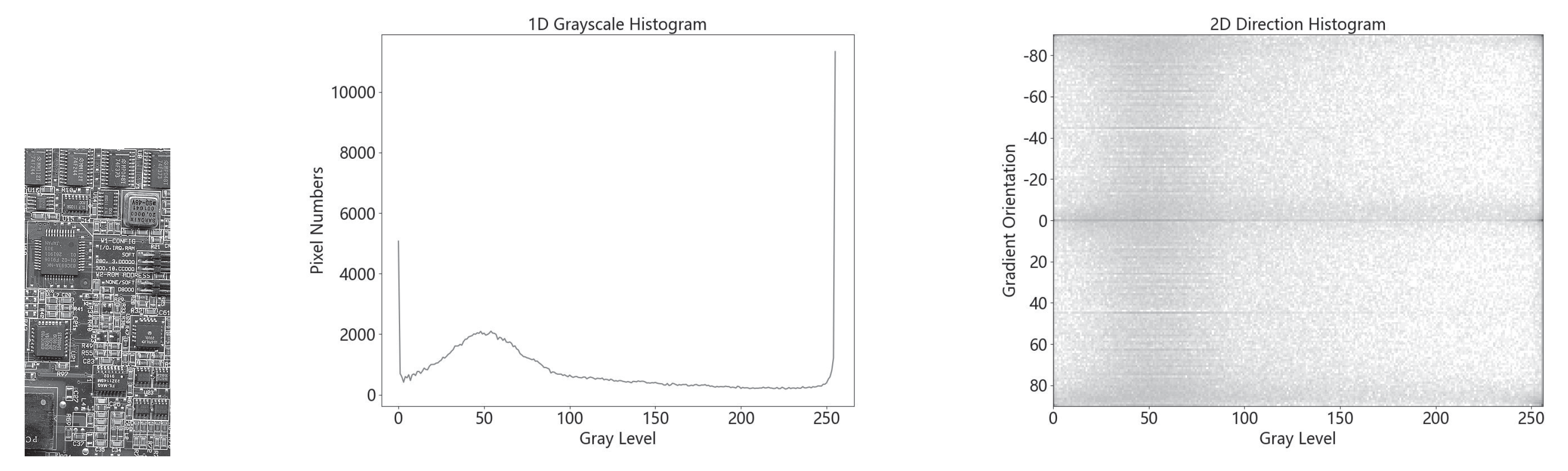
Figure 2.
Clustering results of the ’board’ image with the grayscale histogram of each: (a) pixels with k ranging from , (b) pixels with k ranging from , (c) pixels with k ranging from .
Figure 2.
Clustering results of the ’board’ image with the grayscale histogram of each: (a) pixels with k ranging from , (b) pixels with k ranging from , (c) pixels with k ranging from .
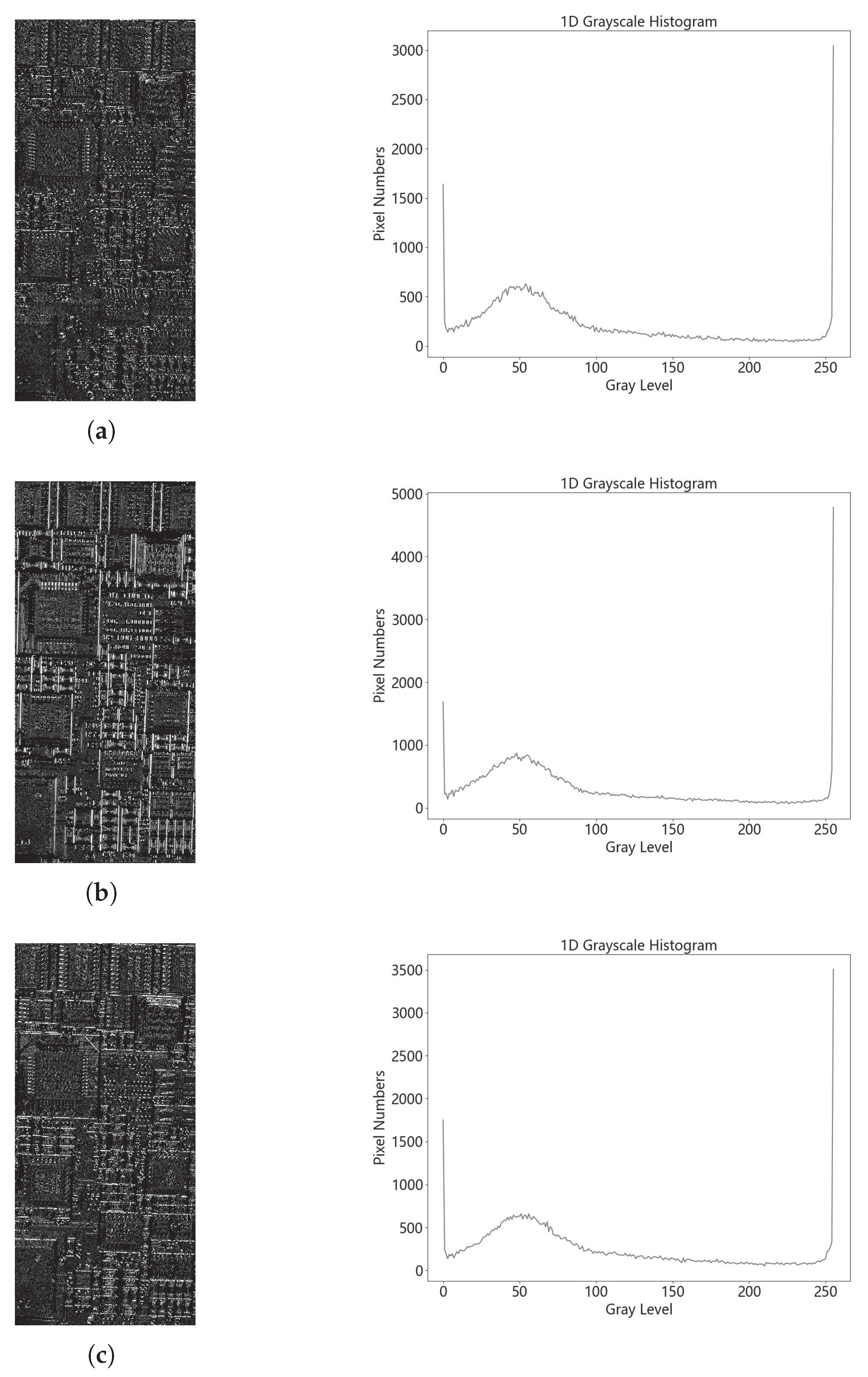
Figure 3.
The overall local thresholding segmentation based on the 2-D gradient orientation histogram.
Figure 3.
The overall local thresholding segmentation based on the 2-D gradient orientation histogram.
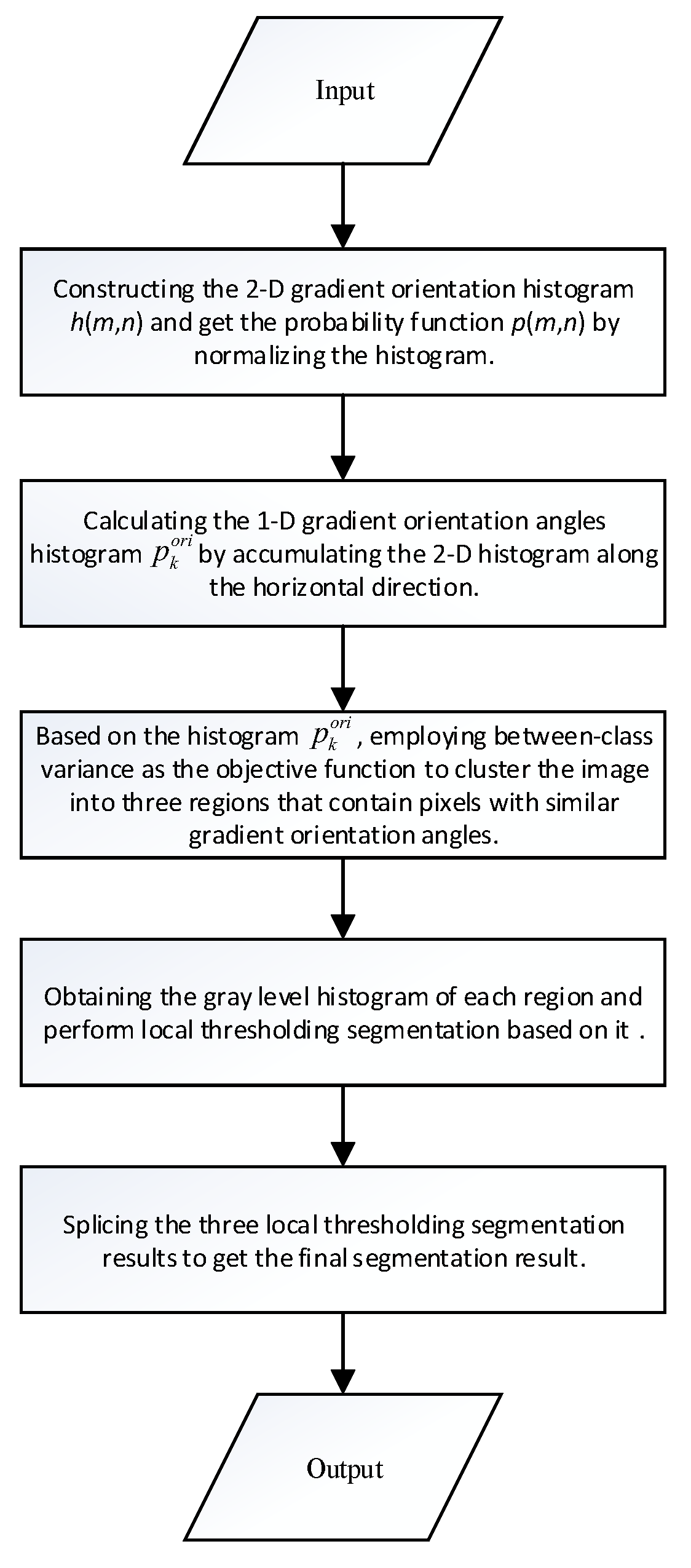
Figure 4.
Sample images from the MATLAB image library.
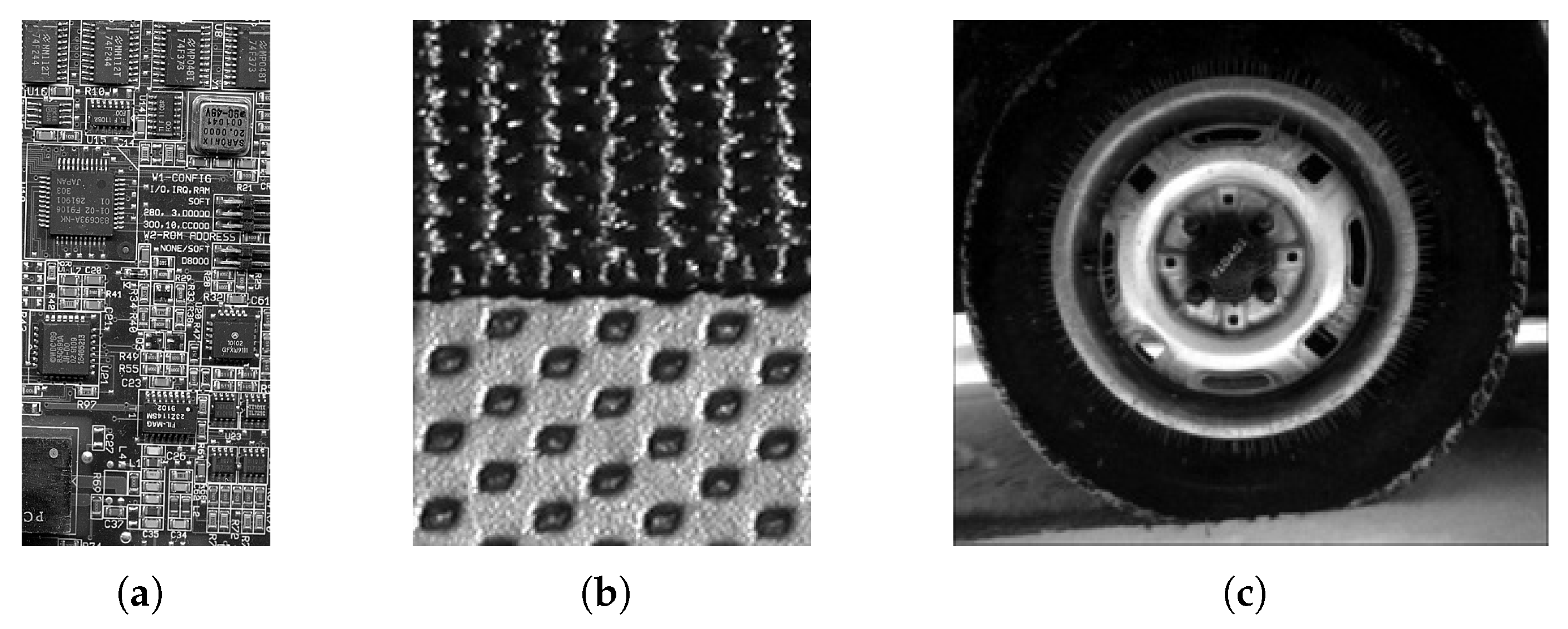
Figure 5.
Example images from 4 categories of the DTD image dataset.
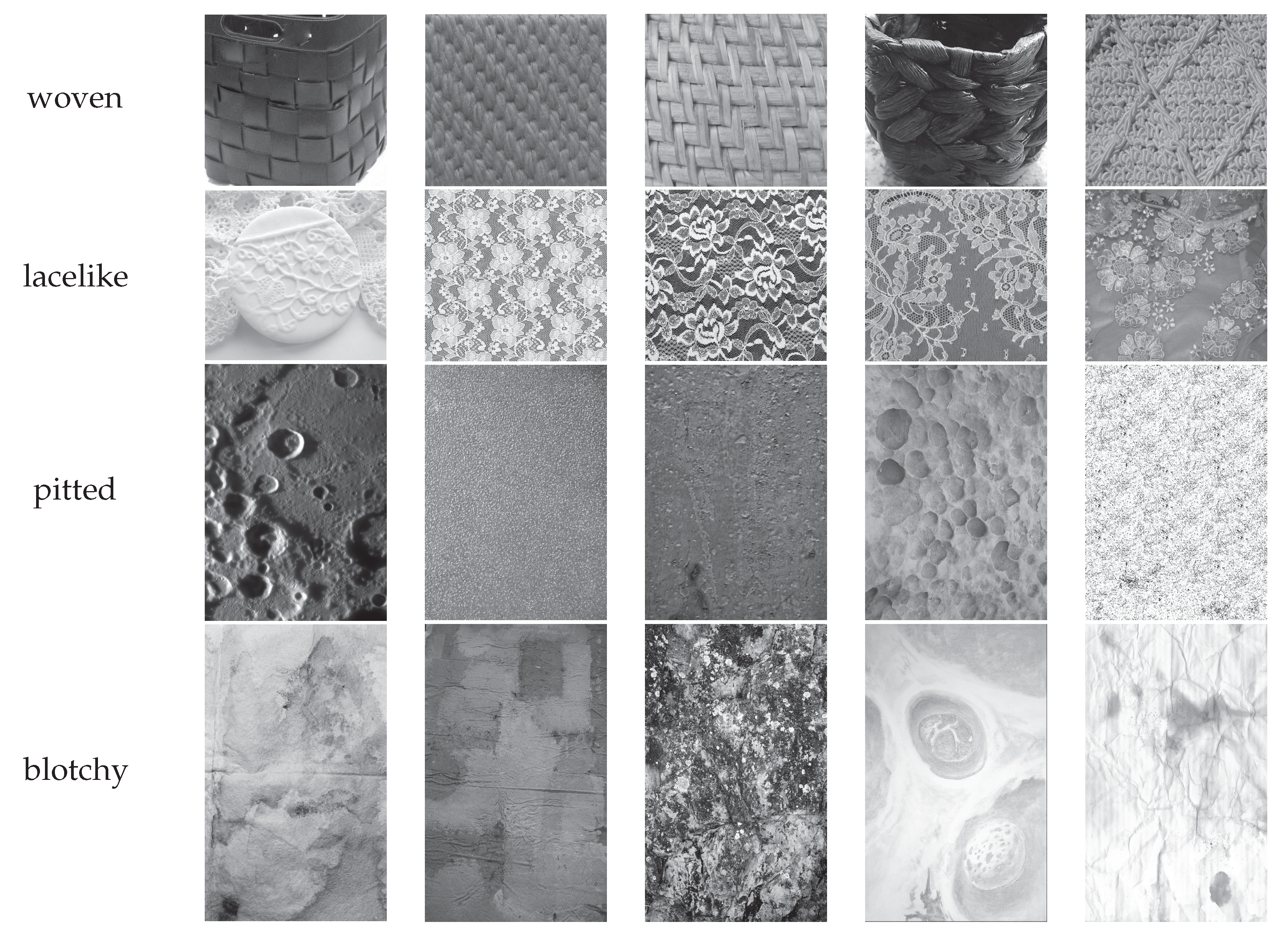
Figure 6.
The two-level thresholding results of the images from MATLAB library.
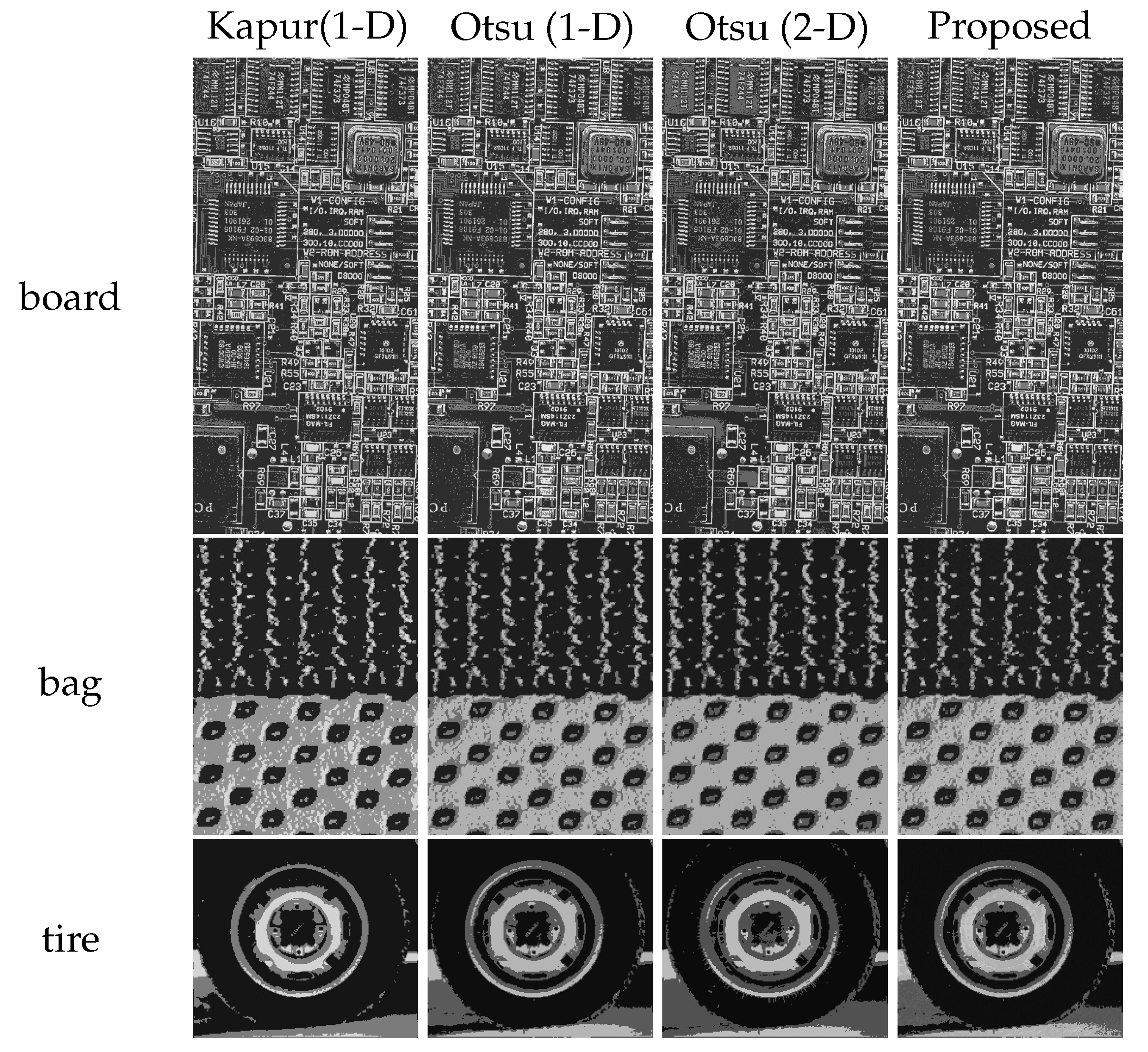
Figure 7.
The two-level thresholding results of the typical images from Figure 5 by using four algorithms.
Figure 7.
The two-level thresholding results of the typical images from Figure 5 by using four algorithms.


Table 1.
Comparisons of PSNR and FSIM values for multi-level thresholding on images from MATLAB image library based on 4 different algorithms.
Table 1.
Comparisons of PSNR and FSIM values for multi-level thresholding on images from MATLAB image library based on 4 different algorithms.
| Image | Thresholds | Kapur(1-D) | Otsu(1-D) | Otsu(2-D) | Proposed | ||||
|---|---|---|---|---|---|---|---|---|---|
| PSNR | FSIM | PSNR | FSIM | PSNR | FSIM | PSNR | FSIM | ||
| board | 2 | 19.8486 | 0.8417 | 20.5365 | 0.8594 | 20.1805 | 0.8603 | 21.7597 | 0.8654 |
| 3 | 22.0879 | 0.8925 | 23.0899 | 0.9254 | 20.9382 | 0.8703 | 23.0960 | 0.9304 | |
| 4 | 24.1754 | 0.9367 | 25.1001 | 0.9489 | 21.0960 | 0.8721 | 25.1076 | 0.9532 | |
| 5 | 25.9686 | 0.9539 | 26.7874 | 0.9635 | 21.0736 | 0.8719 | 26.7947 | 0.9665 | |
| bag | 2 | 21.0917 | 0.7064 | 21.7316 | 0.7291 | 21.6042 | 0.6936 | 21.7597 | 0.8037 |
| 3 | 23.9386 | 0.8154 | 24.1852 | 0.8388 | 22.1903 | 0.7096 | 24.2273 | 0.8677 | |
| 4 | 25.8303 | 0.8759 | 25.9751 | 0.8839 | 22.3528 | 0.7112 | 26.0317 | 0.9124 | |
| 5 | 27.2505 | 0.9106 | 27.5939 | 0.9154 | 22.3593 | 0.7113 | 27.6188 | 0.9226 | |
| tire | 2 | 20.9682 | 0.6295 | 22.0913 | 0.6762 | 21.0869 | 0.6406 | 22.1534 | 0.7417 |
| 3 | 24.7329 | 0.7427 | 24.7887 | 0.7439 | 24.2287 | 0.7270 | 24.8545 | 0.8013 | |
| 4 | 26.5611 | 0.7991 | 26.6432 | 0.8020 | 26.2494 | 0.7919 | 26.6680 | 0.8362 | |
| 5 | 27.4821 | 0.8282 | 28.2698 | 0.8414 | 26.6968 | 0.8075 | 28.3058 | 0.8686 | |
Table 2.
Computation time (seconds) of two-level thresholding using different algorithms.
| Kapur(1-D) | Otsu (1-D) | Otsu (2-D) | Proposed | |
|---|---|---|---|---|
| board | 0.32 | 0.27 | 147103.22 | 2.35 |
| bag | 0.32 | 0.27 | 135890.45 | 1.25 |
| tire | 0.32 | 0.27 | 142732.34 | 1.22 |
Table 3.
The optimal PSNR/FSIM distributions among four algorithms by using DTD image dataset at given number of thresholds.
Table 3.
The optimal PSNR/FSIM distributions among four algorithms by using DTD image dataset at given number of thresholds.
| Image | Thresholds | Kapur(1-D) | Otsu(1-D) | Otsu(2-D) | Proposed | ||||
|---|---|---|---|---|---|---|---|---|---|
| PSNR | FSIM | PSNR | FSIM | PSNR | FSIM | PSNR | FSIM | ||
| woven (81 images) |
2 | 0 | 5 | 2 | 8 | 0 | 9 | 81 | 60 |
| 3 | 0 | 16 | 0 | 4 | 0 | 0 | 81 | 61 | |
| 4 | 0 | 13 | 6 | 4 | 0 | 0 | 75 | 64 | |
| 5 | 0 | 13 | 1 | 4 | 0 | 0 | 80 | 64 | |
| lacelike (119 images) |
2 | 0 | 9 | 1 | 6 | 0 | 7 | 119 | 97 |
| 3 | 0 | 9 | 1 | 6 | 0 | 0 | 118 | 104 | |
| 4 | 0 | 12 | 16 | 9 | 0 | 0 | 103 | 98 | |
| 5 | 0 | 8 | 1 | 11 | 0 | 0 | 118 | 100 | |
| pitted (107 images) |
2 | 0 | 13 | 10 | 13 | 0 | 5 | 104 | 83 |
| 3 | 0 | 14 | 5 | 10 | 0 | 0 | 103 | 84 | |
| 4 | 0 | 15 | 6 | 20 | 0 | 0 | 105 | 76 | |
| 5 | 0 | 13 | 12 | 13 | 0 | 0 | 99 | 85 | |
| blotchy (119 images) |
2 | 0 | 7 | 15 | 11 | 2 | 4 | 113 | 105 |
| 3 | 0 | 8 | 13 | 13 | 0 | 1 | 112 | 103 | |
| 4 | 0 | 9 | 8 | 10 | 0 | 1 | 115 | 101 | |
| 5 | 0 | 8 | 14 | 11 | 0 | 0 | 109 | 103 | |
Disclaimer/Publisher’s Note: The statements, opinions and data contained in all publications are solely those of the individual author(s) and contributor(s) and not of MDPI and/or the editor(s). MDPI and/or the editor(s) disclaim responsibility for any injury to people or property resulting from any ideas, methods, instructions or products referred to in the content. |
© 2025 by the authors. Licensee MDPI, Basel, Switzerland. This article is an open access article distributed under the terms and conditions of the Creative Commons Attribution (CC BY) license (http://creativecommons.org/licenses/by/4.0/).
Copyright: This open access article is published under a Creative Commons CC BY 4.0 license, which permit the free download, distribution, and reuse, provided that the author and preprint are cited in any reuse.


