Submitted:
06 January 2026
Posted:
06 January 2026
Read the latest preprint version here
Abstract
This tutorial presents a coherent overview of reinforcement learning (RL), tracing its evolution from theoretical foundations to advanced deep learning algorithms. We begin with the mathematical formalization of sequential decision-making via Markov Decision Processes (MDPs). Central to RL theory is the Bellman equation for policy evaluation and its extension, the Bellman optimality equation, which provides the fundamental condition for optimal behavior. The journey from these equations to practical algorithms is explored, starting with model-based dynamic programming and progressing to model-free temporal-difference learning. We highlight Q-learning as a pivotal model-free algorithm that directly implements the Bellman optimality equation through sampling. To handle high-dimensional state spaces, the paradigm shifts to function approximation and deep reinforcement learning, exemplified by Deep Q-Networks (DQN). A significant challenge arises in continuous action spaces, addressed by actor-critic methods. We examine the Deep Deterministic Policy Gradient (DDPG) algorithm in detail, explaining how it adapts the principles of optimality to continuous control by maintaining separate actor and critic networks. The tutorial concludes with a unified perspective, framing RL's development as a logical progression from defining optimality conditions to developing scalable solution algorithms, and briefly surveys subsequent improvements and future directions, all underpinned by the enduring framework of the Bellman equations.
Keywords:
reinforcement learning
; tutorial
1. Introduction: How Do Machines Learn to Make Decisions?
Imagine teaching a robot to walk—you cannot specify the movement of every muscle in detail, but you can tell it “you’ll get a reward for walking well, and lose points for falling.” Through repeated attempts, the robot gradually figures out a stable walking method. This is the core idea of Reinforcement Learning (RL): an agent learns an optimal decision-making policy through interaction with the environment and trial-and-error.
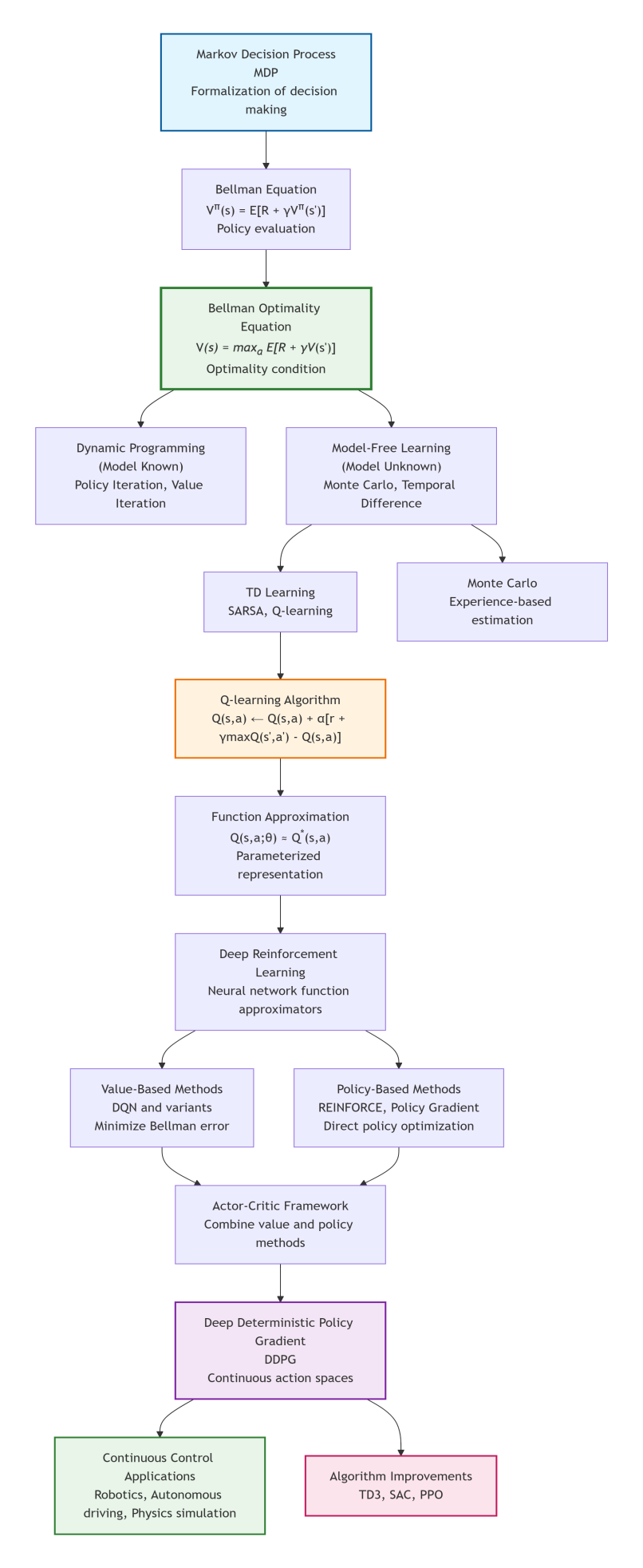
Reinforcement learning has made groundbreaking progress over the past decade, from AlphaGo defeating human Go champions to agents surpassing humans in complex games. Behind these achievements lies a series of sophisticated mathematical frameworks and algorithmic advancements. This tutorial guides you from the most fundamental MDP, step by step, to explore its core equations and algorithm evolution, up to understanding advanced algorithms like the DDPG, unveiling the mystery behind intelligent decision-making systems. The logistic structure of the tutorial is illustrated in Figure 1.
2. The Mathematical Foundation of Decision-Making—Markov Decision Process (MDP)
2.1. What Is the Markov Property?
The Markov Property is the core assumption of reinforcement learning: the future state depends only on the current state and not on past states. Mathematically:
This “memoryless” property greatly simplifies the modeling of decision problems.
2.2. The Five Elements of an MDP
A standard MDP consists of five key elements:
1) State Space (): The set of all possible situations of the environment.
2) Action Space (): The set of operations the agent can perform.
3) Transition Probability (): The probability distribution of state transitions after taking an action.
4) Reward Function (): The environment’s immediate feedback for a state-action 1) pair.
5) Discount Factor (γ): Measures the present value of future rewards (0 ≤ γ ≤ 1).
Remarks: The discount factor is similar to the concept of “present value” in economics—100 $ tomorrow is worth less than 100 $ today, and the agent also values immediate rewards more.
2.3. Policy and Return
A policy π is the agent’s decision rule, specifying what action to take in each state. The agent’s goal is to maximize the cumulative discounted return:
From Policy Evaluation to Optimal Policy—The Evolution of the Bellman Equation
3.1. State-Value Function and Action-Value Function
To evaluate the quality of a policy, RL introduces two core concepts:
1) State-value function : The expected return starting from state s and following policy π.
Action-value function : The expected return after taking action a in state s and thereafter following policy π.
3.2. The Bellman Equation: The Cornerstone of Policy Evaluation
The value functions satisfy an important recursive relationship—the Bellman Equation:
This equation reveals a profound insight: the value of the current state equals the immediate reward plus the discounted value of the successor state.
Logical Progression: The Bellman equation allows us to evaluate the quality of any given policy π, but it does not tell us how to find a better policy.
3.3. The Bellman Optimality Equation: The Beacon for Finding the Optimal Policy
The ultimate goal of RL is to find the optimal policy . This leads to one of the most central equations in RL theory: the Bellman Optimality Equation.
1) Optimality equation for the state-value function:
Optimality equation for the action-value function:
Remarks: The Bellman optimality equation no longer depends on a specific policy π, but directly defines the self-consistent condition that the optimal value functions must satisfy. It tells us: the optimal state value equals the value corresponding to the action that yields the maximum expected return; the optimal action value equals the immediate reward plus the maximum optimal action value of the successor state.
Real-world Analogy: Imagine finding the shortest path between cities. The Bellman equation tells you “how long it will take to reach the destination along the current route”; the Bellman optimality equation tells you “the shortest possible time from the current location to the destination, and which direction to go next.”
Logical Progression: From the Bellman equation to the Bellman optimality equation, we complete the conceptual leap from policy evaluation (analyzing a given policy) to policy optimization (finding the optimal policy). This equation is the theoretical foundation for all subsequent optimal control algorithms.
3.4. Dynamic Programming: Model-Based Solution Methods
When the environment’s dynamics model (P and R) are known, we can solve the Bellman optimality equation using dynamic programming methods:
Policy Iteration: Alternates between policy evaluation (solving the Bellman equation) and policy improvement.
Value Iteration: Directly iterates the Bellman optimality equation:
Logical Connection: The value iteration algorithm essentially repeatedly applies the Bellman optimality equation until the value function converges. This verifies that the Bellman optimality equation is not only descriptive but also constructive—it directly provides a solution algorithm.
4. Model-Free Learning—From Theory to Practice
4.1. Monte Carlo and Temporal Difference Learning
In real-world problems, the environment model is often unknown. Two model-free learning methods emerged:
1) Monte Carlo Methods: Estimate the value function using returns from complete trajectories.
Temporal Difference (TD) Learning: Combines ideas from Monte Carlo and dynamic planning, using estimated values for updates.
Where the TD error measures the discrepancy between prediction and actual outcome.
4.2. Q-Learning: A Practical Breakthrough from the Bellman Optimality Equation
Q-learning is a milestone algorithm in RL history. Its update rule derives directly from the Bellman optimality equation:
Remarks: Comparing the Q-learning update formula with the Bellman optimality equation, you’ll find that Q-learning is approximately solving the optimal equation through sampling. corresponds to in the optimal equation, and the entire update moves towards the optimal Q-value.
Key Feature: Off-policy learning—the agent learns the optimal action-value function to find the optimal policy, while potentially exploring other behaviors. This allows it to directly estimate the optimal Q-function without depending on the currently executed policy.
4.3. Function Approximation: Coping with High-Dimensional State Spaces
When the state space is huge or continuous, tabular methods become infeasible. Function approximation uses parameterized functions (e.g., neural networks) to represent value functions or policies:
where θ are learnable parameters. This paves the way for combining deep learning with reinforcement learning.
5. The Rise of Deep Reinforcement Learning
5.1. The Breakthrough of Deep Q-Networks (DQN)
Proposed by DeepMind in 2015, DQN achieved human-level performance on Atari games. Its main innovations include:
1) Experience Replay: Stores transition samples (s,a,r,s’) and randomly samples from them to break data correlations.
2) Target Network: Uses a separate target network to compute the TD target, stabilizing the learning process.
3) End-to-End Learning: Learns control policies directly from raw pixel input.
The DQN loss function essentially minimizes the error of the Bellman optimality equation:
where are the target network parameters.
Logical Unification: DQN can be viewed as a practical implementation that approximates the Q-function with a deep neural network and solves the Bellman optimality equation using stochastic gradient descent.
5.2. Policy Gradient: Directly Optimizing the Policy
Unlike value-based methods, policy gradient methods directly parameterize the policy π(a|s;θ) and optimize the expected return. The fundamental theorem is:
Core idea: Increase the probability of actions that lead to high returns and decrease the probability of actions that lead to low returns.
6. The Deep Deterministic Policy Gradient (DDPG) Algorithm
6.1. The Challenge of Continuous Action Spaces
Many practical problems (e.g., robot control, autonomous driving) require decision-making in continuous action spaces. Discrete-action methods like DQN face the curse of dimensionality—if each dimension has possible values, a d-dimensional action space has possible actions. More importantly, the ) operation in DQN becomes computationally intractable in continuous spaces.
6.2. The Core Idea of DDPG
The Deep Deterministic Policy Gradient is an actor-critic algorithm designed for continuous control, cleverly avoiding the maximization problem:
1) Deterministic Policy: directly outputs a deterministic action.
2) Actor-Critic Architecture:
Actor Network (Policy Network):, responsible for selecting actions.
Critic Network (Value Function Network):, evaluates the quality of actions.
3) Soft Update Mechanism: Target network parameters slowly track the online network parameters.
6.3. The Connection Between DDPG and the Bellman Optimality Equation
DDPG’s update rules embody the adaptation of Bellman optimality ideas to continuous spaces:
1) Critic Update (based on the continuous form of the Bellman optimality equation):
Note that the target policy network μ’ replaces the max operation here, as the deterministic policy directly gives the optimal action selection.
2) Actor Update(improving the policy along the gradient of the Q-function):
The actor network is trained to output actions that maximize the Q-value, which is essentially the “policy improvement” step in continuous action spaces.
6.4. DDPG Algorithm
The Pseudocode is listed as follows:
| Initialize actor network and critic network Initialize corresponding target networks μ’ and Q’ Initialize experience replay buffer R for each time step do Select action a = + exploration noise Execute a, observe reward r and new state s’ Store transition (s,a,r,s’) in R Randomly sample a minibatch from R # Update critic (based on modified Bellman optimality equation) # Update actor (approximate policy improvement) |
Theoretical Connection: DDPG can be seen as an approximate method for solving the Bellman optimality equation in continuous spaces. The critic learns the optimal Q-function, the actor learns the corresponding optimal policy, and they are optimized alternately, similar to policy iteration in dynamic programming.
6.5. Advantages and Challenges of DDPG
Advantages:
1) Efficiently handles continuous action spaces, avoiding the curse of dimensionality.
2) Relatively high sample efficiency.
3) Can learn deterministic policies, suitable for tasks requiring precise control.
Challenges:
1) Sensitive to hyperparameters.
2) Exploration efficiency issues (requires carefully designed exploration noise).
3) May converge to local optima.
7. Frontier Developments and a Unified Theoretical Perspective
7.1. Subsequent Improved Algorithms
Following DDPG, researchers proposed various improved algorithms, all revolving around the core of solving the Bellman optimality equation more stably:
1) TD3 (Twin Delayed Deep Deterministic Policy Gradient): Addresses overestimation via double Q-learning, a correction for errors in the max operator of the Bellman optimality equation.
2) SAC(Soft Actor-Critic): Introduces a maximum entropy framework, modifying the Bellman equation to encourage exploration.
3) PPO(Proximal Policy Optimization): Stabilizes training by constraining policy updates, ensuring monotonic policy improvement.
7.2. A Unified Theoretical Perspective on Reinforcement Learning
From Markov Decision Processes to the Deep Deterministic Policy Gradient, the development of reinforcement learning presents a clear logical thread. Table 1 shows this complete framework of theoretical evolution and algorithmic development.
Key Turning Points in Logical Evolution:
1) From Evaluation to Optimization: Bellman Equation → Bellman Optimality Equation.
2) From Known to Unknown: Dynamic Programming (model known) → Model-Free Learning.
3) From Discrete to Continuous: Tabular methods → Function Approximation → Deep Neural Networks.
4) From Value Function to Policy: Value-based methods → Policy Gradient → Actor-Critic.
5) From Theory to Practice: Theoretical equations → Practical algorithms → Engineering implementation.
7.3. Future Directions
1) Theoretical Deepening: Deeper understanding of the generalization capabilities and convergence properties of deep reinforcement learning.
2) Algorithmic Efficiency: Improving sample efficiency, reducing the need for environment interaction.
3) Safety and Reliability: Ensuring safety during exploration.
4) Multi-Task Learning: Enabling transfer of knowledge and skills.
8. Conclusion: The Science of Intelligent Decision-Making Within a Unified Framework
From the mathematical formalization of Markov Decision Processes, to the establishment of the Bellman equation, and further to the theoretical breakthrough of the Bellman optimality equation, reinforcement learning has built a complete theoretical system for decision-making. Q-learning transformed the optimality equation into a practical algorithm, deep neural networks solved the problem of high-dimensional representation, and algorithms like DDPG extended it to the domain of continuous control.
This development history reveals a profound scientific methodology: from clear problem definition (MDP), to establishing optimality conditions (Bellman optimality equation), to developing practical solution algorithms (from dynamic programming to deep reinforcement learning). Each layer of progress is built upon a solid theoretical foundation while simultaneously pushing the theory further.
Today, reinforcement learning continues to develop rapidly, but its core still revolves around the fundamental problem of how to make optimal decisions in uncertain environments. The Bellman optimality equation, as the North Star of this field, continues to guide the development direction of new algorithms. With increasing computational power and theoretical refinement, we have reason to believe that intelligent systems based on these principles will play key roles in more and more complex decision-making tasks, ultimately helping us solve some of the most challenging problems facing society.
As Richard Bellman himself might have foreseen, the equation he proposed not only became the cornerstone of reinforcement learning but also opened a new era of enabling machines to learn autonomous decision-making. The path of exploration from theoretical equations to practical algorithms continues, and each step brings us closer to truly intelligent machine decision systems.
References
- Bellman, R. Dynamic Programming; Princeton University Press, 1957. [Google Scholar]
- Sutton, R. S.; Barto, A. G. Reinforcement Learning: An Introduction, 2nd ed.; MIT Press, 2018. [Google Scholar]
- Watkins, C. J. C. H.; Dayan, P. Q-learning. Machine Learning 1992, 8(3-4), 279–292. [Google Scholar] [CrossRef]
- Mnih, V.; Kavukcuoglu, K.; Silver, D.; Rusu, A. A.; Veness, J.; Bellemare, M. G.; Graves, A.; Riedmiller, M.; Fidjeland, A. K.; Ostrovski, G.; Petersen, S.; Beattie, C.; Sadik, A.; Antonoglou, I.; King, H.; Kumaran, D.; Wierstra, D.; Legg, S.; Hassabis, D. Human-level control through deep reinforcement learning. Nature 2015, 518(7540), 529–533. [Google Scholar] [CrossRef]
- Lillicrap, T. P.; Hunt, J. J.; Pritzel, A.; Heess, N.; Erez, T.; Tassa, Y.; Silver, D.; Wierstra, D. Continuous control with deep reinforcement learning. International Conference on Learning Representations (ICLR) 2016. [Google Scholar]
- Fujimoto, S.; van Hoof, H.; Meger, D. Addressing function approximation error in actor-critic methods. International Conference on Machine Learning (ICML) 2018. [Google Scholar]
- Haarnoja, T.; Zhou, A.; Abbeel, P.; Levine, S. Soft actor-critic: Off-policy maximum entropy deep reinforcement learning with a stochastic actor. International Conference on Machine Learning (ICML) 2018. [Google Scholar]
- Schulman, J.; Wolski, F.; Dhariwal, P.; Radford, A.; Klimov, O. Proximal policy optimization algorithms. arXiv 2017, arXiv:1707.06347. [Google Scholar] [CrossRef]
- Silver, D.; Lever, G.; Heess, N.; Degris, T.; Wierstra, D.; Riedmiller, M. Deterministic policy gradient algorithms. International Conference on Machine Learning (ICML) 2014. [Google Scholar]
- Arulkumaran, K.; Deisenroth, M. P.; Brundage, M.; Bharath, A. A. A brief survey of deep reinforcement learning. IEEE Signal Processing Magazine 2017, 34(6), 26–38. [Google Scholar] [CrossRef]
Figure 1.
Logistic structure of the tutorial.

Table 1.
Correspondence between Theoretical Foundations and Algorithm Evolution.
| Theoretical Stage | Core Concept | Mathematical Expression | Representat-ive Algorithms | Applicable Scenarios |
|---|---|---|---|---|
| Problem Definition | Markov Decision Process | - | Decision problem formulation | |
| Policy Evaluation | Bellman Equation | Policy evaluation algorithms | Analyzing a given policy | |
| Optimal Condition | Bellman Optimality Equation | Theoretical benchmark | Defining optimal policy standard | |
| Model-Based Solution | Dynamic Programming | Value iteration, Policy iteration | Environments with known model | |
| Model-Free Learning | Temporal Difference Learning |
|
SARSA, Q-learning | Environments with unknown model |
| High-Dimensional Extension | Function Approximation | Linear function approximation | Large state spaces | |
| Deep Integration | Deep Q-Learning |
|
DQN and its variants | High-dimensional inputs like images |
| Policy Optimization | Policy Gradient | REINFORCE | Direct policy optimization | |
| Integrated Methods | Actor-Critic | actor: |
A3C, DDPG | Continuous action spaces |
| Continuous Control | Deterministic Policy Gradient | DDPG, TD3, SAC | Robot control, etc. |
Disclaimer/Publisher’s Note: The statements, opinions and data contained in all publications are solely those of the individual author(s) and contributor(s) and not of MDPI and/or the editor(s). MDPI and/or the editor(s) disclaim responsibility for any injury to people or property resulting from any ideas, methods, instructions or products referred to in the content. |
© 2026 by the author. Licensee MDPI, Basel, Switzerland. This article is an open access article distributed under the terms and conditions of the Creative Commons Attribution (CC BY) license.
Copyright: This open access article is published under a Creative Commons CC BY 4.0 license, which permit the free download, distribution, and reuse, provided that the author and preprint are cited in any reuse.


