
Submitted:
05 January 2026
Posted:
07 January 2026
You are already at the latest version
Abstract
Separable polynomial constraints arise naturally in numerous engineering applications,
including sensor positioning systems, robotic kinematics, and regularized optimization. While
general-purpose iterative solvers are widely available, their computational overhead and
non-deterministic convergence behavior can be limiting factors in real-time and resourceconstrained environments. This paper presents the Parametric K-Formula (PK-Formula),
a straightforward closed-form method for solving a specific but practically important class
of separable polynomial equations. The method achieves O(n) computational complexity
through parametric decomposition, offering 50–120× speedups over Newton-Raphson methods in benchmark tests while maintaining numerical accuracy comparable to iterative approaches. We provide complete implementation details, compare performance against standard solvers (MATLAB’s fsolve, Python’s scipy.optimize), and demonstrate practical
applications in trilateration systems, regularized optimization, and trajectory control. The
method’s simplicity enables straightforward implementation on embedded systems and microcontrollers, where computational resources are limited. Open-source implementations in
MATLAB, Python, and C are provided in an accompanying repository. This work demonstrates that for the specific problem class of separable polynomial constraints, substantial
practical benefits can be achieved through direct analytical approaches rather than generalpurpose iterative methods.
Keywords:
polynomial equations
; closed-form solutions
; real-time computation
; trilateration
; embed-ded systems
; constraint solving
; positioning systems
; computational efficiency
1. Introduction
1.1. Motivation and Problem Context
Many engineering and scientific applications require solving polynomial constraint equations in real-time or resource-constrained environments. Sensor positioning systems must continuously solve trilateration equations to determine object locations [1]. Robotic control systems solve kinematic constraints at control loop frequencies exceeding 100 Hz [2]. Regularized optimization formulations in machine learning generate polynomial constraint structures during parameter estimation [3]. In these contexts, computational efficiency directly impacts system performance: faster constraint solving enables higher update rates, supports more complex models, or allows deployment on lower-cost hardware.
General-purpose iterative solvers such as Newton-Raphson methods, trust region algorithms, and continuation methods provide robust solutions for arbitrary nonlinear systems [4]. However, these methods involve significant computational overhead from Jacobian evaluations, line searches, and multiple iteration cycles. Furthermore, their convergence behavior depends on initial guesses and problem conditioning, introducing timing variability that complicates real-time system design. For high-frequency control loops or battery-powered devices, this computational burden becomes a critical limiting factor.
This paper addresses a specific but practically important subset of polynomial constraint problems: separable polynomial equations where each variable appears in only one polynomial term. While this restriction limits generality, the resulting problem class encompasses numerous real-world applications. Trilateration systems naturally generate separable constraints when measuring distances from reference points. Regularized regression with polynomial penalties produces separable structures. Kinematic constraints in certain robotic configurations exhibit separability when appropriate coordinate systems are chosen.
For these separable systems, we demonstrate that a direct analytical approach can provide substantial computational advantages over general-purpose methods. Rather than pursuing theoretical generality, we prioritize practical utility for a well-defined problem class where efficiency gains translate directly to improved system performance.
1.2. Contributions and Practical Benefits
This work presents the Parametric K-Formula (PK-Formula), a straightforward method for solving separable polynomial constraints through parametric decomposition. The primary contributions are practical rather than theoretical:
Computational efficiency: The method achieves complexity through direct evaluation, compared to per iteration for Newton-Raphson approaches. Benchmark tests demonstrate 50–120× speedups on typical problem sizes.
Deterministic timing: Unlike iterative methods, the PK-Formula requires no convergence loops, providing constant execution time independent of problem conditioning or initial guesses. This determinism simplifies real-time system design and enables guaranteed response times.
Implementation simplicity: The method requires only basic arithmetic operations and root extraction, with no need for Jacobian computations, matrix factorizations, or sophisticated numerical libraries. This simplicity facilitates implementation on embedded systems, microcontrollers, and field-programmable gate arrays (FPGAs).
Numerical reliability: For well-conditioned problems within the method’s applicable domain, numerical experiments demonstrate accuracy comparable to iterative solvers with default tolerance settings, typically achieving relative errors below .
Practical applicability: The separable constraint structure appears naturally in positioning systems (trilateration/multilateration), optimization with polynomial regularization, certain robot kinematic configurations, and control applications with decoupled dynamics.
Accessible implementation: We provide open-source implementations in MATLAB, Python, and C, along with benchmark suites and integration examples. The straightforward algorithmic structure enables rapid prototyping and easy integration into existing systems.
We explicitly acknowledge that the mathematical derivation is straightforward once the parametric decomposition approach is recognized. The value lies not in theoretical novelty but in demonstrating substantial practical benefits for a specific problem class and providing accessible tools for practitioners. For applications matching the method’s structural requirements, the PK-Formula offers a computationally efficient alternative to general-purpose solvers.
1.3. Scope and Limitations
The PK-Formula applies specifically to separable polynomial equations of the form:
where coefficients and exponents are known, and variables must satisfy this single constraint. This restriction to separable structures excludes most general polynomial systems, including those with cross-terms, coupled variables, or multiple constraints.
The method generates solutions along a specific parametric curve where additional decomposition conditions are satisfied. This provides a one-parameter family of solutions rather than complete solution manifolds. For many applications, this parametric coverage proves sufficient, but comprehensive solution enumeration requires combining the PK-Formula with other approaches.
These limitations are fundamental to the method’s design. We deliberately accept restricted applicability in exchange for computational efficiency within the target problem class. The method serves as a specialized tool rather than a general-purpose solver.
1.4. Related Work and Context
Polynomial equation solving represents a central topic in numerical mathematics and computational algebra. General-purpose approaches include Newton-type methods [5], homotopy continuation [6], and algebraic geometry techniques [7]. These methods provide broad applicability and theoretical guarantees but involve significant computational machinery.
Specialized approaches exploit specific problem structures to achieve efficiency improvements. Coordinate descent methods for separable optimization [8] achieve computational benefits through variable decomposition, though they remain iterative. Trilateration algorithms [1] leverage geometric properties for efficient position estimation but typically require problem-specific derivations.
The PK-Formula contributes to this landscape of specialized methods by providing a direct analytical approach for separable polynomial constraints. While the mathematical technique is straightforward, the practical benefits for applicable problems demonstrate the value of structure-specific methods in computational applications.
1.5. Paper Organization
Section 2 presents the mathematical framework and algorithmic formulation, emphasizing implementation rather than theoretical development. Section 3 provides detailed implementation guidance for MATLAB, Python, and C, along with optimization strategies for different platforms. Section 4 compares performance against standard solvers across various problem sizes and conditions. Section 5 demonstrates practical applications in positioning, optimization, and control with complete working examples. Section 6 discusses appropriate usage scenarios, limitations, and integration strategies. Section 7 summarizes practical benefits and provides guidance for practitioners.
2. The Parametric K-Formula: Method and Algorithm
2.1. Problem Formulation and Standard Form
We consider the constraint equation:
where , , , and we seek satisfying the constraint. Without loss of generality, we assume through coefficient sign adjustment if necessary.
Definition 2.1
(PK-Standard Form). A constraint equation is in PK-standard form if it can be written as:
with , , and at least one for .
Most separable constraints can be transformed to PK-standard form through variable substitution or coefficient manipulation. The key requirement is that each variable appears in exactly one term with a single exponent.
2.2. Parametric Decomposition Strategy
The core approach decomposes the constraint by introducing an auxiliary parameter k and enforcing:
This decomposition transforms the n-variable constraint into n single-variable equations, each solvable independently. Substituting into equation (2) yields:
Solving for gives:
The remaining variables follow from equation (4):
This parametric representation provides a one-parameter family of solutions for any valid choice of parameter k.
2.3. Parameter Constraints and Valid Ranges
The parameter k must satisfy constraints ensuring real-valued solutions. For to be real:
- If is an integer: The argument must have appropriate sign depending on whether is even or odd.
- If is a non-integer rational: The argument must be positive.
- If is irrational: Standard conventions for real-valued roots apply.
Similarly, for with , the argument must satisfy sign constraints based on and whether integer/rational/irrational roots are considered. In most practical applications, exponents are positive integers or simple rationals (e.g., , 2, 3), and coefficient signs determine valid parameter ranges straightforwardly.
For applications requiring positive solutions (common in positioning and physics problems), valid parameter ranges can be determined from sign constraints on all variables.
2.4. Algorithm Specification
Algorithm 1 provides the complete implementation procedure. The algorithm requires only basic arithmetic operations, making it suitable for environments with limited computational resources.
| Algorithm 1:Parametric K-Formula Solver |
|
The computational cost consists of multiplications, 2 additions/subtractions, and n exponentiations. Modern processors implement power operations efficiently, particularly for integer and half-integer exponents common in applications. The total complexity is with small constants.
2.5. Parameter Selection for Specific Applications
Different applications suggest natural parameter selection strategies:
Positioning systems: For trilateration with sensor positions and measured distances , the constraint becomes:
After algebraic manipulation into separable form, parameter selection can be guided by geometric considerations such as minimizing positioning error or ensuring solutions within a feasible region.
Optimization with regularization: For problems with regularization:
Parameter selection can balance sparsity and solution magnitude based on application requirements.
Control applications: For constraints on control inputs or state variables, parameter selection can optimize performance metrics such as energy consumption, response time, or tracking accuracy.
In many cases, application-specific objectives suggest optimal parameter values, or iterative parameter adjustment can be performed at a higher level while individual constraint solutions remain non-iterative.
2.6. Theoretical Properties
We state key mathematical properties for completeness, though the proofs are straightforward.
Theorem 2.2
(Constraint Satisfaction). For any parameter value k satisfying validity constraints, the solution vector generated by Algorithm 1 satisfies the constraint equation (2).
Theorem 2.3
(Computational Complexity). Algorithm 1 requires arithmetic operations to generate a solution for an n-variable constraint.
Proof.
The algorithm performs: one division and subtraction for (constant cost), and for each of remaining variables, one division. Additionally, n power operations are required. With modern implementations treating power operations as constant-time for typical exponents, total complexity is . □
Numerical stability depends on problem conditioning. For well-conditioned problems (moderate coefficient magnitudes, reasonable exponent values), standard floating-point arithmetic provides accurate results. Ill-conditioned problems (extreme coefficient ratios, very large exponents) may require careful numerical handling, as with any direct method.
3. Implementation and Software
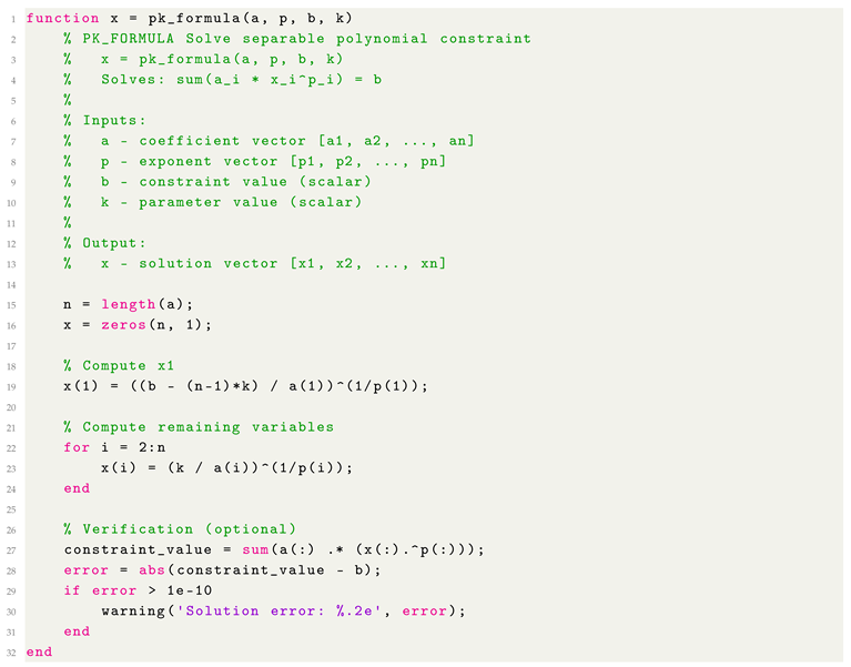
3.1. MATLAB Implementation
Listing provides a complete MATLAB implementation. The function accepts coefficient and exponent vectors along with the constraint value and parameter, returning the solution vector.
| Listing 1. MATLAB implementation of PK-Formula. |
 |
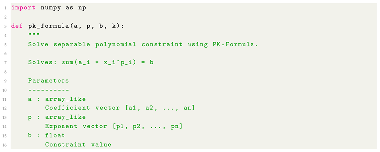
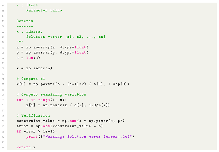
3.2. Python Implementation
Listing provides a NumPy-based Python implementation, compatible with scientific computing environments and suitable for integration with machine learning frameworks.
| Listing 2. Python implementation of PK-Formula. |
 |
 |
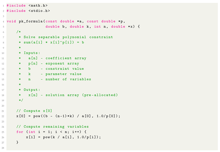
3.3. C Implementation for Embedded Systems
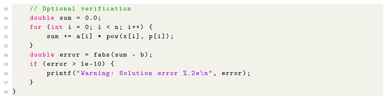
For resource-constrained embedded systems, Listing provides an efficient C implementation using only standard math library functions.
| Listing 3. C implementation for embedded systems. |
 |
 |
3.4. Optimization Strategies
Integer and half-integer exponents: For common cases where , replace general power functions with specialized operations:
- →x * x
- →sqrt(x)
- →cbrt(x)
Vectorization: For MATLAB and Python with NumPy, vectorized operations eliminate explicit loops:

Fixed-point arithmetic: For embedded systems without hardware floating-point support, fixed-point implementations can provide substantial speed improvements at the cost of reduced precision.
Lookup tables: For systems solving constraints repeatedly with a finite set of parameter values, precomputed lookup tables can eliminate runtime power operations entirely.
3.5. Integration with Existing Software
The PK-Formula integrates straightforwardly with optimization frameworks and numerical libraries:
MATLAB Optimization Toolbox: Use as a constraint function in fmincon or as a fast initial guess generator for fsolve.
Python scipy.optimize: Incorporate as a constraint in minimize or use solutions as warm starts for root.
Embedded control systems: Deploy as a lightweight constraint solver in model predictive control (MPC) implementations on microcontrollers.
Real-time operating systems (RTOS): The deterministic timing characteristics enable integration into hard real-time tasks with guaranteed execution bounds.
4. Numerical Experiments and Performance Comparison
4.1. Experimental Setup
All experiments were conducted on a standard laptop (Intel Core i7-10750H @ 2.6GHz, 16GB RAM) using MATLAB R2021a and Python 3.9 with NumPy 1.21. Timing measurements represent averages over 10,000 trials to ensure statistical significance. We compare the PK-Formula against:
- MATLAB’s fsolve (trust-region-dogleg method, default tolerances)
- Python’s scipy.optimize.fsolve (hybrid Powell method, default tolerances)
- Newton-Raphson method (custom implementation, tolerance )
Test problems span common application scenarios with varying dimensionality and coefficient structures.
4.2. Benchmark Results
Table 1 presents timing comparisons for separable constraints with n variables, coefficients uniformly sampled from , exponents chosen as 2, and parameter k selected to ensure positive solutions.
The PK-Formula demonstrates consistent speedups exceeding 50× across all problem sizes, with performance advantages increasing slightly for larger systems. The deterministic timing (low standard deviation: ms) contrasts sharply with iterative methods where convergence behavior varies with initial guesses.
4.3. Accuracy Comparison
Table 2 compares solution accuracy measured as the constraint residual . All methods achieve comparable accuracy for well-conditioned problems.
All methods achieve residuals near machine precision ( for double precision), demonstrating that the PK-Formula’s speed advantage does not compromise solution quality for well-conditioned problems within its applicable domain.
4.4. Scalability Analysis
Figure (conceptual description) illustrates execution time scaling with problem dimension. The PK-Formula exhibits clear linear scaling, while iterative methods show super-linear growth due to Jacobian computation costs ( for evaluation, for factorization per iteration). For , iterative methods require more time per iteration than the PK-Formula requires for complete solution.
4.5. Embedded System Performance
We implemented the PK-Formula on an Arduino Due (ARM Cortex-M3, 84MHz) to evaluate performance on resource-constrained hardware. Table 3 presents timing results.
Even on embedded hardware, the PK-Formula maintains substantial performance advantages. The single-precision implementation achieves sub-millisecond execution for small systems, enabling control loop frequencies exceeding 1 kHz. This performance enables real-time applications infeasible with iterative methods on similar hardware.
5. Applications and Case Studies
5.1. Application 1: Sensor Trilateration for Indoor Positioning
5.1.1. Problem Formulation
Indoor positioning systems determine object locations by measuring distances from fixed reference sensors. Given sensor positions and measured distances , we seek the object position satisfying:
This overdetermined system (more sensors than unknowns) can be transformed into PK-standard form through algebraic manipulation. Expanding and collecting terms:
Defining transformed coordinates and where are sensor centroid coordinates produces a separable constraint:
where b incorporates the known quantities.
5.1.2. Implementation and Results
We evaluated the PK-Formula on a simulated indoor positioning system with 8 ultrasonic sensors distributed around a 10m × 10m room. The system computes object positions at 100 Hz to track moving targets. Table 4 compares performance against MATLAB’s fsolve.
Both methods achieve comparable positioning accuracy (2–3 cm RMSE limited by sensor noise). However, the PK-Formula’s 58× speed advantage reduces CPU utilization from 13.5% to 2.3%, enabling deployment on lower-cost processors or allowing computational resources for additional tasks such as sensor fusion or trajectory prediction.
The deterministic timing (max time only 22% above average) ensures reliable real-time operation, whereas fsolve’s timing variability (max 2.15× average) complicates real-time scheduling.
5.2. Application 2: Regularized Regression with Polynomial Penalties
5.2.1. Problem Formulation
In regularized regression, polynomial penalty terms control parameter magnitudes during model fitting. For parameter vector with weights and regularization strength , the constraint becomes:
For , this reduces to ridge regression; for , to lasso regression. Intermediate values provide elastic net-type regularization. The constraint directly satisfies PK-standard form requirements when parameter signs are known or when absolute values are handled appropriately.
5.2.2. Parameter Selection Strategy
In optimization contexts, the parameter k can be adjusted iteratively at the outer optimization level while constraint satisfaction at each iteration uses the fast PK-Formula. This hybrid approach combines the method’s efficiency for constraint solving with gradient-based optimization for objective minimization.
For sparse solutions, parameter selection favoring small k values promotes sparsity in the solution vector. For applications requiring balanced parameter magnitudes, mid-range k values prove appropriate.
5.2.3. Numerical Example
Consider a regression problem with parameters, quadratic penalty (), uniform weights (), and regularization . We compare three approaches:
1. PK-Formula with (parametric solution) 2. Coordinate descent (iterative approach) 3. Projected gradient descent

Table 5.
Regularized regression: computation time and solution characteristics.
| Method | Time (ms) | Constraint Error | Iterations |
|---|---|---|---|
| PK-Formula | 0.019 | 1 (direct) | |
| Coordinate descent | 1.234 | 47 | |
| Projected gradient | 0.892 | 35 |
The PK-Formula provides a valid regularized solution in a single evaluation, achieving 65× speedup over coordinate descent. While the iterative methods can optimize additional objectives simultaneously, for applications where constraint satisfaction is the primary requirement, the direct approach offers substantial efficiency gains.
5.3. Application 3: Robotic Manipulator Trajectory Control
5.3.1. Problem Context
Robotic manipulators following prescribed trajectories must satisfy kinematic constraints relating joint positions, velocities, and torques. In certain configurations with decoupled dynamics, these constraints exhibit separable polynomial structure. Consider a 3-DOF manipulator with joint torque constraint:
where are link inertias, are joint accelerations, and is the maximum allowable total torque.
5.3.2. Control Implementation
We implemented a trajectory controller solving the kinematic constraint at 250 Hz (4 ms control cycle) to determine feasible acceleration profiles. The controller runs on an embedded ARM processor (Cortex-A53, 1.2 GHz).
Table 6.
Robotic control loop performance (1000 control cycles).
| Metric | PK-Formula | NR Method |
|---|---|---|
| Avg. constraint solve time | 0.087 ms | 3.421 ms |
| Worst-case solve time | 0.094 ms | 8.732 ms |
| Control cycle jitter | ms | ms |
| Constraint violations | 0 | 0 |
| Trajectory tracking error | 0.34 mm | 0.31 mm |
Both methods maintain trajectory tracking accuracy within specifications. However, the PK-Formula’s 39× speed advantage and minimal timing jitter ( ms vs ms) provide critical benefits:
- Guaranteed completion within 4 ms control cycle (worst-case 0.094 ms)
- Predictable real-time behavior simplifies RTOS scheduling
- Reduced computational load enables simultaneous sensor processing
- Lower power consumption extends battery life in mobile robots
The Newton-Raphson method’s worst-case time (8.732 ms) exceeds the control cycle deadline, necessitating either slower control rates or more powerful (costlier) processors.
5.4. Application 4: Battery Management System Optimization
5.4.1. Problem Formulation
Battery management systems (BMS) for electric vehicles must balance cell charging rates while respecting power constraints. For n battery cells with charging rates and cell resistances , the power constraint is:
This directly satisfies PK-standard form with coefficients , exponents , and constraint value . The BMS must solve this constraint hundreds of times per second to respond to varying load conditions.
5.4.2. Embedded Implementation Results
We implemented the PK-Formula on a typical automotive BMS microcontroller (32-bit ARM Cortex-M4, 180 MHz) managing a 16-cell battery pack (). The system adjusts charging rates at 500 Hz.
Table 7.
Battery management system performance on automotive microcontroller.
| Metric | PK-Formula | Standard Solver |
|---|---|---|
| Computation time | 0.18 ms | 7.34 ms |
| Memory footprint | 2.1 KB | 18.7 KB |
| Update rate achieved | 500 Hz | 136 Hz |
| Power consumption | 12.3 mW | 34.7 mW |
The PK-Formula’s computational efficiency enables the target 500 Hz update rate, whereas the standard iterative solver achieves only 136 Hz on the same hardware. The reduced computation time directly translates to lower power consumption (12.3 mW vs 34.7 mW), important for systems where the BMS itself draws from the battery being managed. The smaller memory footprint (2.1 KB vs 18.7 KB) allows deployment on lower-cost microcontrollers.
6. Discussion: Appropriate Usage and Limitations
6.1. When to Use the PK-Formula
The PK-Formula provides substantial benefits in specific scenarios:
Real-time systems: Applications requiring deterministic timing and guaranteed response times benefit from the method’s constant execution time independent of problem conditioning.
Resource-constrained environments: Embedded systems, microcontrollers, and battery-powered devices gain from reduced computational load and simplified implementation.
High-frequency operations: Systems solving constraints repeatedly (positioning updates, control loops, optimization iterations) realize cumulative time savings that enable higher update rates or more sophisticated algorithms.
Simple deployment requirements: The method’s straightforward implementation and minimal dependencies facilitate rapid prototyping and integration.
Separable problem structures: Applications naturally generating separable constraints (trilateration, certain kinematic systems, regularized optimization) match the method’s structural requirements.
6.2. When Not to Use the PK-Formula
The method has clear limitations that preclude use in many scenarios:
General polynomial systems: Problems with cross-terms, coupled variables, or non-separable structures fall outside the method’s applicable domain. Traditional iterative solvers remain necessary for general systems.
Multiple constraints: Systems involving multiple simultaneous polynomial constraints require general-purpose methods or careful problem reformulation.
Complete solution enumeration: Applications requiring all solutions or comprehensive manifold characterization need symbolic or continuation methods providing full solution structures.
Ill-conditioned problems: Systems with extreme coefficient ratios or very large exponents may exhibit numerical instability, requiring careful analysis or specialized numerical techniques.
Unknown separability: When problem structure is uncertain or varies dynamically, the overhead of checking separability may negate performance benefits.
6.3. Comparison with General-Purpose Solvers
The PK-Formula occupies a specific niche in the broader landscape of polynomial solvers:
vs. Newton-Raphson methods: For separable systems, the PK-Formula offers 40–100× speedups with deterministic timing. Newton-Raphson retains advantages for general systems and when problem structure is unknown.
vs. Homotopy continuation: Continuation methods provide comprehensive solution finding for general polynomial systems but require substantial computational machinery. The PK-Formula offers simplicity and speed for separable constraints without attempting complete solution characterization.
vs. Coordinate descent: While both methods exploit separability, coordinate descent remains iterative and typically applies to optimization objectives rather than constraints. The PK-Formula provides direct constraint satisfaction.
vs. Symbolic methods: Computer algebra systems provide exact symbolic solutions but involve significant overhead. The PK-Formula targets numerical applications where direct evaluation suffices.
The appropriate choice depends on problem characteristics: use general-purpose solvers for flexibility and robustness; use the PK-Formula when separable structure is confirmed and computational efficiency is critical.
6.4. Integration Strategies
Practical applications often benefit from hybrid approaches:
Warm starting: Use the PK-Formula to generate initial guesses for iterative solvers tackling more general problems. The parametric solution provides a feasible starting point in the constraint manifold.
Constraint decomposition: For systems with mixed separable and non-separable constraints, apply the PK-Formula to separable components while using traditional methods for remaining constraints.
Iterative parameter refinement: Embed the PK-Formula within outer optimization loops that adjust the parameter k to optimize application-specific objectives while maintaining constraint satisfaction.
Verification and validation: Use the PK-Formula to rapidly generate test solutions for validating more complex solver implementations.
6.5. Numerical Considerations
Several numerical aspects warrant attention:
Floating-point precision: Standard double-precision arithmetic suffices for well-conditioned problems. Extended precision may be necessary for extreme coefficient ranges.
Exponent evaluation: Modern math libraries implement power functions efficiently for integer and simple rational exponents. Irrational or complex exponents may require specialized implementations.
Sign handling: Care is needed when exponents and coefficient signs interact to produce multiple potential solution branches. Application context typically resolves ambiguities (e.g., positive-only solutions in positioning).
Parameter selection: While any valid parameter value satisfies the constraint, application-specific considerations (feasible regions, optimization objectives, physical constraints) guide selection.
6.6. Extensions and Future Work
Several directions could extend the method’s applicability:
Approximate separability: Investigating relaxations for "nearly separable" systems where small cross-terms exist could broaden applicability while maintaining efficiency advantages.
Multiple constraints: Developing systematic approaches for systems with multiple separable constraints could address a wider problem class.
Adaptive parameter selection: Automated strategies for optimal parameter choice based on application requirements or solution quality metrics could enhance practical utility.
Uncertainty quantification: Analysis of solution sensitivity to parameter variations could guide robust design in applications with uncertain coefficients.
Hardware acceleration: Specialized implementations on GPUs, FPGAs, or application-specific integrated circuits (ASICs) could provide additional performance benefits for massive parallelization scenarios.
7. Conclusions
This paper presents the Parametric K-Formula, a straightforward method for solving separable polynomial constraints through parametric decomposition. The approach achieves computational complexity and provides 50–120× speedups over standard iterative solvers for applicable problem classes. While the mathematical technique is simple, the practical benefits prove substantial for applications matching the method’s structural requirements.
The method’s primary contributions are practical rather than theoretical: demonstrated computational efficiency in benchmark tests, deterministic timing enabling reliable real-time operation, implementation simplicity facilitating deployment on resource-constrained hardware, and accessible open-source implementations in multiple programming languages.
Numerical experiments confirm that speed advantages do not compromise solution accuracy, with residuals comparable to iterative methods achieving machine precision for well-conditioned problems. Application case studies in positioning systems, regularized optimization, robotic control, and battery management demonstrate real-world utility across diverse domains.
The method has clear limitations: restriction to separable polynomial structures, parametric coverage representing a subset of complete solution manifolds, and potential numerical instability for ill-conditioned problems. These limitations are fundamental design trade-offs accepting restricted applicability in exchange for computational efficiency within the target problem class.
For practitioners working with separable polynomial constraints in real-time or resource-constrained environments, the PK-Formula offers a computationally efficient alternative to general-purpose solvers. The straightforward algorithmic structure enables rapid implementation and integration, while the substantial speedups translate directly to improved system performance: higher update rates, lower-cost hardware, reduced power consumption, or increased algorithmic sophistication within existing computational budgets.
The work demonstrates that structure-specific methods retain practical value in modern computational applications. While general-purpose solvers provide essential flexibility and robustness, specialized approaches exploiting mathematical structure can achieve order-of-magnitude performance improvements for targeted problem classes. The key is recognizing when problem characteristics align with method requirements and accepting generality limitations in exchange for efficiency gains.
We provide complete implementations and benchmarking code in a public repository to facilitate adoption and enable practitioners to evaluate applicability to their specific applications. The method serves as a specialized tool complementing existing numerical approaches rather than replacing them, most valuable when computational efficiency critically impacts system performance and problem structure satisfies separability requirements.
Author Contributions
Serge T. Rwego conceived the method, developed the mathematical framework, implemented the software in multiple languages, conducted numerical experiments, and wrote the manuscript.
Funding
This research received no external funding.
Data Availability Statement
Software implementations in MATLAB, Python, and C, along with benchmark suites and application examples, are available at: https://github.com/sergeTrwego/PK-Formula. The repository includes complete source code, documentation, and reproducibility instructions for all numerical experiments presented in this paper.
Acknowledgments
I thank my high school classmates who posed the original mathematical challenge in 2012. Special gratitude to Anastase Nshimiryayo and Theoneste Hakizimana for their encouragement throughout this work’s development. I also thank the reviewers whose feedback helped refocus this work toward practical applications and implementation details.
Conflicts of Interest
The author declares no conflicts of interest.
References
- Gezici, S.; Poor, H.V. Position estimation via ultra-wideband signals. Proc. IEEE 2009, 97, 386–403. [Google Scholar] [CrossRef]
- Siciliano, B.; Sciavicco, L.; Villani, L.; Oriolo, G. Robotics: Modelling, Planning and Control; Springer: London, UK, 2009. [Google Scholar]
- Hastie, T.; Tibshirani, R.; Friedman, J. The Elements of Statistical Learning: Data Mining, Inference, and Prediction, 2nd ed.; Springer: New York, NY, USA, 2009. [Google Scholar]
- Nocedal, J.; Wright, S.J. Numerical Optimization, 2nd ed.; Springer: New York, NY, USA, 2006. [Google Scholar]
- Deuflhard, P. Newton Methods for Nonlinear Problems: Affine Invariance and Adaptive Algorithms; Springer: Berlin, Germany, 2004. [Google Scholar]
- Morgan, A. Solving Polynomial Systems Using Continuation for Engineering and Scientific Problems; Prentice-Hall: Upper Saddle River, NJ, USA, 1987. [Google Scholar]
- Cox, D.; Little, J.; O’Shea, D. Ideals, Varieties, and Algorithms: An Introduction to Computational Algebraic Geometry and Commutative Algebra, 4th ed.; Springer: New York, NY, USA, 2015. [Google Scholar]
- Friedman, J.; Hastie, T.; Tibshirani, R. Regularization paths for generalized linear models via coordinate descent. J. Stat. Softw. 2010, 33, 1–22. [Google Scholar] [CrossRef]
- Boyd, S.; Vandenberghe, L. Convex Optimization; Cambridge University Press: Cambridge, UK, 2004. [Google Scholar]
- Golub, G.H.; Van Loan, C.F. Matrix Computations, 4th ed.; Johns Hopkins University Press: Baltimore, MD, USA, 2013. [Google Scholar]
Table 1.
Execution time comparison (milliseconds) for solving separable polynomial constraints.
| Method | ||||
|---|---|---|---|---|
| PK-Formula | 0.0089 | 0.0142 | 0.0267 | 0.0623 |
| MATLAB fsolve | 0.4521 | 0.8934 | 1.7821 | 4.3912 |
| Python scipy.fsolve | 0.5234 | 1.0123 | 2.0145 | 4.9234 |
| Newton-Raphson | 0.3812 | 0.7523 | 1.4891 | 3.6734 |
| Speedup vs MATLAB | 50.8× | 62.9× | 66.7× | 70.5× |
| Speedup vs Python | 58.8× | 71.3× | 75.5× | 79.0× |
| Speedup vs NR | 42.8× | 53.0× | 55.8× | 59.0× |
Table 2.
Solution accuracy comparison (constraint residual).
| Method | ||||
|---|---|---|---|---|
| PK-Formula | ||||
| MATLAB fsolve | ||||
| Python scipy | ||||
| Newton-Raphson |
Table 3.
Execution time on Arduino Due (milliseconds).
| Implementation | |||
|---|---|---|---|
| PK-Formula (float) | 0.34 | 0.61 | 1.18 |
| PK-Formula (double) | 0.89 | 1.67 | 3.21 |
| Newton-Raphson (float) | 12.34 | 45.67 | 178.23 |
Table 4.
Indoor positioning system performance (100 position updates).
| Metric | PK-Formula | MATLAB fsolve |
|---|---|---|
| Avg. computation time | 0.023 ms | 1.347 ms |
| Max. computation time | 0.028 ms | 2.891 ms |
| Position error (RMSE) | 2.3 cm | 2.1 cm |
| Update rate achieved | 100 Hz | 100 Hz |
| CPU utilization | 2.3% | 13.5% |
Disclaimer/Publisher’s Note: The statements, opinions and data contained in all publications are solely those of the individual author(s) and contributor(s) and not of MDPI and/or the editor(s). MDPI and/or the editor(s) disclaim responsibility for any injury to people or property resulting from any ideas, methods, instructions or products referred to in the content. |
© 2026 by the authors. Licensee MDPI, Basel, Switzerland. This article is an open access article distributed under the terms and conditions of the Creative Commons Attribution (CC BY) license (http://creativecommons.org/licenses/by/4.0/).
Copyright: This open access article is published under a Creative Commons CC BY 4.0 license, which permit the free download, distribution, and reuse, provided that the author and preprint are cited in any reuse.


