

Submitted:
05 January 2026
Posted:
06 January 2026
You are already at the latest version
Abstract
Gears are important components in mechanical transmission, and monitoring their health is crucial for the safe operation of equipment. Since defects that occur during operation are mainly located on the gear surface and can be captured by industrial cameras, conditions are conducive to machine vision online inspection. Currently, research on vision-based online detection methods for gear surface defects is limited, and traditional image decomposition methods (such as Bidimensional Empirical Mode Decomposition, BEMD) are inefficient, which restricts the detection speed of the system. The Bidimensional Local Characteristics-Scale Decomposition (BLCD)proposed by Dongxu improves detection efficiency. However, the issues of boundary effect and mode mixing still exist. In response to the boundary effect and mode mixing issues that arise in the bidimensional image decomposition process using the BLCD method, corresponding improvements are proposed. First, based on the principle of boundary effects, an adaptive image extension method based on the probability density of edge extremum points is proposed. Then, referring to methods that solve mode mixing in the EMD approach, three techniques are proposed: Bidimensional Ensemble Local Characteristic-scale Decomposition (BELCD), Bidimensional Complementary Ensemble Local Characteristic-scale Decomposition (BCELCD), and Bidimensional Complete Ensemble Local Characteristic-scale Decomposition with Adaptive Noise (BCELCDAN). BELCD uses multiple white noises with a mean of 0 to mask the interference present in the signal, obtaining a more accurate envelope. BCElCD uses dual complementary noise (such as two sets of perfectly anti-correlated positive and negative noise sequences) instead of single noise. Through the symmetry of the noise, precise cancellation of the noise is achieved during the ensemble averaging process after multiple decompositions.And after BCElCDAN decomposes a first-order IMF component, it immediately performs an averaging cancelation of complementary noise on that component, and then decomposes the next order based on the residual signal, preventing noise from transferring between different order modes and improving the purity of each IMF component. Denoising and detection effectiveness comparison experiments are conducted on gear surface defects. Experimental results show that the improved BLCD method is more practical in terms of denoising and detection.
Keywords:
bidimensional local characteristic-scale decomposition
; feature extraction
; image denoising
; algorithm optimization
; gear surface defect
; visual detection
1. Introduction
Vision is the highest-level perception of humans, and thus images play the most important role in human perception. However, human perception is limited to the visible light band of the electromagnetic (EM) spectrum, whereas imaging machines cover almost the entire electromagnetic spectrum, processing images generated by imaging sources, such as ultrasound, electron microscopes, and computer-generated images. Therefore, the application field of digital image processing is vast. Digital image processing originated in the 1920s, when the first digital photograph was transmitted from London, UK, to New York, USA, through an underwater cable using digital compression technology. Subsequently, image processing technology was widely applied in the fields of remote sensing and medicine, and thus image processing technology gradually received attention and development. However, the development of digital image processing technology was limited by insufficient technology, and it wasn’t until the advent of third-generation computers that digital image processing technology truly flourished. A digital image is essentially a bidimensional spatial signal composed of a series of coordinates with specified spatial locations and corresponding single or multi-channel pixel values [1]. The distribution of pixel values and the colors produced by their superposition determine the information the image presents to humans. Just like one-dimensional signals, there are high-frequency components and low-frequency components in an image: high-frequency components refer to areas with sharp changes in brightness (intensity), usually found at edges and contours; low-frequency components refer to areas with smooth changes in brightness (intensity), usually large areas of solid color. The human eye is more sensitive to edges and contours because high-frequency signals often contain more information, making them a key focus in computer vision research. However, in an image, high-frequency and low-frequency components are often mixed together, and low-frequency components may affect the extraction of high-frequency features. To address such issues, research on decomposition methods for different frequency components in images has become a trend.
In 1998, NE. Huang proposed the Empirical Mode Decomposition (EMD) method for the adaptive decomposition of one-dimensional signals [2]. J.C. Nunes extended this to two dimensions, proposing the Bidimensional Empirical Mode Decomposition (BEMD) method for image processing [3]. In 2012, Cheng J proposed a new method for analyzing non-stationary signals, the Local Characteristic-scale Decomposition (LCD) [4], based on the definition of intrinsic scale components (ISC) with physical significance. This method can adaptively decompose a complex signal into a sum of intrinsic scale components with instantaneous frequencies having physical meaning. Due to its advantages in endpoint effects, iteration times, and decomposition time, Liu D extended it to two dimensions in 2023, proposing the Bidimensional Local Characteristic-scale Decomposition (BLCD) [5]. However, the BLCD method still suffers from boundary effects and mode mixing issues. Current research and improvements on modal aliasing mainly focus on optimizing the original EMD algorithm, combining the advantages of multiple algorithms, and integrating cross-domain technologies, all of which have corresponding simulations or engineering case studies to validate the improvements. Ensemble Empirical Mode Decomposition (EEMD) is a classic improved algorithm. It adds white noise to the original signal multiple times, performs EMD decomposition on each instance, and finally averages all the results. For example, in the processing of weak mechanical vibration signals, the original EMD decomposition can cause mode mixing due to instantaneous abrupt changes in the vibration signal, whereas EEMD, guided by noise, allows different frequency modes to be clearly separated, significantly enhancing the robustness of the decomposition. On the other hand, BS-EMD (adaptive bandwidth B-spline EMD) draws on the principle of adding high-frequency harmonics [6]. It determines the bandwidth-limiting frequency and amplitude based on the first IMF component obtained from the original signal via BS-EMD, constructs an adaptive bandwidth signal, and adds it to the original signal. In rotor fault signal analysis, this method, compared to the traditional HFHA-EMD, has a clearer logic for constructing auxiliary signals and can effectively separate mixed abnormal frequency components in fault signals, accurately identifying rotor fault features. CEEMD addresses the issues of low decomposition efficiency and large reconstruction errors in EEMD by adding complementary white noise for decomposition. While inheriting EEMD’s anti-aliasing capability, it also improves practicality. Most research on its improvement focuses on adapting it for signal processing in specific scenarios or reducing aliasing and energy loss through detailed optimization. CEEMDAN further optimizes the noise addition method by adding adaptive noise to the residuals at each iteration and performing instantaneous averaging for each IMF component, completely solving the problem of noise transferring from high to low frequencies. Its anti-aliasing capability and decomposition efficiency are both better than CEEMD. Current improvements are mostly combined with other decomposition, denoising, or prediction algorithms to handle more complex signal scenarios.
To address the boundary effect in the BLCD method, this paper proposes an adaptive image extension method based on the probability density of edge extremum points. Adaptive extension is performed based on the probability density of extremum points in the image’s edge region, effectively suppressing distortion in the BISC. To address the mode mixing issue in the BLCD method, three methods are proposed: Bidimensional Ensemble Local Characteristic-scale Decomposition (BELCD), Bidimensional Complementary Ensemble Local Characteristic-scale Decomposition (BCELCD), and Bidimensional Complete Ensemble Local Characteristic-scale Decomposition (BCELCDAN). BELCD uses multiple white noises with a mean of 0 to mask the interference present in the signal, obtaining a more accurate envelope. BCElCD uses dual complementary noise (such as two sets of perfectly anti-correlated positive and negative noise sequences) instead of single noise. Through the symmetry of the noise, precise cancellation of the noise is achieved during the ensemble averaging process after multiple decompositions. And after BCELCDAN decomposes a first-order IMF component, it immediately performs an averaging cancelation of complementary noise on that component, and then decomposes the next order based on the residual signal, preventing noise from transferring between different order modes and improving the purity of each IMF component.
Machine vision nondestructive testing methods can identify manufacturing defects, fatigue failure defects, and other issues in gears. Currently, the field mainly focuses on detecting gear profiles, tooth contour curves, and tooth surface defects under static conditions. Zhou Jiayi [7] and others, addressing the low efficiency of manual inspection of injection-molded gears, developed a rapid sorting and inspection system for injection-molded gears suited for the production site. By using integrated image processing technology, the system measures the tolerances of parameters such as the addendum circle diameter and the inner hole diameter, achieving an inspection speed of up to 150 units per minute. Zhang Shuwen [8] and others proposed an improved YOLOx algorithm, using redesigned modules to enhance the network’s anti-interference and feature extraction capabilities, effectively solving the issue of false positives and missed detections in metal gear surface defect inspection systems. Desmond K. Moru [9] and colleagues developed a visual Vision2D program to measure gears at the sub-pixel level, with tolerance detection accuracy reaching 0.020 mm. Xiao Maohua [10] and others proposed an improved GA-PSO algorithm, which performs well in detecting broken teeth, wear, scratches, and crack defects in powder metallurgy gears. Zhao Fei [11] and colleagues designed a machine vision gear inspection system that uses a cubic curve model and projection mapping method to complete sub-pixel edge extraction of gears, accurately calculate the dynamic range of the gear center, and complete the gear tooth length error calculation, with an accuracy of up to 2 and a single component inspection time of 5 seconds. Shao Wei [12]and others proposed a gear surface integrity inspection method based on normalized cross-correlation coefficients, achieving precise edge extraction and error judgment for gears, with an accuracy of 99.33% and a detection time not exceeding 0.2 seconds. Because the VGG-16 network has a simple and general structure and strong feature extraction capabilities, we chose the VGG-16 network as the detection model for detecting defects on gear surfaces.
This paper proposes improvements to the boundary effects and mode aliasing problems of the original BLCD, and introduces three image denoising algorithms: BELCD, BCELCD, and BCELCDAN. Comparative experiments were conducted to test the relationship between the number of added noise and the strength of residual noise in the first component and reconstruction results. Experimental results show that the BCELCDAN method has stronger comprehensive decomposition capability and perfect reconstruction accuracy, yielding better overall results compared to the other two methods.
2. Bidimensional Local Characteristic-Scale Decomposition Method
The BLCD method is derived from the LCD method. The process of performing BLCD decomposition on a single-channel image of size is as follows:
(1) Initialize the image to be decomposed, where with as the input.
(2) Use the 8-neighborhood comparison method to find the maximum value of and its corresponding maximum point , and the minimum value and its corresponding minimum point . Here, i represents the i-th BISC component decomposed from the input image , and j represents the j-th decomposition.
(3) Perform bilinear fitting on the maximum and minimum points to obtain the upper envelope and lower envelope . Then, use the coordinates of the maximum point to query the corresponding interpolation on the lower envelope , and use the coordinates of the minimum point to query the corresponding interpolation on the upper envelope .
(4) Calculate the fitting value at the fitting point
similarly, calculate the fitting value at the fitting point
where and are the weights for the two parts, satisfying , typically with .All fitting points and their corresponding fitting values are combined to form a matrix F with rows and 3 columns. Cubic spline interpolation is then applied to the fitting points in this matrix to obtain the mean envelope surface .
(5) Subtract the mean envelope from the input image to obtain .
(6) Check whether meets the SD termination condition. If satisfied, determine that is the i-th BISC component. If not satisfied, set , and return to step (2) to repeat until the SD condition is met.
(7) Set , and use it as the new image input for decomposition.
(8) Repeat steps (2) through (7) until the extremum points in the residual are below a set value or the number of iterations exceeds the limit, and then end the decomposition. At this point, the original image can be represented as:
where represents the i-th BISC; I is the number of BISCs; and is the residual after all BISCs are removed from the original image.
3. The Approach Presented in This Paper
3.1. Adaptive Image Extension Method Based on Edge Extremum Point Probability Density
Image extension methods include mirror closure extension, neural network extension, and autoregressive model prediction, etc. Among these methods, mirror closure extension can effectively retain the signal features on the boundary for random models, showing stronger robustness and yielding better results compared to other methods. The principle of mirror closure extension is relatively simple. After the extension, the former boundary points become internal points of the image, which effectively solves the problem of insufficient edge fitting data. However, the data volume of the extended image increases sharply, significantly increasing decomposition time. Moreover, pixels farther from the original image’s boundary lose their effectiveness in suppressing boundary effects as the distance increases. Subsequently, surface fitting must be performed, which leads to decreased decomposition efficiency and wasted computational power. To address this issue, research can be conducted based on the probability density of extremum points. Extremum points in an image reflect its features to some extent. In a region of the same size, the more extremum points a region has, the more intense the grayscale variation in that region, making it an area that should be given more focus during decomposition. For key regions, the number of extended pixels can be appropriately increased; conversely, for less important regions, the number of extended pixels can be reduced. Based on this idea, this paper proposes an adaptive extension method based on edge extremum point probability density. Taking an image as an example, the steps of this method are as follows:
(1) Divide the pixels evenly into blocks, where pixel consistency is not required. As shown in Figure 1(a), the red boxes indicate the blocks formed by dividing the image edges into units. Since boundary effects occur only at the image edges, no division is needed for the interior.
(2) Check whether there are extremum points within 50% of the region close to the image edge. The search range is shown in the yellow region of Figure 1(b). If extremum points are found in the yellow region, proceed to the next step; if no extremum points are found in the yellow region of any block, increase the search range of the edge region (for example, divide the image into blocks instead of ) until all blocks contain extremum points in the yellow region.
(3) Calculate the pixel threshold. Let the number of extremum points in the image be N, and the pixel threshold can be calculated as:
(4) Find the region on each edge of the image that contains the most extremum points, as shown by the blue region in Figure 1 (c), where the blue arrow indicates the extension coefficient s controlled by that region:
The value range of s is restricted to [0.5, 2], where the physical meaning is to extend at least half the pixel length of one region and at most the pixel length of two regions.
(5) Based on the extension coefficients calculated for each edge, calculate the actual number of extension pixels for each edge, :
At this point, the extension of the four edges can be performed, resulting in the extended image, as shown in Figure 1 (d).
The following points need to be explained about this method:
(1) The 50% detection area set in step (2) corresponds to the lower limit of the extension coefficient of 0.5 in step (4). The main reason for setting this check is to handle extreme cases of extremum point distribution at the edges. As shown in Figure 2, the black line represents the image edge, and the black dots represent extremum points. Suppose all extremum points in a particular edge block are distributed within the inner 50% range of the block, and this edge block is the one with the most extremum points along that edge (the blue block in the figure). When the extension coefficient on this edge takes the minimum value of 0.5, the edge will be extended to the region where the orange line is located. It is easy to observe that the extended region corresponding to the blue block after extension contains no extremum points. According to the idea of this method, the blue block contains more extremum points and more features, making it an area that should be focused on. In such extreme cases, local distortion may occur after extension. This situation generally does not occur when the number of blocks is set reasonably, but if the number is set too high, causing the edge blocks to become too small, the probability of this situation occurring will increase. To enhance the stability of this extension method and avoid distortion in extreme cases, this method introduces a restriction in step (2). The solution is to reduce the number of blocks, thereby increasing the size of the edge blocks, until all edge blocks contain at least one maximum point and one minimum point in the yellow region, after which the subsequent steps can be carried out.
(2) In step (4), the extension coefficient is calculated based on the block containing the most extremum points on the edge, rather than the total number of extremum points in all blocks of that edge. That is, the extension is based on the most prominent small unit rather than the average of all units, in order to ensure the extension accuracy of this most prominent unit. Extending based on the optimal value among all values will yield better results. If extension is based on the average number of extremum points in all blocks, the block corresponding to the optimal value may experience local distortion after extension. This principle is intended to enhance the accuracy and stability of the extension.
3.2. Optimization of Mode Mixing
3.2.1. Bidimensional Ensemble Local Characteristic-Scale Decomposition
Based on the idea of EEMD [13], this paper proposes the Bidimensional Ensemble Local Characteristic-scale Decomposition (BELCD) method, and its process is as follows:
(1) Let the input original image be , and set the number of processing iterations m and the intensity of the added white noise r (this intensity is typically set as the ratio of its standard deviation to the standard deviation of the original image’s grayscale values);
(2) Add m different random white noises to the original image, obtaining a set of new images: ;
(3) Perform BLCD decomposition on each of these new images, obtaining a series of BISC components , where i represents the sequence of BISC components in each group, and j represents the BISC components of different groups ;
(4) Perform ensemble averaging on the corresponding components from different groups to obtain the final BISC component:
The flow chart of the BELCD method is shown in Figure 3.
3.2.2. Bidimensional Complementary Ensemble Local Characteristic-Scale Decomposition
When the value of m in the BELCD method is small, multiple sets of white noise may not be completely canceled, leading to residual noise in the BISC components, which is detrimental to image reconstruction.
In the field of one-dimensional signal processing, Yeh Jiarong et al. proposed the Complementary Ensemble Empirical Mode Decomposition (CEEMD) method to address similar issues in EEMD [14]. Compared to EEMD, this method adds pairs of oppositely signed white noise to the original signal, performs EMD decomposition on each, and then averages the results over 2m iterations to obtain the decomposition outcome. By adding paired opposite white noise, this method effectively reduces the residual white noise in the result. Inspired by this idea, this paper proposes the Bidimensional Complementary Ensemble Local Characteristic-scale Decomposition (BCELCD) method, and its process is as follows:
(1) Let the input original image be , and add m pairs of white noise with the same standard deviation but with opposite signs to the original image, forming m sets of new images:
In the formula, is the sum of the original image and positive white noise, and is the positive white noise; is the sum of the original image and negative white noise, and is the negative white noise;
(2) Perform BLCD decomposition on each pair of and , obtaining and , where i represents the sequence of BISC components for each group, and j represents the BISC components from different groups, ;
(3) Perform ensemble averaging on all the sequences of and , obtaining the final BISC components:
The flow chart of the BCELCD method is shown in Figure 4.
3.2.3. Bidimensional Complete Ensemble Local Characteristic-scale Decomposition with Adaptive Noise
In the field of one-dimensional signal processing, the EEMD and CEEMD methods alleviate the mode mixing problem of the EMD method by adding white noise to the decomposed signal. However, the components obtained from these methods still contain some residual noise, and adding noise may result in a different number of modes after EMD decomposition, which affects the subsequent ensemble averaging process. To solve these issues, Torres Maria E et al. proposed the Complete Ensemble Empirical Mode Decomposition with Adaptive Noise (CEEMDAN) method [15]. The key difference between this method and the EEMD and CEEMD methods is that it does not add white noise all at once before the decomposition, but instead, after each order IMF component is decomposed, it updates the residual and adds white noise (or IMF components of white noise) to the residual, and then proceeds with the decomposition of the next IMF order. This method effectively resolves the issue of the white noise transferring from high frequency to low frequency. Inspired by this algorithmic approach, this paper proposes the Bidimensional Complete Ensemble Local Characteristic-scale Decomposition with Adaptive Noise (BCELCDAN) method. The process of this method is as follows:
(1) Let the input original image be denoted as , with the amplitude of the added random white noise and the number of iterations m specified.
(2) Add noise to the original image to obtain m images, each containing different noise, as shown .
(3) Perform BLCD decomposition on all noisy images to obtain the k-th group of BISC components: , and take the average of all k-th order components to obtain the final one : . Here, k is the outer loop control variable, and its physical meaning corresponds to the k-th order BISC component.
(4) Update the residual:
(5) Add the first-order BISC component of the original noise to the residual , resulting in a new image to be decomposed: . Since the next iteration of the outer loop is performed, the index k should be incremented by 1. The calculation formula for the second set of images is given as follows:
In Equation (12), represents the first-order BISC component of the first added noise , and so on. The general calculation formula for this step is as follows:
In Equation (13), the meaning of is as follows: when performing the k-th iteration, the added noise is the k-1-th component of noise . This is because in the first iteration, noise itself is added, and from the second iteration onwards, the first-order BISC component of noise is added.
(6) Repeat steps (3) to (5) until the residual in step (4) can no longer be decomposed into BISC components. The decomposition is then terminated, and the BISC components for each order are obtained. At this point, the result of the image decomposition can be expressed as:
The flow chart of the BCELCDAN method is shown in Figure 5.
3.2.4. Comparative Analysis of the Three Methods
From the results of the three methods, the main differences lie in the noise content in the components and the reconstruction effect. Intuitively, the components obtained by the three methods share some common patterns: the noise intensity in the components decreases as the number of added random noise increases; for the BELCD and BCELCD methods, the noise intensity in the reconstructed images also decreases as the number of added random noise increases. To quantitatively investigate the differences between the three methods, two comparative experiments will be designed below to analyze the relationship between the noise intensity in the components and the reconstructed images and the number of added random noises.
The key issue in studying the noise intensity in the components is finding a suitable image as a reference standard. Theoretically, a perfect reference image without any noise cannot be obtained through a finite number of computations, for three reasons:
(1) Since these three methods effectively suppress the mode mixing issue in the BLCD method, the components obtained by the original BLCD decomposition will no longer be suitable as reference images;
(2) From a statistical analysis, it can be deduced that when , the decomposed components will no longer contain noise, and this noise-free perfect reference image cannot obviously be obtained through a finite number of computations;
(3) Another approach is as follows: since the spatial distribution and amplitude of the m or m pairs of random noises added by these methods are known, can we decompose these noises separately according to the process of the three methods, obtain the decomposition components of pure noise, and then calculate the similarity between the components obtained from the noisy image and the pure noise components to assess the noise content in the image components? The biggest issue with this method of separately decomposing noise to obtain a reference is that during the BLCD decomposition process when calculating the mean envelope surface, since the mean envelope surface is calculated based on all data points in the image using a nonlinear surface fitting approach, it does not have the property of linear superposition. This means that the components obtained by separately decomposing the noise-free image and pure noise will not be equal to the components obtained from the noisy image decomposition. Therefore, this method is also not feasible.
Since the reference image without noise cannot be obtained, and it is known that the noise intensity in the components decreases as the number of added noises increases, the following experiment can be designed for verification: Perform decomposition with noise added at intervals of multiples of 5, up to 50 times( ).The component obtained by decomposing with 50 added noise is used as the reference image. The Structural Similarity (SSIM) index is calculated to evaluate the noise content in the image, by comparing the other decomposition components to the reference image. The calculation method of the SSIM index is as follows:
where , and are weight parameters, typically set to . The SSIM index is evaluated from three dimensions: luminance , contrast , and structure, where I represents the image to be evaluated and R represents the reference image.
is the luminance comparison function, and its calculation formula is:
where and are the mean values of I and R , respectively. is a constant used to avoid division by zero, typically taken as , where and L are the dynamic range of pixel values. For 8-bit grayscale images, the value is 255.
is the contrast comparison function, and its calculation formula is:
Here, and represent the standard deviations of I and R , respectively. is also a constant, serving the same purpose as before, typically taken as , with and L defined as before.
is the structural comparison function, and its calculation formula is:
Here, is the covariance of I and R , and is also a constant, serving the same purpose as above, usually set to .
In general, the texture information (low-order components) of an image is more important than the trend information (high-order components). For the sake of analysis, only the structural similarity between the first component and the reference component is calculated. The results are presented in Table 1.
From Table 1, it can be observed that when only 5 noise additions are made, the structural similarity between the first component and the reference component is low, indicating higher noise intensity in these components. This is because the limited noise additions do not completely cancel out, resulting in more residual noise in the final components. As the number of noise additions increases, the issue of incomplete noise cancellation gradually improves, and the structural similarity with the reference component gradually increases. After 25 noise additions, the structural similarity with the reference component exceeds 0.9. Since the reference component is selected according to the standard of adding 50 noise additions, the structural similarity remains 1 when m equals 50. The results also show that in group , the BCELCDAN method outperforms the other two methods. This indicates that with a larger number of noise additions, the BCELCDAN method is more likely to achieve better decomposition results. In addition, the reconstruction effect of all components is also an issue that needs attention. Since the number of noise additions is limited, the BELCD and BCELCD methods, due to their algorithmic process limitations, inevitably leave some noise in the final reconstructed image. To quantitatively analyze the intensity of residual noise, the image reconstructed from all components after 50 noise additions is used as the reference image, and the structural similarity index between other reconstructed images and the reference image is calculated as a standard to evaluate the noise in the reconstructed image. The calculation results are shown in Table 2.
From Table 2, it can be observed that the BCELCDAN method consistently provides the best reconstruction results, regardless of the number of noise additions. The reason for this result lies in its algorithmic process. Unlike the BELCD and BCELCD methods, which add noise and decompose all BISC components in one step, BCELCDAN adds noise (or its components) and decomposes BISC components incrementally. At each level, the input image is the residual and the output from the previous level’s decomposition. This setup ensures that the final reconstructed image is always the original image, which not only satisfies reconstruction accuracy but also effectively prevents the incremental transmission of noise. In contrast, the BELCD and BCELCD methods, due to their algorithmic limitations, show improved reconstruction accuracy as the number of noise additions increases. However, it is clear that with a limited number of noise additions, their reconstruction accuracy cannot reach 1, which is an inherent flaw of these two methods. In summary, when a large number of noise additions are made, the first BISC component decomposed by the BCELCDAN method has a better signal-to-noise ratio compared to the first BISC components decomposed by the other two methods. The strength of noise in the components is also lower. Regarding reconstruction accuracy, due to its algorithmic characteristics, the BCELCDAN method achieves perfect reconstruction with significantly higher accuracy than the other two methods. Overall, the BCELCDAN method demonstrates stronger comprehensive decomposition ability and stability, making it suitable for practical engineering applications. In summary, when a large number of noise additions are made, the first BISC component decomposed by the BCELCDAN method has a better signal-to-noise ratio compared to the first BISC components decomposed by the other two methods. The strength of noise in the components is also lower. Regarding reconstruction accuracy, due to its algorithmic characteristics, the BCELCDAN method achieves perfect reconstruction with significantly higher accuracy than the other two methods. Overall, the BCELCDAN method demonstrates stronger comprehensive decomposition ability and stability, making it suitable for practical engineering applications.
4. Experimental Validation
4.1. Method Process
From the comparison of the three methods mentioned in the previous chapter, it can be seen that the BCELCDAN algorithm has obvious advantages over the other two improved algorithms in decomposition accuracy and reconstruction accuracy. Therefore, this algorithm is chosen as an improvement to the BLCD algorithm, and BCELCDAN will hereinafter be referred to as improved BLCD.
This method consists of two modules in series: the image denoising module based on improved BLCD (Steps 1 to 6) and the gear surface defect detection module (Step 7). The specific details are as follows:
(1) Color Mode Conversion.
To enhance the general applicability of the algorithm, this step will consider processing color images. If the input signal is a single-channel image, this step can be skipped.
The input to the improved BLCD algorithm must be a single-channel image, so pre-processing of color images is required. The improved BLCD method does not concern how the colors in the color image are distributed, but only cares about the variation of pixel intensities (grayscale levels) in the input single-channel image. Therefore, the image is converted from RGB to the HSI color mode, keeping the H and S components while extracting the I component for the improved BLCD decomposition;
(2) Perform the first-level improved BLCD decomposition on the I component to obtain several components and the residual at the first level;
(3) Integrate the first two components from the first level and apply Wiener filtering to the integration result to obtain the second-level I subcomponent;
(4) Perform improved BLCD decomposition on the second-level I subcomponent to obtain several components and residual at the second level;
(5) Perform Wiener filtering on the first component of the second level to obtain the final I subcomponent;
(6) Fuse all untreated BISC components and residual R from the first and second levels with the final I subcomponent obtained in step (5) to obtain the denoised I component;
(7) Fuse the denoised I component with the untreated H and S components to form a new HSI image, then inverse transform it back to RGB color mode.
In order to compare with the original BLCD method for classification, this method uses the VGG-16 network for classification [16]. Since there is currently no publicly available gear surface defect image dataset, the self-built dataset used in this experiment was collected from internet sources of gear defect images. In addition, to enhance the robustness of the model and reduce the risk of overfitting, data augmentation techniques such as rotation, brightness adjustment, color temperature adjustment, contrast adjustment, non-uniform scaling, perspective transformation, histogram equalization, random cropping, and padding were applied to the dataset [17], resulting in better regularization and a lower condition number. In this paper, the dataset employed a comprehensive set of 11 data augmentation techniques, as illustrated in Figure 6. These techniques include Motion blur, Gaussian blur, Color temperature adjustment, Adaptive histogram equalization, Horizontal flip, Vertical flip, Non-uniform scaling, Perspective transformation, Random contrast, Edge enhancement, Random cropping and padding. A dataset with four common modes (pitting, gear tooth fracture, adhesion, and normal) was established, with 1000 images per mode in the training set. The validation set was randomly sampled from the training set at a ratio of 10%, resulting in 100 images per mode. The test set contains 100 images per mode, with Gaussian white noise of mean 0 and variance 0.005 added to simulate interference in real-world engineering environments. The total number of images for the four modes is as follows: 3600 images in the training set, 400 images in the validation set, and 400 images in the test set.
5. Denoising Performance Comparison Experiment
The denoising performance comparison experiment uses an image from the pitting mode of the dataset for testing. To simplify the process and facilitate data processing and result analysis, the color image is converted into a single-channel grayscale image for testing. The original image is shown in Figure 7. Since the primary noise generated by Gaussian white noise with a mean of 0 and a variance of 0.005 is added to the image in Figure 7 to test the denoising ability of the improved BLCD method. One of the images after adding random noise is shown in Figure 8.
The experiment also introduces image denoising methods based on BEMD, median filtering, adaptive Wiener filtering, and wavelet denoising (global threshold), comparing them with the improved BLCD image denoising method. A set of denoising results is shown in Figure 9.
In addition, to objectively evaluate the denoising results of various methods, the Mean Square Error (MSE), Peak Signal-to-Noise Ratio (PSNR), Information Fidelity Criterion (IFC) [18], Visual Information Fidelity (VIF) [19], and Structural Similarity Index (SSIM) are used to analyze the denoising results from the aspects of image pixel statistics, information theory, and image structure. Since Gaussian noise has randomness, eight independent experiments were conducted to reduce the influence of random factors on the results, and the average values of the results were taken as the final result, as shown in Table 3.
As shown in Table 3, the improved BLCD image denoising method, BLCD-based image denoising method, and BEMD-based image denoising method outperform the other methods. They have lower Mean Squared Error (MSE) and higher Peak Signal-to-Noise Ratio (PSNR), indicating their superior ability to recover images and suppress interference. Higher Information Fidelity Criterion (IFC) and Visual Information Fidelity (VIF) values indicate that they can extract information with higher fidelity. Higher Structural Similarity Index (SSIM) indicates that they can better preserve the image structure. The improved BLCD image denoising method shows a clear advantage in terms of MSE and PSNR.
In order to compare the classification effects of the original BLCD method and the improved BLCD method, this experiment uses a self-built dataset to obtain gear surface defect classification weights and performs detection on the datasets decomposed by the two methods. The detection results are shown in the figure below.
FromFigure 10, it can be concluded that compared to the original BLCD denoising module, the improved BLCD denoising module has improved the recognition accuracy in pitting and adhesion modes. This indicates that the improved BLCD denoising module performs better in denoising, thus enhancing the robustness of the entire method.
Table 4 shows the comprehensive evaluation metrics of the comparison confusion matrix, where precision, recall, and F1 score are calculated using the macro-average method.
6. Discussion
This paper addresses some inherent issues of the BLCD method: to resolve the boundary effect, an adaptive image extension method based on the probability density of edge extreme points is proposed. The extension range of the boundary is dynamically adjusted according to the distribution of extreme points, balancing decomposition performance and computational efficiency. Additionally, to address the issue of mode mixing, the BELCD, BCELCD, and BCELCDAN methods are proposed based on the principles of EEMD, CEEMD, and CEEMDAN. Comparative experiments were conducted to test the relationship between the number of added noise and the strength of residual noise in the first component and reconstruction results. Experimental results show that the BCELCDAN method has stronger comprehensive decomposition capability and perfect reconstruction accuracy, yielding better overall results compared to the other two methods. In combination with the VGG-16 detection module and using a self-built dataset, the detection of gear surface defects was conducted. The impact of the BLCD improvements on the detection results was compared. The experiments show that the improvement of BLCD enhances the detection accuracy of the gear surface defect detection model. In the future, we will combine hardware systems to develop defect detection equipment for industrial production use.
Author Contributions
Conceptualization, Yingjie Tang.and Zhantao Wu; methodology, Yingjie Tang and Zhantao Wu; validation, Yingjie Tang;investigation, Yingjie Tang; data curation, Yingjie Tang; writing—review and editing, Yingjie Tang; visualization, Zhantao Wu; project administration, Zhantao Wu; funding acquisition,Zhantao Wu. All authors have read and agreed to the published version of the manuscript.
Funding
This research was funded by National Natura Science Foundation of China grant number 52275103.
Data Availability Statement
Due to confidential restrictions, the raw data cannot be made publicly available. However, de-identified data may be obtained from the corresponding author upon reasonable request.
Conflicts of Interest
The authors declare no conflicts of interest
Abbreviations
The following abbreviations are used in this manuscript:
| BEMD | Bidimensional Empirical Mode Decomposition |
| BLCD | Bidimensional Local Characteristics-Scale Decomposition |
| BELCD | Bidimensional Ensemble Local Characteristic-scale Decomposition |
| BCELCD | Bidimensional Complementary Ensemble Local Characteristic-scale Decomposition |
| BCELCDAN | Bidimensional Complete Ensemble Local Characteristic-scale Decomposition with Adaptive Noise |
References
- Sahak, H; Watson, D; Saharia, C; Fleet, DJ. Denoising Diffusion Probabilistic Models for Robust Image Super-Resolution in the Wild. Computer Science 2023, abs/2302.07864. [Google Scholar]
- Huang, Norden E.; Shen, Zheng; Long, Steven R.; Wu, Manli C.; Shih, Hsing H.; Zheng, Quanan; Yen, Nai-Chyuan; Tung, Chi Chao; Liu, Henry H. The empirical mode decomposition and the Hilbert spectrum for nonlinear and non-stationary time series analysis. Proc. A 1998, 454, 903–995. [Google Scholar] [CrossRef]
- Nunes, J.C; Bouaoune, Y; Delechelle, E; Niang, O; Bunel, Ph. Image analysis by bidimensional empirical mode decomposition. Image and Vision Computing 2003, 21(12), 1019–26. [Google Scholar] [CrossRef]
- Zheng, JD; Cheng, JS; Yang, Y. A rolling bearing fault diagnosis approach based on LCD and fuzzy entropy. MECHANISM AND MACHINE THEORY 2013, 70, 441–53. [Google Scholar] [CrossRef]
- Liu, D; Cheng, J; Wu, Z. Bidimensional local characteristic-scale decomposition and its application in gear surface defect detection. Measurement Science and Technology 2024, 35(2). [Google Scholar] [CrossRef]
- Yonghua, Jiang; Weidong, Jiao; Rongqiang, Li; et al. Elimination of BS-EMD Aliasing Using Adaptive Bandwidth Signals [J]. Vibration and Shock 2018, 37(16), 83–90. [Google Scholar]
- Jiayi, Zhou; Zhaoyao, Shi; Haoxuan, Nan; et al. Rapid Sorting and Inspection System for Injection-Molded Gears Oriented Towards the Production Site [J]. Optical Precision Engineering 2020, 28(09), 2017–2026. [Google Scholar]
- Shuwen, Zhang; Zhenyu, Zhong; Dahu, Zhu. Surface Defect Detection Method for Metal Gears Based on Improved YOLOx Network [J]. Progress in Laser and Optoelectronics 2023, 60(22), 280–290. [Google Scholar]
- Moru, D K; Borro, D. A machine vision algorithm for quality control inspection of gears[J]. The International Journal of Advanced Manufacturing Technology 2020, 106(1), 105–123. [Google Scholar] [CrossRef]
- Xiao, M; Wang, W; Shen, X; et al. Research on defect detection method of powder metallurgy gear based on machine vision[J]. Machine Vision and Applications 2021, 32, 1–13. [Google Scholar] [CrossRef]
- Zhao, F; Zhang, F; Gong, J. Design and Implementation of Machine Vision Inspection System for Micro Gear[C]. (GCRAIT). IEEE 2022, 59–61. [Google Scholar]
- Shao, W; Shao, Y; Liu, Q; et al. High-Speed and Accurate Method for the Gear Surface Integrity Detection Based on Visual Imaging[C]. (ICOIM). IEEE 2021, 122–126. [Google Scholar]
- Colominas, MA; Schlotthauer, G; Torres, ME. Improved complete ensemble EMD: A suitable tool for biomedical signal processing. BIOMEDICAL SIGNAL PROCESSING AND CONTROL 2014, 14, 19–29. [Google Scholar] [CrossRef]
- Yeh, JR; Lin, TY; Shieh, JS; Chen, Y; Huang, NE; Wu, ZH; Peng, CK. Investigating complex patterns of blocked intestinal artery blood pressure signals by empirical mode decomposition and linguistic analysis. Conference Series 2007, 96(1), Article 012153. [Google Scholar] [CrossRef]
- Torres, ME; Colominas, MA; Schlotthauer, G; Flandrin, P; Ieee, *!!! REPLACE !!!*. A COMPLETE ENSEMBLE EMPIRICAL MODE DECOMPOSITION WITH ADAPTIVE NOISE. IEEE INTERNATIONAL CONFERENCE ON ACOUSTICS, SPEECH, AND SIGNAL PROCESSING 2011, p, 4144–7. [Google Scholar]
- Simonyan, K; Zisserman, A. Very Deep Convolutional Networks for Large-Scale Image Recognition. Computer Vision and Pattern Recognition;arXiv 2015, 1409.1556. [Google Scholar]
- Ronneberger, O; Fischer, P; Brox, T. U-Net: Convolutional Networks for Biomedical Image Segmentation. MEDICAL IMAGE COMPUTING AND COMPUTER-ASSISTED INTERVENTION 2015, p, 234–41. [Google Scholar]
- Sheikh, HR; Bovik, AC; de Veciana, G. An information fidelity criterion for image quality assessment using natural scene statistics. IEEE TRANSACTIONS ON IMAGE PROCESSING 2005, 14(12), 2117–28. [Google Scholar] [CrossRef] [PubMed]
- Sheikh, HR; Bovik, AC. Image information and visual quality. IEEE Transactions on Image Processing 2006, 15(2), 430–44. [Google Scholar] [CrossRef] [PubMed]
Figure 1.
Schematic diagram of the adaptive image extension method based on edge extremum point probability density: (a) Image edge division, (b) Restricted region (yellow) where extremum points must exist, (c) Block with the most extremum points on each edge (blue) and extension direction, (d) Final extension result.
Figure 1.
Schematic diagram of the adaptive image extension method based on edge extremum point probability density: (a) Image edge division, (b) Restricted region (yellow) where extremum points must exist, (c) Block with the most extremum points on each edge (blue) and extension direction, (d) Final extension result.
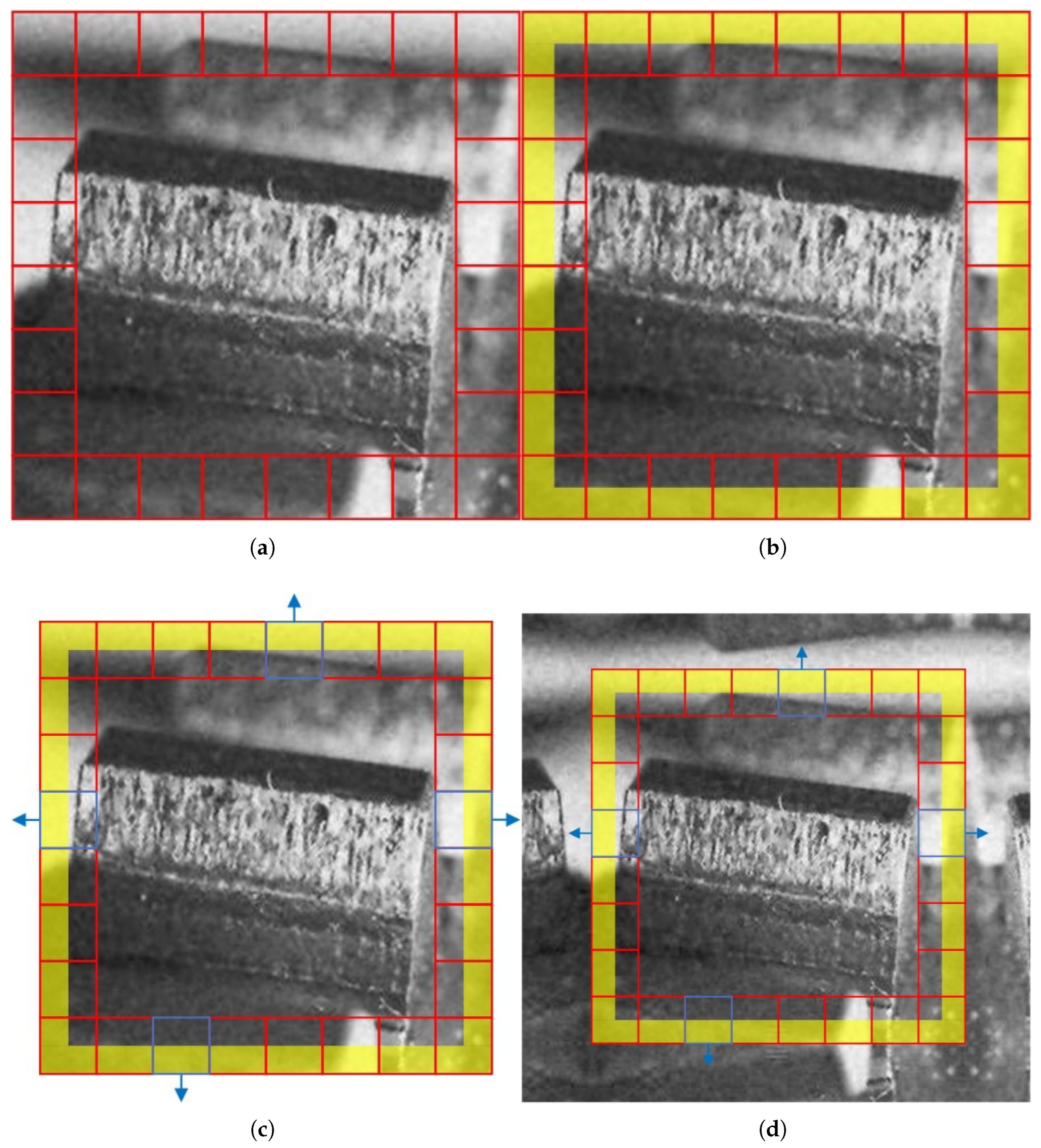
Figure 2.
Example of an extreme case.

Figure 3.
Flow chart of the BELCD Method.
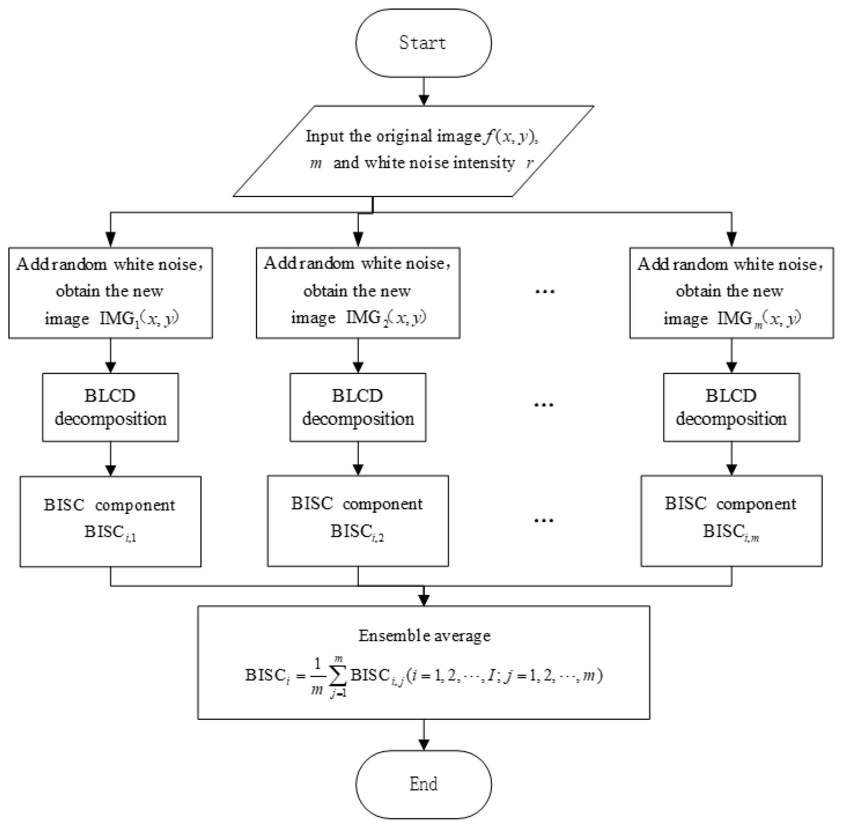
Figure 4.
Flow chart of the BCELCD Method.
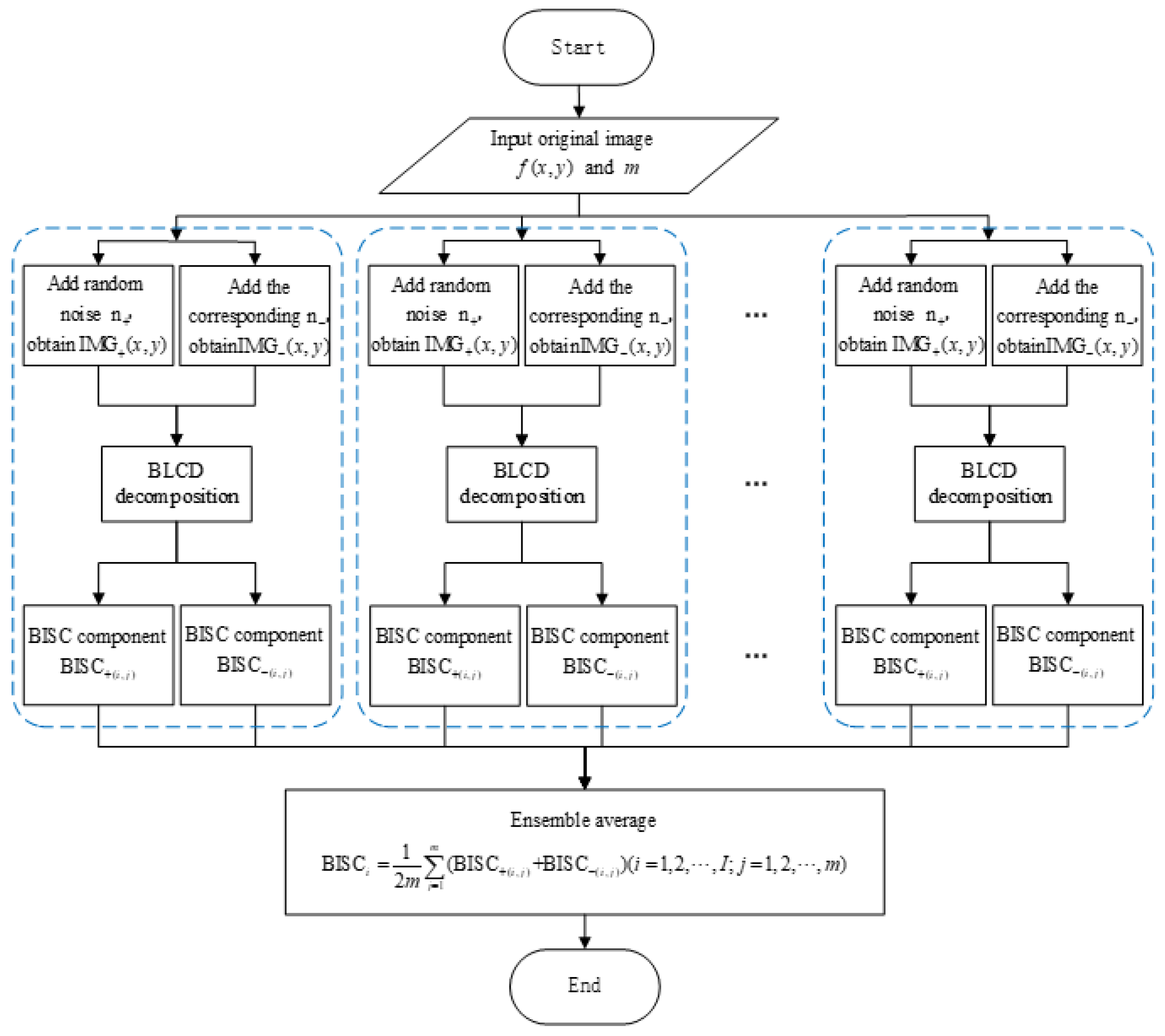
Figure 5.
Flow chart of the BCELCDAN Method.
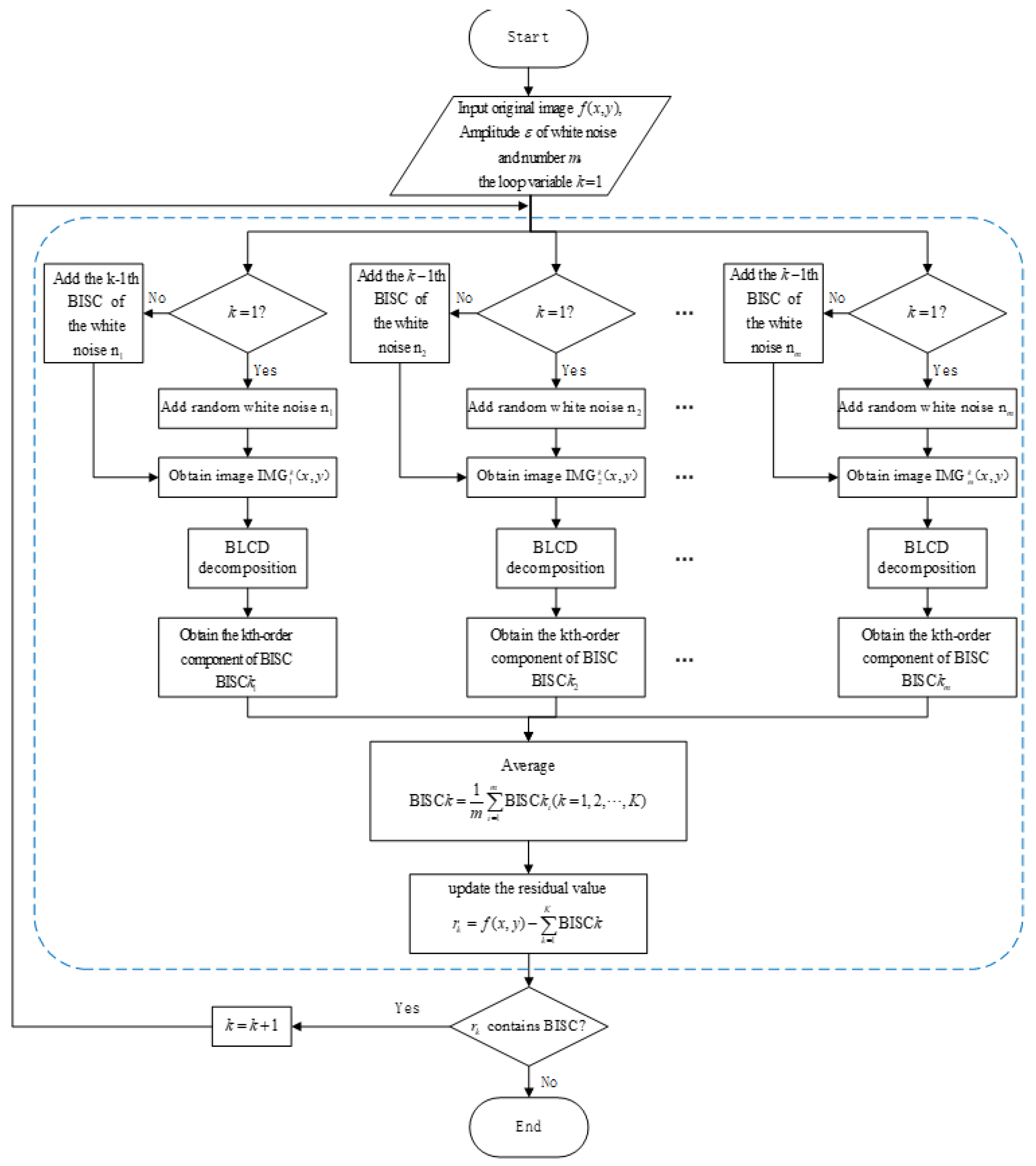
Figure 6.
Different data augmentation results for a normal mode gear surface image from the dataset: (a) Original image, (b) Motion blur, (c) Gaussian blur, (d) Color temperature adjustment, (e) Adaptive histogram equalization, (f) Horizontal flip, (g) Vertical flip, (h) Non-uniform scaling, (i) Perspective transformation, (j) Random contrast, (k) Edge enhancement, (l) Random cropping and padding
Figure 6.
Different data augmentation results for a normal mode gear surface image from the dataset: (a) Original image, (b) Motion blur, (c) Gaussian blur, (d) Color temperature adjustment, (e) Adaptive histogram equalization, (f) Horizontal flip, (g) Vertical flip, (h) Non-uniform scaling, (i) Perspective transformation, (j) Random contrast, (k) Edge enhancement, (l) Random cropping and padding
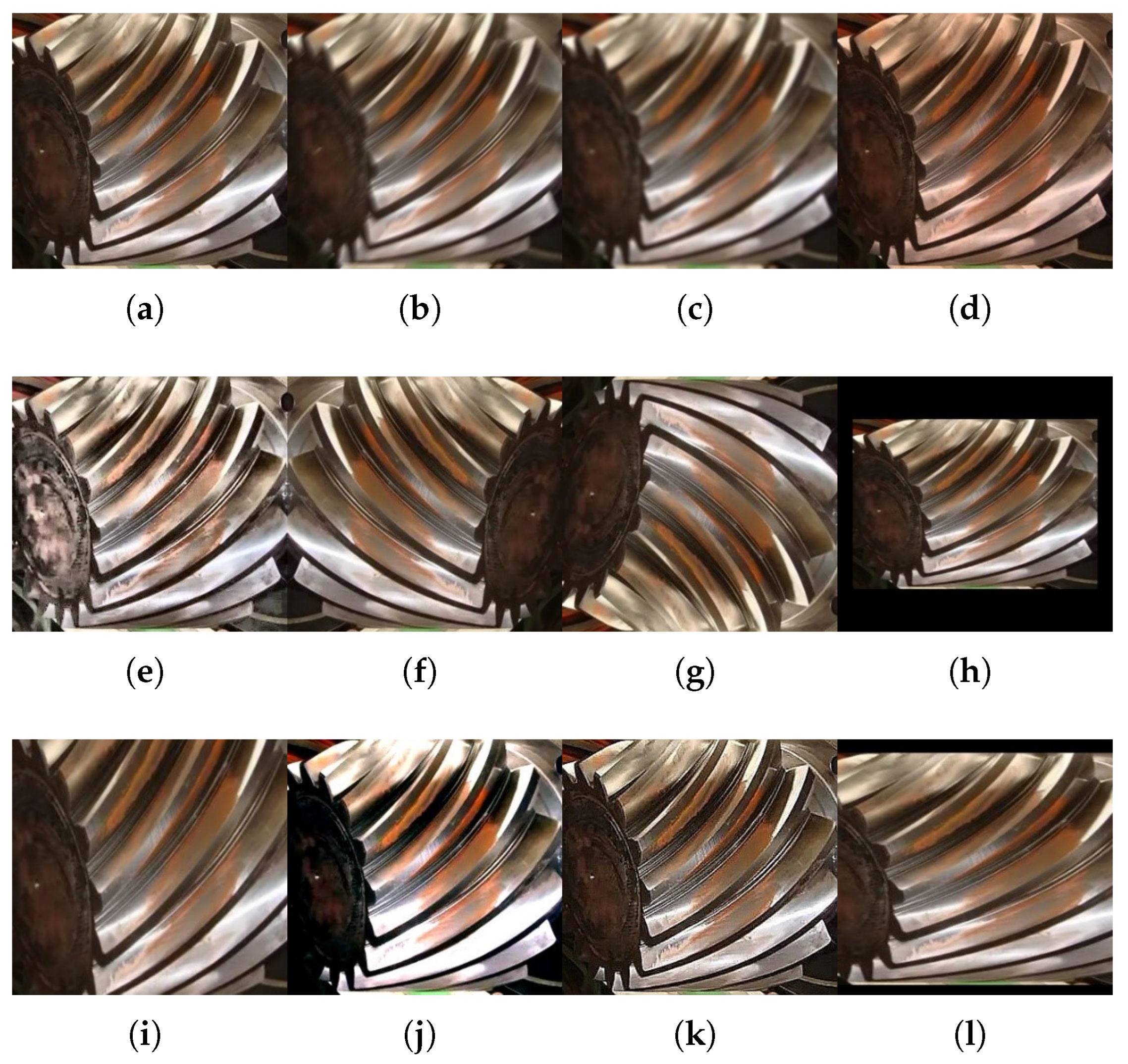
Figure 7.
A grayscale image from the dataset.
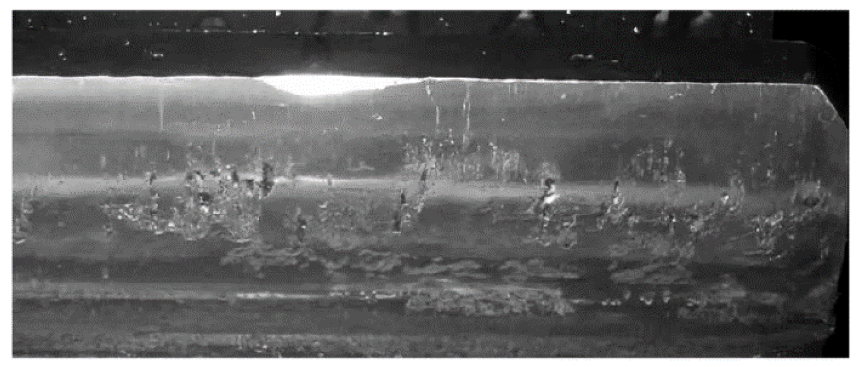
Figure 8.
Grayscale image of gear pitting with random noise.
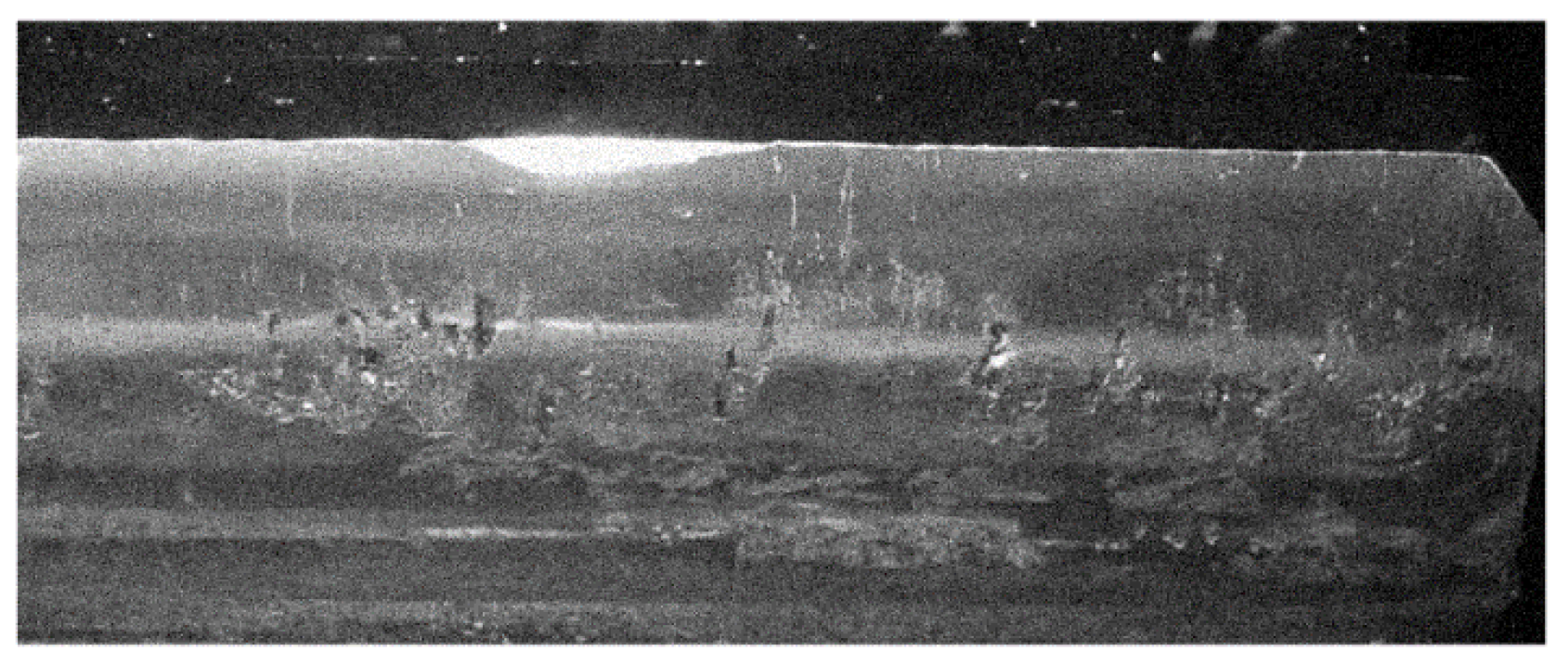
Figure 9.
A set of denoising results: (a) Improved BLCD image denoising, (b) BLCD-based image denoising, (c) BEMD-based image denoising, (d) Median filtering, (e) Adaptive Wiener filtering, (f) Wavelet denoising (global thresholding).
Figure 9.
A set of denoising results: (a) Improved BLCD image denoising, (b) BLCD-based image denoising, (c) BEMD-based image denoising, (d) Median filtering, (e) Adaptive Wiener filtering, (f) Wavelet denoising (global thresholding).
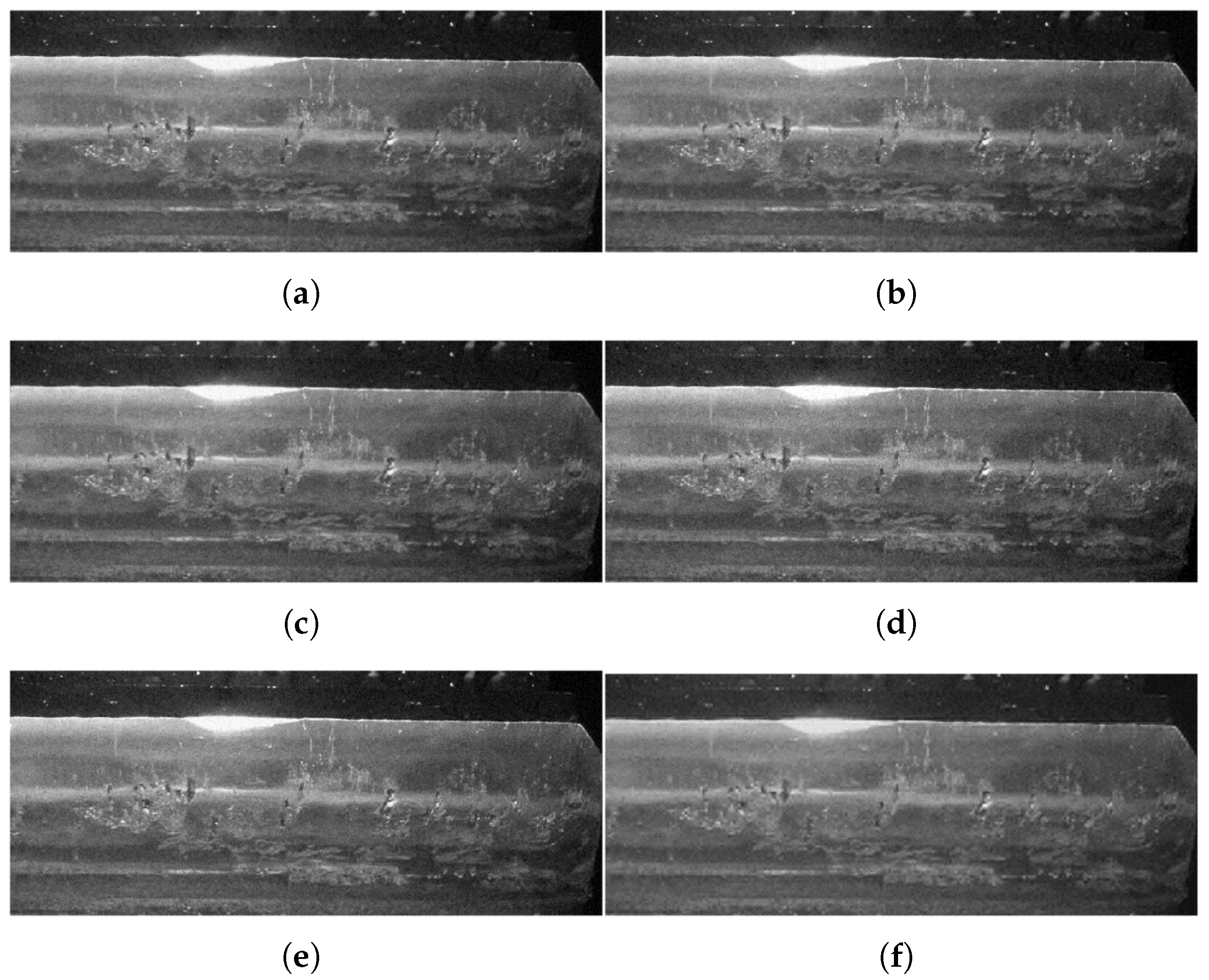
Figure 10.
Confusion matrix results of the comparison experiment: (a) Improved BLCD denoising module + VGG16 detection module, (b) BLCD denoising module + VGG16 detection module.
Figure 10.
Confusion matrix results of the comparison experiment: (a) Improved BLCD denoising module + VGG16 detection module, (b) BLCD denoising module + VGG16 detection module.
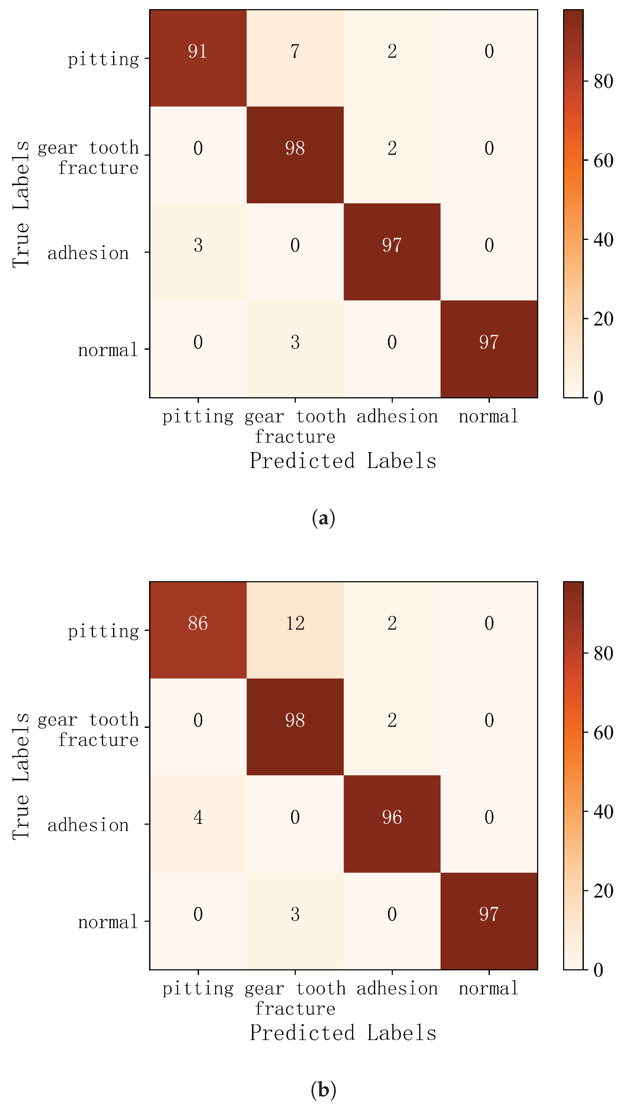

Table 1.
Structural Similarity between the First-Order Component of Each Method and the Reference Component at Different Noise Addition Counts.
Table 1.
Structural Similarity between the First-Order Component of Each Method and the Reference Component at Different Noise Addition Counts.
| Number of Noise Additions | Decomposition Method | ||
|---|---|---|---|
| BELCD | BCELCD | BCELCDAN | |
| 5 | 0.7369 | 0.7309 | 0.7333 |
| 10 | 0.8327 | 0.8359 | 0.8361 |
| 15 | 0.8747 | 0.8737 | 0.8743 |
| 20 | 0.8960 | 0.8944 | 0.8952 |
| 25 | 0.9078 | 0.9078 | 0.9098 |
| 30 | 0.9187 | 0.9188 | 0.9190 |
| 35 | 0.9249 | 0.9245 | 0.9263 |
| 40 | 0.9316 | 0.9308 | 0.9299 |
| 45 | 0.9349 | 0.9347 | 0.9353 |
| 50 | 1.000 | 1.000 | 1.000 |
Table 2.
Structural similarity between reconstructed images of each method and the reference image under different noise addition counts.
Table 2.
Structural similarity between reconstructed images of each method and the reference image under different noise addition counts.
| Number of Noise Additions | Decomposition Method | ||
|---|---|---|---|
| BELCD | BCELCD | BCELCDAN | |
| 5 | 0.8865 | 0.8876 | 1.0000 |
| 10 | 0.9325 | 0.9333 | 1.0000 |
| 15 | 0.9497 | 0.9503 | 0.8743 |
| 20 | 0.9590 | 0.9589 | 0.8952 |
| 25 | 0.9645 | 0.9648 | 0.9098 |
| 30 | 0.9683 | 0.9686 | 0.9190 |
| 35 | 0.9712 | 0.9709 | 0.9263 |
| 40 | 0.9733 | 0.9733 | 0.9299 |
| 45 | 0.9747 | 0.9748 | 0.9353 |
| 50 | 1.000 | 1.000 | 1.000 |
Table 3.
Evaluation Metrics of Various Denoising Methods.
| Evaluation Criteria | Index | ||||
|---|---|---|---|---|---|
| MSE | PSNR | IFC | VIF | SSIM | |
| Original Noisy Image | 70.361 | 23.128 | 1.468 | 0.319 | 0.320 |
| Improved BLCD Image Denoising Method | 17.939 | 31.651 | 1.765 | 0.367 | 0.805 |
| BLCD-based Image Denoising Method | 18.112 | 31.564 | 1.761 | 0.367 | 0.804 |
| BEMD-based Image Denoising Method | 15.062 | 31.256 | 1.766 | 0.367 | 0.806 |
| Median Filtering | 29.836 | 29.694 | 1.507 | 0.322 | 0.685 |
| Adaptive Wiener Filtering | 25.456 | 30.217 | 1.699 | 0.361 | 0.710 |
| Wavelet Denoising (Global Threshold) | 31.806 | 27.625 | 1.179 | 0.239 | 0.781 |
Table 4.
Comprehensive evaluation metrics of the confusion matrix for the comparison experiment.
| Evaluation Criteria | Index | |||
|---|---|---|---|---|
| Accuracy | Macro-precision | Macro-recall | Macro-F1 score | |
| Improved BLCD denoising module + VGG-16 detection module | 95.75% | 95.90% | 95.75% | 0.9537 |
| BLCD denoising module + VGG-16 detection module | 94.25% | 94.57% | 94.25% | 0.9426 |
Disclaimer/Publisher’s Note: The statements, opinions and data contained in all publications are solely those of the individual author(s) and contributor(s) and not of MDPI and/or the editor(s). MDPI and/or the editor(s) disclaim responsibility for any injury to people or property resulting from any ideas, methods, instructions or products referred to in the content. |
© 2026 by the authors. Licensee MDPI, Basel, Switzerland. This article is an open access article distributed under the terms and conditions of the Creative Commons Attribution (CC BY) license (http://creativecommons.org/licenses/by/4.0/).
Copyright: This open access article is published under a Creative Commons CC BY 4.0 license, which permit the free download, distribution, and reuse, provided that the author and preprint are cited in any reuse.


