
Submitted:
03 January 2026
Posted:
06 January 2026
You are already at the latest version
Abstract
The Plastino-Plastino Equation (PPE) is essential in non-extensive statistics in the study of systems that exhibit anomalous diffusion and do not fit conventional statistics, thus being a nonlinear extension of the Fokker-Planck Equation (FPE). This equation has been applied in various fields of physics (Cosmology, astrophysics and hadrons, specifically in Quark-Gluon Plasma) and other disciplines. In this work, a relativistic approach will be carried out on a system of particles for which the relativistic Boltzmann equation is obtained. Here, grazing collisions are considered to obtain the FPE integrated with special relativity. Subsequently, through fractal derivations, a modification of the FPE is made, resulting in the PPE in a relativistic context.
Keywords:
fractal
; Plastino-Plastino
; Fokker-Planck
; relativistic
1. Introduction
The Boltzmann equation is a cornerstone of nonequilibrium statistical mechanics, allowing for the dynamical evolution of a distribution function , which describes how a system of particles evolves through collisions by quantifying the particles’ positions and velocities [1,2,3]. This equation has found applicability in many systems, including those at relativistic energies, an extension that was made possible by incorporating relativity. Thus, the Boltzmann equation is now applied in astrophysics, in studies of the early universe, and in investigations of the Quark-Gluon Plasma (QGP) [4,5,6]. Another very common application of the relativistic Boltzmann equation is in the area of electromagnetic plasmas [7].
The Fokker-Planck Equation (FPE) can be derived from the Boltzmann equation through a second-order expansion of the probability density, resulting in a second-order differential equation that describes the statistical behaviour of the system through transport coefficients: the drag (or drift) coefficient, associated with external forces, and the diffusion coefficient, associated with stochastic collisions among the many particles in the system [8,9]. This equation must be covariant under Lorentz transformations to be applied to relativistic systems [10,11]. Among its applications is plasma physics, allowing the analysis of the dynamics of charged particles, as well as astrophysics and cosmology, where the evolution of nebulae is studied. All these systems are subject to the combined effects of drag and relativistic diffusion [12,13]. With such an extension, the transport coefficients must be reinterpreted in terms of the exchange of four-momentum during particle interactions.
The FPE, however, is restricted to a particular class of systems, namely those for which the collision term of the Boltzmann equation has a correlation functional that is bilinear in the interacting particle distributions. This assumption is useful and valid for interactions that are local, uncorrelated, and follow a Markovian sequence. However, there is increasing interest in systems that fall outside this class and are instead described by nonlinear Fokker-Planck equations. Within this family of nonlinear equations, a particular class is of broad applicability, namely the Plastino-Plastino Equation (PPE) [14], which was proposed in connection with systems following Tsallis statistics [14,15,16,17].
Tsallis statistics has been applied in different fields of physics and beyond, yielding numerous studies, especially in high-energy physics. The emergence of Tsallis statistics in quantum field theory can be traced to the renormalisation properties of these theories and to self-energy interactions. Together, these properties provide the necessary conditions for the formation of thermofractals [18], and their mathematical tools have uncovered a deep relationship between the Tsallis index q and field-theoretical parameters, which in the case of QCD are the number of colours and flavours. This connection has shown that q is a structural parameter within quantum field theory, rather than merely a fitting parameter.
The description of the dynamics of heavy quarks in the QGP within this statistical framework, particularly through the PPE [14], is of great importance. This nonlinear dynamics, within nonextensive statistics, provides a means to describe the evolution of complex and random systems and has proven relevant in research across different areas of physics [17]. Recently, the PPE was used to investigate the dynamical origin of the nuclear modification factor in high-energy nuclear collisions [19] by employing a nonrelativistic version of the equation. Although relativistic effects may be limited in some cases, it is important to extend the PPE so that it behaves covariantly under Lorentz transformations.
In this work, a derivation of the PPE is carried out by incorporating special relativity, leading to the Relativistic Plastino-Plastino Equation (RPPE) within the framework of Tsallis q-statistics. The paper is structured as follows: Section 2 derives the relativistic Boltzmann equation for a particle collision system. In addition, the relativistic Fokker-Planck equation is deduced from the relativistic Boltzmann equation, and in Section 4, the RPPE is derived from the RFPE using fractal derivatives, ultimately yielding a relativistic equation expressed in terms of the velocity variable. Final remarks are presented in Section 5.
2. Relativistic Boltzmann and Fokker-Planck Equations
A particle of rest mass m is described by the space-time coordinates and by the four-momentum , where is given by . The one-particle distribution function, defined in terms of space-time and momentum coordinates as , is such that
where t is the instant at which the number of particles in a volume element around and with momentum within around is measured [1]. The number of particles in the volume is a scalar invariant, since all observers count the same number of particles. Therefore, the distribution function is itself a scalar invariant [1].
Defining the phase-space volume at time t as , the number of particles in this volume is
At time , the number of particles becomes
Due to particle collisions, , and the variation is
where the increments in the position and in the momentum are given as,
The relationship between and is given by, with J denoting the Jacobian of the transformation,
The increments in position and momentum are and , where is the external force and is the particle velocity [1]. The Jacobian relating and is
with .
Expanding to first order in yields
Since and the proper time are scalar invariants,
is a scalar invariant as well as the proper time , hence
is a scalar invariant [1]. Where is a scalar invariant, and as a consequence the expression multiplying, must have the same property. We first consider the term
in which and multiplying and dividing the first term by , we have that
Since f is a scalar invariant, is a 4-vector, and the scalar product is a scalar invariant. We consider the Minkowski force defined by
that satisfies, and the relationship,
If we consider as an independent variable and make use of the chain rule:
To determine , we decompose it in two terms
where corresponds to the particles that leave the volume , whereas corresponds to those particles that enter in the same volume. Further, we assume the following:
- a)
- b)
- If and denote the momenta of two particles before collision they are not correlated. This will be applied to the momenta of the particle that we are following, and of its collision partner, as well as to two momenta and , possessed by two particles before a collision that will transform them into particles with momenta and after collision [1].
- c)
- The one-particle distribution function does not vary very much over a time interval which is larger than the duration of a collision but smaller the time between collisions. The same applies to the change of over a distance of the order of the interaction range [1].
We consider a collision between two beams of particles with velocities and . The particle number densities of these two beams in their own frames are denoted by and . The d in front of n and indicates that these number densities are infinitesimal because they refer to volume elements and of momentum space ( and ) [1].
The total number of particles around is . The total number of particles that collide in the volume will be , where is the relative velocity and is a proper volume [1].
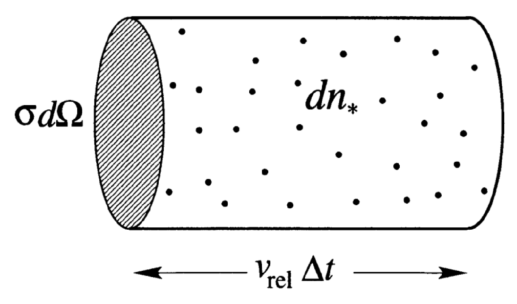
The particles with density in the volume are differently scattered by their partners in the collision through different angles. Each collision will occur in a plane with some scattering angle ; another angle is needed to single out the plane and two infinitesimal neighborhoods of the two angles together single out a solid angle element [1]. The volume element can be written in terms of the so-called collision cylinder of base and height . is identified with the differential of the proper time, because of the choice of the reference frame. The factor has clearly the dimensions of an area and is called the differential cross-section of the scattering process corresponding to the relative speed and the scattering angle . In another reference system where , , , and are scalar invariants [1].
The total number of collisions will be given then by the product of the particle numbers corresponding to the velocities and (See Figure 2):
where we have rewritten the volume element in terms of the collision cylinder. Let us consider the product of the particle number densities in a system where :
We have that the total number of collisions given by Eq. (20) is
In which another form of relative speed is used, known as Mller relative velocity,
then,
where we have introduced Mller´s relative velocity [1]. Now the total number of particles that leave the volume is obtained by integrating it over all momenta and over all solid angle , yielding
This is frequently called the loss term because it describes the loss of particles in the volume in phase space, due to collisions. We consider a collision between two beams of particles with velocities and and we write the total number of particles that leave the volume element as,
which is called the gain term since it describes the gain of particles in the volume element . For relativistic particles we have that [1]. Therefore, through Liouville’s theorem, it is obtained that the volume in phase space does not change over time. Here, we have that
since is an invariant, we have that
3. Relativistic Fokker-Planck Equation
Under the assumption of grazing collisions that could take place in long-range interactions, only small changes in the momentum of the particles occur due to small deflections in the scattering angle. Then the collision term of the Boltzmann equation, denoted by [7]. The total and the relative four-momentum, defined by
For these quantities the following relationships hold are,
The differences between the post- and pre-collision four-momentum,
Hence for small changes of the momentum of the particles at collision one can expand the one-particle distribution function in Taylor series, which up to the second-order terms,
with a similar expression for . Now it is possible to approximate the collision term of the Boltzmann equation as [7],
then, introducing Eq. (37), with the help of the relationship,
then,
In order to transform the integral, the center-of-mass system is chosen where the spatial components of the total four-momentum vanish, i.e., and . Now the element of solid angle can be written as , where and are polar angles of with respect to and such that represents the scattering angle [7]. Further, without loss of generality, is chosen in the direction of the three axis, so that one can write and as
by using the above representations, the integrals in the variable , yielding
where and . Note that the differential cross-section is a function of . Then,
where
then,
and are the spatial components of the metric tensor [7]. By differentiating with respect to , we have
here we have used Eq. (45), therefore,
therefore,
where and using Eq. (47), we have that
The first term on the right-hand side of the above equation vanishes, since the hypothesis of grazing collisions is used and it is possible to convert; thanks to the divergence theorem; the volume integral in the momentum space into an integral at an infinitely far surface where the distribution functions tend to zero [7]. By invoking the divergence theorem again,
where the spatial components of the coefficient of dynamic friction and the diffusion coefficient are given by
In this system , and one can include the zero components
Hence the Relativistic Boltzmann Equation reduces to the Relativistic Fokker-Planck Equation, namely [7]
4. Relativistic Plastino-Plastino Equation
The Relativistic Plastino-Plastino Equation is derived from the Relativistic Fokker-Planck equation given in Eq. (53). We consider the spatially homogeneous case without external forces, which reduces the relativistic Fokker-Planck equation to
Here, fractal derivatives are employed. More specifically, ordinary derivatives are replaced by fractal derivatives, transforming the above equation into
where denotes the fractal derivative and , with q being the Tsallis entropic index, thus establishing the connection with nonextensive statistics.
Starting from
where and , which relates ordinary differentiation to fractal differentiation, Eq. (55) is modified, yielding
which is the Relativistic Plastino-Plastino Equation.
4.1. Rapidity Space
A useful modification of the Relativistic Plastino-Plastino Equation involves the rapidity variable, placing Eq. (57) fully within a relativistic framework. Using natural units, , we have
Introducing the change of variables and [20], the above equation becomes
and therefore
which is the Plastino-Plastino equation expressed in terms of the rapidity variable.
5. Conclusions
This work provides the first demonstration of the Relativistic Plastino-Plastino Equation derived from the Relativistic Boltzmann Equation. Initially, the relativistic version of the Fokker-Planck equation is obtained, and it is then shown that this equation is limited to a specific form of correlators in the collision term. As a consequence, it cannot be applied to systems that do not follow a Markovian sequence of collisions, such as systems exhibiting memory effects or nonlocal correlations.
Motivated by recent results, this work identifies the Plastino-Plastino Equation as the appropriate framework for describing systems with such characteristics, including quark-gluon plasma, hadronic systems, and electromagnetic plasmas. Following the methodology of previous studies, the Relativistic Plastino-Plastino Equation is derived from the relativistic Fokker-Planck equation by exploiting the known connections between the fractal Fokker-Planck equation and the Plastino-Plastino Equation. These connections rely on the recently established relationship between fractal derivatives and q-deformed derivatives.
The relativistic version of the Plastino-Plastino Equation opens new possibilities for investigating the dynamical evolution of systems such as solar plasmas, Tokamak plasmas, quark-gluon plasma, and neutron star cores. The use of the relativistic formulation enables more precise analyses and a more accurate determination of the key physical parameters governing these systems.
Funding
This research was funded by the Conselho Nacional de Desenvolvimento Científico e Tecnológico (CNPq-Brazil).
Data Availability Statement
All data generated or analyzed during this study are included in this article. The data used to support the findings of this study are included within the article and properly cited.
Acknowledgments
The research of A.D. and J.M.C. was funded by the Conselho Nacional de Desenvolvimento Científico e Tecnológico (CNPq-Brazil). This work was supported by CNPq, grant numbers 306093/2022-7 and 140711/2022-8, and FAPESP, grant numbers 2024/01533-7 and 2025/22475-8.
Conflicts of Interest
The authors declare no conflicts of interest.
Abbreviations
The following abbreviations are used in this manuscript:
| FPE | Fokker-Planck Equation |
| RFPE | Relativistic Fokker-Planck Equation |
| PPE | Plastino-Plastino Equation |
| RPPE | Relativistic Plastino-Plastino Equation |
| QGP | Quark-Gluon Plasma |
References
- Cercignani, C.; Kremer, G.M. Relativistic Boltzmann Equation. In The Relativistic Boltzmann Equation: Theory and Applications; Progress in Mathematical Physics; Birkhäuser: Basel, 2002; vol 22. [Google Scholar]
- de Groot, S. R.; van Leeuwen, W. A.; van Weert, Ch. G. Non-Equilibrium relativistic kinetic theory-principles and applications; North Holland: Amsterdam, 1980. [Google Scholar]
- Horwitz, L. P. The relativistic Boltzmann equation and two times. Entropy 2020, vol. 22(no. 8). [Google Scholar] [CrossRef] [PubMed]
- Mendenhall, T.; Lin, Z.-W. Effectiveness of parton cascade in solving the relativistic Boltzmann equation in a box. Nucl. Phys. B 2025, vol. 1022, 117242. [Google Scholar] [CrossRef]
- Enomoto, S.; Su, Y.-H.; Zheng, M.-Z.; Zhang, H.-H. Boltzmann Equation and Its Cosmological Applications. Symmetry 2025, vol. 17(no. 6). [Google Scholar] [CrossRef]
- Colonna, G. Boltzmann and Vlasov equations in plasma physics. In Plasma Modeling (Second Edition); IOP Publishing, 2022; Volume 2053-2563, p. 1-1 to 1-25. [Google Scholar]
- Kingham, R.J.; Bell, A.R. An implicit Vlasov–Fokker–Planck code to model non-local electron transport in 2-D with magnetic fields. Journal of Computational Physics 2004, Vol. 194, 1–34. [Google Scholar] [CrossRef]
- Debbasch, F.; Mallick, K.; Rivet, J.P. Relativistic Ornstein–Uhlenbeck Process. Journal of Statistical Physics 1997, 88, 945–966. [Google Scholar] [CrossRef]
- Medved, A.; Davis, R.; Vasquez, P. A. Understanding Fluid Dynamics from Langevin and Fokker–Planck Equation. Fluids 2006, vol. 5(no. 1). [Google Scholar] [CrossRef]
- van Hees, H.; Greco, V.; Rapp, R. Heavy-quark probes of the quark-gluon plasma at RHIC. Phys. Rev. C 2006, vol. 73, 034913. [Google Scholar] [CrossRef]
- Chacón-Acosta, G.; Kremer, G. M. Fokker-Planck-type equations for a simple gas and for a semirelativistic Brownian motion from a relativistic kinetic theory. Phys. Rev. E 2007, vol. 76, 021201. [Google Scholar] [CrossRef] [PubMed]
- Felix, J. A. A.; Calogero, S. On a relativistic Fokker-Planck equation in kinetic theory. Kin. Rel. Mod. 2011, vol. 4, 401–426. [Google Scholar]
- Bornatici, M. Relativistic Fokker-Planck equation for electron cyclotron radiation. Physica Scripta 1994, vol. 1994, 38. [Google Scholar] [CrossRef]
- Plastino, A.; Plastino, A. Non-extensive statistical mechanics and generalised Fokker-Planck equation. Phys. A: Statistical Mechanics and its Applications 1995, vol. 222(no. 1), 347–354. [Google Scholar] [CrossRef]
- Tsallis, C. Possible Generalization of Boltzmann-Gibbs Statistics. J. Statist 1988, vol. 52, 479–487. [Google Scholar] [CrossRef]
- Deppman, A.; Megías, E.; P. Menezes, D. Fractal Structures of Yang–Mills Fields and Non-Extensive Statistics: Applications to High Energy Physics. Physics 2020, 2, 455–480. [Google Scholar] [CrossRef]
- de Luca, V. T. F.; Wedemann, R. S.; Plastino, A. R. The nonlinear Fokker–Planck equation with nongradient drift forces and an anisotropic potential. Chaos: An Interdisciplinary Journal of Nonlinear Science 2025, vol. 35, 093115. [Google Scholar] [CrossRef] [PubMed]
- Deppman, A. Thermodynamics with fractal structure, Tsallis statistics, and hadrons. Physical Review D 2016, 93, 054001. [Google Scholar] [CrossRef]
- Baptista, R.; Rocha, L. Q.; Pareja, J. M. C.; Bhattacharyya, T.; Deppman, A.; Megías, E.; Rybczyński, M.; Wilk, G.; Włodarczyk, Z. Nuclear modification factor within a dynamical approach to the complex entropic index. The European Physical Journal A 2025, 61, 271. [Google Scholar] [CrossRef]
- Collins, J. C. hep-ph/9705393; Light cone variables, rapidity and all that. 1997.
- Megias, E.; Deppman, A.; Pasechnik, R.; Tsallis, C. Comparative study of the heavy-quark dynamics with the Fokker-Planck equation and the Plastino-Plastino equation. Phys. Lett. B 2023, vol. 845, 138136. [Google Scholar] [CrossRef]
- Megias, E.; Khalili Golmankhaneh, A.; Deppman, A. Dynamics in fractal spaces. Phys. Lett. B 2024, vol. 848, 138370. [Google Scholar] [CrossRef]
- Megias, E.; Deppman, A.; Pasechnik, R. Fractal Derivatives, Fractional Derivatives and q-Deformed Calculus. Entropy 2023, vol. 25(no. 7). [Google Scholar]
- Plastino, A. R.; Plastino, A. Non-extensive statistical mechanics and generalized Fokker–Planck equation. Physica A 1995, vol. 222, 347–354. [Google Scholar] [CrossRef]
Figure 1.
Schematic representation of a binary collision.
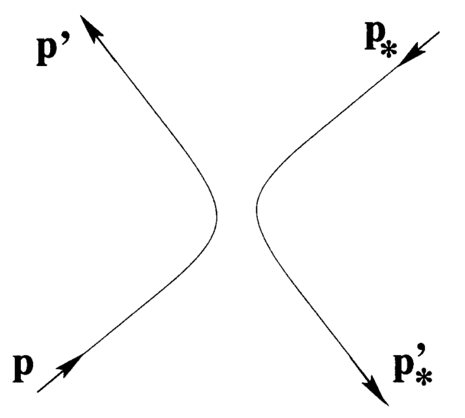
Figure 2.
Schematic representation of the collision cylinder.
Disclaimer/Publisher’s Note: The statements, opinions and data contained in all publications are solely those of the individual author(s) and contributor(s) and not of MDPI and/or the editor(s). MDPI and/or the editor(s) disclaim responsibility for any injury to people or property resulting from any ideas, methods, instructions or products referred to in the content. |
© 2026 by the authors. Licensee MDPI, Basel, Switzerland. This article is an open access article distributed under the terms and conditions of the Creative Commons Attribution (CC BY) license (http://creativecommons.org/licenses/by/4.0/).
Copyright: This open access article is published under a Creative Commons CC BY 4.0 license, which permit the free download, distribution, and reuse, provided that the author and preprint are cited in any reuse.


