
Submitted:
05 January 2026
Posted:
05 January 2026
You are already at the latest version
Preprints on COVID-19 and SARS-CoV-2
Abstract
This paper focuses on analyzing the dynamic process, strength and orientation of risk spillovers in the Chinese banking system under the exogenous shock scenario of the COVID-19 pandemic. Using the closing prices of 25 chosen banks on a daily basis, it stratifies the data into three periods: before, during, and after the pandemic. The HP-TVP-VAR-DY model is used to model risk heterogeneity and time-varying features in risk transmission processes. A dynamic topological directional graph is further used to track the core risk sources and paths in risk transmission processes. The key findings obtained from this paper are summarized below: (1) The Total Spillover Index for the banking system persisted at a high level following the outbreak of the COVID-19 pandemic, indicating its high sensitivity to abrupt and large-scale events. (2) Bank risk transmission paths are highly heterogeneous and time-varying in nature. Prior to the pandemic, CCBs were prominent in overall risk output; during the pandemic, JSCBs dominated; while in the post-pandemic period, again CCBs dominated overall risk output. In all periods, SOCBs and RCBs were identified as major risk receivables. (3) Concerning the structural change in interbank risk transmission paths, it exhibits phase-dependent features. In the pre-pandemic period, risk spillovers spread from CIB, CMB to ABC. However, in the pandemic period, interbank risk transmission paths became highly decentralized, indicating significant increases in risk outflows and inflows from RCBs and CCBs, respectively. Moreover, CMBC and SZRCB turned out to become key sources for risk radiation, while overall network mechanisms dominated risk absorption effects. However, in the post-pandemic period, interbank risk transmission paths tend to become re-centralized; BOC turned out to become a core source for risk transformation, indicating a revival in risk-output dominance in network topologies.
Keywords:
HP-TVP-VAR-DY
; COVID-19 pandemic
; Complex networks
; Risk spillovers
; Systemically Important Banks
; Core risk sources
1. Introduction
The Global Financial Crisis in 2008 underlined the potential dangers of risk contagion in a global economy. Related to China’s bank-based structure in a global economy, there is a close nexus between macroeconomic instability and banking system stability in China.
Heterogeneity in the value of assets, business types and respective risk exposures induces banks to undertake different systemic roles in the financial structure. If a shock emerges in a particular bank, such as liquidity crisis or credit risk, this event develops rapidly into a process influencing other banks via interbank transactions, payment and settlement processes, as well as asset price volatility. Such a situation generates the so-called “domino effect”. The process of potential transitions from idiosyncratic to systemic risk endangers the existence of particular institutions, including banks, but also has the potential for generating systemic crisis processes within the banking sector. In extreme cases, it might influence the process of chain reactions occurring within the complete financial structure, thereby strongly hindering the usual course of economic processes within the real economy. Therefore, under extreme stress conditions, it is crucial to identify properly the transmission paths, mechanisms and processes of risk development among heterogeneous banking institutions, and explain the dominant risk sources, as well as the primary transmission paths within this financial structure.
Considerable literature has explored the risk spillovers of the financial system from different views and methodologies. For instance, from the perspective of complex network theory, Allen [1] studied the risk contagion effect on the overall financial system through interbank exposure data. Then, there is the financial network model of interbank lending games proposed by Fan [2] , indicating that risk contagion can form multiple lending equilibria in the interbank market. Regarding tail risk literature, Yang [3] employed the GARCH-Copula-CoVaR model to study the systemic financial risk of 16 listed Chinese commercial banks. The TENET approach was then used in Zhang [4], who estimated the network properties and financial risk contributions of China’s Systemically Important Banks during extreme scenarios. Moreover, there are researchers who target the creation of systemic risk measures. For example, Ma [5] carried out scenario analysis and stress testing of 45 commercial banks. The research aimed at pointing out that asset liquidity has an important role in risk contagion. Another example is Liang [6], who presented the SRISK indicator to evaluate systematically important financial institutions.
Among these methodologies, the use of network analysis has gained remarkable momentum over the past few years. Diebold & Yilmaz [7] developed the Generalized Variance Decomposition Framework that helped identify global complex networks. This was followed by the expansion of different models. For instance, Time Varying Parameter Vector Autoregressive (TVP-VAR) models that take into consideration the variation in parameters for different periods have gained remarkable importance. This was first done by Antonakakis et al. [8]. Since then, different models have followed this methodology [9,10,11,12]. However, these models use rolling window for estimation. This results in the reduction of the sample observations. To counter this drawback, the TVP-Quantile-VAR-DY model was developed[13]. This partially overcame the problem of reduction in sample observations.
It is important to highlight the fact that complex networks have two inherent characteristics: time-variability and high-dimensionality. Both features are considered the most challenging for the common approaches and techniques. Though TVP-VAR-DY class models are very effective in the time-variant structures, they have some limitations in dealing with high-dimensional variables. Currently, the solution for the high-dimensional problems basically falls into two categories. The standard TVP-VAR-DY models are generally constrained by computer complexity, which may not exceed twenty variables, while some cases may even forgo variables in order for the model to retain its TVP nature. However, in the alternative method, dimensionality reduction techniques are used to enhance model power. For instance, the Lasso-VAR-DY model developed by Demirer et al. [14] uses LASSO to reduce coefficients, thus suppressing bias in model estimation due to high dimensionality. However, when highly correlated variables are involved, LASSO may encounter instabilities in coefficient selection, hence affecting efficiency in estimation.
To address the high dimensionality and heterogeneity issue, Chen [15] further developed the HD-TVP-VAR-DY model. Based on the Diebold-Yilmaz index of spillovers, this model combines the Kalman filter and the Elastic Net algorithm. Compared with traditional TVP-VAR-DY models, the HD-TVP-VAR-DY model is capable of processing time-varying relationships among almost 100 variables. This is achieved without losing the individual variability in the data and without the losses entailed in rolling window estimations. This shows notable improvements in both the estimation speed and computing speed.
In summary, although recent studies do investigate the dynamic processes for risk contagion between banks triggered by sudden events[16,17,18], the studies conducted in this area are still few. There exists a significant lack of refined definition concerning the paths of risk transmission for different types of banks. In order to bridge this gap, the study uses the HD-TVP-VAR-DY framework for an in-depth analysis. From the methodological viewpoint, the study has three strengths. First, by allowing the individual banks to have their own set of equation coefficients, the study takes into consideration the heterogeneity present in the banking sector. Second, it identifies the smooth and continuous process of the evolution of the parameters over the timeline, thereby capturing the exact dynamics of the intensity of the risk contagion process in the pre-pandemic, pandemic, and post-pandemic periods. Third, it converts the associations into the form of specific spillover matrices and also unfolds the dynamic directed networks to pinpoint the core risk sources and transmission paths in the system.
In comparison with the existing literature, the marginal contributions of this study are as follows: (1) The use of the HD-TVP-VAR-DY model increases the sample size to 25 banks, enabling a comprehensive description of the time-varying and high-dimensional properties within the complex network. (2) Based on the consideration of the COVID-19 pandemic as an exogenous shock factor, this study conducts an in-depth analysis on the dynamic risk contagion process based on three different phases in time. It reveals disparities in transmission paths, as well as changes in intensity and orientation, thereby contributing to a more detailed description on the structure of risk spillovers in a precise manner in the context of the banking system, providing a reference for the screening and tracking of high-risk banks. (3) The study incorporates the spillover index model with Social Network Analysis. The analysis on dimensions related to centrality within the network enables a systematic definition on core risk sources and critical transmission paths, providing a theoretic foundation on macro-prudential regulation.
2. Materials and Methods
2.1. HD-TVP-VAR-DY Model
The Heterogeneous Dynamic Time-Varying Parameter Vector Autoregression (HD-TVP-VAR) model can be seen as an advanced extension of TVP-VAR. Based on the methodology pioneered in Koop & Korobilis [19], this model brings in heterogeneity in addition to allowing for processing large dimensional datasets in a TVP setup. The general form of this model after demeaning the variables can be expressed by the Equation (1).
where i=1,2,....,N indexes the individual banks (with N=25 in this study), and t = 1, 2,...,T denotes the time period. The variable rit represents the daily return of the i-th bank in the system at time t.The parameterβij,lt denotes the time-varying coefficient capturing the influence of bank j on bank i at lag l during period t, thereby reflecting the magnitude of risk transmission. The parameter p indicates the lag order, and The symbol Σt represents the time-varying covariance matrix.
In order to capture explicitly the heterogeneous properties embedded in the interbank system, the time-varying parameter βij,lt in Equation (1) is decomposed into common and idiosyncratic components, described in Equation (2).
Here, βj,lt represents the common time-varying parameter, which quantifies the average response intensity of the entire banking system to the returns of bank j at lag , thereby capturing systemic common trends.Conversely,βi,lt∗represents the individual idiosyncratic time-varying parameter, measuring the degree of deviation of bank i relative to the system average, thus reflecting the specific heterogeneity of the individual institution.
The dynamic evolution of these parameters is specified as a random walk process, expressed as:
During the start of the shock, the common component βj,lt can grow very fast due to a series of large positive shocks to the innovation variable ηj,lt. Simultaneously, the heterogeneity characteri -stics βi,lt∗of specific banks can go through large structural changes and adjust to new equilibrium values by changing the innovation variable ξi,lt.
With the recognition that the study involves 25 banks and a large number of parameters, this is indeed a classic high-dimensional problem. The direct estimation of high-dimensional problems is predisposed to problems such as overfitting, instability of parameters and multicollinearity, which may render the results of the estimation questionable. To overcome the mentioned difficulties associated with high-dimensional problems, this study applies Elastic Net Regularization to reduce dimensionality. The method includes an additional penalty term to restrict both the size and sparsity of parameters, as defined by Equation (4).
In Equation (4), λ serves as the regularization parameter controlling the shrinkage intensity, the optimal λ is determined via 5-fold cross-validation in this study. The parameter α (0≤α≤1) is the Elastic Net mixing coefficient, balancing the contributions of L1andL2 regularization. The term ‖β‖1 represents the L1 norm,which is the sum of absolute values, promoting sparsity, while ‖β‖22 represents the squared L2 norm,which is the sum of squared values, addressing multicollinearity.
After carrying out dimensionality reduction, there is a need for parameter estimation. Even in existing literature, there is a common practice of using MCMC. However, these techniques are highly dependent on prior distribution and tend to be computationally inefficient when working in high-dimensional spaces. Due to such limitations associated with existing techniques in the literature, this study adopt the Kalman Filter with a Forgetting Factor. This technique was introduced by Chen[20] to overcome the limitations associated with the Kalman Filter. This technique involves the addition of a forgetting factor λ.
The algorithm is comprised of two primary steps: Prediction and Update.
(1) Prediction Step
On the basis of all information available up to time t−1, a prior prediction is made for the state at time t.
State Prediction:
Prediction Covariance Matrix:
As suggested by Equation (6), the uncertainty in the state prediction is contributed by two components: the inherent uncertainty of the estimation at the previous moment and the uncertainty introduced by the stochastic fluctuation of the state equation. In this model, λt is called the forgetting factor, taking on values strictly between 0 and 1. A faster decay of historical data, a higher sensitivity to new information. For this research work, λt varies depending on market fluctuation conditions:
Equation (7) shows that when market volatility increases, it reduces λt. It means that during periods when turbulence is high, the model “forgets” the past more aggressively and places greater weight on current data for parameter updates, making it possible to promptly identify changes in risk contagion mechanisms.
(2) Update Step
Upon receiving new information (yt, Xt), the prior prediction is then updated to generate the posterior prediction.
Kalman Gain:
State Update:
Covariance Update:
Here, the Kalman Gain (Kt) serves as a weighting matrix, determining the extent to which the new observation yt influences the update relative to the prior prediction . This can be deemed as the core mechanism within the Kalman Filter. The State Update (Equation 9) represents the posterior estimate, calculated as the prior estimate plus a correction term. This correction term is the product of the prediction error and the Kalman Gain. With the addition of new information from observed values, the uncertainty of the state estimation is reduced. Pt|t quantifies the precision of the updated estimate .
The Kalman Filter is quite efficient at estimating βij,lt given prior knowledge of covariance matrices Σt and Qt. However, in applications, these hyperparameters are unknown. Consequently, a Bayesian MCMC framework is introduced to establish a complete estimation structure. The steps of the Kalman Filter alternate with MCMC procedures within a Gibbs Sampling framework. The simulation process of resampling continues until a converged state of a Markov chain is obtained, and the samples are used to approximate the parameter posterior distribution.
2.2. Construction of Risk Spillover Indices
In accordance with the minimization of both the Akaike Information Criterion (AIC) and the Bayesian Information Criterion (BIC), the lag order for the HD-TVP-VAR model is specified as p=4. Drawing upon the generalized VAR framework established by Diebold and Yilmaz, the study apply variance decomposition principles to construct a global complex risk network. Specifically, this study employs the Generalized Forecast Error Variance Decomposition (GFEVD) method proposed by Pesaran and Shin [21]. Unlike orthogonalized decomposition, this approach is invariant to the ordering of variables. The decomposition is mathematically expressed as:
In Equation (11), the term dij,tH denotes the proportion of the H-step-ahead forecast error variance of bank i at time t that is accounted for by shocks to bank j. The terms ei and ej act as selection vectors, with unity at the i−th (or j−th) element and zeros elsewhere. σjj denotes the j−th diagonal element of the error variance-covariance matrix, and H represents the forecast horizon. Furthermore, Θht corresponds to the coefficient matrices of the infinite-order Time-Varying Parameter Vector Moving Average (TVP-VMA(∞)) representation.
Building upon this foundation, this study introduces several key indicators in the complex framework of the risk network.
First, in order to measure the overall intensity level of risk transmission in the entire banking system, the study formulates the Total Spillover Index with the symbol TOTAL. The measure describes the overall systemic connectivity level and can be calculated in the following way:
Second, the study calculates the cumulative risk spillover transmitted from bank i to all other institutions within the system. This metric denoted as TO, serves as a proxy for the bank’s systemic influence , and is expressed as:
Third, the study calculates the sum of cumulative risk spillovers received by individual bank i from all other banks in the system. This metric denoted as FROM, reflects the degree to which the bank is affected by others and is expressed as:
Subsequently, the study calculate the Net Spillover Index (denoted as NET) by subtracting the cumulative risk received by bank i (FROM) from the cumulative risk transmitted by bank i (TO). This metric quantifies the net contribution of an individual institution to systemic risk and is defined as:
Here, NETt,i represents the discrepancy between the aggregate spillovers contributed by bank i to the system and those obtained by bank i from the system.
Finally, in order to capture the microscopic bilateral transmission structure, the sutdy computes the Pairwise Net Spillover Index (denoted as Pairwise NET). This metric measures the “bidirectional net influence” between two individual banks (i and j). It is calculated as the difference between the gross spillover from bank i to bank j and the gross spillover from bank j to bank i. This index elucidates both the direction and relative intensity of risk transmission between specific pairs of institutions and is expressed as:
3. Results
3.1. Data and Sample Selection
3.1.1. Sample Selection
Based on the standards for the Wind industry classification standards, this study classified the Chinese listed banking industry into four categories: State-owned Commercial Banks (SOCBs), Joint-Stock Commercial Banks (JSCBs), City Commercial Banks (CCBs), and Rural Commercial Banks (RCBs). In terms of the sample for the empirical study, this research uses the closing price of 25 banking institutions with A-share listings, ranging from January 24, 2017 to March 31, 2025.
The justification of the sampling process and the time horizon can be summarized as follows: ① The observation window in this study covers three different periods associated with the COVID-19 pandemic: the pre-pandemic period, during the pandemic period, the post-pandemic period. Moreover, the observation window embraces important financial events such as the US-China Trade War, the crisis of Peer-to-Peer lending platforms and turbulence on the US money markets. This serves to provide an in-depth study of the timeAsync dynamics of intra-industry contagious risk spreads exerted by exogenous shocks. ② To guarantee that the study has an equally sized and continuous panel dataset, we limit the sample to the banks that were listed before January 23, 2017. This ensures that the research covers the full observation window.
All the data used in this study were collected from the Wind Database. Table 1 shows the information regarding the classification of the sampled banks.
In regard to the temporal segementation aspect, the period of the COVID-19 outbreak is considered the main exogenous shock. Based on the development pattern of the COVID-19 pandemic and using Liu [22] and Bai [16]’s criteria for temporal segmentation, this paper segregates the observation period into three distinct periods. These criteria include those specified in Table 2.
3.1.2. Sample Selection
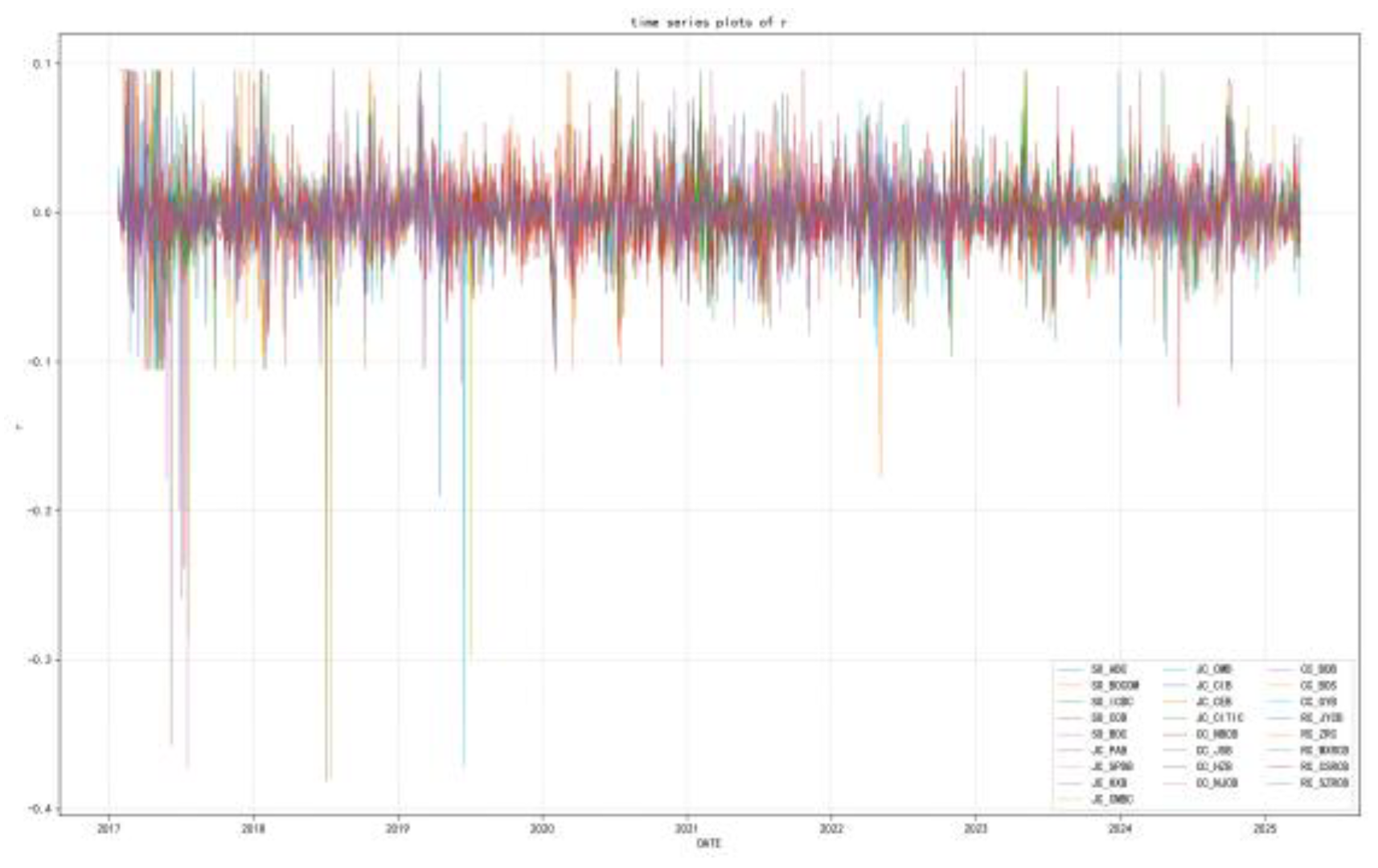
Primarily, the research work calculated the summary statistics for the closing stock market prices of the banks (Table A1). From the empirical research study, it has been identified that the time series processes represent the characteristics of stylized facts of leptokurtosis, fat tails, asymmetry, and non-stationary processes. Additionally, as observed from Figure 1, signifies that all the 25 banks systematically co-move. Specifically, the COVID-19 pandemic between 2020 and 2022, domestic stimulus packages dated September 2024, and US-China tariff tensions that surfaced in early 2025. All these characteristics provide robust empirical evidence of dynamic interdependence.
To transform the daily closing prices into a stationary series and resolve problems caused by data scaling and heteroscedasticity, the following equation is used for calculating logarithmic returns:
where Pit denotes the daily closing stock price of bank i at time t.
Table 3 below shows the descriptive statistics and the unit root tests for the logarithmic returns on the 25 sampled banks.
As seen in Table 3, while the volatility is low in the majority of banks, there exist some volatility levels in the RCBs and CCBs. Concerning the distributional morphology, all the series depict the existence of skewness and leptokurtosis. Furthermore, the mean of all the series tends towards zero, the existence of neither trend nor seasonal factors, as is evidenced by the Figure A1. In addition, the P-values of the ADF test reject the hypothesis of the existence of a unit root, hence, all the series can be validated as stationary time series, making the subsequent empirical modeling feasible.
3.2. Dynamic Evolution of Interbank Risk Transmission and Systemic Importance Analysis
The COVID-19 pandemic is used as the key exogenous shock in this analysis. This section systematically investigates interbank risk spillovers over three different periods, and also investigates the complicated process of systemic risk transmissions in the banking industry.
3.2.1. Analysis of Aggregate and Localized Spillovers
The process starts by analyzing the total spillover index at the aggregate level. As is shown in Figure 2.
Figure 2 shows that, until 2018, the total risk spillover in the banking industry kept relatively small compared to the latter stages, albeit in a state of extreme volatility. Nevertheless, the post-2018 era experienced a drastic change. Because of the economic slowdown, further financial deleveraging, as well as US-China trade tensions, the channels of risk spillover in the banking industry broadened. As such, the spillover index increased and stayed at a high level. In the year 2020, the coronavirus pandemic brought in the overall macroeconomic shock, which led to stagnation in the majority of industries and disruptions in corporate funds. Because of this, the total spillover index oscillated at a high level, at approximately 95. During the post-pandemic period, industries experienced initial hindrances like labor shortages and supply chain disruptions. When further bolstered by the geopolitical conflicts in 2023, as well as higher volatility in the RMB exchange rate, the risk spillover index increased again to break the 95 threshold after a short-term drop. Later on, as a result of policy optimization and enhanced mechanisms in risk buffering, the spillover index dropped rapidly to the 94 level. Nevertheless, it still stays much higher than the original level in the pre-2018 era.
Based on the classification in Table 1, the dynamics of total spillovers (TO) and total spill-ins (FROM) of each type of bank over periods are examined. As is shown in Figure 3.
Figure 3 reveals the significant heterogeneity of risk spillover for different banking categories in the pre-pandemic, pandemic, and post-pandemic periods. For SOCBs, the total spillover remained at a relatively high level of around 80 before the pandemic, but reduced during the pandemic period, though rebounding in the post-pandemic period after a slump in mid-2023, failing to regain the pre-pandemic level. For JSCBs, there was a positive trend before the pandemic. During the pandemic, the level of spillovers fluctuated in theshort term but remained at a very high level, averaging around 87, thus making JSCBs the major spillover contributor out of the four banking types. This level of spillovers in the post-pandemic period was quick to recover and even surpassed the pre-pandemic level. For CCBs, there was volatility before the pandemic. Before August of 2018, spillovers remained below 65, but afterwards, due to joint effects of economic transformation and financial deleveraging, the spillover index exceeded 80. For the pandemic period, there was a specific drop relative to late 2019. In the post-pandemic period, the recovery of the spillover level was slow but accompanied by large fluctuations. For RCBs, there was a low level of spillovers and a downward trend before the pandemic. A specific drop relative to late-2019 occurred in the pandemic period, and in the post-pandemic period, the total level of spillover was at a relatively low baseline.
The observed dynamical changes are closely linked with bank-specific factors, such as bank-specific characteristics, systemic significance, customer bases and resistance to external shocks. In this respect, SOCBs and JSCBs with high asset levels and complex business networks have a higher degree of risk spillovers. These banks have a relatively fast restoration pattern in the period following the pandemic. In contrast, CCBs and RCBs face restrictions in terms of regional agglomeration, homogeneous business activities and reduced capacities to absorb risk. This causes these banks to have a lower degree in overall risk spillovers and a relatively slower restoration process in the post-pandemic period.
Figure 4 graphs the total spill-in indices (FROM) for the different categories of banks.
As illustrated in Figure 4, the post-2018 period is marked by the overall rise in incoming spillovers (FROM) in the banking industry. Of the various groups, the one that displays largest amounts of volatility is that of SOCBs and JSCBs. The increased sensitivity of SOCBs to external risk transmission is backed by their recognition as Systematically Important Banks, as well as their dense interbank connections. On the same note, the steady push for upward risk exposure for JSCBs is also reflected in the structural hindrances that impede any increase in their interbank transactions, thereby accelerating the spillage of capital and escalating risks associated with operational failures. However, the sensitivity of CCBs and RCBs to risks is only mildly impacted in the pre-pandemic period, primarily because of their specific customer bases. In the wake of the COVID-19 pandemic, the extreme shock in the offline economy triggered the first jump in spill-ins, followed by a sharp withdrawal. At the meantime, the expansion of online activity enabled a swift return in risk interconnectedness. During this turbulent process, overall spillover intensity stayed at higher levels. It should be noted that CCBs showed a dramatic decline in inward spillovers in the course of the COVID-19 pandemic. This is related to the deterioration in the creditworthiness of their major customers, small to medium-sized enterprises, as well as the service sectors, which suffered from the COVID-19 outbreak in an aggravated manner. As such, the strategy of deliberate shrinkage in lending risk as well as the enhancement of risk management rules contributed to a sharp decrease in high-risk trades within the banking system as well as in inward risk spillovers. In the post-pandemic period, there is a swift return in inward risk spillovers in the broader group.
3.2.2. Analysis of Interbank Spillover Intensity and Directionality
In this section, the magnitude and nature of risk transmission for various banking groups are examined. Two approaches are used for analysis, namely Net Spillovers (NET) and Pairwise Net Spillovers (Pairwise-NET). These are represented through Figure 5 and Figure 6, respectively.
Figure 5 illustrates the paths of the net spillovers during the pre-pandemic, pandemic, and post-pandemic periods. In the pre-pandemic period, the SOCBs, JSCBs and RCBs were found to principally have a net spillover of negative values, which indicated the role of these banks as the net risk recipients, while the CCBs displayed positive values and were identified as the primary net risk transmitters during this period. Following the outbreak, SOCBs took on critically important policy roles and absorbed systemic risks posed by other banks. Following 2020, the net risk outflow exhibited fluctuations between positive and negative values, with the overall trend being predominantly negative. Consequently, as the pandemic persisted, SOCBs strengthened their risk resilience. Coupled with government policy support, they effectively countered the pandemic’s economic impact, gradually becoming net risk transmitters. In contrast, CCBs demonstrated an alternate trend. They initially had a positive net spillovers. However, they transitioned to negative after 2021. JSCBs, on the other hand, experienced a considerable reduction in net spillovers after 2020. They generally ended up low levels between 2020 and 2021 and even turned negative. However, due to increased economic turmoil and pandemic spread, they eventually became the principal net risk transmitters during this period. Concurrently, RCBs experienced a slight increase in net values after 2020. However, they remained negative and continued to be net risk recipients.After the pandemic, the risk transmission function for SOCBs normalized slowly and reached the level where they were net risk recipients. Conversely,the continuous business expansion of JSCBs has resulted in their repositioning as the primary net risk transmitters. The continuous business expansion of JSCBs has resulted in their repositioning as the primary net risk transmitters. At the same time, CCBs increased their interbank interactions, leading to an overall change in their spillovers from negative to positive. Moreover, due to rural revitalization policies and increased interbank collaborations, RCBs enhanced their capabilities for risk transmission. This caused these banks to take up their role as net risk transmitters after 2024.
Figure 6 shows the pairwise risk transmission pathwaysand the evolution of their intensity and directionality across different periods. At the start, the intensity of risk transmission between SOCBs and the remaining three categories of banks was considerable. Before the pandemic, SOCBs primarily functioned as the net risk recipients, with JSCBs exhibiting a stronger intensity of risk spillover to SOCBs. During the pandemic, the net spillovers of SOCBs revealed a pattern of alternations between positive and negative spillovers. After the pandemic, the ability of SOCBs to transmit risks was restored, and SOCBs ultimately became the net risk recipients once again. Second, the study examines the effect of JSCBs on CCBs and RCBs. Prior to the pandemic, JSCBs were the primary net receivers of risks emanating from CCBs. However, the spillover effect of JSCBs on RCBs was insignificant, their spillover effects on RCBs fluctuated around zero.After the pandemic, the net risk spill-over effect from JSCBs to CCBs strengthened progressively after 2020. In 2021, this effect went from negative to positive, making JSCBs net risk transmitters to CCBs. At the same time, JSCBs remained largely net risk transmitters to RCBs. In the post-pandemic period, through the accelerated growth of businesses of JSCBs, they remained entrenched as net risk transmitters to both CCBs and RCBs, accompanied by strengthened capabilities of output. Lastly, on the relationship between CCBs and RCBs, there seems to be an overall stability in that CCBs have consistently acted as net risk transmitters in all periods.
3.2.3. Robustness Checks
To verify how robust the empirical findings are, robustness tests are performed on the model parameters. Two methods are used. First, the lag order is modified from 3 to 1 and 2. Second, the value of the forgetting factor is changed from 0.99 to 0.95. The new dynamic total spillover indices derived using the different model parameters are given in Figure 7.
Figure 7 illustrates that the variation in the lag orders and the values of the forgetting factors produces only marginal differences in the magnitude of the total spillover indices. Even though there exist some marginal differences, the indexes still remain relatively highly comparable. Furthermore, The more important aspect is the similarity in the pattern over time for all specifications. This consistency substantiates the robustness and validity of the empirical model.
3.3. Analysis of Systemic Importance
3.3.1. Analysis of Systemic Importance across Banking Categories
For the purpose of gaining an intuitive understanding of systemic importance in the banking industry, network topology is used to identify the structural characteristics of the risk network. Figure 8 illustrates the changes of systemic importance in the pre-pandemic, pandemic, and post-pandemic period. For these network graphics, nodes are used to represent particular banking categories. For the nodes, the size of each node is determined by its weighted out-degree centrality, and the largest nodes indicate institutions acting as the primary sources of risk spillovers for the particular period. On the connecting edges, they denote the net risk spillovers between banking institutions, and the red edges indicate the net export of risk from node i to node j, and the blue edges indicate the net import of risk by node i from node j. Additionally, the thickness of the edges represents the absolute value of the net risk spillovers, where the thick edges indicate greater risk transmissions.
As demonstrated in Figure 8, there are distinct risk spillover interconnections among banking categories across the three periods. In the pre-pandemic, CCBs were identified as the core risk source. The major transmission paths were shown to be from CCBs to SOCBs and JSCBs. Moreover, the transmission from JSCBs to SOCBs was also observed. During the pandemic, the CCBs maintained a prominent role as a risk factor, followed by JSCBs. Among the network dynamics, there were three major: the bidirectional transmission between CCBs and SOCBs, the one-way transmission from JSCBs to SOCBs, and the different net risk transmissions from RCBs to CCBs, and from CCBs to JSCBs. In the post-pandemic period, the core risk source became the RCBs, followed by JSCBs as a secondary provider. There were two major risk transmission paths: the net risk outflow from RCBs to SOCBs, and from SOCBs to CCBs.
3.3.2. Bank-Level Assessment of Systemic Importance in Different Periods
To better understand the systemic importance, this subsection undertakes an assessment of 25 individual banks. It employs a dynamic risk network approach, examining shifts in core risk sources and risk transmission pathways across different time periods. The full network structure is represented in Figure 9. There is significant diversification in the nature and levels of risk spillovers between the banks in the three periods.
To enhance the identification of key transmission paths and core risk sources, a filtered network topology is also generated (see Figure 10). For this filtered graph, key transmission paths are shown in yellow color, while core risk sources are mapped using orange color. The filter criteria are defined in the following manner: “critical pathways” are defined as the weights in the upper 20%, while the four institutions that have the highest rankings in centrality are identified to be core risk sources.
Figure 10 explains critical transmission paths that provide a more intuitive understanding of change in characteristics and trends in interbank risk transmission. Prior to the pandemic, red lines (net risk outputs) were mainly concentrated around JSCBs, and blue lines (net risk inputs) were mainly concentrated on SOCBs. This showed that interbank risk transmission mainly took place from JSCBs to SOCBs. During the pandemic, the distribution of red edges became markedly dispersed. A significant increase in red edges was observed for RCBs and CCBs. which showed that RCBs and CCBs became major risk transmitters. Specifically, Minsheng Bank showed major transmission outwards. Additionally, there was increased concentration of blue lines in RCBs and CCBs to demonstrate that there was increased risk input by these banks. Notably, both red and blue lines became more uniform to demonstrate decentralization in interbank risk transmission. More importantly, interbank risk transmission during that period was mainly from risk inputs. After the pandemic period, interbank risk transmission showed that both red and blue lines mainly concentrated on JSCBs and SOCBs to demonstrate that they are major transmitters of interbank risks. Additionally, blue lines mainly concentrated on SOCBs again to demonstrate that SOCBs faced major risks from interbank transactions. Interbank risk transmission during that period took mainly risk outflows.
Based on the calculations, Table 4 presents the systemic importance ranking and the key transmission Paths in the top 20% of the weighted edges.
As illustrated in Table 4, the findings demonstrated highlight the clear changes that have occurred in the rankings and transmission channels over the three periods. In the pre-pandemic, it is clear that the core risk sources included CMB, NBCB, PAB and CIB, which comprised mainly JSCBs and CCBs, with high intensity of risk output. The major transmission paths during that period came from both CIB and CMB, and the paths pointed towards the ABC. This indicates that the ABC had a major role as a risk recipient.During the pandemic, JRCB, BOS, CMBC and SZRCB were identified as the primary core risk sources. These banks are constituents of the RCBs and CCBs. This result further reinforces the view of the significantly effect of the systemic shock on the client bases of RCBs and CCBs. It should be noted that JRCB can be viewed as a representative case. The main paths of this period remained centered on the outflows of risks from JRCB to CMB and CIB. In the post-pandemic period, BOC, ABC, BOCOM and CIM have been identified as core risk sources. The major risk transmission channels have been found to be risk outflows from BOC to CMB and risk outflows from BOC to CIB.
4. Discussion and Conclusions
On the basis of the preceding empirical analysis, the key findings are given below:
1) The pandemic had a significant impact on the banking industry. There is evidence to show that total spillover amounts during and after the pandemic were considerably higher than in the pre-pandemic period, which is an indication of an enhanced level of systemic risk following the shock. 2) The banking system is characterized by heterogeneity and time-varying properties. Prior to the pandemic, CBBs and JSCBs served as the major net risk transmitters. CBBs specifically appeared to be the core risk source, with key risk transmission paths extending to SOCBs and JSCBs. After the pandemic, JSCBs and CBBs remained the core risk sources, with key risk transmission paths from JSCBs and CBBs to SOCBs. On the other hand, SOCBs and RCBs appeared to be the major net risk recipients overall. In the paired net spillover analysis, it was once again demonstrated that SOCBs predominantly function as net recipients of risk spillovers from the other three categories of banks. 3) Systematic importance analysis of 25 individual banks shows obvious changes in core risk sources. Before the pandemic, risk concentration was dominated by CMB, NBCB, PAB and CIB. In the pandemic, risk concentration changed to JRCB, BOS, CMBC and SZRCB. After the pandemic, system dominance returned to BOC, ABC, BOCOM and CIB.
On the basis of the empirical evidence, a differential regulatory approach is proposed. For the SOCBs, it is necessary to focus on improving the capacities of risk buffering, accompanied by high capital-adequacy ratio maintenance, which is a prerequisite to counter the inherent risks facing such banks as the principal receivers of risk. With regard to the regulation of the JSCBs and the CCBs, it is necessary to focus on monitoring the risk transmission channels. It is recommended to establish differential liquidity management indicators, along with limited development of high-risk business. For the RCBs, it is necessary to improve the cooperative mechanisms of financial risk defense at the county levels. Moreover, there is a need to strengthen the risk-isolation mechanisms to improve the difference between such banks and other banking sectors. On the other hand, it is necessary to attempt to improve the dual-track approach of regulation, namely the “Risk Source-Transmission Pathway,” to respond to dynamic changes in core risk sources. It is necessary to set inter-institutional limits of exposure to trigger critical transmission channels. Overall, such approaches are believed to be useful in improving the forward-looking functions and efficiency of financial regulation.
Despite the extensive analysis of dynamic risk spillovers, core risk sources, and transmission paths under external shocks, a number of weaknesses still exist. First, financial markets are characterized by natural asymmetry, which has been left unaccounted for in the model selection. Second, heterogeneity at a regional level has not been incorporated into the analysis.
Author Contributions
Conceptualization, X.W. and C.L.; methodology, C.L. and H.M.; validation, X.W., C.L. and S.Z.; formal analysis, H.M. and Z.Q.; data curation, C.L. and Z.Q.; writing—original draft preparation, C.L., X.W. and H.M.; writing—review and editing, C.L., X.W., S.Z. and H.M.; supervision, X.W. and C.L.; funding acquisition, C.L., H.M. and S.Z.. All authors have read and agreed to the published version of the manuscript.
Funding
This research was funded by National Natural Science Foundation of China, grant number 12301632;Natural Science Foundation of Shandong Province, grant number ZR2023QA004; Natural Science Foundation of Shandong Province, grant number ZR2022MG045; Shandong Provincial Key Research Base for Social Science Theory-Shandong Digital Economy Research Base Fund, , grant number SDSZJD202303.
Data Availability Statement
All data have been uploaded to Science DB ( https://doi.org/10.57760/sciencedb.29260). The other original data can be obtained from the authors upon reasonable request.(34049@sdwu.edu.cn).
Conflicts of Interest
The authors declare no conflicts of interest.
Appendix A

Table A1.
Descriptive Statistics and Stationarity Tests of Daily Price.
| Bank name | mean | sd | skew | kurtosis | se | P value | Bank name | mean | sd | skew | kurtosis | se | P value |
|---|---|---|---|---|---|---|---|---|---|---|---|---|---|
| SO_ABC | 3.572 | 0.561 | 1.099 | 0.924 | 0.013 | 0.9092 | CC_NBCB | 26.135 | 7.454 | 0.453 | -0.857 | 0.167 | 0.5518 |
| SO_BOCOM | 5.665 | 0.861 | 0.437 | -0.573 | 0.019 | 0.7163 | CC_JSB | 7.247 | 1.054 | 0.881 | 0.314 | 0.024 | 0.5271 |
| SO_ICBC | 5.284 | 0.648 | 0.641 | 0.223 | 0.015 | 0.7968 | CC_HZB | 12.374 | 3.237 | 0.753 | 1.172 | 0.073 | 0.2818 |
| SO_CCB | 6.707 | 0.785 | 0.742 | 0.589 | 0.018 | 0.7615 | CC_NJCB | 9.022 | 1.27 | 0.315 | -0.792 | 0.028 | 0.4269 |
| SO_BOC | 3.724 | 0.581 | 1.154 | 0.997 | 0.013 | 0.9169 | CC_BOB | 5.569 | 1.312 | 1.52 | 2.114 | 0.029 | 0.03128 |
| JC_PAB | 13.396 | 3.585 | 1.137 | 0.809 | 0.08 | 0.5024 | CC_BOS | 9.997 | 4.754 | 1.694 | 2.222 | 0.107 | 0.02236 |
| JC_SPDB | 9.963 | 2.241 | 0.583 | 0.16 | 0.05 | 0.0957 | CC_GYB | 8.793 | 3.64 | 0.885 | -0.576 | 0.082 | 0.05852 |
| JC_HXB | 7.01 | 1.562 | 0.991 | 0.457 | 0.035 | 0.139 | RC_JRCB | 5.491 | 3.298 | 3.182 | 10.931 | 0.074 | 0.1651 |
| JC_CMBC | 5.318 | 1.69 | 0.735 | -0.63 | 0.038 | 0.02068 | RC_ZRC | 6.696 | 3.925 | 2.988 | 10.408 | 0.088 | 0.2204 |
| JC_CMB | 35.592 | 8.486 | 0.584 | 0.031 | 0.19 | 0.7082 | RC_WXRCB | 6.457 | 2.359 | 3.408 | 14.112 | 0.053 | 0.2257 |
| JC_CIB | 17.79 | 2.146 | 1.061 | 1.37 | 0.048 | 0.6238 | RC_CSRCB | 7.652 | 1.405 | 2.206 | 5.884 | 0.032 | 0.3622 |
| JC_CEB | 3.638 | 0.461 | -0.1 | -1.046 | 0.01 | 0.4767 | RC_SZRCB | 6.238 | 3.04 | 2.707 | 7.184 | 0.068 | 0.0507 |
| JC_CITIC | 5.742 | 0.763 | 0.083 | -0.884 | 0.017 | 0.5202 |
Figure A1.
Logarithmic Return Time Series Plot.
References
- Allen, F.; Gale, D. Financial contagion. J. Polit. Econ. 2000, 108(1), 1–33. [Google Scholar] [CrossRef]
- Fan, Z.; He, P.; Liu, Z. Financial Contagion, Market Freezes, and Prudential Policies in the Interbank Market-A Network Perspective. Journal of Financial Research 2024, 02, 38–56. [Google Scholar]
- Yang, K.; Wang, J.; Tian, F. Bank network structure and systemic financial risk contagion. Systems Engineering-Theory & Practice. 2024, 44(07), 2120–2136. Available online: https://link.cnki.net/urlid/11.2267.N.20240402.1356.006.
- Zhang, X.; Zhou, R.; Li, Y. Research on the Network Connectivity and Risk Contributions of China’s Systemically Important Banks: A Perspective of Extreme Event Shocks. Journal of Central University of Finance & Economics. 2025, 04, 24–40. [Google Scholar] [CrossRef]
- Ma, J.; Pang, X.; Zhu, S. Measurement and evaluation of systemic risk for China’s banking system. Journal of Management Sciences in China. 2023, 26(12), 85–118. [Google Scholar] [CrossRef]
- Liang, Q.; Li, Z.; Hao, X. Identification and Regulation of Systemically Important Financial Institutions in China-An Analysis Based on the Systemic Risk Index SRISK Methodology. Journal of Financial Research 2013, 9, 56–70. [Google Scholar]
- Diehold, F.X.; Yilmaz, K. On the Network Topology of Variance Decompositions: Measuring the Connectedness of Finance Firms. J. Econom 2014, 182(1), 119–134. [Google Scholar] [CrossRef]
- Antonakakis, N.; Chatziantoniou, I.; Gabauer, D. Refined measures of dynamic connectedness based on time-varying parameter vector autoregressions. J. Risk Financ. Manag. 2020, 13, 84. [Google Scholar] [CrossRef]
- Guo, N.; Zhang, J. A Study on Volatility Spillovers between China’s Energy Market and Stock Market-An Empirical Study Based on TVP-VAR-DY Model. Journal of Southwest Minzu University (Humanities and Social Sciences Edition) 2022, 43(05), 122–133. [Google Scholar]
- Cai, H.; Lan, F. Research on China’s High Level Financial Openness from the Perspective of Financial Security. Studies of International Finance 11, 16–27. [CrossRef]
- Wu, T.; Tang, H.; Xu, D. Study on the Path of RMB Internationalization Based on Carbon Trading--Insights from Empirical Evidence in European Carbon Trading Markets. Studies of International Finance 2024, 08, 61–72. [Google Scholar] [CrossRef]
- He, J.; Zhu, L. On the Dynamic Relationship between the Monetary Policy and the Macro Leverage and Financial Stability--Based on the Construction of China’s Financial Stability Index. Jinan Journal(Philosophy & Social Sciences) 2023, 45(12), 110–128. [Google Scholar]
- Dai, Z.; Zhang, X.; Yin, Z. Extreme time-varying spillovers between high carbon emission stocks, green bond and crude oil: Evidence from a quantile-based analysis. Energy Econ. 2023, 118, 106511. [Google Scholar] [CrossRef]
- Demirer, M.; Diebold, F. X.; Liu, L.; et al. Estimating global bank network connectedness. J. Appl. Econom. 33(1), 1–15. [CrossRef]
- Chen, S.; Li, J.; Tan, L.; Yang, H. The High-Dimensional Time-Varying Measurem -ent and Transmission Mechanism of Systemic Financial Risk in China. The Journal of World Economy 2021, 12, 28–54. [Google Scholar] [CrossRef]
- Bai, L.; Wei, Y. Information spillovers between investor’s public health emergency attention and industrial stocks: Empirical evidence from TVP-VAR model. Journal of Management Science 2024, 32(01), 54–64. [Google Scholar] [CrossRef]
- Li, X.; Li, B.; Wei, G.; Bai, L.; Wei, Y.; Liang, C. Return connectedness among commodity and financial assets during the COVID-19 pandemic: Evidence from China and the US. Resour. Policy 2021, 73, 102166. [Google Scholar] [CrossRef]
- Hu, L.; Wang, Z.; Hu, S.; Shi, W.; Wang, S.; Wang, Y. A Study on the Transnational Spillover Effects of Bank Risk and Sovereign Risk–From the Perspective of COVID-19 Epidemic Situation. Front. Public Health 2022, 10, 940126. [Google Scholar] [CrossRef]
- Koop, G.; Korobilis, D. Large Time-Varying Parameter VARs. J. Econom 2013, 177, 185–198. [Google Scholar] [CrossRef]
- Chen, S.; Tan, L.; Yang, H.; Cui, J. A study on the systemic importance of financial industries:A complex network analysis based on HD-TVP-VAR model. Systems Engineering -Theory & Practice 2021, 41(8), 1911–1925. [Google Scholar]
- PersaranH, H.; Shin, Y. Generalized impluse response analysis in linear multivariate moedls. Econ. Lett. 1998, 58(1), 17–29. [Google Scholar] [CrossRef]
- Liu, C.; Ma, H.; Wang, X.; Cui, J.; Shen, X. A comparative study of dynamic risk spillovers among financial sectors in China before and after the epidemic. PLoS One 2024, 19(12), e0314071. Available online: https://journals.plos.org/plosone/article?id=10.1371/journal.pone.0314071. [CrossRef] [PubMed]
Figure 1.
Time series trend charts of 25 banks.
Figure 2.
Dynamic Evolution of the Total Spillover Index. Note: In Figure 2, the area to the left of the red vertical line represents the pre-pandemic period, the area between the red and the blue lines indicates the pandemic period, and the area to the right of the blue vertical line represents the post-pandemic period. This representation has been consistently followed in the analysis that follows.
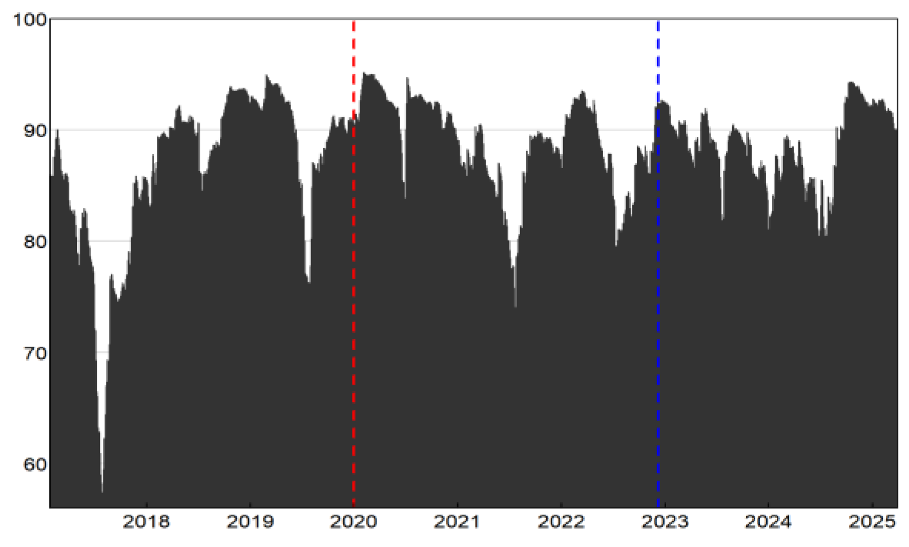
Figure 3.
Dynamic Evolution of TO across Different Banking Categories.
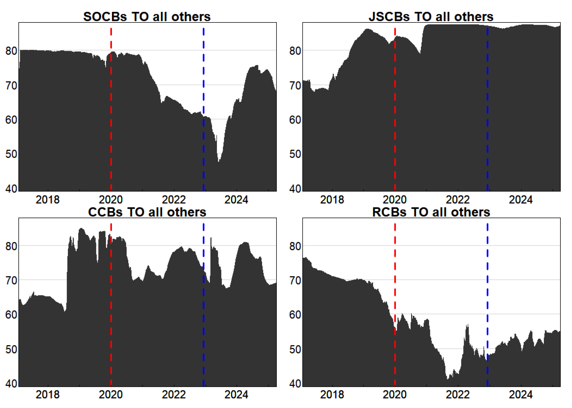
Figure 4.
Dynamic Evolution of FROM across Different Banking Categories.
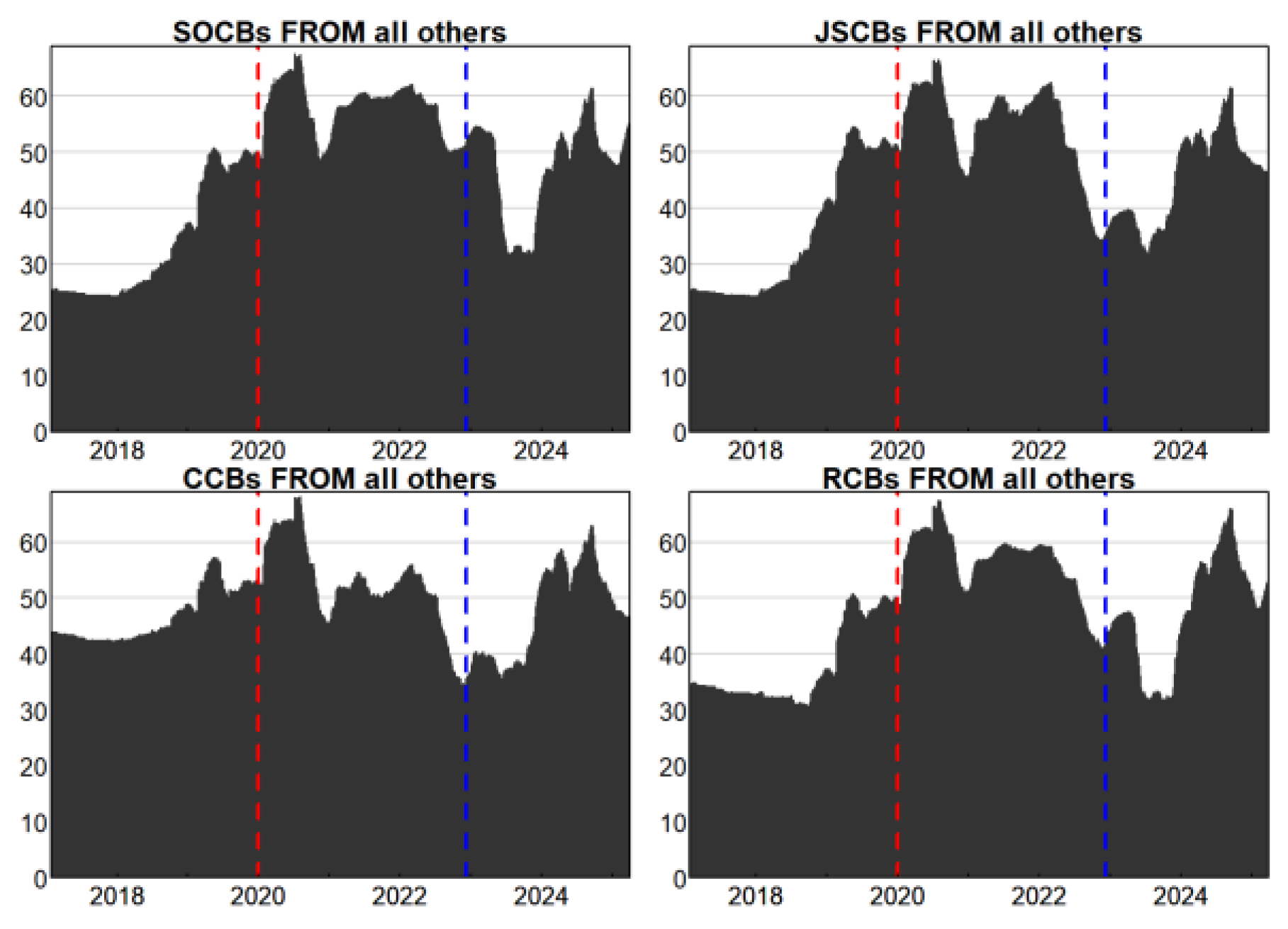
Figure 5.
Dynamic Evolution of Net Spillovers across Different Banking Categories. (left) .
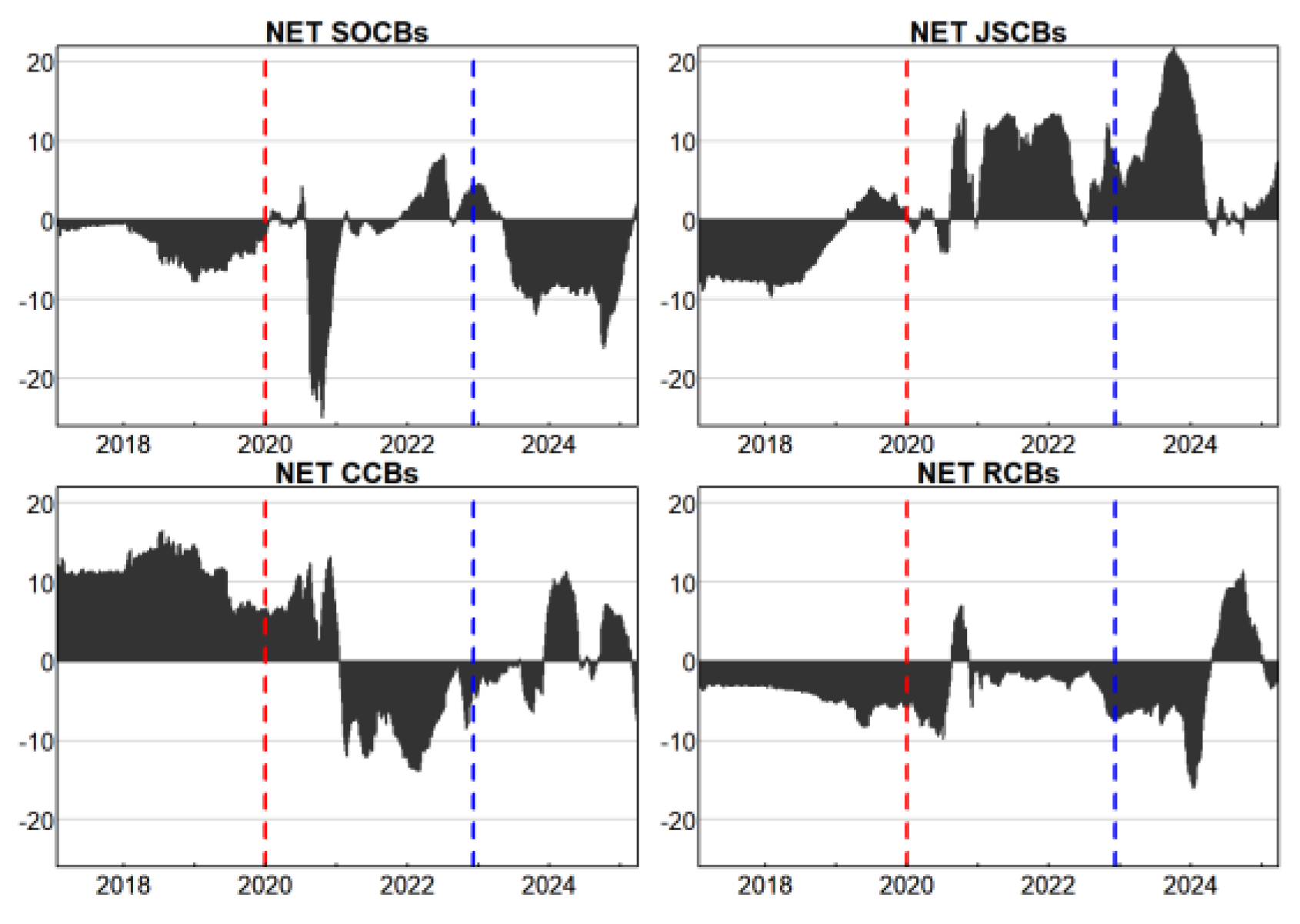
Figure 6.
Dynamic Evolution of Pairwise Net Spillovers between Banking Categories. (right).
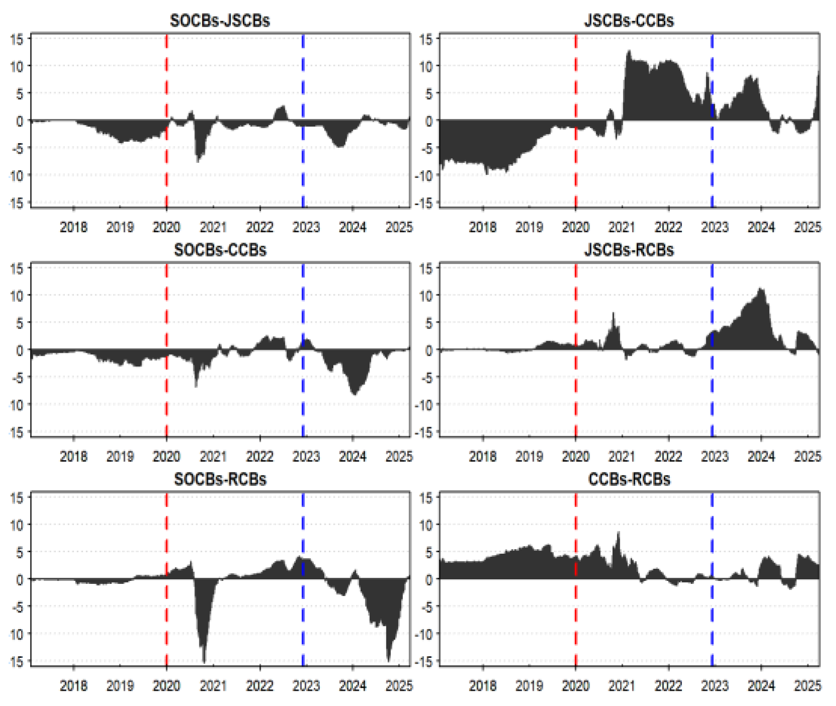
Figure 7.
Comparison of Total Spillover Indices under Alternative Model Specifications.
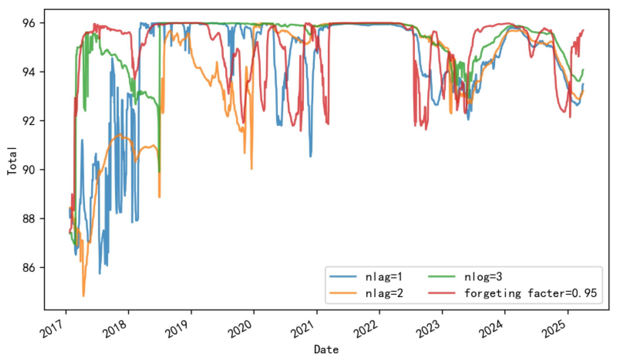
Figure 8.
Risk Network Topologies within the Banking Sector across Different Periods.
Figure 9.
Complex Interbank Risk Network Topology.
Figure 10.
Filtered Interbank Risk Network Topology.
Table 1.
Classification of the Sampled Banking Institutions.
| Banking Classification | Listed Branches Institutions |
Abbreviation | Banking Classification | Listed Branches Institutions |
Abbreviation |
|---|---|---|---|---|---|
| State-owned Banks (Abbreviated as: SOCs) |
Industrial and Commercial Bank of China | ICBC | City Commercial Banks (Abbreviated as: CCBs) | Bank of Beijing | BOB |
| China Construction Bank | CCB | Shanghai Bank | BOS | ||
| Agricultural Bank of China | ABC | Nanjing Bank | NJCB | ||
| Bank of China | BOC | Ningbo Bank | NBCB | ||
| Bank of Communications | BOCOM | Hangzhou Bank | HZBANK | ||
| Joint- stock Commercial Banks (Abbreviated as: JSCBs) |
China Merchants Bank | CMB | Jiangsu Bank | JSB | |
| Industrial Bank | CIB | Guiyang Bank | GYB | ||
| Shanghai Pudong Development Bank | SPDB | Rural Commercial Banks (Abbreviated as: RCBs) | Wuxi Bank | WXRCB | |
| China CITIC Bank | CITIC | Zhangjiagang Bank | ZRC | ||
| Minsheng Bank | CMBC | Changshu Bank | CSRCB | ||
| Everbright Bank | CEB | Suzhou Bank | SZRCB | ||
| Ping An Bank | PAB | Jiangyin Bank | JRCB | ||
| Huaxia Bank | HXB |
Table 2.
Principles for Sample Stage Classification.
| Period | Time Period | Rationale |
|---|---|---|
| pre-pandemic | 2017.1.24- 2019.12.31 |
This period involves significant financial incidents such as the US-Chinese trade dispute of 2018, simultaneous large-scale withdrawals from the P2P lending market, as well as the start of financial deleveraging policies. This stage ends prior to the appearance of the first notifications for COVID-19 cases. |
| during- pandemic | 2020.1.2- 2022.12.8 |
This period consists of two sub-stages: the initial rapid transmission stage (from January 2, 2020, to April 8, 2020), and the normalized prevention and control stage (prior to full reopening) after the Wuhan lockdown lifted (from April 9, 2020, to December 8, 2022). |
| post- pandemic |
2022.12.9- 2025.3.31 |
After December 8, 2022, mandatory nationwide mass PCR screening ceased (excluding Hong Kong, Macao, and Taiwan) to be replaced by voluntary PCR tests (“Yuan Jian Jin Jian”). Thus, the nation shifted to a fully opened normalized stage, which marked the end of the extensive anti-pandemic campaign. |
Table 3.
Descriptive Statistics and Stationarity Tests of Daily Logarithmic Returns.
| Bank name | mean | sd | skew | kurtosis | P- value | Bank name | mean | sd | skew | kurtosis | P- value |
|---|---|---|---|---|---|---|---|---|---|---|---|
| SO_ABC | 0.025 | 1.105 | -0.262 | 7.608 | 0.01 | CC_NBCB | 0.019 | 2.115 | -0.280 | 9.559 | 0.01 |
| SO_BOCOM | 0.011 | 1.124 | -0.631 | 8.915 | 0.01 | CC_JSB | 0.000 | 1.454 | 0.019 | 4.895 | 0.01 |
| SO_ICBC | 0.021 | 1.159 | 0.037 | 5.859 | 0.01 | CC_HZB | -0.016 | 2.114 | -5.038 | 94.335 | 0.01 |
| SO_CCB | 0.023 | 1.333 | -0.075 | 6.086 | 0.01 | CC_NJCB | -0.006 | 1.777 | -4.694 | 99.250 | 0.01 |
| SO_BOC | 0.023 | 1.074 | 0.001 | 10.264 | 0.01 | CC_BOB | -0.026 | 1.175 | -2.971 | 49.633 | 0.01 |
| JC_PAB | 0.010 | 1.954 | 0.312 | 3.063 | 0.01 | CC_BOS | -0.043 | 1.743 | -10.047 | 191.369 | 0.01 |
| JC_SPDB | -0.024 | 1.285 | -1.274 | 22.874 | 0.01 | CC_GYB | -0.049 | 1.621 | -5.789 | 141.958 | 0.01 |
| JC_HXB | -0.019 | 1.255 | -1.924 | 36.772 | 0.01 | RC_JRCB | -0.040 | 2.042 | -0.290 | 11.057 | 0.01 |
| JC_CMBC | -0.044 | 1.192 | -1.996 | 42.483 | 0.01 | RC_ZRC | -0.020 | 2.383 | 0.099 | 7.489 | 0.01 |
| JC_CMB | 0.042 | 1.820 | 0.209 | 2.380 | 0.01 | RC_WXRCB | -0.027 | 2.013 | 0.262 | 6.940 | 0.01 |
| JC_CIB | 0.012 | 1.584 | 0.108 | 4.596 | 0.01 | RC_CSRCB | -0.014 | 2.012 | 0.150 | 5.068 | 0.01 |
| JC_CEB | -0.004 | 1.324 | 0.347 | 6.705 | 0.01 | RC_SZRCB | -0.047 | 2.046 | -1.026 | 17.903 | 0.01 |
| JC_CITIC | 0.001 | 1.517 | 0.279 | 8.057 | 0.01 |
Table 4.
Rankings of Systemic Importance and Key Transmission Pathways. (Top 20% Weighted Edges).
| Period | Rank | Core risk source | Risk output intensity | Rank (Path) | Key Transmission Pathway | Transmission Intensity |
|---|---|---|---|---|---|---|
| Pre-pandemic | 1 | CMB | 40.70124 | 1 | CIB→ABC | 3.294849 |
| 2 | NBCB | 39.93517 | 2 | CMB→ABC | 3.292593 | |
| 3 | PAB | 34.85628 | ||||
| 4 | CIB | 33.24386 | ||||
| during- pandemic | 1 | JRCB | 42.31553 | 1 | JRCB→CMB | 2.335893 |
| 2 | BOS | 33.98259 | 2 | JRCB→CIB | 2.326020 | |
| 3 | CMBC | 18.58274 | ||||
| 4 | SZRCB | 18.57193 | ||||
| post- pandemic |
1 | BOC | 46.10428 | 1 | BOC→CMB | 3.016431 |
| 2 | ABC | 40.39261 | 2 | BOC→CIB | 3.006325 | |
| 3 | BOCOM | 33.76634 | ||||
| 4 | CIB | 24.97696 |
Disclaimer/Publisher’s Note: The statements, opinions and data contained in all publications are solely those of the individual author(s) and contributor(s) and not of MDPI and/or the editor(s). MDPI and/or the editor(s) disclaim responsibility for any injury to people or property resulting from any ideas, methods, instructions or products referred to in the content. |
© 2026 by the authors. Licensee MDPI, Basel, Switzerland. This article is an open access article distributed under the terms and conditions of the Creative Commons Attribution (CC BY) license (http://creativecommons.org/licenses/by/4.0/).
Copyright: This open access article is published under a Creative Commons CC BY 4.0 license, which permit the free download, distribution, and reuse, provided that the author and preprint are cited in any reuse.


