
Submitted:
03 January 2026
Posted:
05 January 2026
You are already at the latest version
Abstract
Based on the derived equation of state for crystals under external stress and temperature, we derived that for non-crystal systems under general external stress and temperature and discussed its relationship with the Macroscopic Mechanical Equilibrium Condition.
Keywords:
equation of state
; external stress
; non-crystals
1. Introduction
The Equation of State (EOS) of a system has a very long history, with the first publication in 1662 [1]. The main purpose of it is to yield the specific fixed volume of a given material under any given external thermal and mechanical conditions. Then, the system must be in a macroscopic equilibrium state.
In fact, the rigorous EOS for any material system can be derived based on the following widely used de facto “theorem" in Statistical Physics, which reflects the first law of thermodynamics. As shown with the Equations (2.95), (3.3), and (3.129) of the statistical thermodynamics book [2] by Bellac, Mortessagne, and Batrouni, the “theorem" may be stated as:
If the infinitesimal work done by the EXTERNAL forces on a system in a macroscopic equilibrium state is written in the form of
where , , …, and are variables independent of each other, then, for any pair of the conjugate variables and , one has
where Z is the partition function of the system, and with Boltzmann constant k and temperature T.
Now let us consider such a system but under isotropic external pressure P. Then the infinitesimal work done by the external force is
where V is the system volume. Then, based on the above “theorem", we have the EOS of the system immediately:
This EOS, applying to any system under external isotropic pressure, is taught in almost any related books [2,3].
2. Crystals Under External Anisotropic Mechanical Conditions
2.1. Crystal Period Vectors and External Stress
A crystal is made of a three-dimensional periodic arrangement of the same cells concisely and tidily. Each cell, containing the same particles, is a parallelepiped. Since a crystal is essentially such an unlimited periodic structure, let us call the edge vectors of the cells as the (crystal) period vectors, shown as red arrows in Figure 1.
The positions of all particles inside the cell, and the crystal period vectors are usually measured through X-ray diffraction experiments. From the pure theory point of view, the particles’ positions can also be calculated by applying the Newtonian Dynamics or Quantum Mechanics. Then what is the theory to calculate the period vectors? Furthermore, crystals may experience rather complicated external mechanical actions. For example, in order to get electric or magnetic field, an additional external pressure is applied onto piezoelectric and piezomagnetic crystals, but only in ONE direction. Here, the external pressures are not the same in all directions. Since the EOS of Eq. (4), for an isotropic pressure, accepting only one pressure value, cannot apply in this situation.
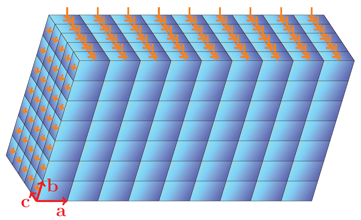
Crystals may also experience external forces containing components parallel to the crystal surfaces, as shown in Figure 2. In general, external forces can be described by the so-called stress. Like pressure (the normal force per unit area), roughly speaking, stress is the total force acting on a surface per unit area “vector". It is expressed as a second-rank tensor ( matrix). The force by the stress acting on the area vector of a surface is .
Still as shown in Figure 2, the crystal period vectors may change independently with each other according to the external stress applied. As the period vectors determine the shape and volume of the cell, then proportional to the macroscopic shape and volume of crystals, the equation determining the period vectors is also the EOS of the crystals. It was derived based on the above “de facto `theorem ’" for general external stress in our recent effort [4,5]. In the following, we will repeat it briefly.
2.2. The Derivation of the EOS
Now let us write the infinitesimal work done by the external stress acting on the surfaces of a crystal cell, which is proportional to that on the surfaces of the whole crystal:
where , , and are surface area vectors.
Then, according to the above “de facto `theorem ’", we have the following equation to determine the period vectors, which is also the EOS for crystals under general external stress and temperature:
2.3. Tuckerman’s Internal Stress
In 2010, Tuckerman introduced the (macroscopic) internal stress of crystals as Equation (5.6.9) in his book [6] (Equation (5.7.9) in the 2023 version):
2.4. Isotropic External Pressure
The isotropic external pressure P is a special case of the external stress . That is , with being the identity tensor. Then, Eq. (6) becomes
which can be further written as
Since the external pressure is the same in all directions, we may assume that the crystal cell expands uniformly when the external pressure changes. This means that all the directions of the period vectors are fixed and their magnitudes are proportional to . In other words, the period vectors depend on the volume only by (implicitly) containing the factor . Once the factor is removed, the period vectors are independent of the volume V:
As a result,
Then using Eq. (13) and Eq. (11),
It reproduces Eq. (4). Therefore, Eq. (6) covers the special case of the isotropic external pressure.
It is better to put Eqs. (14) and (11) together as a summary for the external isotropic pressure condition:
In fact, all these four equations must be satisfied at the same time, and they are satisfied as long as any one of them is satisfied and the crystal expands uniformly with the external isotropic pressure P.
3. Non-Crystal System Under General External Stress
3.1. The EOS
Assuming that the basic physical properties of a non-crystal system do not depend on its macroscopic shape, the system may be regarded as only one but huge crystal “cell" without periodicity in structures, and the “period vectors" are now only the edge vectors of the “cell", but we may still call them the period vectors.
3.2. The Detailed MMEC in Classical Physics
In classical physics, the partition function can be factorized as:
where and are contributed by the kinetic energy and the potential energy of the system, respectively. As in Equations (3.45)–(3.47) in the statistical reference book [2], they can be further expressed as:
where h is the Planck constant and N is the total number of particles in the system. The integration is over all particle momenta in Eq. (17), and over all particle positions within the system volume for Eq. (18).
Then, Eq. (6) becomes
3.2.1. The Thermal Pressure
Since the integration in Eq. (17) has nothing to do with the period vectors, the first term on the right side of Eq. (19), the derivative of the partition function contributed by the kinetic energy, can be written as:
This is the thermal pressure on the cell surfaces, reflecting the forces in the particle collisions and/or the “force associated with the transport of momentum" introduced in our earlier work [7].
3.2.2. The Derivative of Potential Contribution with Respect to the Period Vectors
Now, let us take the derivative of the partition function contributed by the potential energy, the second term on the right side of Eq. (19), by using of Eq. (18):
Here, the derivative is with respect to the period vectors, which determine the volume V of the “cell", also the region of the integrals in Eq. (18). A careful inspection shows that Eq. (18) is the average of the function , which depends on the particle positions , evenly and fully sampled over the “cell" space Vs. Then, as long as the points are sampled exactly the same way, the calculated average is the same, even if the integrals are changed in some form. In any case, we will try to derive rigorously.
Now let us expand the position vector of each particle in the “cell", with respect to the period vectors as:
where the scaled coordinates , in the range of , can be calculated as
For simplicity, let us consider a general position vector in the “cell", also expanded as where with or . Imagine to evenly cut the “cell" into n blocks along period vector , m blocks along , and l blocks along . By the integral definition, for any function , we have
where is the volume of the tiny intersection of the i-th block along , j-th block along , and k-th block along , and is the center position of the intersection. In fact, under the limit of and l all approaching infinity, is the term of the integral of the left side expression of the above equation in mathematics. Meanwhile, the expression in the above equation is the term in the three nested integrals all from 0 to 1 in the next equation, so we have it based on the above equation and the integral definition as:
Please note that the remains the same here as a function of . However, the position is not an independent variable now, but a further function of , as .
Since Eq. (25) applies to every particles, employing Eq. (22) to map every scaled coordinates to the actual particle positions in the system potential energy , the samplings and the average of keep unchanged, if Eq. (18) is rewritten as:
Since the integrals are of fixed regions now, the derivative can go inside
Here the particle positions are not independent variables, but expressed as in Eq. (22). In a Cartesian coordinate system, the components of the period vector may be denoted as . Employing Eq. (22), one has
and, for any d-direction,
Let us denote the net force acting on particle i by all other particles as :
with components form of , and use Eqs. (23), (28 - 30) to get:
3.2.3. The Pair-Interaction Contributions
If only consider internal pair-interactions, Eq. (31) can be rewritten as:
where is the force acting on particle i by particle j. Since , we have
Let us consider all geometric planes cutting through the “cell" but parallel to . The total number (amount) of the planes may be defined as , as it is proportional to the length of the period vector . Then, between particles j and i, there are amount of such planes. Thus, the term in the above equation
means the force between the particles i and j and penetrating and only penetrating the planes between them is averaged across all these planes. Please note that the force is in the direction of , but may be not in the period vector direction.
3.2.4. The Many-Body Interaction Contributions
In actual calculations, three-, four-, and/or even more-body interactions [8,9,10] may also be employed, as in molecular dynamics simulations. By definition, these interactions mean that any of the forces depend on the positions of all the participating particles, then can not essentially be replaced with some pair-interactions in general. Newton’s Third Law may be interpreted as: within a given system, any part may exert force(s) on any other part(s), but cannot accelerate the system itself as a whole, then the net of all forces and the net of all torques within any group of participating particles must be zero. For example, for an M-body interaction (), we have
where is the M-body force on particle k by the rest particles.
If an internal M-body interaction is employed, all the corresponding M-body potentials of various groups of M particles may be included in the system potential of Eq. (18). Then all the forces of each group additionally contribute to Eq. (32), in the form of
where Eq. (36) was employed.
Compared with Eq. (34), Eq. (37) may mean an M-body interaction can be instantaneously regarded as pair-interactions here. In each of the pairs, the net of the two forces is zero. However, they may not point to each other. Although they may generate torque, the total torque of the M-body interaction is zero, as required by the Newton’s Third Law. Then, the M-body interactions contribute the forces over the previously mentioned geometric planes the same way as pair-interactions do.
3.2.5. Conclusions
According to Eqs. (20, 32, 34, 35, and 37 ), the right side of Eq. (19) is the averaged internal forces over all geometric planes cutting the system but parallel to the system surface and over all possible particle position distributions, while the left side is the external force on the surface , then Eq. (19) means the MMEC.
4. Summary
As the EOS, Eq. (6) applies to both crystals and non-crystal systems, under isotropic external pressure or anisotropic external stress and any temperature. It is also the Macroscopic Mechanical Equilibrium Condition of the system.
Acknowledgments
The author wishes to thank Prof. ShiShu Wu, School of Physics, Jilin Univerisity, Changchun, China, Prof. ShiWei Huang, Engineering Technologies Department, John Abbott College, Montreal, Mr. QingLu Guan, Ontario Public Service, Toronto, Mr. LiBin Chen, Independent Researcher, Toronto, Mr. ChangAn Sun, Retired Professional Engineer, Toronto, Mr. ZhenYuan Xie, Independent Researcher, Montreal, Canada, for their encouragement and helpful discussion.
References
- https://en.wikipedia.org/wiki/Boyle%27s_law.
- M.L. Bellac, F. Mortessagne, G.G. Batrouni, Equilibrium and Non-equilibrium Statistical Thermodynamics (Cambridge University Press, Cambridge, 2004).
- O.L. Anderson, Equations of State of Solids for Geophysics and Ceramic Science (Oxford University Press, Oxford, 1995).
- Liu, G. A new equation for period vectors of crystals under external stress and temperature in statistical physics: mechanical equilibrium condition and equation of state. Eur. Phys. J. Plus 136, 48 (2021). [CrossRef]
- Liu, G. Crystal Period Vectors under External Stress in Statistical Physics. Preprints 2019, 2019040076. [CrossRef]
- M.E. Tuckerman, Statistical Mechanics: Theory and Molecular Simulation (Oxford University Press, Oxford, 2010).
- G. Liu, Can. J. Phys., 93, 974-978 (2015),arXiv:cond-mat/0209372 (version 16).
- G. Liu, Preprints.org 2017, 2017090030. [CrossRef]
- G. Liu, E.G. Wang, D.S. Wang, Chin. Phys. Lett. (1997). [CrossRef]
- G. Liu, E.G. Wang, Solid State Commun. (1998). [CrossRef]
Figure 1.
A crystal is made of the same cells tidily, concisely, and infinitely. The red cell edge vectors are also the period vectors of its periodic structure.
Figure 1.
A crystal is made of the same cells tidily, concisely, and infinitely. The red cell edge vectors are also the period vectors of its periodic structure.
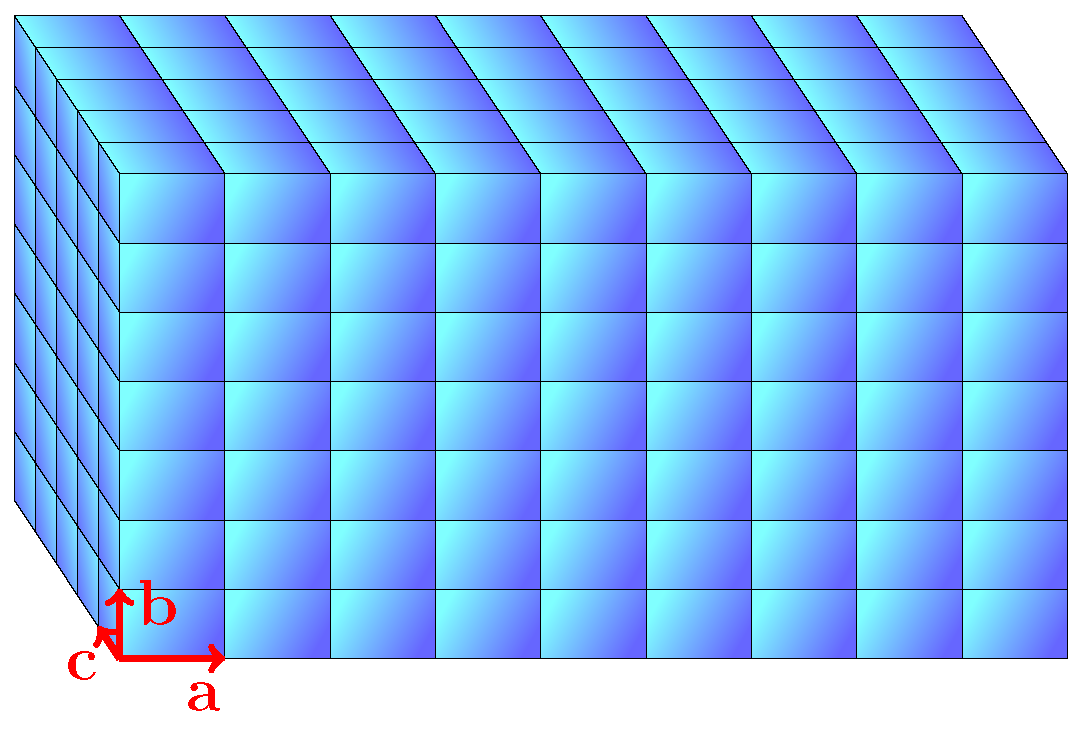
Figure 2.
The crystal and its cells in the previous figure deform when external forces with components parallel to its surfaces are applied on it (the red arrows, other than the period vectors). The period vectors , describing the shapes and volumes of the cells, are also changed.
Figure 2.
The crystal and its cells in the previous figure deform when external forces with components parallel to its surfaces are applied on it (the red arrows, other than the period vectors). The period vectors , describing the shapes and volumes of the cells, are also changed.
Disclaimer/Publisher’s Note: The statements, opinions and data contained in all publications are solely those of the individual author(s) and contributor(s) and not of MDPI and/or the editor(s). MDPI and/or the editor(s) disclaim responsibility for any injury to people or property resulting from any ideas, methods, instructions or products referred to in the content. |
© 2026 by the authors. Licensee MDPI, Basel, Switzerland. This article is an open access article distributed under the terms and conditions of the Creative Commons Attribution (CC BY) license (http://creativecommons.org/licenses/by/4.0/).
Copyright: This open access article is published under a Creative Commons CC BY 4.0 license, which permit the free download, distribution, and reuse, provided that the author and preprint are cited in any reuse.


